Construction of Directed Assortative Configuration Graphs

Abstract

Constructions of directed configuration graphs based on a given bi-degree distribution were introduced in random graph theory some years ago. These constructions lead to graphs where the degrees of two nodes belonging to the same edge are independent. However, it is observed that many real-life networks are assortative, meaning that edges tend to connect low degree nodes with high degree nodes, or variations thereof. In this article we provide an explicit algorithm to construct directed assortative configuration graphs based on a given bi-degree distribution and an arbitrary pre-specified assortativity.

1 Introduction

Random graphs are used to model large networks that consist of particles, called nodes, which are possibly linked to each other by edges. The study of random graphs goes back to the works of [9] and [10]. Since then, numerous random graph models have been introduced and studied in the literature. For an overview we refer the reader to [5, 8, 21, 20]. Empirical studies of large data sets of real-life networks have shown that in many cases the degrees of two nodes belonging to the same edge are not independent (where the degree of a node is defined to be the number of edges attached to it). It is observed that in some types of real-life networks the degree of a node is positively related to the degrees of its linked neighbors, while in other situations the degree of a node is negatively related to the degrees of its linked neighbors. This property is called assortativity or assortative mixing. It has been discovered by [2, 7, 18] that financial networks typically show negative assortativity and that the strength of the assortativity influences the vulnerability of the financial network to shocks, see also [12]. In contrast, social networks tend to be positive assortative, see for instance [17]. More examples of assortative networks are presented in [16] and [14], where also quantities to measure the assortativity in networks are proposed. On the other hand, there is only little literature on explicit constructions of random graphs showing assortative mixing. For example, [19] and [1] study the construction of graphs based on a given graphical degree sequence, and [3] analyzes assortativity in random intersection graphs.

However, established constructions of directed random graphs based on a given bi-degree distribution, called configuration graphs, lead to non-assortative graphs, see for instance the construction presented in [6]. Here, the bi-degree of a node $v$ is a tuple $(j_{v},k_{v})$, where $j_{v}$ is the number of edges arriving at node $v$ (called in-degree) and $k_{v}$ is the number of edges leaving from node $v$ (called out-degree), and we say that node $v$ is of type $(j_{v},k_{v})$, see Figure 1 for an illustration.

Figure 1: Node $v$ is of type $(1,2)$ and node $w$ is of type $(3,4)$. Edge $e=\langle v,w\rangle$ is of type $(2,3)$.

In this article we extend the non-assortative construction presented in [6] by giving an explicit algorithm which allows to construct directed configuration graphs with a pre-specified assortativity based on a concept introduced in [13]. Namely, [13] proposed to specify the graph not only through their node-types, but also through their edge-types. We define the type of an edge $e=\langle v,w\rangle$ connecting node $v$ to node $w$ by a tuple $(k_{e},j_{e})$ with $k_{e}$ denoting the out-degree of node $v$ and $j_{e}$ denoting the in-degree of node $w$, see Figure 1 for an illustration. This notion of edge-types is directly related to the notion of assortativity. In the positive assortative case $k_{e}$ is positively related to $j_{e}$ meaning that edges tend to connect nodes having similar degrees, and accordingly for the negative assortative case. If $k_{e}$ is independent of $j_{e}$, then the graph is non-assortative. This motivated [13] to construct directed assortative configuration graphs based on a given node-type distribution $P$ describing the nodes and from a given edge-type distribution $Q$ describing the edges, while different choices of $Q$ result in different types of assortativity in the constructed graphs, see Figure 2 for examples.

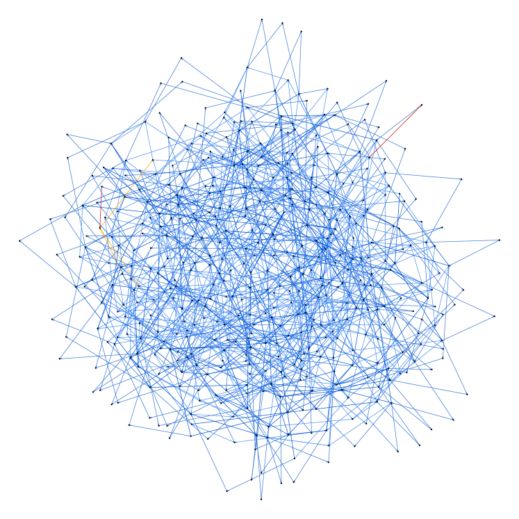
(a) negative assortativity

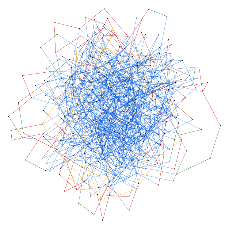
(b) non-assortativity

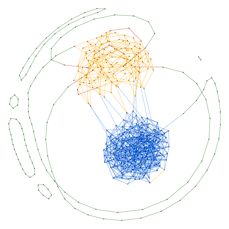
(c) positive assortativity

Figure 2: Three graphs generated by our algorithm given in Section 3 with $N=500$ nodes. They all have the same node-type distribution $P$ but different edge-type distributions $Q$. There are three different types of nodes present in each graph: $(1,1)$, $(2,2)$ and $(3,3)$. Edges of identical type are colored the same. Edges that are arriving or leaving a highest-degree node are colored in different shades of blue. These edges are mainly present in the negative assortative case (a). In the positive assortative case (c), mainly nodes of the same type are connected. These edges are colored dark blue, orange and green. All other possible edges are colored red, which significantly appear only in (b).

Nevertheless, there was not an explicit construction given in [13]. The aim of this article is to construct random graphs where nodes and edges follow pre-specified given bivariate distributions $P$ and $Q$, and we give a precise mathematical meaning to the choice of these distributions.

Let us first interpret the meaning of the distributions $P$ and $Q$ in more detail. Node-type distribution $P$ has the following interpretation. Assume we have a large directed network and we choose at random a node $v$ of that network, then the type $(j_{v},k_{v})$ of $v$ has distribution $P$. Similarly, edge-type distribution $Q$ should be understood as follows. If we choose at random an edge $e$ of a large network, then its type $(k_{e},j_{e})$ has distribution $Q$. This concept of $P$ and $Q$ distributions seems straightforward, however, it needs quite some care in order to give a rigorous mathematical meaning to these distributions, the difficulty lying in the “randomly” chosen node and edge obeying $P$ and $Q$, respectively: the graph as total induces dependencies between nodes and edges which implies that the exact distributions can only be obtained in an asymptotic sense (this will be seen in the construction below).

We give an explicit algorithm to construct a directed assortative configuration graph with a given number of nodes and based on distributions $P$ and $Q$, and we prove that the type of a randomly chosen node of the resulting graph converges in distribution to $P$ as the size of the graph tends to infinity. Similarly, the type of a randomly chosen edge converges in distribution to $Q$. These convergence results give a rigorous mathematical meaning to $P$ and $Q$ in line with their interpretation given above. The proposed algorithm allows for self-loops and multiple edges. In order to obtain a simple graph we delete all self-loops and multiple edges, and we show that the convergence results still hold true for the resulting simple graph. Recently, an alternative approach to construct assortative configuration graphs based on given distributions $P$ and $Q$ was proposed in [11], see also [12], using techniques from [24]. Our construction is different from [11] and more in the spirit of [4, 22, 6]. Moreover, we give a rigorous mathematical meaning to the given distributions $P$ and $Q$ which relies on the law of large numbers only.

In Section 2 we introduce the model and state our main results. Section 3 specifies the algorithm to generate directed assortative configuration graphs. The implementation of the algorithm in the programming language R can be downloaded from:

https://people.math.ethz.ch/~wueth/Papers/AssortativeConfigurationGraphs.R (1.1)

In Section 4 we illustrate examples of assortative configuration graphs generated by our algorithm showing different assortative mixing, and we study their empirical assortativity coefficients as well as their empirical node- and edge-type distributions. The proofs of the results are given in Section 5.

2 Model and main results

Consider fixed finite integers $J\geq 1$ and $K\geq 1$ which describe the maximal in- and out-degree of a node, respectively. For $l\geq 0$ and $n\geq l$ define $[n]_{l}=\{l,\ldots,n\}$. For $j\in[J]_{0}$ and $k\in[K]_{0}$ we say that node $v$ is of type $(j,k)$ if the in-degree of $v$ is $j$ and the out-degree of $v$ is $k$. For $k\in[K]_{1}$ and $j\in[J]_{1}$ we say that a directed edge $e=\langle v,w\rangle$ is of type $(k,j)$ if the out-degree of $v$ is $k$ and the in-degree of $w$ is $j$. Figure 1 illustrates the notions of node- and edge-types. In the remainder, letter $j$ always refers to in-degree and letter $k$ to out-degree. Consider two bivariate probability distributions

$$P = (p_{j,k})_{j\in[J]_{0},k\in[K]_{0}}\qquad\text{with $\sum_{j\in[J]_{0},k\in[K]_{0}}p_{j,k}=1$;}$$

$$Q = (q_{k,j})_{k\in[K]_{1},j\in[J]_{1}}\qquad\text{with $\sum_{k\in[K]_{1},j\in[J]_{1}}q_{k,j}=1$}.$$

We call $P$ node-type distribution and $Q$ edge-type distribution. We denote the marginal distributions of $P$ and $Q$ respectively by

$$p_{j}^{-} = \sum_{k^{\prime}\in[K]_{0}}p_{j,k^{\prime}}\qquad\text{and}\qquad p_{k}^{+}~{}=~{}\sum_{j^{\prime}\in[J]_{0}}p_{j^{\prime},k},\qquad\text{$j\in[J]_{0}$ and $k\in[K]_{0}$; }$$

$$q_{k}^{+} = \sum_{j^{\prime}\in[J]_{1}}q_{k,j^{\prime}}\qquad\text{and}\qquad q_{j}^{-}~{}=~{}\sum_{k^{\prime}\in[K]_{1}}q_{k^{\prime},j},\qquad\text{$k\in[K]_{1}$ and $j\in[J]_{1}$}.$$

In the remainder, superscript “$-$” always refers to in-degree and superscript “$+$” to out-degree. For instance, $(p_{j}^{-})_{j\in[J]_{0}}$ denotes the in-degree distribution of nodes. Observe that in a given graph the number of edges $e=\langle v,w\rangle$ with out-degree of $v$ being $k\in[K]_{1}$ is equal to $k$ times the number of nodes having out-degree $k$, and similarly for the number of nodes having in-degree $j\in[J]_{1}$. This relation between nodes and edges implies that we cannot choose $P$ and $Q$ independently of each other to achieve that nodes and edges in the constructed graph follow $P$ and $Q$, respectively. We therefore assume that $P$ and $Q$ satisfy the following consistency conditions, see also [13] and [11], which implies that the above observation holds true in expectation in graphs where nodes and edges follow distributions $P$ and $Q$, respectively.

$$q_{k}^{+} ~{}=~{}kp_{k}^{+}/z,\qquad k\in[K]_{1};$$ (C1)

$$q_{j}^{-} ~{}=~{}jp_{j}^{-}/z,\qquad j\in[J]_{1},$$ (C2)

with mean degree $z=\sum_{k\in[K]_{0}}kp_{k}^{+}$. Observe that conditions (C1) and (C2) require that $z=\sum_{k\in[K]_{0}}kp_{k}^{+}=\sum_{j\in[J]_{0}}jp_{j}^{-}>0$. This says that, in expectation, the sum of in-degrees equals the sum of out-degrees if nodes and edges follow distributions $P$ and $Q$, respectively.

Remark 2.1.

We assume uniformly bounded degrees. A generalization to unbounded degrees is possible but not straightforward: conditions (C1) and (C2) need to be fulfilled and the rate of decay of $p_{k}^{+}$ and $p_{j}^{-}$ needs a careful specification so that the results below still remain true.

Remark 2.2.

We have defined assortativity through edge-types, which, for an edge $e=\langle v,w\rangle$ connecting node $v$ to node $w$, is defined to be the tuple $(k_{e},j_{e})$ with $k_{e}$ denoting the out-degree of $v$ and $j_{e}$ denoting the in-degree of $w$. There are three other possibilities to define the type of an edge $e$, for instance, by the tuple $(k_{e},k^{\prime}_{e})$ with $k_{e}$ and $k^{\prime}_{e}$ denoting the out-degree of $v$ and $w$, respectively. We comment on these variations of edge-types in more detail in Appendix A.

Given the number of nodes $N\in{\mathbb{N}}$ and given distributions $P$ and $Q$ satisfying (C1) and (C2) the goal is to construct a graph such that the following statement is true in an asymptotic sense as the size $N$ of the graph tends to infinity: the type of a randomly chosen node has distribution $P$ and the type of a randomly chosen edge has distribution $Q$. The following theorem shows that this is indeed the case for graphs constructed by the algorithm provided in Section 3 and, hence, the theorem gives an explicit mathematical meaning to $P$ and $Q$.

Theorem 2.3.

Fix $s\in{\mathbb{N}}$. Let $(j_{v_{1}},k_{v_{1}}),\ldots,(j_{v_{s}},k_{v_{s}})$ be the types of $s$ randomly chosen nodes of the graph generated by the algorithm provided in Section 3. Then,

$$\big{(}(j_{v_{1}},k_{v_{1}}),\ldots,(j_{v_{s}},k_{v_{s}})\big{)}\stackrel{{\scriptstyle d}}{{\longrightarrow}}\big{(}(j^{\prime}_{1},k^{\prime}_{1}),\ldots,(j^{\prime}_{s},k^{\prime}_{s})\big{)},\qquad\text{as $N\to\infty$},$$

where $(j^{\prime}_{1},k^{\prime}_{1}),\ldots,(j^{\prime}_{s},k^{\prime}_{s})$ are $s$ independent random variables having distribution $P$. Similarly, the types of $s$ randomly chosen edges converge in distribution, as $N\to\infty$, to a sequence of $s$ independent random variables having distribution $Q$.

If we consider a graph where nodes and edges follow distributions $P$ and $Q$, respectively, then we expect that the relative number of nodes of type $(j,k)$ is close to $p_{j,k}$ and that the relative number of edges of type $(k,j)$ is close to $q_{k,j}$. Theorem 2.4 below makes this statement precise for graphs constructed by the algorithm provided in Section 3. To formulate the theorem, denote by ${\mathcal{V}}_{j,k}$ the number of nodes of type $(j,k)$, $j\in[J]_{0}$ and $k\in[K]_{0}$, and by ${\mathcal{E}}_{k,j}$ the number of edges of type $(k,j)$, $k\in[K]_{1}$ and $j\in[J]_{1}$, of the constructed graph of size $N$. The total number of edges is denoted by ${\mathcal{E}}$. Theorem 2.4 says that the relative frequencies ${\mathcal{V}}_{j,k}/N$ and ${\mathcal{E}}_{k,j}/{\mathcal{E}}$ converge to $p_{j,k}$ and $q_{k,j}$, respectively, in probability as $N\to\infty$.

Theorem 2.4.

For the random graph constructed by the algorithm provided in Section 3 we have for any $\varepsilon>0$

$$\lim_{N\to\infty}{\mathbb{P}}\left[\sum_{j\in[J]_{0},k\in[K]_{0}}\left|\frac{{\mathcal{V}}_{j,k}}{N}-p_{j,k}\right|+\sum_{k\in[K]_{1},j\in[J]_{1}}\left|\frac{{\mathcal{E}}_{k,j}}{{\mathcal{E}}}-q_{k,j}\right|>\varepsilon\right]~{}=~{}0.$$

The algorithm provided in Section 3 generates a graph possibly not being simple, i.e. it may contain self-loops and multiple edges. To obtain a simple graph we delete (erase) all self-loops and multiple edges, and we call the resulting graph erased configuration graph. The following theorem states that the asymptotic results still hold true for the erased configuration graph.

Theorem 2.5.

The results of Theorem 2.3 and Theorem 2.4 still hold true for the erased configuration graph, based on the algorithm provided in Section 3.

3 Construction of directed assortative configuration graphs

The algorithm to construct directed assortative configuration graphs starts from the work of [6], where the authors construct a directed random graph with $N\in{\mathbb{N}}$ nodes based on given in-degree and given out-degree distributions in the following way. They assign to each node independently an in-degree and an out-degree according to the given distributions, also independently for different nodes. Some degrees are then modified if the sum of in-degrees differs from the sum of out-degrees so that these sums of degrees are equal, and the sample is only accepted if the number of modifications is not too large. Finally, in-degrees are randomly paired with out-degrees. Note that this construction leads to a non-assortative configuration graph and the in- and out-degree of a given node are independent. The construction of an assortative configuration graph is more delicate since in-degrees cannot be randomly paired with out-degrees. In our construction we generate node-types using directly node-type distribution $P$. Independently of the node-types we generate $zN$ edges having independent edge-types according to distribution $Q$. Finally, we match in- and out-degrees of nodes with edges of corresponding types. In general, the matching cannot be done exactly, but with high probability the number of types that need to be changed accordingly is small for large $N$, due to consistency conditions (C1) and (C2). We first describe the algorithm in detail and then comment on each step of the algorithm below.

Algorithm to construct directed assortative configuration graphs.

Assume maximal degrees $J,K\geq 1$ and two probability distributions $P$ and $Q$ satisfying (C1) and (C2) with mean degree $z$ are given. Choose $\delta\in(1/2,1)$ fixed. Choose $N\in{\mathbb{N}}$ so large that there exists $N^{\prime}\in{\mathbb{N}}$ with $N=N^{\prime}+2\left\lceil N^{\delta}\right\rceil+\max\{J^{2},K^{2}\}$, and set $N^{\prime\prime}=N^{\prime}+\left\lceil N^{\delta}\right\rceil$. Here, $\left\lceil x\right\rceil$ denotes the smallest integer larger than or equal to $x\in{\mathbb{R}}$.

1. Step 1. Assign to each node $v=1,\ldots,N^{\prime}$ independently a node-type $(j_{v},k_{v})$ according to distribution $P$. Generate edges $e=1,\ldots,\lceil zN^{\prime\prime}\rceil$ having independent edge-types $(k_{e},j_{e})$ according to distribution $Q$, independently of the node-types. Define

   $$n_{k}^{+} = \sum_{v=1}^{N^{\prime}}1_{\{k_{v}=k\}}\quad\text{ and }\quad e_{k}^{+}~{}=~{}\left\lceil\frac{1}{k}\sum_{e=1}^{\lceil zN^{\prime\prime}\rceil}1_{\{k_{e}=k\}}\right\rceil\quad\text{ for all $k\in[K]_{1}$};$$

   $$n_{j}^{-} = \sum_{v=1}^{N^{\prime}}1_{\{j_{v}=j\}}\quad\text{ and }\quad e_{j}^{-}~{}=~{}\left\lceil\frac{1}{j}\sum_{e=1}^{\lceil zN^{\prime\prime}\rceil}1_{\{j_{e}=j\}}\right\rceil\quad\text{ for all $j\in[J]_{1}$}.$$

   Let $A_{N}$ be the event on which we have

   $$\left|n_{k}^{+}-p_{k}^{+}N^{\prime}\right|\leq p_{k}^{+}N^{\delta}/2 \left|e_{k}^{+}-p_{k}^{+}N^{\prime\prime}\right|\leq p_{k}^{+}N^{\delta}/2\quad\text{ for all $k\in[K]_{1}$};$$ and

   $$\left|n_{j}^{-}-p_{j}^{-}N^{\prime}\right|\leq p_{j}^{-}N^{\delta}/2 \left|e_{j}^{-}-p_{j}^{-}N^{\prime\prime}\right|\leq p_{j}^{-}N^{\delta}/2\quad\text{ for all $j\in[J]_{1}$}.$$ and

   Proceed to Step 2 if event $A_{N}$ occurs. Otherwise, proceed to Step 5.

2. Step 2. For each $k\in[K]_{1}$ and each $j\in[J]_{1}$ do the following.

   • Add $r_{k}^{+}=ke_{k}^{+}-\sum_{e=1}^{\lceil zN^{\prime\prime}\rceil}1_{\{k_{e}=k\}}$ edges of type $(k,1)$;

   • Add $r_{j}^{-}=je_{j}^{-}-\sum_{e=1}^{\lceil zN^{\prime\prime}\rceil}1_{\{j_{e}=j\}}$ edges of type $(1,j)$.

   Set $r^{+}=\sum_{k\in[K]_{1}}r_{k}^{+}$ and $r^{-}=\sum_{j\in[J]_{1}}r_{j}^{-}$.

3. Step 3. Set the type of each node in $\{N^{\prime}+1,\ldots,N\}$ to $(0,0)$. For each $k\in[K]_{1}$ and each $j\in[J]_{1}$ do the following.

   • Take the first $e_{k}^{+}-n_{k}^{+}+r^{-}1_{\{k=1\}}$ nodes in $\{N^{\prime}+1,\ldots,N\}$ having out-degree $0$ and change their out-degrees to $k$;

   • Take the first $e_{j}^{-}-n_{j}^{-}+r^{+}1_{\{j=1\}}$ nodes in $\{N^{\prime}+1,\ldots,N\}$ having in-degree $0$ and change their in-degrees to $j$.

4. Step 4. For each $k\in[K]_{1}$ and each $j\in[J]_{1}$ do the following.

   • Assign to each node having out-degree $k$ exactly $k$ uniformly chosen edges $e$ of type $(k_{e},j_{e})$ with $k_{e}=k$;

   • Assign to every node having in-degree $j$ exactly $j$ uniformly chosen edges $e$ of type $(k_{e},j_{e})$ with $j_{e}=j$.

   Proceed to Step 6.

5. Step 5. Define node-types $(j_{1},k_{1})=(0,1)$, $(j_{2},k_{2})=(1,0)$ and $(j_{v},k_{v})=(0,0)$ for all $v=3,\ldots,N$. Insert an edge $e=\langle 1,2\rangle$ that connects node $1$ to node $2$.

6. Step 6. Return the constructed graph.

Explanation of the algorithm.

We say that node $v$ is a $k$-node if its out-degree is $k\in[K]_{1}$, and similarly we say that edge $e=\langle v,w\rangle$ is a $k$-edge if $v$ is a $k$-node, $k\in[K]_{1}$.

Step 1. We generate only $N^{\prime}$ node-types and we keep $2\lceil N^{\delta}\rceil+\max\{J^{2},K^{2}\}$ nodes undetermined for possible modifications in later steps. The expected number of generated $k$-nodes is $p_{k}^{+}N^{\prime}$ and the expected number of generated $k$-edges is $q_{k}^{+}\lceil zN^{\prime\prime}\rceil$. Using condition (C1), the expected number of $k$-nodes needed for the generated $k$-edges is therefore $q_{k}^{+}\lceil zN^{\prime\prime}\rceil/k\approx p_{k}^{+}N^{\prime\prime}>p_{k}^{+}N^{\prime}$. Henceforth, if $e_{k}^{+}$ is close to its expectation $q_{k}^{+}\lceil zN^{\prime\prime}\rceil/k\approx p_{k}^{+}N^{\prime\prime}$, it dominates the number of generated $k$-nodes $n_{k}^{+}$ which is of order $p_{k}^{+}N^{\prime}<p_{k}^{+}N^{\prime\prime}$. Step 3 is then used to correct for this imbalance in a deterministic way, and event $A_{N}$ guarantees that this correction is possible. For receiving an efficient algorithm we would like event $A_{N}$ to occur sufficiently likely, which is exactly stated in the next lemma.

Lemma 3.1.

We have ${\mathbb{P}}\left[A_{N}\right]\to 1$ as $N\to\infty$.

Integer $N^{\prime\prime}$ is chosen in such a way that, on event $A_{N}$, the number of $k$-nodes needed for the generated $k$-edges dominates the number of generated $k$-nodes, and their difference is at most $2p_{k}^{+}\lceil N^{\delta}\rceil$ for each $k\in[K]_{1}$, see also Figure 3 for an illustration.

Figure 3: On event $A_{N}$, the number of generated $k$-nodes, $n_{k}^{+}$, lies in the interval of length $p_{k}^{+}N^{\delta}$ around $p_{k}^{+}N^{\prime}$. The number of $k$-nodes needed for the generated $k$-edges, $e_{k}^{+}$, lies in the interval of length $p_{k}^{+}N^{\delta}$ around $p_{k}^{+}N^{\prime\prime}$. By definition of $N^{\prime\prime}$ the gap between the two intervals is of size between $0$ and $p_{k}^{+}$. From this it follows that there are at most $2p_{k}^{+}\lceil N^{\delta}\rceil$ additional $k$-nodes needed in order to attach all generated $k$-edges to $k$-nodes.

Therefore, on event $A_{N}$, the total number of additional nodes needed having a positive out-degree is

$$\sum_{k\in[K]_{1}}\left(e_{k}^{+}-n_{k}^{+}\right) \leq 2\lceil N^{\delta}\rceil\sum_{k\in[K]_{1}}p_{k}^{+}~{}\leq~{}2\lceil N^{\delta}\rceil.$$

Hence, we have sufficiently many undetermined nodes in $\{N^{\prime}+1,\ldots,N\}$ to which we can assign out-degrees accordingly in Step 3, and similarly for the in-degrees.

Step 2. In general, the number of generated $k$-edges is not a multiple of $k$. Therefore, we use Step 2 to correct for this cardinality by defining $r_{k}^{+}$ additional edges of type $(k,1)$. Note that each such edge requires a node having in-degree $1$. Therefore, in total $r^{+}\leq K^{2}$ nodes having in-degree $1$ are additionally needed, and similarly for the added edges of type $(1,j)$, $j\in[J]_{1}$. The undetermined $\max\{J^{2},K^{2}\}$ nodes are exactly used to correct for the corresponding node-types in Step 3.

Steps 3 and 4. We assign node-types to the undetermined nodes $N^{\prime}+1,\ldots,N$ in such a way that the total number of $k$-nodes is equal to the number of $k$-nodes needed for the $k$-edges generated in Steps 1 and 2, for each $k\in[K]_{1}$, and similarly for the total number of nodes having in-degree $j\in[J]_{1}$. Then, all cardinalities for $j$ and $k$ match and all edges can be randomly connected to corresponding nodes. After doing so, each node has the correct number of arriving and leaving edges according to its type. Note that this step allows for self-loops and multiple edges.

Step 5. If event $A_{N}$ does not occur in Step 2, we just define a deterministic graph having one edge so that all terms in Theorem 2.3 and Theorem 2.4 are well-defined. Due to Lemma 3.1 the influence of this deterministic graph is negligible.

4 Discussion and examples

Given a non-degenerate node-type distribution $P$ with mean degree $z>0$ given by $z=\sum_{k\in[K]_{0}}kp_{k}^{+}=\sum_{j\in[J]_{0}}jp_{j}^{-}$, we aim to find possible edge-type distributions $Q$ such that $P$ and $Q$ satisfy (C1) and (C2). Conditions (C1) and (C2) imply that the marginal distributions of $Q$ are fully described by the marginal distributions of $P$, and their respective cumulative distribution functions are given by

$$Q^{+}(k)~{}=~{}\sum_{k^{\prime}=1}^{k}q_{k^{\prime}}^{+}~{}=~{}\frac{1}{z}\sum_{k^{\prime}=1}^{k}k^{\prime}p_{k^{\prime}}^{+}\qquad\text{ and }\qquad Q^{-}(j)~{}=~{}\sum_{j^{\prime}=1}^{j}q_{j^{\prime}}^{-}~{}=~{}\frac{1}{z}\sum_{j^{\prime}=1}^{j}j^{\prime}p_{j^{\prime}}^{-},$$

for $k\in[K]_{1}$ and $j\in[J]_{1}$. The possible joint distributions $Q=(q_{k,j})_{k,j}$ are therefore given by

$$q_{k,j} = C\left(Q^{+}(k),Q^{-}(j)\right)+C\left(Q^{+}(k-1),Q^{-}(j-1)\right)$$

$$\hskip 42.67912pt-C\left(Q^{+}(k),Q^{-}(j-1)\right)-C\left(Q^{+}(k-1),Q^{-}(j)\right),$$

where $C:[0,1]^{2}\to[0,1]$ is a $2$-dimensional copula, see for instance [15]. To measure assortativity of a graph, [16] introduced the assortativity coefficient of $Q$ given by

$$\rho_{Q}~{}=~{}\frac{\sum_{k\in[K]_{1}}\sum_{j\in[J]_{1}}kj\left(q_{k,j}-q_{k}^{+}q_{j}^{-}\right)}{\sqrt{\sum_{k\in[K]_{1}}k^{2}q_{k}^{+}-\left(\sum_{k\in[K]_{1}}kq_{k}^{+}\right)^{2}}\sqrt{\sum_{j\in[J]_{1}}j^{2}q_{j}^{-}-\left(\sum_{j\in[J]_{1}}jq_{j}^{-}\right)^{2}}}~{}\in[-1,1],$$

which is Pearson’s correlation coefficient of distribution $Q$, see also [23] for an analysis of different types of correlations in a graph. By Hoeffding’s identity and using representation (4), $\rho_{Q}$ can be rewritten as

$$\rho_{Q}~{}=~{}\frac{\sum_{k\in[K]_{1}}\sum_{j\in[J]_{1}}\big{(}C\left(Q^{+}(k),Q^{-}(j)\right)-Q^{+}(k)Q^{-}(j)\big{)}}{\sqrt{\sum_{k\in[K]_{1}}k^{2}q_{k}^{+}-\left(\sum_{k\in[K]_{1}}kq_{k}^{+}\right)^{2}}\sqrt{\sum_{j\in[J]_{1}}j^{2}q_{j}^{-}-\left(\sum_{j\in[J]_{1}}jq_{j}^{-}\right)^{2}}}.$$

Observe that $\rho_{Q}$ is determined by $P$ and $C$. Define the copulas

$$W(u_{1},u_{2}) = \max\{u_{1}+u_{2}-1,0\};$$

$$M(u_{1},u_{2}) = \min\{u_{1},u_{2}\};$$

$$\Pi(u_{1},u_{2}) = u_{1}u_{2},$$

for $u_{1},u_{2}\in[0,1]$. Then, $C=W$ corresponds to the minimal possible assortativity coefficient $\rho_{Q}^{-}\in[-1,0]$, and $C=M$ corresponds to the maximal possible assortativity coefficient $\rho_{Q}^{+}\in[0,1]$. Copula $C=\Pi$ leads to non-assortativity and in this case we have $q_{k,j}=kjp_{k}^{+}p_{j}^{-}/z^{2}$ for all $k\in[K]_{1}$ and $j\in[J]_{1}$. Note that for given $P$, $\rho_{Q}$ does not uniquely determine $C$. On the other hand, one can always find $\lambda\in[0,1]$ such that $\lambda W+(1-\lambda)M$ leads to a given assortativity coefficient $\rho_{Q}\in[\rho_{Q}^{-},\rho_{Q}^{+}]$. This allows to construct directed assortative configuration graphs having any given assortativity coefficient that is possible for given node-type distribution $P$.

To illustrate assortativity in an example we consider maximal in- and out-degree $J=K=4$ and node-type distribution $P_{p}=\left(p^{p}_{j,k}\right)$, $p\in(0,1)$, given by

$$P_{p}=\begin{pmatrix}0&0&0&0&0\\ 0&0&0&0&0\\ 0&0&p&0&0\\ 0&0&0&0&0\\ 0&0&0&0&1-p\end{pmatrix}.$$

Distribution $P_{p}$ only allows for nodes of types $(2,2)$ and $(4,4)$, with respective probabilities $p$ and $1-p$, which results in a mean degree of $z=4-2p$. Clearly, these nodes can only be connected through edges of types $(2,2)$, $(2,4)$, $(4,2)$ and $(4,4)$. Since $P_{p}$ is diagonal, consistency conditions (C1) and (C2) fully specify the edge-type distribution $Q_{q}$ which is given by

$$Q_{q}=\frac{1}{2-p}\begin{pmatrix}0&0&0&0\\ 0&3p+q-2&0&2-2p-q\\ 0&0&0&0\\ 0&2-2p-q&0&q\end{pmatrix},$$

for $q=q(p)\in[\max\{2-3p,0\},2-2p]$. For fixed $p\in(0,1)$, different values of $q$ lead to different assortativity coefficients $\rho_{q}=\rho_{Q_{q}}$. A straightforward calculation gives

$$\rho_{q}~{}=~{}\frac{q(2-p)-4(1-p)^{2}}{2p(1-p)},\quad\text{ or equivalently }\quad q~{}=~{}\frac{2(1-p)(2+p(\rho_{q}-2))}{2-p}.$$

For any $p\in(0,1)$, the optimal bounds on $\rho_{q}$ are given by

$$-\min\left\{\frac{p}{2(1-p)},\frac{2(1-p)}{p}\right\}~{}=~{}\rho_{p}^{-}~{}\leq~{}\rho_{q}~{}\leq~{}\rho_{p}^{+}~{}=~{}1.$$

Observe that $\rho_{p}^{-}=-1$ if and only if $p=2/3$.

From now on we fix $p=0.5$, meaning that there are nodes of types $(2,2)$ and $(4,4)$ with equal probability. For any $q\in[0.5,1]$ or $\rho_{q}\in[-0.5,1]$, this leads to

$$\rho_{q}~{}=~{}3q-2\in[-0.5,1]\quad\text{ or equivalently }\quad q~{}=~{}\frac{\rho_{q}+2}{3}\in[0.5,1].$$

A value of $q=1$ results in a graph with maximal assortativity coefficient $\rho_{1}=\rho^{+}_{0.5}=1$. In this case, there are only edges that connect nodes having identical types. By decreasing $q$ we allow also for edges of types $(2,4)$ and $(4,2)$, while we reduce the probability of having edges of types $(2,2)$ and $(4,4)$. If we decrease $q$ to its minimal value $q=0.5$, edges of type $(2,2)$ finally disappear and there are only edges of types $(2,4)$, $(4,2)$ and $(4,4)$. This means that if $q=0.5$, each edge is leaving from a node with maximal possible out-degree or is arriving at a node with maximal possible in-degree. In this case, the assortativity coefficient is negative and given by $\rho_{0.5}=\rho_{0.5}^{-}=-0.5$. Non-assortativity is given for $q=2/3$. To illustrate these different types of assortativity, Figure 4 shows six graphs generated by the algorithm given in Section 3 with $N=1000$ nodes, with node-type distribution $P=P_{0.5}$ and edge-type distribution $Q_{q}$ for values of $q$ such that $\rho_{q}\in\{-0.5,0,0.4,0.6,0.8,1\}$.

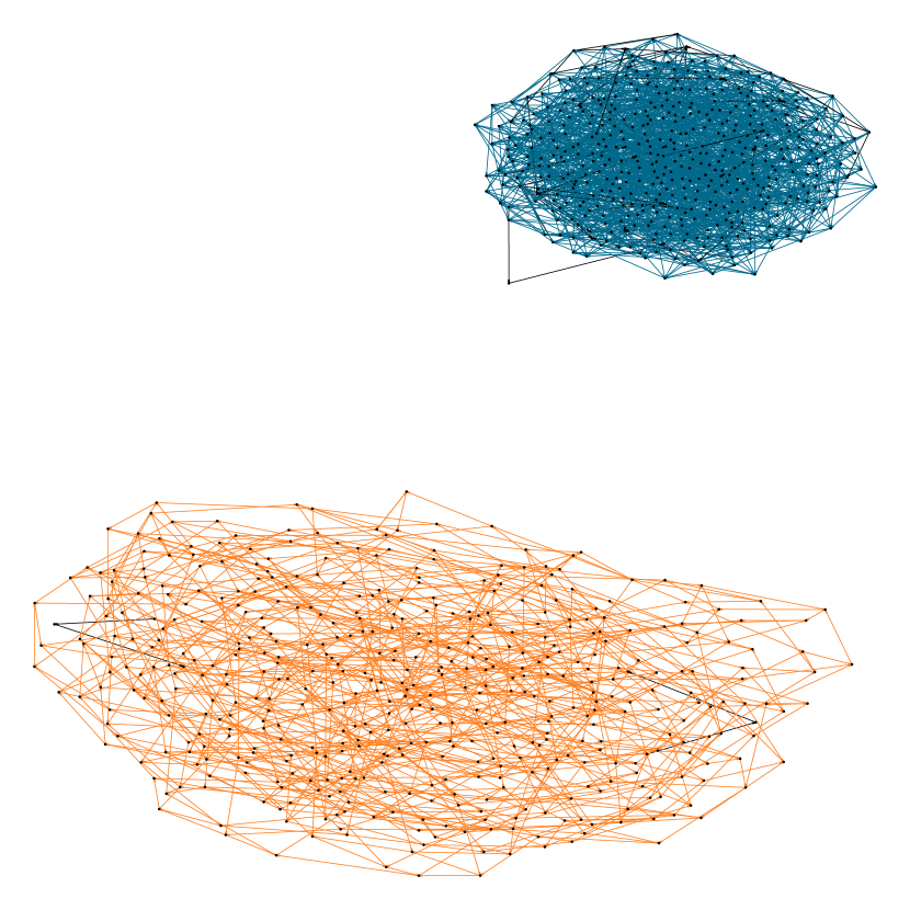
(a) $q=1$, $\rho_{q}=1$, $\hat{\rho}_{q}=0.99$.

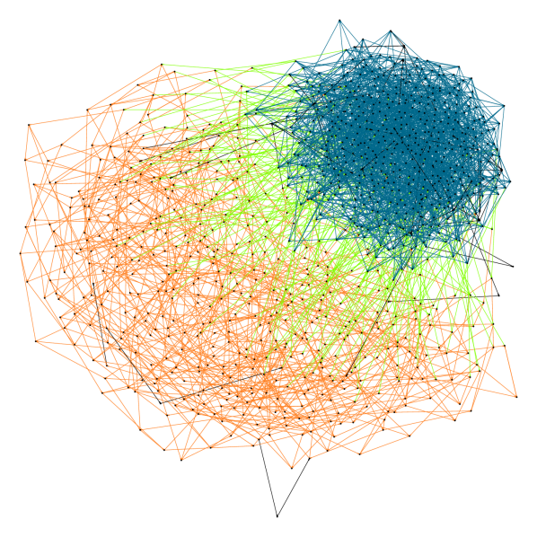
(b) $q=\frac{14}{15}$, $\rho_{q}=0.8$, $\hat{\rho}_{q}=0.79$.

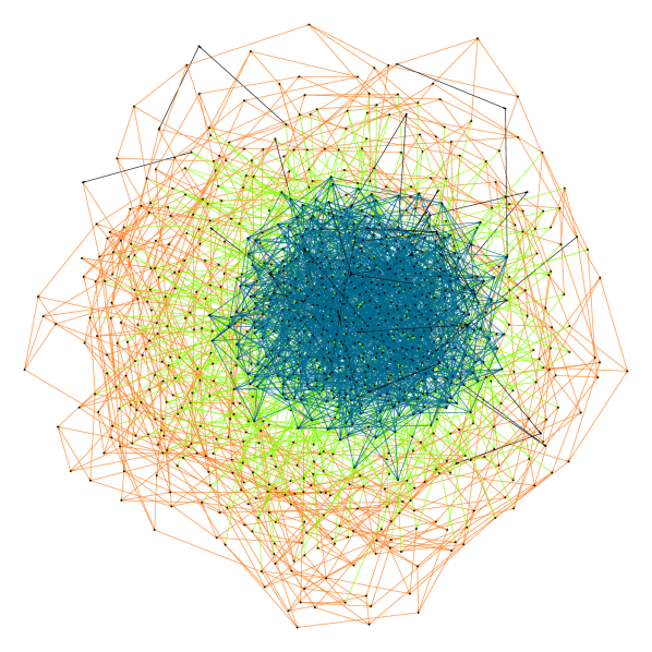
(c) $q=\frac{13}{15}$, $\rho_{q}=0.6$, $\hat{\rho}_{q}=0.6$.

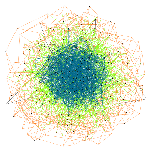
(d) $q=0.8$, $\rho_{q}=0.4$, $\hat{\rho}_{q}=0.39$.

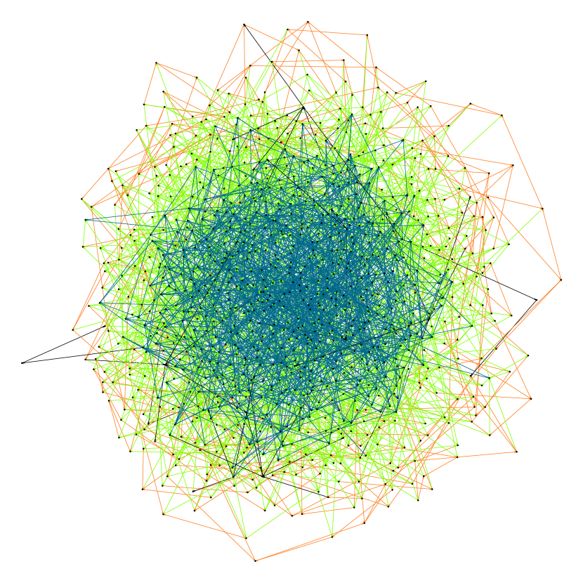
(e) $q=\frac{2}{3}$, $\rho_{q}=0$, $\hat{\rho}_{q}=0.01$.

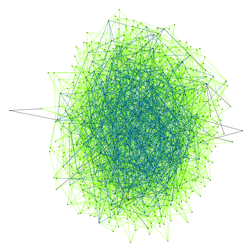
(f) $q=0.5$, $\rho_{q}=-0.5$, $\hat{\rho}_{q}=-0.49$.

Figure 4: All graphs were generated by our algorithm in Section 3 with $N=1000$, with the same node-type distribution $P_{0.5}={\rm diag}(0,0,0.5,0,0.5)$ but different edge-type distribution $Q_{q}$. Edges of type $(2,2)$ are colored orange, while edges of type $(4,4)$ are colored blue. Edges of types $(2,4)$ and $(4,2)$ are colored green. All other edges are colored black.

Note that the algorithm produces node-types different from $(2,2)$ and $(4,4)$ due to the modifications on nodes $\{N^{\prime}+1,\ldots,N\}$ with $N-N^{\prime}\ll N$ as $N\to\infty$. For better illustration we erase self-loops and multiple edges, and we do not show nodes of type $(0,0)$. To illustrate the differences between the six generated graphs we color edges of identical types the same as follows:

edges of type $$(2,2)$$ are orange,

edges of types $$(2,4) (4,2)$$ and are green,

$$\text{edges of type $(4,4)$ are blue},$$

and all other edges are colored black (which may arise by the construction and the erasure procedure).

We analyze the resulting empirical distributions $\hat{P}=(\hat{p}_{j,k})=({\mathcal{V}}_{j,k}/N)$ and $\hat{Q}_{q}=(\hat{q}_{k,j})=({\mathcal{E}}_{k,j}/{\mathcal{E}})$ for all six graphs in Figure 4. Let us first consider the graphs without having erased self-loops and multiple edges. For all simulations we have set $\delta=0.5+0.0001$ implying that $N-N^{\prime}=80$ nodes out of the total $1000$ do not have a bi-degree generated from $P$. This implies that the sum of the components of the difference $\hat{P}-\text{diag}(0,0,\hat{p}_{2,2},0,\hat{p}_{4,4})$ is at most $0.08$ for all generated graphs. For all the graphs in Figure 4 we observe empirically that the sum is at most $0.075$. Moreover, the differences $|\hat{p}_{2,2}-p_{2,2}|$ and $|\hat{p}_{4,4}-p_{4,4}|$ are both at most $0.043$ for all six graphs. For $\hat{Q}_{q}$ we have $|\hat{q}_{k,j}-q_{k,j}|\leq 0.02$ for all possible edge-types $(k,j)$ and all six graphs. From this we conclude that already for a comparably small graph of $N=1000$ nodes we obtain very accurate results (note that the results are exact for $N\to\infty$).

In Figure 4 we also present the values of the empirical assortativity coefficients $\hat{\rho}_{q}$. Note that they slightly deviate from the actual assortativity coefficients because of the randomness in the construction and the erasure procedure. Nevertheless, by Theorem 2.5 and by the continuous mapping theorem, the empirical assortativity coefficient $\hat{\rho}_{q}$ converges in probability to $\rho_{q}$ as $N\to\infty$. In Figure 5 we analyze how much $\hat{\rho}_{q}$ deviates from $\rho_{q}$ for the fixed distributions $P_{0.5}$ and $Q_{q}$ from above with $q=14/15$, so that $\rho_{q}=0.8$. For different values of $N$, we simulate $100$ (simple) graphs of size $N$ using the implementation of the algorithm provided in (1.1) with $\delta=0.5+0.0001$. Figure 5 illustrates that the convergence of $\hat{\rho}_{q}$ to the true value $\rho_{q}$ is reasonably fast, while we observe a bias for smaller values of $N$. Finally, Figure 5 indicates that the runtime of one graph simulation is approximately linear in $N$ for the given distributions $P_{0.5}$ and $Q_{14/15}$.

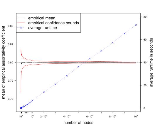
Figure 5: Mean of empirical assortativity coefficient with confidence bounds of one empirical standard deviation for different values of $N$ and $100$ simulations for each $N$ (left axis). Each cross indicates the average runtime in seconds for the simulation of a graph for fixed $N$ (right axis).

5 Proofs

We start with the proof of Lemma 3.1 which states that ${\mathbb{P}}[A_{N}]\to 1$ as $N\to\infty$.

Proof of Lemma 3.1. For each $k\in[K]_{1}$, $n_{k}^{+}$ has a binomial distribution with parameters $N^{\prime}$ and $p_{k}^{+}$. Therefore, by Chebyshev’s inequality,

$${\mathbb{P}}\left[\left|n_{k}^{+}-p_{k}^{+}N^{\prime}\right|>p_{k}^{+}N^{\delta}/2\right]~{}\leq~{}\frac{N^{\prime}p_{k}^{+}(1-p_{k}^{+})}{N^{2\delta}(p_{k}^{+})^{2}/4}~{}\to~{}0,\quad\text{as $N\to\infty$,}$$

since $\delta\in(1/2,1)$. Similarly, $\sum_{e=1}^{\lceil zN^{\prime\prime}\rceil}1_{\{k_{e}=k\}}$ has a binomial distribution with parameters $\lceil zN^{\prime\prime}\rceil$ and $q_{k}^{+}$. Therefore, by condition (C1), $\sum_{e=1}^{\lceil zN^{\prime\prime}\rceil}1_{\{k_{e}=k\}}/k$ has mean $q_{k}^{+}\lceil zN^{\prime\prime}\rceil/k=p_{k}^{+}\lceil zN^{\prime\prime}\rceil/z$ and its variance is of order $N^{\prime\prime}$. By Chebyshev’s inequality it follows that

$${\mathbb{P}}\left[\left|e_{k}^{+}-p_{k}^{+}N^{\prime\prime}\right|>p_{k}^{+}N^{\delta}/2\right]~{}\to~{}0,\quad\text{as $N\to\infty$.}$$

Similarly for $n_{j}^{-}$ and $e_{j}^{-}$, $j\in[J]_{1}$, using condition (C2). $\square$

Proof of Theorem 2.3. Choose $s\in{\mathbb{N}}$ fixed and let $u:({\mathbb{N}}_{0}\times{\mathbb{N}}_{0})^{s}\to[-H,H]$ be a function bounded by $H>0$. For $N\in{\mathbb{N}}$, denote by $(j_{1},k_{1}),\ldots,(j_{N},k_{N})$ the node-types generated by the algorithm in Section 3. Define $\big{(}(\tilde{j}_{1},\tilde{k}_{1}),\ldots,(\tilde{j}_{N},\tilde{k}_{N})\big{)}$, where $(\tilde{j}_{v},\tilde{k}_{v})=(j_{v},k_{v})$ for all $v=1,\ldots,N^{\prime}$, and $(\tilde{j}_{v},\tilde{k}_{v})$, $v=N^{\prime}+1,\ldots,N$, are independent random variables each having distribution $P$. By the triangle inequality we have

$$\left|{\mathbb{E}}\left[u((j_{v_{1}},k_{v_{1}}),\ldots,(j_{v_{s}},k_{v_{s}}))\right]-{\mathbb{E}}\left[u((j^{\prime}_{1},k^{\prime}_{1}),\ldots,(j^{\prime}_{s},k^{\prime}_{s}))\right]\right|$$

$$\leq~{}\left|{\mathbb{E}}\left[u((j_{v_{1}},k_{v_{1}}),\ldots,(j_{v_{s}},k_{v_{s}}))-u((\tilde{j}_{v_{1}},\tilde{k}_{v_{1}}),\ldots,(\tilde{j}_{v_{s}},\tilde{k}_{v_{s}}))\right]\right|$$

$$\hskip 28.45274pt+~{}\left|{\mathbb{E}}\left[u((\tilde{j}_{v_{1}},\tilde{k}_{v_{1}}),\ldots,(\tilde{j}_{v_{s}},\tilde{k}_{v_{s}}))-u((j^{\prime}_{1},k^{\prime}_{1}),\ldots,(j^{\prime}_{s},k^{\prime}_{s}))\right]\right|.$$

Since on $A_{N}$, $\big{(}(\tilde{j}_{v_{1}},\tilde{k}_{v_{1}}),\ldots,(\tilde{j}_{v_{s}},\tilde{k}_{v_{s}})\big{)}$ has the same distribution as $\big{(}(j^{\prime}_{1},k^{\prime}_{1}),\ldots,(j^{\prime}_{s},k^{\prime}_{s})\big{)}$, the second term on the right-hand side satisfies

$$\left|{\mathbb{E}}\left[u((\tilde{j}_{v_{1}},\tilde{k}_{v_{1}}),\ldots,(\tilde{j}_{v_{s}},\tilde{k}_{v_{s}}))-u((j^{\prime}_{1},k^{\prime}_{1}),\ldots,(j^{\prime}_{s},k^{\prime}_{s}))\right]\right|$$

$$\leq~{}\left|{\mathbb{E}}\left[\left.u((\tilde{j}_{v_{1}},\tilde{k}_{v_{1}}),\ldots,(\tilde{j}_{v_{s}},\tilde{k}_{v_{s}}))-u((j^{\prime}_{1},k^{\prime}_{1}),\ldots,(j^{\prime}_{s},k^{\prime}_{s}))\right|A_{N}\right]\right|+2H{\mathbb{P}}[A_{N}^{c}]$$

$$=~{}2H{\mathbb{P}}[A_{N}^{c}],$$

which converges to $0$ as $N\to\infty$ by Lemma 3.1. For the first term we have by the definition of the random variables $(\tilde{j}_{v},\tilde{k}_{v})$, $v=1,\ldots,N$,

$$\left|{\mathbb{E}}\left[u((j_{v_{1}},k_{v_{1}}),\ldots,(j_{v_{s}},k_{v_{s}}))-u((\tilde{j}_{v_{1}},\tilde{k}_{v_{1}}),\ldots,(\tilde{j}_{v_{s}},\tilde{k}_{v_{s}}))\right]\right|$$

$$=~{}\left|{\mathbb{E}}\left[\left(u((j_{v_{1}},k_{v_{1}}),\ldots,(j_{v_{s}},k_{v_{s}}))-u((\tilde{j}_{v_{1}},\tilde{k}_{v_{1}}),\ldots,(\tilde{j}_{v_{s}},\tilde{k}_{v_{s}}))\right)1_{\bigcup_{l=1}^{s}\left\{v_{l}\in\{N^{\prime}+1,\ldots,N\}\right\}}\right]\right|$$

$$\leq~{}2H\sum_{l=1}^{s}{\mathbb{P}}\left[v_{l}\in\{N^{\prime}+1,\ldots,N\}\right]~{}=~{}2Hs\frac{N-N^{\prime}}{N},$$

which converges to $0$ as $N\to\infty$ by the choice of $N^{\prime}$. The corresponding result for the edge-types follows by exactly the same arguments since, on event $A_{N}$, the number of generated edge-types having distribution $Q$ is $\lceil zN^{\prime\prime}\rceil$ and the number of artificially added edge-types is at most $K^{2}+J^{2}$, see Step 2 of the algorithm. $\square$

Proof of Theorem 2.4. Let $j\in[J]_{0}$, $k\in[K]_{0}$ and choose $\varepsilon>0$. For $N$ so large that $(N-N^{\prime})/N\leq\varepsilon/2$ we have

$${\mathbb{P}}\left[\left|\frac{1}{N}\sum_{v=1}^{N}1_{\{j_{v}=j,k_{v}=k\}}-p_{j,k}\right|>\varepsilon\right] \leq {\mathbb{P}}\left[\left.\frac{N-N^{\prime}}{N}+\left|\frac{1}{N}\sum_{v=1}^{N^{\prime}}1_{\{j_{v}=j,k_{v}=k\}}-p_{j,k}\right|>\varepsilon\right|A_{N}\right]+{\mathbb{P}}\left[A_{N}^{c}\right]$$

$$\leq {\mathbb{P}}\left[\left.\left|\sum_{v=1}^{N^{\prime}}1_{\{j_{v}=j,k_{v}=k\}}-p_{j,k}N\right|>N\varepsilon/2\right|A_{N}\right]+{\mathbb{P}}\left[A_{N}^{c}\right].$$

By Lemma 3.1 it remains to consider the first term on the right-hand side. By the triangle and Chebyshev’s inequality it follows that

$${\mathbb{P}}\left[\left.\left|\sum_{v=1}^{N^{\prime}}1_{\{j_{v}=j,k_{v}=k\}}-p_{j,k}N\right|>N\varepsilon/2\right|A_{N}\right] \leq \frac{N^{\prime}p_{j,k}(1-p_{j,k})}{{\mathbb{P}}\left[A_{N}\right]N^{2}\varepsilon^{2}/16}+{\mathbb{P}}\left[\left.(N-N^{\prime})p_{j,k}>N\varepsilon/4\right|A_{N}\right],$$

which converges to $0$ as $N\to\infty$ by Lemma 3.1. Similarly for the edge-types. $\square$

In order to prove Theorem 2.5, we first show that the expected number of self-loops and multiple edges arising from the construction in Section 3 is bounded in $N$.

Lemma 5.1.

Let $S_{N}$ be the number of self-loops and $M_{N}$ be the number of multiple edges of the graph generated by the algorithm in Section 3. There exists a finite constant $C>0$ such that

$${\mathbb{E}}\left[\left.S_{N}+M_{N}\right|A_{N}\right]~{}\leq~{}C.$$

Proof of Lemma 5.1. Let $v\in\{1,\ldots,N\}$ and denote by $s_{v}$ the number of edges $e$ with $e=\langle v,v\rangle$. Note that in order to have a self-loop $e=\langle v,v\rangle$, both ends of an edge of type $(k_{v},j_{v})$ have to be assigned to node $v$, see also Step 4 of the algorithm. Therefore, since there are $k_{v}$ edges leaving from $v$, we obtain upper bound

$${\mathbb{E}}[\left.S_{N}\right|A_{N}] = \sum_{v=1}^{N}{\mathbb{E}}[\left.s_{v}\right|A_{N}]~{}=~{}\sum_{v=1}^{N}{\mathbb{E}}\left[\left.k_{v}\frac{{\mathcal{E}}_{k_{v},j_{v}}}{{\mathcal{E}}_{k_{v}}^{+}}\frac{1}{{\mathcal{V}}_{j_{v}}^{-}}\right|A_{N}\right]~{}\leq~{}\sum_{v=1}^{N}{\mathbb{E}}\left[\left.\frac{k_{v}}{{\mathcal{V}}_{j_{v}}^{-}}\right|A_{N}\right].$$

Here, ${\mathcal{E}}_{k_{v}}^{+}$ denotes the number of generated edges $e=\langle v^{\prime},w\rangle$ with out-degree of $v^{\prime}$ being $k_{v}$ and ${\mathcal{V}}_{j_{v}}^{-}$ denotes the number of nodes having in-degree $j_{v}$. On event $A_{N}$, the number of nodes having in-degree $j_{v}$ is at least $\max\{1,p_{j_{v}}^{-}N^{\prime}-p_{j_{v}}^{-}N^{\delta}/2\}$. It follows that

$${\mathbb{E}}[\left.S_{N}\right|A_{N}] \leq \sum_{v=1}^{N}{\mathbb{E}}\left[\left.\frac{k_{v}}{\max\left\{1,p_{j}^{-}N^{\prime}-p_{j}^{-}N^{\delta}/2\right\}}\right|A_{N}\right]~{}\leq~{}\frac{NK}{\max\left\{1,\min_{j\in[J]_{1}}\left\{p_{j}^{-}N^{\prime}-p_{j}^{-}N^{\delta}/2\right\}\right\}}.$$

Since $z>0$, there exists $j\in[J]_{1}$ with $p_{j}^{-}>0$ and, hence, the right-hand side is bounded in $N$.

To bound the expectation of $M_{N}$, let $v\in\{1,\ldots,N\}$ and denote by $m_{v}$ the number of multiple edges leaving from node $v$. The probability that two distinct edges leaving from $v$ are arriving at the same node $w\neq v$ is at most

$$\frac{j_{w}(j_{w}-1)}{j_{w}{\mathcal{V}}_{j_{w}}^{-}\left(j_{w}{\mathcal{V}}_{j_{w}}^{-}-1\right)}1_{\{j_{w}\geq 2\}}.$$

It follows that

$${\mathbb{E}}[\left.M_{N}\right|A_{N}] = \sum_{v=1}^{N}{\mathbb{E}}[\left.m_{v}\right|A_{N}]~{}\leq~{}\sum_{v=1}^{N}\sum_{w=1}^{N}{\mathbb{E}}\left[\left.\binom{k_{v}}{2}\frac{j_{w}(j_{w}-1)}{j_{w}{\mathcal{V}}_{j_{w}}^{-}\left(j_{w}{\mathcal{V}}_{j_{w}}^{-}-1\right)}1_{\{j_{w}\geq 2\}}1_{\{k_{v}\geq 2\}}\right|A_{N}\right]$$

$$\leq \sum_{v=1}^{N}\sum_{w=1}^{N}{\mathbb{E}}\left[\left.\frac{k_{v}^{2}j_{w}^{2}}{2j_{w}{\mathcal{V}}_{j_{w}}^{-}\left(j_{w}{\mathcal{V}}_{j_{w}}^{-}-1\right)}1_{\{j_{w}\geq 2\}}1_{\{k_{v}\geq 2\}}\right|A_{N}\right].$$

Since $2j_{w}{\mathcal{V}}_{j_{w}}^{-}\left(j_{w}{\mathcal{V}}_{j_{w}}^{-}-1\right)\geq\left(j_{w}{\mathcal{V}}_{j_{w}}^{-}\right)^{2}$ for $j_{w}\geq 2$, it follows that

$${\mathbb{E}}[\left.M_{N}\right|A_{N}] \leq \sum_{v=1}^{N}\sum_{w=1}^{N}{\mathbb{E}}\left[\left.\frac{k_{v}^{2}}{\left({\mathcal{V}}_{j_{w}}^{-}\right)^{2}}1_{\{j_{w}\geq 2\}}1_{\{k_{v}\geq 2\}}\right|A_{N}\right].$$

Using that on $A_{N}$, the number of nodes having in-degree $j_{w}$ is at least $\max\{1,p_{j_{w}}^{-}N^{\prime}-p_{j_{w}}^{-}N^{\delta}/2\}$, it follows that

$${\mathbb{E}}[\left.M_{N}\right|A_{N}] \leq \frac{N^{2}K^{2}}{\max\left\{1,\min_{j\in[J]_{1}}\left\{p_{j}^{-}N^{\prime}-p_{j}^{-}N^{\delta}/2\right\}\right\}^{2}}.$$

The right-hand side is again bounded in $N$. This finishes the proof of Lemma 5.1. $\square$

Proof of Theorem 2.5. We first show that Theorem 2.4 holds true for the erased configuration graph. Let $S_{N}$ be the number of self-loops and let $M_{N}$ be the number of multiple edges generated by the algorithm. For $j\in[J]_{0}$ and $k\in[K]_{0}$ denote by ${\mathcal{V}}_{j,k}^{e}$ the number of constructed nodes of type $(j,k)$ after erasing all self-loops and multiple edges. Similarly we define ${\mathcal{E}}_{k,j}^{e}$ for $k\in[K]_{1}$ and $j\in[J]_{1}$. In order to prove that Theorem 2.4 holds true for the erased configuration graph, we show that for any $\varepsilon>0$,

$$\lim_{N\to\infty}{\mathbb{P}}\left[\sum_{j\in[J]_{0},k\in[K]_{0}}\left|\frac{{\mathcal{V}}^{e}_{j,k}}{N}-p_{j,k}\right|\geq\varepsilon\quad\text{ or }\quad\sum_{k\in[K]_{1},j\in[J]_{1}}\left|{\mathcal{E}}^{e}_{k,j}-q_{k,j}{\mathcal{E}}^{e}\right|\geq\varepsilon{\mathcal{E}}^{e}\right]~{}=~{}0,$$ (5.1)

where ${\mathcal{E}}^{e}$ denotes the total number of edges in the erased configuration graph (which could be equal to $0$ if all edges of the constructed graph are self-loops). Let $\varepsilon>0$ and choose $j\in[J]_{0}$ and $k\in[K]_{0}$. We have

$${\mathbb{P}}\left[\left|\frac{{\mathcal{V}}^{e}_{j,k}}{N}-p_{j,k}\right|\geq\varepsilon\right]~{}\leq~{}{\mathbb{P}}\left[\left|\frac{{\mathcal{V}}^{e}_{j,k}-{\mathcal{V}}_{j,k}}{N}\right|\geq\varepsilon/2\right]+{\mathbb{P}}\left[\left|\frac{{\mathcal{V}}_{j,k}}{N}-p_{j,k}\right|\geq\varepsilon/2\right].$$

The second term on the right-hand side converges to $0$ as $N\to\infty$ by Theorem 2.4. For the first term, note that

$${\mathbb{P}}\left[\left|\frac{{\mathcal{V}}^{e}_{j,k}-{\mathcal{V}}_{j,k}}{N}\right|\geq\varepsilon/2\right]~{}\leq~{}{\mathbb{P}}\left[\sum_{v=1}^{N}\left|1_{\{j_{v}^{e}=j,k_{v}^{e}=k\}}-1_{\{j_{v}=j,k_{v}=k\}}\right|\geq\varepsilon N/2\right],$$

where $(j_{v}^{e},k^{e}_{v})$ denotes the type of node $v$ in the erased configuration graph. Denote by $s_{v}$ the number of self-loops attached to $v$. Denote by $m_{v}^{+}$ the number of multiple edges leaving from $v$ and denote by $m_{v}^{-}$ the number of multiple edges arriving at $v$. Note that $j_{v}^{e}=j_{v}$ if and only if $s_{v}+m^{-}_{v}=0$, and similarly $k_{v}^{e}=k_{v}$ if and only if $s_{v}+m^{+}_{v}=0$. We therefore have that

$$1_{\{j_{v}^{e}=j,k_{v}^{e}=k\}}-1_{\{j_{v}=j,k_{v}=k\}} = 1_{\{s_{v}+m_{v}^{-}>0\text{ or }s_{v}+m_{v}^{+}>0\}}\left(1_{\{j_{v}^{e}=j,k_{v}^{e}=k\}}-1_{\{j_{v}=j,k_{v}=k\}}\right)$$

$$= 1_{\{s_{v}+m_{v}>0\}}\left(1_{\{j_{v}^{e}=j,k_{v}^{e}=k\}}-1_{\{j_{v}=j,k_{v}=k\}}\right),$$

where we set $m_{v}=m_{v}^{+}+m_{v}^{-}$. Hence,

$${\mathbb{P}}\left[\left|\frac{{\mathcal{V}}^{e}_{j,k}-{\mathcal{V}}_{j,k}}{N}\right|\geq\varepsilon/2\right] \leq {\mathbb{P}}\left[\sum_{v=1}^{N}1_{\{s_{v}+m_{v}>0\}}\geq\varepsilon N/2\right]~{}\leq~{}{\mathbb{P}}\left[\sum_{v=1}^{N}(s_{v}+m_{v})\geq\varepsilon N/2\right].$$

It follows by Markov’s inequality, Lemma 3.1 and Lemma 5.1 that

$${\mathbb{P}}\left[\left|\frac{{\mathcal{V}}^{e}_{j,k}-{\mathcal{V}}_{j,k}}{N}\right|\geq\varepsilon/2\right] \leq {\mathbb{P}}\left[S_{N}+2M_{N}\geq N\varepsilon/2\right]~{}\leq~{}\frac{{\mathbb{E}}\left[\left.S_{N}+2M_{N}\right|A_{N}\right]}{N\varepsilon/2}+{\mathbb{P}}\left[A_{N}^{c}\right]~{}\to~{}0,\quad\text{ as $N\to\infty$.}$$

We now prove the same result for the edge-types under the conditional probability, conditional given $A_{N}$, which is enough due to Lemma 3.1. Note that on event $A_{N}$ the number of generated edges ${\mathcal{E}}$ is at least $zN^{\prime\prime}$, see Step 1 of the algorithm. It follows by Markov’s inequality and Lemma 5.1, and since ${\mathcal{E}}-{\mathcal{E}}^{e}=S_{N}+M_{N}$, that for every $\eta>0$,

$${\mathbb{P}}\left[\left.\left|\frac{{\mathcal{E}}^{e}}{{\mathcal{E}}}-1\right|\geq\eta\;\right|A_{N}\right]~{}=~{}{\mathbb{P}}\left[\left.\frac{S_{N}+M_{N}}{{\mathcal{E}}}\geq\eta\;\right|A_{N}\right]~{}\leq~{}{\mathbb{P}}\left[\left.S_{N}+M_{N}\geq zN^{\prime\prime}\eta\;\right|A_{N}\right]~{}\to~{}0,$$ (5.2)

as $N\to\infty$. Note that for fixed $k\in[K]_{1}$ and $j\in[J]_{1}$,

$${\mathbb{P}}\left[\left.\left|{\mathcal{E}}^{e}_{k,j}-q_{k,j}{\mathcal{E}}^{e}\right|\geq\varepsilon{\mathcal{E}}^{e}\;\right|A_{N}\right] \leq {\mathbb{P}}\left[\left.\left|{\mathcal{E}}^{e}_{k,j}-{\mathcal{E}}_{k,j}\right|\geq\varepsilon{\mathcal{E}}^{e}/2\;\right|A_{N}\right]+{\mathbb{P}}\left[\left.\left|{\mathcal{E}}_{k,j}-q_{k,j}{\mathcal{E}}^{e}\right|\geq\varepsilon{\mathcal{E}}^{e}/2\;\right|A_{N}\right].$$

For the second term on the right-hand side we have

$${\mathbb{P}}\left[\left.\left|{\mathcal{E}}_{k,j}-q_{k,j}{\mathcal{E}}^{e}\right|\geq\varepsilon{\mathcal{E}}^{e}/2\;\right|A_{N}\right] = {\mathbb{P}}\left[\left.\left|\frac{{\mathcal{E}}_{k,j}}{{\mathcal{E}}}-\frac{{\mathcal{E}}-S_{N}-M_{N}}{{\mathcal{E}}}q_{k,j}\right|\geq\frac{{\mathcal{E}}^{e}}{{\mathcal{E}}}\varepsilon/2\;\right|A_{N}\right]$$

$$\leq~{}{\mathbb{P}}\left[\left.\left|\frac{{\mathcal{E}}_{k,j}}{{\mathcal{E}}}-q_{k,j}\right|\geq\frac{{\mathcal{E}}^{e}}{{\mathcal{E}}}\varepsilon/4\;\right|A_{N}\right]+{\mathbb{P}}\left[\left.\left(S_{N}+M_{N}\right)q_{k,j}\geq{\mathcal{E}}^{e}\varepsilon/4\;\right|A_{N}\right]$$

$$\leq~{}{\mathbb{P}}\left[\left.\left|\frac{{\mathcal{E}}_{k,j}}{{\mathcal{E}}}-q_{k,j}\right|\geq\frac{{\mathcal{E}}^{e}}{{\mathcal{E}}}\varepsilon/4\;\right|A_{N}\right]+{\mathbb{P}}\left[\left.S_{N}+M_{N}\geq\frac{zN^{\prime\prime}\varepsilon/4}{q_{k,j}+\varepsilon/4}\;\right|A_{N}\right],$$

where in the last step we used that ${\mathcal{E}}^{e}={\mathcal{E}}-(S_{N}+M_{N})\geq zN^{\prime\prime}-(S_{N}+M_{N})$. By Theorem 2.4, (5.2) and Lemma 5.1, the right-hand side converges to $0$ as $N\to\infty$. To bound the first term, note that the erasure procedure changes the number of edges of type $(k,j)$ because such edges may get erased, but also because an erased edge $e=\langle v,w\rangle$ changes the types of unerased edges that are leaving from node $v$ or that are arriving at node $w$. It follows that

$${\mathbb{P}}\left[\left.\left|{\mathcal{E}}^{e}_{k,j}-{\mathcal{E}}_{k,j}\right|\geq\varepsilon{\mathcal{E}}^{e}/2\;\right|A_{N}\right]~{}\leq~{}{\mathbb{P}}\left[\left.S_{N}+M_{N}+\sum_{e=1}^{{\mathcal{E}}^{e}}\left|1_{\{k^{e}_{e}=k,j_{e}^{e}=j\}}-1_{\{k_{e}=k,j_{e}=j\}}\right|\geq\varepsilon{\mathcal{E}}^{e}/2\;\right|A_{N}\right],$$

where $(k^{e}_{e},j_{e}^{e})$ denotes the type of edge $e$ in the erased configuration graph. For an edge $e=\langle v,w\rangle$ we have $k_{e}^{e}=k_{e}$ if and only if $s_{v}+m_{v}^{+}=0$, and similarly $j_{e}^{e}=j_{e}$ if and only if $s_{w}+m_{w}^{-}=0$. Therefore, for $e=\langle v,w\rangle$,

$$1_{\{k^{e}_{e}=k,j_{e}^{e}=j\}}-1_{\{k_{e}=k,j_{e}=j\}} = 1_{\{s_{v}+m_{v}^{+}>0\text{ or }s_{w}+m_{w}^{-}>0\}}\left(1_{\{k^{e}_{e}=k,j_{e}^{e}=j\}}-1_{\{k_{e}=k,j_{e}=j\}}\right)$$

$$= 1_{\{s_{e}+m_{e}>0\}}\left(1_{\{k^{e}_{e}=k,j_{e}^{e}=j\}}-1_{\{k_{e}=k,j_{e}=j\}}\right),$$

where we set $s_{e}=s_{v}+s_{w}$ and $m_{e}=m_{v}^{+}+m_{w}^{-}$. It follows that

$${\mathbb{P}}\left[\left.\left|{\mathcal{E}}^{e}_{k,j}-{\mathcal{E}}_{k,j}\right|\geq\varepsilon{\mathcal{E}}^{e}/2\;\right|A_{N}\right] \leq {\mathbb{P}}\left[\left.S_{N}+M_{N}+\sum_{e=1}^{{\mathcal{E}}^{e}}1_{\{s_{e}+m_{e}>0\}}\geq\varepsilon{\mathcal{E}}^{e}/2\;\right|A_{N}\right]$$

$$\leq~{}{\mathbb{P}}\left[\left.S_{N}+M_{N}+\sum_{v=1}^{N}\left(k_{v}1_{\{s_{v}+m^{+}_{v}>0\}}+j_{v}1_{\{s_{v}+m_{v}^{-}>0\}}\right)\geq{\mathcal{E}}^{e}\varepsilon/2\;\right|A_{N}\right]$$

$$\leq~{}{\mathbb{P}}\left[\left.S_{N}+M_{N}+K(S_{N}+M_{N})+J(S_{N}+M_{N})\geq{\mathcal{E}}^{e}\varepsilon/2\;\right|A_{N}\right],$$

which converges to $0$ as $N\to\infty$ by Lemma 5.1 and the fact that ${\mathcal{E}}^{e}={\mathcal{E}}-(S_{N}+M_{N})\geq zN^{\prime\prime}-(S_{N}+M_{N})$. This finally proves (5.1).

We now prove that Theorem 2.3 holds true for the erased configuration graph. Denote by ${\mathcal{V}}_{\rm mod}$ the set of nodes whose types have been changed due to the erasure procedure. For the probability that a uniformly chosen node $v$ belongs to $\{N^{\prime}+1,\ldots,N\}\cup{\mathcal{V}}_{\rm mod}$ we have

$${\mathbb{P}}\left[v\in\{N^{\prime}+1,\ldots,N\}\cup{\mathcal{V}}_{\rm mod}\right] = {\mathbb{E}}\left[\frac{\left|\{N^{\prime}+1,\ldots,N\}\cup{\mathcal{V}}_{\rm mod}\right|}{N}\right]~{}\leq~{}{\mathbb{E}}\left[\frac{N-N^{\prime}+S_{N}+2M_{N}}{N}\right].$$

Since the graph returned by the algorithm in case event $A_{N}$ does not hold has no self-loops or multiple edges, see Step 5, it follows that

$${\mathbb{P}}\left[v\in\{N^{\prime}+1,\ldots,N\}\cup{\mathcal{V}}_{\rm mod}\right]~{}\leq~{}{\mathbb{E}}\left[\left.\frac{N-N^{\prime}+S_{N}+2M_{N}}{N}\right|A_{N}\right]+\frac{N-N^{\prime}}{N},$$

which converges to $0$ as $N\to\infty$ by Lemma 5.1. Going through the proof of Theorem 2.3, we see that this observation is enough to conclude that the types of $s\in{\mathbb{N}}$ randomly chosen nodes of the erased configuration graph converge in distribution to a sequence of $s$ independent random variables each having distribution $P$ as $N\to\infty$. To prove the same result for the edge-types of the erased configuration graph, note that it may happen that all edges of the graph generated by the algorithm of Section 3 are self-loops, i.e. ${\mathcal{E}}^{e}=0$. In this case the edge set is empty for the erased configuration graph and we define “the type of a randomly chosen edge” to be identical to $(1,1)$ if event $\{{\mathcal{E}}^{e}=0\}$ occurs, and we define it to be as usual if event $\{{\mathcal{E}}^{e}=0\}$ does not occur. Nevertheless, the probability of event $\{{\mathcal{E}}^{e}=0\}$ converges to $0$ as $N\to\infty$ by Lemma 3.1 and (5.2) above. Therefore, using similar arguments as above for the node-types, we conclude that the types of $s\in{\mathbb{N}}$ randomly chosen edges of the erased configuration graph converge in distribution to a sequence of $s$ independent random variables each having distribution $Q$ as $N\to\infty$. $\square$

Appendix A Variations of edge-types

We have defined assortativity through edge-types, which, for an edge $e=\langle v,w\rangle$ connecting node $v$ to node $w$, is defined to be the tuple $(k_{e},j_{e})$ with $k_{e}$ denoting the out-degree of $v$ and $j_{e}$ denoting the in-degree of $w$. There are three other possibilities to define the type of an edge $e$, for instance, by the tuple $(k_{e},k^{\prime}_{e})$ with $k_{e}$ and $k^{\prime}_{e}$ denoting the out-degree of $v$ and $w$, respectively. We briefly explain how we need to modify the presented algorithm in Section 3 when redefining the type of an edge as above. In the same spirit one can then construct algorithms for the remaining two definitions of edge-types. Results as in Lemma 3.1 and Theorems 2.3–2.5 can also be proven using the new definition of edge-types.

Define the type of an edge $e=\langle v,w\rangle$ by the tuple $(k_{e},k^{\prime}_{e})$ with $k_{e}$ and $k^{\prime}_{e}$ denoting the out-degree of node $v$ and $w$, respectively. In view of conditions (C1) and (C2) the corresponding edge-type distribution $Q=(q_{k,k^{\prime}})$ with marginal distributions $(q_{k}^{l})_{k\in[K]_{1}}$ and $(q_{k^{\prime}}^{r})_{k^{\prime}\in[K]_{0}}$ then needs to satisfy, for given node-type distribution $P$ with mean degree $z>0$,

$$q_{k}^{l}~{}=~{}kp_{k}^{+}/z,\quad k\in[K]_{1},\qquad\text{and}\qquad q_{k^{\prime}}^{r}~{}=~{}\sum_{j\in[J]_{1}}jp_{j,k^{\prime}}/z,\quad k^{\prime}\in[K]_{0}.$$ (A.1)

Here, superscript “$l$” refers to node $v$ of the edge $e=\langle v,w\rangle$ and superscript “$r$” to node $w$. Condition (A.1) is justified by counting nodes and edges of corresponding types in a given graph. For instance, note that for every node of type $(j,k^{\prime})$, $j\in[J]_{1}$ and $k^{\prime}\in[K]_{0}$, we have $j$ edges $e=\langle v,w\rangle$ with out-degree of $w$ being $k^{\prime}$.

We now describe a modification of the algorithm in Section 3 to construct graphs corresponding to the new distribution $Q$. Choose $N\in{\mathbb{N}}$ so large that there exists $N^{\prime}\in{\mathbb{N}}$ with $N=N^{\prime}+2(1+z)\left\lceil N^{\delta}\right\rceil+K^{2}$, and set $N^{\prime\prime}=N^{\prime}+\left\lceil N^{\delta}\right\rceil$.

1. Step 1. Assign to each node $v=1,\ldots,N^{\prime}$ independently a node-type $(j_{v},k_{v})$ according to distribution $P$. Generate edges $e=1,\ldots,\lceil zN^{\prime\prime}\rceil$ having independent edge-types $(k_{e},k^{\prime}_{e})$ according to distribution $Q$, independently of the node-types. Define

   $$n_{k}^{l} = \sum_{v=1}^{N^{\prime}}1_{\{k_{v}=k\}}\quad\text{ and }\quad e_{k}^{l}~{}=~{}\left\lceil\frac{1}{k}\sum_{e=1}^{\lceil zN^{\prime\prime}\rceil}1_{\{k_{e}=k\}}\right\rceil\quad\text{ for all $k\in[K]_{1}$};$$

   $$n_{k^{\prime}}^{r} = \sum_{j=1}^{J}j\sum_{v=1}^{N^{\prime}}1_{\{j_{v}=j,\,k_{v}=k^{\prime}\}}\quad\text{ and }\quad e_{k^{\prime}}^{r}~{}=~{}\sum_{e=1}^{\lceil zN^{\prime\prime}\rceil}1_{\{k^{\prime}_{e}=k^{\prime}\}}\quad\text{ for all $k^{\prime}\in[K]_{0}$}.$$

   Let $A_{N}$ be the event on which we have, set $p_{k^{\prime}}^{r}=\sum_{j=1}^{J}jp_{j,k^{\prime}}$,

   $$\left|n_{k}^{l}-p_{k}^{+}N^{\prime}\right|\leq p_{k}^{+}N^{\delta}/2 \left|e_{k}^{l}-p_{k}^{+}N^{\prime\prime}\right|\leq p_{k}^{+}N^{\delta}/2\quad\text{ for all $k\in[K]_{1}$};$$ and

   $$\left|n_{k^{\prime}}^{r}-p_{k^{\prime}}^{r}N^{\prime}\right|\leq p_{k^{\prime}}^{r}N^{\delta}/2 \left|e_{k^{\prime}}^{r}-p_{k^{\prime}}^{r}N^{\prime\prime}\right|\leq p_{k^{\prime}}^{r}N^{\delta}/2\quad\text{ for all $k^{\prime}\in[K]_{0}$}.$$ and

   Only accept Step 1 if event $A_{N}$ occurs and proceed to Step 2, otherwise return a graph containing at least one edge. Observe that by the relation between $N^{\prime}$ and $N^{\prime\prime}$ we have, on $A_{N}$, $n_{k}^{l}-e_{k}^{l}\leq 0$ for all $k\in[K]_{1}$ and $n_{k^{\prime}}^{r}-e_{k^{\prime}}^{r}\leq 0$ for all $k^{\prime}\in[K]_{0}$.

2. Steps 2 and 3. If the number of generated edges $e=\langle v,w\rangle$ with out-degree of $v$ being $k\in[K]_{1}$ is not a multiple of $k$, we add the corresponding number of edges of type $(k,0)$ and nodes of type $(1,0)$. Additionally, we add $e_{k}^{l}-n_{k}^{l}\geq 0$ nodes of type $(0,k)$, i.e. we finally obtain that the number of nodes with out-degree $k$ corresponds to the number of such nodes needed for the edges $e=\langle v,w\rangle$ with out-degree of $v$ being $k$.

   Note that $n_{k^{\prime}}^{r}$ is the sum of in-degrees of all nodes generated in Step 1 having out-degree $k^{\prime}\in[K]_{0}$, which is, since $e_{k^{\prime}}^{r}-n_{k^{\prime}}^{r}\geq 0$, eventually strictly less than $e_{k^{\prime}}^{r}$. Therefore, we add $e_{k^{\prime}}^{r}-n_{k^{\prime}}^{r}$ nodes of type $(1,k^{\prime})$, and for each such node we add an additional node of type $(k^{\prime},0)$. The node of type $(k^{\prime},0)$ is only needed if $k^{\prime}\geq 1$, because for each added node of type $(1,k^{\prime})$ we additionally add $k^{\prime}$ edges of type $(k^{\prime},0)$. Note that instead of adding a node of type $(k^{\prime},0)$ we could also add $k^{\prime}$ nodes of type $(1,0)$.

3. Step 4. For each $k\in[K]_{1}$, assign to each node having out-degree $k$ exactly $k$ uniformly chosen edges $e$ of type $(k_{e},k^{\prime}_{e})$ with $k_{e}=k$. For each $k^{\prime}\in[K]_{0}$, assign to every node $v$ of type $(j_{v},k_{v})$ with $k_{v}=k^{\prime}$ exactly $j_{v}$ uniformly chosen edges $e$ of type $(k_{e},k^{\prime}_{e})$ with $k^{\prime}_{e}=k^{\prime}$. Return the constructed graph.

Following this modified algorithm, the total number of nodes we add in Steps 2 and 3 is at most, on event $A_{N}$,

$$\sum_{k=1}^{K}\left(k-1+(e_{k}^{l}-n_{k}^{l})\right)+\sum_{k^{\prime}=0}^{K}(e_{k^{\prime}}^{r}-n_{k^{\prime}}^{r})\left(1+1\right)~{}\leq~{}K^{2}+2\lceil N^{\delta}\rceil+2z\lceil N^{\delta}\rceil.$$

This implies that we have sufficiently many undetermined nodes $N-N^{\prime}$ to which we can assign corresponding node-types. Moreover, the total number of edges we add in Steps 2 and 3 is at most, on event $A_{N}$,

$$\sum_{k=1}^{K}\left(k-1\right)+\sum_{k^{\prime}=0}^{K}k^{\prime}(e_{k^{\prime}}^{r}-n_{k^{\prime}}^{r})~{}\leq~{}K^{2}+zK\lceil N^{\delta}\rceil.$$

Remark A.1.

Note that when considering a variation of edge-types with corresponding distribution $Q$ satisfying (A.1) or variations thereof, then the marginal distributions of $Q$ are determined by the distribution $P$. Therefore, the discussion in the beginning of Section 4 carries over also for variations of edge-types.

References

• [1] Kevin E. Bassler, Charo I. Del Genio, Péter L. Erdős, István Miklós, and Zoltán Toroczkai. Exact sampling of graphs with prescribed degree correlations. New Journal of Physics, 17(August):083052, 18, 2015.
• [2] Morten L. Bech and Enghin Atalay. The topology of the federal funds market. Physica A: Statistical Mechanics and its Applications, 389(22):5223 – 5246, 2010.
• [3] Mindaugas Bloznelis, Jerzy Jaworski, and Valentas Kurauskas. Assortativity and clustering of sparse random intersection graphs. Electronic Journal of Probability, 18:no. 38, 24, 2013.
• [4] Béla Bollobás. A probabilistic proof of an asymptotic formula for the number of labelled regular graphs. European Journal of Combinatorics, 1(4):311–316, 1980.
• [5] Béla Bollobás. Random Graphs, volume 73 of Cambridge Studies in Advanced Mathematics. Cambridge University Press, Cambridge, second edition, 2001.
• [6] Ningyuan Chen and Mariana Olvera-Cravioto. Directed random graphs with given degree distributions. Stochastic Systems, 3(1):147–186, 2013.
• [7] Rama Cont, Amal Moussa, and Edson B. Santos. Network structure and systemic risk in banking systems. In Handbook of Systemic Risk, pages 327–367. Cambridge University Press, New York, 2013.
• [8] Rick Durrett. Random Graph Dynamics. Cambridge Series in Statistical and Probabilistic Mathematics. Cambridge University Press, Cambridge, 2007.
• [9] Paul Erdős and Alfréd Rényi. On random graphs. I. Publicationes Mathematicae Debrecen, 6:290–297, 1959.
• [10] Edgar N. Gilbert. Random graphs. Annals of Mathematical Statistics, 30:1141–1144, 1959.
• [11] Thomas R. Hurd. The construction and properties of assortative configuration graphs, 2015. Available at http://arxiv.org/abs/1512.03084.
• [12] Thomas R. Hurd. Contagion! The Spread of Systemic Risk in Financial Networks. SpringerBriefs in Quantitative Finance. Springer International Publishing, 2016.
• [13] Thomas R. Hurd and James P. Gleeson. A framework for analyzing contagion in banking networks, October 2011. Available at http://arxiv.org/abs/1110.4312.
• [14] Nelly Litvak and Remco van der Hofstad. Uncovering disassortativity in large scale-free networks. Physical Review E. Statistical, Nonlinear, and Soft Matter Physics, 87:022801, Feb 2013.
• [15] Alexander J. McNeil, Rüdiger Frey, and Paul Embrechts. Quantitative Risk Management: Concepts, Techniques and Tools. Princeton Series in Finance. Princeton University Press, Princeton, NJ, revised edition, 2015.
• [16] Mark E. J. Newman. Assortative mixing in networks. Physical Review Letters, 89:208701, Oct 2002.
• [17] Mark E. J. Newman. Mixing patterns in networks. Physical Review E. Statistical, Nonlinear, and Soft Matter Physics, 67(2):026126, 2003.
• [18] Kimmo Soramäki, Morten L. Bech, Jeffrey Arnold, Robert J. Glass, and Walter E. Beyeler. The topology of interbank payment flows. Physica A: Statistical Mechanics and its Applications, 379(1):317 – 333, 2007.
• [19] Isabelle Stanton and Ali Pinar. Constructing and sampling graphs with a prescribed joint degree distribution. ACM Journal of Experimental Algorithmics, 17:Article 3.5, 25, 2012.
• [20] Remco van der Hofstad. Random Graphs and Complex Networks. Vol. II. Preprint, available at http://www.win.tue.nl/~rhofstad/NotesRGCNII.pdf, 2014.
• [21] Remco van der Hofstad. Random Graphs and Complex Networks, volume 1. Cambridge University Press, Cambridge, 11 2016.
• [22] Remco van der Hofstad, Gerard Hooghiemstra, and Piet Van Mieghem. Distances in random graphs with finite variance degrees. Random Structures & Algorithms, 27(1):76–123, 2005.
• [23] Pim van der Hoorn and Nelly Litvak. Convergence of rank based degree-degree correlations in random directed networks. Moscow Journal of Combinatorics and Number Theory, 4(4):45–83, 2014.
• [24] Nicholas C. Wormald. Differential equations for random processes and random graphs. The Annals of Applied Probability, 5(4):1217–1235, 1995.