Schreier graphs of Grigorchuk’s group and a subshift associated to a non-primitive substitution

Abstract.

There is a recently discovered connection between the spectral theory of Schrö-dinger operators whose potentials exhibit aperiodic order and that of Laplacians associated with actions of groups on regular rooted trees, as Grigorchuk’s group of intermediate growth. We give an overview of corresponding results, such as different spectral types in the isotropic and anisotropic cases, including Cantor spectrum of Lebesgue measure zero and absence of eigenvalues. Moreover, we discuss the relevant background as well as the combinatorial and dynamical tools that allow one to establish the afore-mentioned connection. The main such tool is the subshift associated to a substitution over a finite alphabet that defines the group algebraically via a recursive presentation by generators and relators.

Introduction

The study of spectra of graphs associated with finitely generated groups, such as Cayley graphs or Schreier graphs (natural analogues of Cayley graphs associated to not necessarily free group actions) has a long history and is related to many problems in modern mathematics. Still, very little is known about the dependence of the spectrum of the Laplacian on the choice of generators in the group and on the weight on these generators. In the recent paper [40] we addressed the issue of dependence on the weights on generators in the example of Grigorchuk’s group of intermediate growth. More specifically, we determined the spectral type of the Laplacian on the Schreier graphs describing the action of Grigorchuk’s group on the boundary of the infinite binary tree and showed that it is different in the isotropic and anisotropic cases. In fact, the spectrum is shown to be a Cantor set of Lebesgue measure zero in the anisotropic case, whereas, as has been known for a long time, it consists of one or two intervals in the isotropic case. Moreover, we showed almost surely (with respect to a natural measure on the boundary of the tree) the absence of eigenvalues for the Laplacians in question.

Our investigation in [40] provides (and relies on) a surprising link between discrete Schrödinger operators with aperiodic order and the substitutional dynamics arising from a presentation of the group by generators and relators.

The purpose of the present paper is two-fold. Firstly, we want to survey the spectral theoretic results of [40]. Secondly, we want to put these results in wider perspective by discussing the background on aperiodic order in dimension one. In this context we present a discussion of subshifts and aperiodic order in Section 1 and of Schrödinger operators arising in models of (dis)ordered solids in Section 2.

We also continue our study of the substitution that is instrumental for the results in [40]. It first appeared in 1985 in the presentation of Grigorchuk’s group by generators and relators found by Lysenok [66] (such infinite recursive presentations are now called L-presentations). A remarkable fact is that the same substitution also describes basic dynamical properties of the group. Here we review its combinatorial properties and carry out a detailed study of the factor map to its maximal equicontinuous factor, which is the binary odometer. This factor map is proven to be one-to-one everywhere except on three orbits. This in turn can be linked to the phenomenon of pure point diffraction which is at the core of aperiodic order. All these discussions concerning the substitution are contained in Section 3.

The necessary background from graphs and dynamical systems is discussed in Section 4 and basics on Grigorchuk’s group and its Schreier graphs can be found in Section 5.

The connection between Schrödinger operators and Laplacians on Schreier graphs revealed in [40] (and reviewed in Sections 6 and 7) can also be used to show that the Kesten-von-Neuman trace and the integrated density of states agree. This seems to be somewhat folklore. We provide a proof in Section 8.

Our approach can certainly be carried out for various further families of groups generalizing Grigorchuk’s group. In particular, our results fully extend to a larger family of self-similar groups acting on the infinite binary tree considered by Sunic in [76], as well as to similar families of self-similar groups acting on regular rooted trees of arbitrary degrees that also have linear Schreier graphs for their action on the boundary of the tree. Moreover, each of these self-similar groups belongs to an uncountable family of groups parametrized by sequences in a certain finite alphabet, in the same way as Grigorchuk’s group belongs to the family of groups $(G_{\omega})_{\omega\in\{0,1,2\}^{\bf N}}$ constructed by the first named author in [37]. The Schreier graphs of the groups in the same family look the same, but their labelling by generators, and thus their spectra, depend on the sequence $\omega$. The associated subshifts are also different, in particular, they don’t have to come from a substitution in the case when the corresponding group is not self-similar. This more general setup will be considered in a separate paper.

Acknowledgments. R. G. was partially supported by the NSF grant DMS-1207669, by ERC AG COMPASP and by the NSA grant H98230-15-1-0328. The authors acknowledge support of the Swiss National Science Foundation. Part of this research was carried out while D.L. and R. G. were visiting the Department of mathematics of the University of Geneva. The hospitality of the department is gratefully acknowledged. The authors also thank Fabien Durand and Ian Putnam for most enlightening discussions concerning the material gathered in Section 3.7, Yaroslav Vorobets for allowing them to use his figures $3$ and $4$ and Olga Klimecki for help in preparing figure $1$. Finally, the authors would like to thank the anonymous referee for a very careful reading of the manuscript and several helpful suggestions.

1. Subshifts and aperiodic order in one dimension

Long range aperiodic order (or aperiodic order for short) denotes an intermediate regime of order between periodicity and randomness. It has received a lot of attention over the last thirty years or so, see e.g. the article collections and monographs [5, 8, 53, 69, 73].

This interest in aperiodic order has various reasons. On the one hand it is due to the many remarkable and previously unknown features and phenomena arising from aperiodic order in various branches of mathematics. On the other hand, it is also due to the relevance of aperiodic order in physics and chemistry. Indeed, aperiodic order provides a mathematical theory for the description of a new type of matter discovered in 1982 by Shechtman via diffraction experiments [74]. These experiments showed sharp peaks in the diffraction pattern indicating long range order and at the same time a five fold symmetry indicating absence of periodicity. The discovery of solids combining both long range order with aperiodicity came as a complete surprise to physicists and chemists and Shechtman was honored with a Nobel prize in 2011. By now, the solids in question are known as quasicrystals.

In one dimension aperiodic order is commonly modeled by subshifts of low complexity. In higher dimensions it is modeled by dynamical systems consisting of point sets with suitable regularity features (which are known as Delone dynamical systems). Here, we present the necessary notation in order to deal with the one-dimensional situation. When we speak about aperiodic order subsequently, this will always mean that we have a subshift with suitable minimality features at our disposal.

Let a finite set $\mathcal{A}$ be given. We call $\mathcal{A}$ the alphabet and refer to its elements as letters. We will consider the set $\mathcal{A}^{\ast}$ of finite words (including the empty word) over the alphabet $\mathcal{A}$, viewed as a free monoid (with the multiplication given by concatenation of words and the empty word representing the identity). Elements of $\mathcal{A}^{\ast}$ will often be written as $w=w_{1}\ldots w_{n}$ with $w_{j}\in\mathcal{A}$. The length of a word is the number of its letters. It will be denoted by $|\cdot|$. The empty word has length zero. Then, $\mathcal{A}^{\mathbb{Z}}$ denotes the set of functions from $\mathbb{Z}$ to $\mathcal{A}$. We think of the elements of $\mathcal{A}^{\mathbb{Z}}$ as of bi-infinite words over the alphabet $\mathcal{A}$. The set $\mathcal{A}^{\mathbb{N}}$ denotes the set of functions from $\mathbb{N}$ to $\mathcal{A}$. We think of its elements of one-sided infinite words over $\mathcal{A}$. They will often be denoted by $\xi=\xi_{1}\xi_{2}\ldots...$.

If $v,w$ are finite words and $\omega\in\mathcal{A}^{\mathbb{Z}}$ satisfies

$$\omega_{1}\ldots\omega_{|v|}=v\>\;\mbox{and}\>\>\omega_{-|w|+1}\ldots\omega_{0}=w$$

we write

$$\omega=...w|v...$$

and say that $|$ denotes the position of the origin.

We equip $\mathcal{A}$ with the discrete topology and $\mathcal{A}^{\mathbb{Z}}$ with the product topology. By the Tychonoff theorem, $\mathcal{A}^{\mathbb{Z}}$ is then compact. In fact, it is homeomorphic to the Cantor set. A pair $(\varOmega,T)$ is called a subshift over $\mathcal{A}$ if $\varOmega$ is a closed subset of $\mathcal{A}^{\mathbb{Z}}$ which is invariant under the shift transformation

$$T:\mathcal{A}^{\mathbb{Z}}\longrightarrow\mathcal{A}^{\mathbb{Z}},\;\>(T\omega)(n):=\omega(n+1).$$

If there exists a natural number $N\neq 0$ with $T^{N}\omega=\omega$ for all $\omega\in\varOmega$ then $(\varOmega,T)$ is called periodic otherwise it is called non-periodic.

Whenever $\omega$ is a word over $\mathcal{A}$ (finite or infinite, indexed by $\mathbb{N}$ or by $\mathbb{Z}$) we define

$$\mbox{Sub}(\omega):=\mbox{Finite subwords of $\omega$}.$$

By convention, the set of finite subwords includes the empty word. Every subshift $(\Omega,T)$ comes naturally with the set $\mbox{Sub}(\Omega)$ of associated finite words given by

$$\mbox{Sub}(\Omega):=\bigcup_{\omega\in\Omega}\mbox{Sub}(\omega).$$

A word $v\in\mbox{Sub}(\Omega)$ is said to occur with bounded gaps if there exists an $L_{v}>0$ such that every $w\in\mbox{Sub}(\Omega)$ with $|w|\geq L_{v}$ contains a copy of $v$. As is well known (and not hard to see) $(\Omega,T)$ is minimal if and only if every $v\in\mbox{Sub}(\Omega)$ occurs with bounded gaps. For proofs and further discussion we refer to standard textbooks such as [65, 81]. We will be concerned here with the following strengthening of the bounded gaps condition. It concerns the case that $L_{v}$ can be chosen as $C|v|$ with fixed $C$ (independent of $v$).

Definition 1.1 (Linearly repetitive).

A subshift $(\varOmega,T)$ is called linearly repetitive (LR), if there exists a constant $C>0$ such that any word $v\in\mbox{Sub}(\varOmega)$ occurs in any word $w\in\mbox{Sub}(\varOmega)$ of length at least $C|v|$.

Remark 1.2.

This notion has been discussed under various names by various people. In particular it was studied by Durand, Host and Skau [32] in the setting of subshifts (under the name ’linearly recurrent’). For Delone dynamical systems it was brought forward at about the same time by Lagarias and Pleasants [56] under the name ’linearly repetitive’. It has also featured in the work of Boris Solomyak [75] (under the name ’uniformly repetitive’). It was also already discussed in an unpublished work of Boshernitzan in the 90s. That work also contains a characterization in terms of positivity of weights. A corresponding result for Delone systems was recently given in [14].

Durand [30] gives a characterization of such subshifts in terms of primitive $S$-adic systems and shows the following (which was already known to Boshernitzan).

Theorem 1.3.

Let $(\varOmega,T)$ be a linearly repetitive subshift. Then, the subshift is uniquely ergodic.

Remark 1.4.

In fact, linear repetitivity implies a strong form of subadditive ergodic theorem [61]. Validity of such a result together with the fundamental work of Kotani [55] is at the core of the approach to Cantor spectrum of Lebesgue measure zero developed in [59]. Our considerations on Cantor spectrum rely on an extension of that approach worked out in [12].

2. Schrödinger operators with aperiodic order

In this section, we present (parts of) the spectral theory of discrete Schrödinger operators associated to minimal dynamical systems.

Schrödinger operators occupy a prominent position in the theory of aperiodic order. Indeed, they arise in the quantum mechanical description of conductance properties of quasicrystals and exhibit quite interesting mathematical properties. In fact, already the first two papers on them written by physicists suggest that the corresponding spectral measures are purely singular continuous and the spectrum is a Cantor set of Lebesgue measure zero [54, 71]. By now these features as well as other conductance-related properties known as anomalous transport have been thoroughly studied in a variety of models by various authors, see the survey articles [77, 21, 22]. The phenomenon that the underlying spectrum is a Cantor set of Lebesgue measure zero is usually referred to as Cantor spectrum of Lebesgue measure zero and this is how we will refer to it subsequently.

The Laplacians on Schreier graphs discussed later will turn out to be unitarily equivalent to certain such Schrödinger operators.

Subsequently, we first discuss basic mathematical features of Schrödinger operators associated to dynamical systems in the next Section 2.1, then turn to absolutely continuous spectrum and the spectrum as a set for subshifts in Section 2.2 and finally give some background from physics in Section 2.3.

2.1. Constancy of the spectrum and the integrated density of states (IDS)

In this section we review some basic theory of discrete Schrödinger operators (or rather Jacobi matrices) associated to minimal topological dynamical systems. This framework is slightly more general than the framework of minimal subshifts. The results we discuss include constancy of the spectrum and uniform convergence of the so-called integrated density of states. All these results are well known.

Whenever $T$ is a homeomorphism of the compact space $\varOmega$ we will refer to $(\varOmega,T)$ as a topological dynamical system. Later we will meet an even more general definition of dynamical system. To continuous functions $f,g:\varOmega\longrightarrow\mathbb{R}$ we then associate a family of discrete operators $(H_{\omega})_{\omega\in\varOmega}$. Specifically, for each $\omega\in\varOmega$, $H_{\omega}$ is a bounded selfadjoint operator from $\ell^{2}(\mathbb{Z})$ to $\ell^{2}(\mathbb{Z})$ acting via

$$(H_{\omega}u)(n)=f(T^{n}\omega)u(n-1)+f(T^{n+1}\omega)u(n+1)+g(T^{n}\omega)u(n)$$

for $u\in\ell^{2}(\mathbb{Z})$ and $n\in\mathbb{Z}$.

In the case $f\equiv 1$ the above operators are known as discrete Schrödinger operators. For general $f$ the name Jacobi matrices is often used in the literature. Here, we will deal with the case $f\neq 1$ but still mostly refer to the arising operators as Schrödinger operators.

As the operator $H_{\omega}$ is selfadjoint, the operator $H_{\omega}-z$ is bijective with continuous inverse $(H_{\omega}-z)^{-1}$ for any $z\in\mathbb{C}\setminus\mathbb{R}$. Moreover, for any $\varphi\in\ell^{2}(\mathbb{Z})$ there exists a unique positive Borel measure $\mu_{\omega}^{\varphi}$ on $\mathbb{R}$ with

$$\int_{\mathbb{R}}\frac{1}{t-z}d\mu_{\omega}^{\varphi}(t)=\langle\varphi,(H_{\omega}-z)^{-1}\varphi\rangle$$

for any $z\in\mathbb{C}\setminus\mathbb{R}$. This measure if finite and assigns the value $\|\varphi\|^{2}$ to the set $\mathbb{R}$.

For fixed $\omega\in\varOmega$, the measures $\mu_{\omega}^{\varphi}$, $\varphi\in\ell^{2}(\mathbb{Z})$, are called the spectral measures of $H_{\omega}$. The spectrum of $H_{\omega}$ is defined as

$$\sigma(H_{\omega}):=\{z\in\mathbb{C}:(H_{\omega}-zI)\;\mbox{lacks a bounded two-sided inverse.}\}$$

It is the smallest set containing the support of any $\mu_{\omega}^{\varphi}$ (see e.g. [82]). The spectrum is said to be purely absolutely continuous if the spectral measures for all $\varphi\in\ell^{2}(\mathbb{Z})$ are absolutely continuous with respect to Lebesgue measure. The spectrum is said to be purely singular continuous if all spectral measures are both continuous (i.e. do not have discrete parts) and singular with respect to Lebesgue measure.

The following result is well-known. It can be found in various places, see e.g. [60]. Recall that $(\varOmega,T)$ is called minimal if $\{T^{n}\omega:n\in\mathbb{Z}\}$ is dense in $\varOmega$ for any $\omega\in\varOmega$.

Theorem 2.1 (Constancy of the spectrum).

Let $(\varOmega,T)$ be minimal and $f,g:\varOmega\longrightarrow\mathbb{R}$ continuous. Then, there exists a closed subset $\Sigma\subset\mathbb{R}$ such that the spectrum $\sigma(H_{\omega})$ of $H_{\omega}$ equals $\Sigma$ for any $\omega\in\varOmega$.

We will refer to the set $\Sigma$ in the previous theorem as the spectrum of the Schrödinger operator associated to $(\varOmega,T)$ (and (f,g)). The spectrum $\Sigma$ is a one of the main objects of interest in our study.

Before turning to a finer analysis of the spectrum we will introduce a further quantity of interest the so called integrated density of states. In order to do so, we will assume that the underlying dynamical system $(\varOmega,T)$ is not only minimal but also uniquely ergodic i.e. possesses a unique invariant probability measure, which we call $\lambda$. Then, we can associate to the family $(H_{\omega})$ the positive measure $k$ on $\mathbb{R}$ defined via

$$\int_{\mathbb{R}}F(x)dk(x):=\int_{\varOmega}\langle f(H_{\omega})\delta_{0},\delta_{0}\rangle d\lambda(\omega)$$

(for $F$ any continuous function on $\mathbb{R}$ with compact support). Here, $\delta_{0}\in\ell^{2}(\mathbb{Z})$ is just the characteristic function of $0\in\mathbb{Z}$. This measure $k$ is called the integrated density of states. Let

$$N:\mathbb{R}\longrightarrow[0,1],N(E):=\int_{(-\infty,E]}dk,$$

be the distribution function of $k$.

There is a direct relation between the measure $k$ and the spectrum of the $H_{\omega}$.

Theorem 2.2.

Let $(\varOmega,T)$ be minimal and uniquely ergodic. Then, the set $\Sigma$ is the support of the measure $k$. If the function $f$ does not vanish anywhere then $k$ does not have atoms (i.e. it assigns the value zero to any set containing only one element).

Remark 2.3.

This is rather standard in the theory of random operators. Specific variants of it can be found in many places. In particular, the first statement of the theorem can be found in [60]. In the case of $f$ which do not vanish anywhere the statements of the theorem are contained in Section 5 of [78]. Given the constancy of the spectrum, Theorem 2.1, the statements are also very special cases of the results of Section 5 of [63]. The key ingredient for the absence of atoms is amenability of the underlying group $\mathbb{Z}$. The statement on the support does not even need this property.

As is well known, it is possible to ’calculate’ $k$ via an approximation procedure. This will be discussed next. For $\in\mathbb{Z}$ let

$$j_{n}:\ell^{2}(\{1,\ldots,n\})\longrightarrow\ell^{2}(\mathbb{Z})$$

be the canonical inclusion and let $p_{n}$ be the adjoint of $j_{n}$. Thus,

$$p_{n}:\ell^{2}(\mathbb{Z})\longrightarrow\ell^{2}(\{1,\ldots,n\})$$

is the canonical projection. Define for $\omega\in\varOmega$ then

$$H_{\omega}^{n}:=p_{n}H_{\omega}j_{n}.$$

We will be concerned with the spectral theory of these operators. Let the measure $k_{\omega}^{n}$ on $\mathbb{R}$ be defined as

$$\int_{\mathbb{R}}F(x)dk_{\omega}^{n}(x):=\frac{1}{n}\sum_{k=1}^{n}\langle F(H_{\omega}^{n})\delta_{k},\delta_{k}\rangle$$

(for any continuous $F$ on $\mathbb{R}$ with compact support) and let

$$N_{\omega}^{n}:\mathbb{R}\longrightarrow[0,1],\>N_{\omega}^{n}(E):=\int_{(\infty,E]}dk_{\omega}^{n}(x),$$

be its distribution function. Let $E_{1},\ldots,E_{n}$ be the eigenvalues of $H_{\omega}^{n}$ counted with multiplicity. Then, straightforward linear algebra (diagonalization of $H_{\omega}^{n}$ and independence of the trace of the chosen orthonormal basis) shows that

$$\int_{\mathbb{R}}F(x)dk_{\omega}^{n}(x)=\frac{1}{n}\sum_{j}F(E_{j})$$

holds for any continuous $F$ on $\mathbb{R}$ with compact support and that the distribution functions of the measures $k_{\omega}^{n}$ are given by

$$N_{\omega}^{n}(E)=\frac{\#\{\mbox{Eigenvalues of $H_{\omega}^{n}$ not exceeding $E$}\}}{n},$$

where $\sharp$ denotes the cardinality of a set. In this sense, $k_{\omega}^{n}$ is just an averaged eigenvalue counting.

Theorem 2.4 (Convergence of the integrated density of states).

Let $(\varOmega,T)$ be minimal and uniquely ergodic. Then, for any continuous $F$ on $\mathbb{R}$ with compact support and any $\varepsilon>0$ there exists an $N\in\mathbb{N}$ with

$$\left|\int_{\mathbb{R}}F(x)dk(x)-\int_{\mathbb{R}}F(x)dk_{\omega}^{n}(x)\right|\leq\varepsilon$$

for all $\omega\in\varOmega$ and all $n\in\mathbb{Z}$ with $n\geq N$.

Proof.

It is well-known that the measures $(k_{\omega}^{n})_{n}$ converge weakly toward $k$ for $n\to\infty$ for almost every $\omega\in\varOmega$. This can be found in many places, see e.g. Lemma 5.12 in [78]. (That lemma assumes that $f$ does not vanish anywhere but its proof does not use this assumption.) A key step in the proof is the use of the Birkhoff ergodic theorem. The desired statement now follows by replacing the Birkhoff ergodic theorem with the uniform ergodic theorem (Oxtoby Theorem) valid for uniquely ergodic systems [81]. ∎

The operators $H_{\omega}^{n}$ are sometimes thought of as arising out of the $H_{\omega}$ by some form of ’Dirichlet boundary condition’. The previous result is stable under taking different ’boundary conditions’. In fact, even a more general statement is true as we will discuss next. (The more general statement will even save us from saying what we mean by boundary condition.) Let for any $n\in\mathbb{Z}$ and $\omega\in\varOmega$ be a selfadjoint operator $C_{\omega}^{n}$ on $\ell^{2}(\{1,\ldots,n\})$ be given. Then, the statement of the theorem essentially continues to hold if the operators $H_{\omega}^{n}$ are replaced by the operators

$$\widetilde{H}_{\omega}^{n}:=H_{\omega}^{n}+C_{\omega}^{n}$$

provided the rank of the $C^{\prime}s$ is not too big. Here, the rank of an operator $C$ on a finite dimensional space, denoted by $\mbox{rk}(C)$, is just the dimension of the range of $C$.

In order to be more specific, we introduce the measure $\widetilde{k}_{\omega}^{n}$ on $\mathbb{R}$ defined as

$$\int_{\mathbb{R}}F(x)d\widetilde{k}_{\omega}^{n}(x):=\frac{1}{n}\sum_{k=1}^{n}\langle F(\widetilde{H}_{\omega}^{n})\delta_{k},\delta_{k}\rangle$$

(for any continuous $F$ on $\mathbb{R}$ with compact support) and its distribution function given by

$$\widetilde{N}_{\omega}^{n}:\mathbb{R}\longrightarrow[0,1],\;\widetilde{N}_{\omega}^{n}(E):=\frac{1}{n}\sharp\{\mbox{Eigenvalues of $\widetilde{H}_{\omega}^{n}$ not exceeding $E$}\}.$$

Corollary 2.5.

Consider the situation just described. Let $\omega\in\varOmega$ be given with

$$\frac{1}{n}\mbox{rk}(C_{\omega}^{n})\to 0,n\to\infty.$$

Then, for any continuous $F$ on $\mathbb{R}$ with compact support and any $\varepsilon>0$ there exists an $N\in\mathbb{N}$ with

$$\left|\int_{\mathbb{R}}F(x)dk(x)-\int_{\mathbb{R}}F(x)d\widetilde{k}_{\omega}^{n}(x)\right|\leq\varepsilon$$

for all $n\geq N$.

Proof.

A consequence of the min-max principle, see e.g. Theorem 4.3.6 in [51] shows

$$|\widetilde{N}_{\omega}^{n}(E)-N_{\omega}^{n}(E)|\leq\frac{1}{n}\mbox{rk}(C_{\omega}^{n})$$

independent of $E\in\mathbb{R}$. This directly gives the desired statement. ∎

The theorem allows one to obtain an inclusion formula for the spectrum $\Sigma$. Denote the spectrum of the operator $\widetilde{H}_{\omega}^{n}$ by $\widetilde{\Sigma}_{\omega}^{n}$. By construction, $\widetilde{\Sigma}_{\omega}^{n}$ is just the support of the measure $\widetilde{k}_{\omega}^{n}$.

Corollary 2.6.

Assume the situation of the previous theorem. Then, the inclusion

$$\Sigma\subset\bigcap_{n}\overline{\bigcup_{k\geq n}\widetilde{\Sigma_{\omega}^{k}}}$$

holds for all $\omega\in\varOmega$.

The corollary is somewhat unsatisfactory in that it only gives an inclusion. In certain cases more is known. This is further discussed in Section 8.1. For a general result on how to construct approximations whose spectra converge with respect to the Hausdorff distance we refer the reader to [13].

2.2. The spectrum as a set and the absolute continuity of spectral measures

In this section we consider Schrödinger operators associated to locally constant functions on minimal subhifts. Here, a function $h$ on a subshift $\varOmega$ over a finite alphabet is locally constant if there exists an $N>0$ such that the value of $h(\omega)$ only depends on the word $\omega(-N)\ldots\omega(N)$. A key distinction in our considerations will then be whether $(f,g)$ is periodic or not.

The overall structure of the spectrum in the periodic case is well-known. This can be found in many references, see e.g. the monograph [78].

Theorem 2.7 (Periodic case).

Let $(\varOmega,T)$ be a minimal subshift and $f,g:\varOmega\longrightarrow\mathbb{R}$ locally constant with $f(\omega)\neq 0$ for all $\omega\in\varOmega$. If $(f,g)$ is periodic (with period $N$), then the spectra $\Sigma$ of the associated Schrödinger operators consist of finitely many (and not more than $N$) closed intervals of positive length and all spectral measures are absolutely continuous with respect to Lebesgue measure.

Remark 2.8.

Note that periodicity of $(f,g)$ may have its origin in both properties of $(\varOmega,T)$ and properties of $(f,g)$. For example periodicity always occurs if $f=g=1$ irrespective of the nature of $(\varOmega,T)$. Also, periodicity occurs for arbitrary $f,g$ if $(\varOmega,T)$ is periodic (i.e. there exists a natural number $N\neq 0$ with $T^{N}\omega=\omega$ for all $\omega\in\varOmega$).

The previous theorem gives rather complete information on $\Sigma$ in the periodic case. In order to deal with the non-periodic case, we will need a further assumption on $(\varOmega,T)$. This condition is linear repetitivity.

Theorem 2.9 (Aperiodic case [12]).

Let $(\varOmega,T)$ be a linearly repetitive subshift and $f,g:\varOmega\longrightarrow\mathbb{R}$ locally constant with $f(\omega)\neq 0$ for all $\omega\in\varOmega$. If $(f,g)$ is non-periodic, then there exists a Cantor set $\Sigma$ of Lebesgue measure zero in $\mathbb{R}$ such that

$$\sigma(H_{\omega})=\Sigma$$

for all $\omega\in\varOmega$.

Remark 2.10.

The above theorem was first proven in [59] in the case $f\equiv 1$. This result was then extended in [25] from linearly repetitive subshifts to arbitrary subshifts satisfying a certain condition known as Boshernitzan condition (B) (again for the case $f\equiv 1$). In the form stated above it can be inferred from the recent work [12], Corollary 4. This corollary treats the even more general situation, where condition (B) is satisfied. Condition (B) was introduced by Boshernitzan as a sufficient condition for unique ergodicity [16] (see [25] for an alternative approach as well). In our context, we do not actually need its definition here. It suffices to know that linear repetitivity implies (B) (see e.g. [25]).

The previous result deals with the appearance of $\Sigma$ as a set. It also gives some information on the spectral type.

Corollary 2.11.

Assume the situation of the previous theorem. Then, no spectral measure can be absolutely continuous with respect to the Lebesgue measure.

2.3. Aperiodic order and discrete random Schrödinger operators

Schrödinger operators with aperiodic order can be considered within the context of random Schrödinger operators. Indeed, they arise in quantum mechanical treatment of solids. As this may be revealing we briefly present this context in this section. Further discussion and references can be found e.g. in the textbooks [18, 19].

Consider a subshift $(\varOmega,T)$ over the finite alphabet $\mathcal{A}$. Assume without loss of generality that $\mathcal{A}$ is a subset of the real numbers. Let a $T$-invariant probability measure $\mu$ on $\varOmega$ be given. To these data we can associate the family $(H_{\omega})_{\omega\in\varOmega}$ of bounded selfadjoint operators on $\ell^{2}(\mathbb{Z})$ acting via

$$(H_{\omega}u)(n)=u(n+1)+u(n-1)+\omega(n)u(n).$$

Such operators are (slightly special) cases of the operators considered in the previous section. They arise in the quantum mechanical treatment of disordered solids. The solid in question is modeled by the sequence $\omega\in\varOmega$. The operator $H_{\omega}$ then describes the behavior of one electron under the influence of this $\omega$. More specifically, if the state of the electron is $u_{0}\in\ell^{2}(\mathbb{Z})$ at time $t=0$ then the time evolution is governed by the Schrödinger equation

$$(\partial_{t}u)(t)=-iH_{\omega}u(t),\;u(0)=u_{0},$$

This equation has a unique solution given by

$$u(t)=e^{-itH_{\omega}}u_{0}.$$

The behavior of this solution is then linked to the spectral properties of $H_{\omega}$.

The two basic pieces of ’philosophy’ underlying the investigations are now the following:

• Increasing regularity of the spectral measures increases the conductance properties of the solid in question.

• The more disordered the subshift is the more singular the spectral measures are.

Of course, this has to be taken with (more than) a grain of salt. In particular, precise meaning has to be given to what is meant by regularity and singularity of the spectral measures and conductance properties and disorder in the subshift. A large part of the theory is then devoted to giving precise sense to these concepts and then prove (or disprove) specific formulations of the mentioned two pieces of philosophy.

Regarding the first point of the philosophy we mention [48, 49, 50, 57] as basic references for proofs of lower bounds on transport via quantitative continuity of the spectral measures.

As for the second point of the philosophy, the two - in some sense - most extremal cases are given by periodic subshifts representing the maximally ordered case on the one hand and the Bernoulli subshift (with uniform measure) on the other hand representing the maximally disordered case.

The periodic situation can be thought of as one with maximal order. As discussed in the previous section the spectral measures are all absolutely continuous (hence not at all singular) and the spectrum consists of non-trivial intervals. These intervals are known in the physics literature as (conductance) bands.

The Bernoulli subshift can be thought of as having maximal disorder. In this case all spectral measures turn out to be pure point measures and the spectrum is pure point spectrum with the eigenvalues densely filling suitable intervals. We refer to the monographs [18, 19] for details and further references.

The subshifts considered in the previous section are characterized by some intermediate form of disorder. They are not periodic. However, they are still minimal and uniquely ergodic and have very low complexity. So they are close to the periodic situation (or rather well approximable by periodic models with bigger and bigger periods). Accordingly, one can expect the following spectral features of the associated Schrödinger operators:

• Absence of absolutely continuous spectral measures (due to the presence of disorder i.e. the lack of periodicity).

• Absence of point spectrum (due to the closeness to the periodic case).

• Cantor spectrum of Lebesgue measure zero (as a consequence of approximation by periodic models with bigger and bigger periods and, hence, more and more gaps).

Indeed, a large part of the theory for Schrödinger operators with aperiodic order is devoted to proving these features (as well as more subtle properties) for specific classes of models. Further details and references can be found in the surveys [21, 22]. Here, we emphasize that also our discussion of the operators associated to a certain substitution generated subshift below will be focused on establishing the above features.

3. The substitution $\tau$, its finite words $\mbox{Sub}_{\tau}$ and its subshift $(\varOmega_{\tau},T)$

In this section we study the two-sided subshift $(\varOmega_{\tau},T)$ induced by a particular substitution $\tau$ on $\mathcal{A}=\{a,x,y,z\}$ with

$$\tau(a)=axa,\tau(x)=y,\;\tau(y)=z,\;\tau(z)=x.$$

The one-sided subshift induced by this substitution had already been studied by Vorobets [79]. Some of our results can be seen as providing the two-sided counterparts to his investigations. The key ingredient in the investigations of [79] is that the arising one-sided sequences can be considered as Toeplitz sequences. This is equally true in our case of two-sided sequences. Thus, it seems very likely that one could also base our analysis of the corresponding features on the connection to Toeplitz sequenes. Here, we will present a different approach based the $n$-decomposition and $n$-partition introduced in [40].

The subshift $(\varOmega_{\tau},T)$ will be of crucial importance for us as it will turn out that the Schrödinger operators associated to it are unitarily equivalent to the Laplacians on the Schreier graphs of the Grigorchuk’s group $G$.

While we do not use it in the sequel we would like to highlight that the substitution in question has already earlier appeared in the study of Grigorchuk’s group $G$. Indeed, it is (a version of) the substitution used by Lysenok [66] for getting a presentation of Grigorchuk’s group $G$. More specifically, [66] gives that

$$G=\langle a,b,c,d|1=a^{2}=b^{2}=c^{2}=d^{2}=\kappa^{k}((ad)^{4})=\kappa^{k}((adacac)^{4}),k=0,1,2,....\rangle,$$

where $\kappa$ is the substitution on $\{a,b,c,d\}$ obtained from $\tau$ by replacing $x$ by $c$, $y$ by $b$ and $z$ by $d$.

3.1. The substitution $\tau$ and its subshift: basic features

Let the alphabet $\mathcal{A}=\{a,x,y,z\}$ be given and let $\tau$ be the substitution mentioned above mapping $a\mapsto axa$, $x\mapsto y$, $y\mapsto z$, $z\mapsto x$. Let $\mbox{Sub}_{\tau}$ be the associated set of words given by

$$\mbox{Sub}_{\tau}=\bigcup_{w\in\mathcal{A},n\in\mathbb{N}\cup\{0\}}\mbox{Sub}(\tau^{n}(w)).$$

Then, the following three properties obviously hold true:

• The letter $a$ is a prefix of $\tau^{n}(a)$ for any $n\in\mathbb{N}\cup\{0\}$.

• The lengths $|\tau^{n}(a)|$ converge to $\infty$ for $n\to\infty$.

• Any letter of $\mathcal{A}$ occurs in $\tau^{n}(a)$ for some $n$.

By the first two properties $\tau^{n}(a)$ is a prefix of $\tau^{n+1}(a)$ for any $n\in\mathbb{N}\cup\{0\}$. Thus, there exists a unique one-sided infinite word $\eta$ such that $\tau^{n}(a)$ is a prefix of $\eta$ for any $n\in\mathbb{N}\cup\{0\}$. This $\eta$ is then a fixed point of $\tau$ i.e. $\tau(\eta)=\eta$. We will refer to it as the fixed point of the substitution $\tau$. Clearly, $\eta$ is then a fixed point of $\tau^{n}$ as well for any natural number $n$.

By the third property we then have

$$\mbox{Sub}_{\tau}=\mbox{Sub}(\eta).$$

We can now associate to $\tau$ the subshift

$$\varOmega_{\tau}:=\{\omega\in\mathcal{A}^{\mathbb{Z}}:\mbox{Sub}(\omega)\subset\mbox{Sub}_{\tau}\}.$$

Note that every other letter of $\eta$ is an $a$ (as can easily be seen). Thus, $a$ occurs in $\eta$ with bounded gaps. This implies that any word of $\mbox{Sub}_{\tau}$ occurs with bounded gaps (as the word is a subword of $\tau^{n}(a)$ and $\eta$ is a fixed point of $\tau^{n}$). For this reason $(\varOmega_{\tau},T)$ is minimal and $\mbox{Sub}(\omega)=\mbox{Sub}_{\tau}$ holds for any $\omega\in\varOmega_{\tau}$. We can then apply Theorem 1 of [26] to obtain the following.

Theorem 3.1.

The subshift $(\varOmega_{\tau},T)$ is linearly repetitive. In particular, $(\varOmega_{\tau},T)$ is uniquely ergodic and minimal.

Remark 3.2.

It is well-known that subshifts associated to primitive substitutions are linearly repetitive (see e.g. [32, 27]). Theorem 1 of [26] shows that linear repetitivity in fact holds for subshifts associated to any substitution provided minimality holds. Unique ergodicity is then a direct consequence of linear repetitivity due to Theorem 1.3.

Our further considerations will be based on a more careful study of the $\tau^{n}(a)$. We set

$$p^{(0)}:=a\;\>\mbox{and}\;\>p^{(n)}:=\tau^{n}(a)\;\>\mbox{for}\;\>n\in\mathbb{N}.$$

A direct calculation gives

$$p^{(n+1)}=\tau^{n+1}(a)=\tau^{n}(axa)=\tau^{n}(a)\tau^{n}(x)\tau^{n}(a)=p^{(n)}\tau^{n}(x)p^{(n)}.$$

Thus, the following recursion formula for the $p^{(n)}$

$$(RF)\;\>\hskip 28.45274ptp^{(n+1)}=p^{(n)}s_{n}p^{(n)}$$

with

$$s_{n}=\tau^{n}(x)=\left\{\begin{array}[]{ccc}x&:&n=3k,k\in\mathbb{N}\cup\{0\}\\ y&:&n=3k+1,k\in\mathbb{N}\cup\{0\}\\ z&:&n=3k+2,k\in\mathbb{N}\cup\{0\}\end{array}\right.$$

is valid.

This recursion formula is a very powerful tool. This will become clear in the subsequent sections. Here we first note that it implies

$$|p^{(n)}|=2^{n+1}-1$$

for all $n\geq 0$. We will now use it to present a formula for the occurrences of the $x,y,z$ in $\eta$ and to introduce some special elements in $\varOmega_{\tau}$.

Proposition 3.3 (Positions of $a,x,y,z$ in $\eta$).

Consider the fixed point $\eta=\eta_{1}\eta_{2}\ldots...$ of $\tau$ on $\mathcal{A}^{\mathbb{Z}}$. Then the following holds.

• The letter $a$ occurs exactly at the positions $1+2k$, $k\in\mathbb{N}\cup\{0\}$ (i.e. at the odd positions).

• The letter $x$ occurs exactly at the positions of the form $2^{3n+1}+k\cdot 2^{3n+2}$, $n,k\in\mathbb{N}\cup\{0\}$ (i.e. at the positions of the form $2^{3n+1}\cdot m$ with $m$ an odd integer and $n\in\mathbb{N}\cup\{0\}$ arbitrary).

• The letter $y$ occurs exactly at the positions of the form $2^{3n+2}+k\cdot 2^{3n+3}$, $n,k\in\mathbb{N}\cup\{0\}$ (i.e. at the positions of the form $2^{3n+2}\cdot m$ with $m$ an odd integer and $n\in\mathbb{N}\cup\{0\}$ arbitrary).

• The letter $z$ occurs exactly at the positions of the form $2^{3n+3}+k\cdot 2^{3n+4}$, $n,k\in\mathbb{N}\cup\{0\}$ (i.e. at the positions of the form $2^{3n+3}\cdot m$ with $m$ an odd integer and $n\in\mathbb{N}\cup\{0\}$ arbitrary).

Proof.

We first note that the given sets of positions are pairwise disjoint and cover $\mathbb{N}$. Thus, it suffices to show that the mentioned letters occur at these positions.

The statement for $a$ is clear. The statements for $x,y,z$ can all be proven similarly. Thus, we only discuss the statement for $x$. Repeated application of (RF) shows that

$$\eta=p^{(3n+1)}r_{1}p^{(3n+1)}r_{2}p^{(3n+1)}r_{3}...$$

with $r_{1},r_{2},...\in\{x,y,z\}$. Moreover, (RF) implies

$$p^{(3n+1)}=p^{(3n)}xp^{(3n)}.$$

Combining these formula we see that $x$ must occur at all positions of the form

$$|p^{(3n)}|+1+k(|p^{(3n+1)}|+1)=2^{3n+1}+k\cdot 2^{3n+2}.$$

This finishes the proof. ∎

Remark 3.4.

The previous proposition shows that $\eta$ is a Toeplitz sequence (with periods of the form $2^{l}$ for $l\in\mathbb{N}$). As mentioned already the analysis of the one-sided subshift in [79] is based on this property.

We now head further to use (RF) to introduce some special two-sided sequences. As is not hard to see from (RF), for any $n\in\mathbb{N}\cup\{0\}$ and any single letter $s\in\{x,y,z\}$ the word $p^{(n)}sp^{(n)}$ occurs in $\eta$. Thus, for any $s\in\{x,y,z\}$ there exists a unique element $\omega^{(s)}\in\varOmega_{\tau}$ such that

$$\omega^{(s)}=...p^{(n)}s|p^{(n)}...$$

holds for all natural numbers $n$, where the $|$ denotes the position of the origin. The elements $\omega^{(x)},\omega^{(y)},\omega^{(z)}\in\varOmega_{\tau}$ will play an important role in our subsequent analysis. They clearly have the property that they agree on $\mathbb{N}$ with $\eta$. Indeed, they can be shown to be exactly those elements of $\varOmega_{\tau}$ which agree with $\eta$ on $\mathbb{N}$ (see below). Here, we already note that these three sequences are different. Thus, $\varOmega_{\tau}$ contains different sequences, which agree on $\mathbb{N}$. Hence, $\varOmega$ is not periodic.

We finish this section by noting a certain reflection invariance of our system. Recall that a non-empty word $w=w_{1}\ldots w_{n}\in\mathcal{A}^{\ast}$ with $w_{j}\in\mathcal{A}$ is called a palindrome if $w=w_{n}\ldots w_{1}$. An easy induction using (RF) shows that for any $n\in\mathbb{N}\cup\{0\}$ the word $p^{(n)}$ is a palindrome. It starts and ends with $p^{(k)}$ for any $k\in\mathbb{N}\cup\{0\}$ with $k\leq n$. As each $p^{(n)}$ is a palindrome and any word belonging to $\mbox{Sub}_{\tau}$ is a subword of some $p^{(n)}$ we immediately infer that $\mbox{Sub}_{\tau}$ is closed under reflections in the sense that the following proposition holds.

Proposition 3.5.

Whenever $w=w_{1}\ldots w_{n}\in\mathcal{A}^{\ast}$ with $w_{j}\in\mathcal{A}$ belongs to $\mbox{Sub}_{\tau}$ then so does $\widetilde{w}:=w_{n}\ldots w_{1}$.

3.2. The main ingredient for our further analysis: $n$-partition and $n$-decomposition

As a direct consequence of the definitions we obtain that for any $n\in\mathbb{N}\cup\{0\}$ the word $\eta$ has a (unique) decomposition as

$$\eta=p^{(n)}r_{1}^{(n)}p^{(n)}r_{2}^{(n)}....$$

with $r_{j}^{(n)}\in\{x,y,z\}$. Clearly, this decomposition can be thought of as a way of writing $\eta$ with ’letters’ from the alphabet $\mathcal{A}_{n}=\{\tau^{n}(a),\tau^{n}(x),\tau^{n}(y),\tau^{n}(z)\}=\{p^{(n)},x,y,z\}$. Moreover, setting $r_{j}:=r_{j}^{(0)}$ we have $r_{j}^{(n)}=\tau^{n}(r_{j})$ for any $j\in\mathbb{N}$. This way of writing $\eta$ will be called the $n$-decomposition of $\eta$. It turns out that an analogous decomposition can actually be given for any element $\omega\in\varOmega_{\tau}$. This will be discussed in this section.

Specifically, we will discuss next that each $\omega\in\varOmega_{\tau}$ admits for each $n\in\mathbb{N}\cup\{0\}$ a unique decomposition of the form

$$\omega=...p^{(n)}s_{0}p^{(n)}s_{1}p^{(n)}s_{2}...$$

with

• $s_{k}\in\{x,y,z\}$ for all $k\in\mathbb{Z}$,

• the origin $\omega_{0}$ belongs to $s_{0}p^{(n)}$.

Such a decomposition will be referred to as $n$-decomposition of $\omega$. A short moment’s thought reveals that if such a decomposition exists at all, then it is uniquely determined by the position of any of the $s_{j}$’s in $\omega$. Moreover, the positions of the $s_{j}$’s are given by $p+2^{n+1}\mathbb{Z}$ with $p\in\{0,\ldots,2^{n+1}-1\}$. Thus, the positions are given by an element of $\mathbb{Z}/2^{n+1}\mathbb{Z}$. This suggests the following definition.

Definition 3.6 ($n$-partition).

For $n\in\mathbb{N}\cup\{0\}$ we call an element $P\in\mathbb{Z}/2^{n+1}\mathbb{Z}$ an n-partition of $\omega\in\varOmega_{\tau}$ if for any $q\in P$ both

• $\omega_{q}\in\{x,y,z\}$ and

• $\omega_{q+1}\ldots\omega_{q+2^{n+1}-1}=p^{(n)}$

hold.

Clearly, for each $\omega\in\varOmega_{\tau}$, existence (uniqueness) of an $n$-partition is equivalent to existence (uniqueness) of an $n$-decomposition. In this sense these two concepts are equivalent. It is not apparent that such an $n$-partition exists at all. Here is our corresponding result.

Theorem 3.7 (Existence and Uniqueness of $n$-partitions [40]).

Let $n\in\mathbb{N}\cup\{0\}$ be given. Then any $\omega\in\varOmega_{\tau}$ admits a unique $n$-partition $P^{(n)}(\omega)$ and the map

$$P^{(n)}:\varOmega_{\tau}\longrightarrow\mathbb{Z}/2^{n+1}\mathbb{Z},\;\omega\mapsto P^{(n)}(\omega),$$

is continuous and equivariant (i.e. $P^{(n)}(T\omega)=P^{(n)}(\omega)+1$).

Based on n-partitions (and n-decompositions) and the previous theorem one can then study the dynamical system $(\varOmega_{\tau},T)$ as well as various questions on the structure of $\mbox{Sub}_{\tau}$. This is the content of the next sections.

3.3. The maximal equicontinuous factor of the dynamical system $(\varOmega_{\tau},T)$

In this section we use n-partitions to study the structure of the dynamical system $(\varOmega_{\tau},T)$.

For any $n\in\mathbb{N}$ we can consider the cyclic group $\mathbb{J}^{(n)}:=\mathbb{Z}/2^{n}\mathbb{Z}$ together with the map $A^{(n)}$, called addition map, which sends $m+2^{n}\mathbb{Z}$ to $m+1+2^{n}\mathbb{Z}$. Then, $(\mathbb{J}^{(n)},A^{(n)})$ is a periodic minimal dynamical system. Moreover, there are natural maps

$$\pi_{n}:\mathbb{J}^{(n+1)}\longrightarrow\mathbb{J}^{(n)},\;m+2^{n+1}\mathbb{Z}\mapsto m+2^{n}\mathbb{Z},$$

for any $n\in\mathbb{N}\cup\{0\}$. These maps allow one to construct the topological abelian group $\mathbb{Z}_{2}$ as the inverse limit of the system $(\mathbb{J}^{(n+1)},\pi_{n})$, $n\in\mathbb{N}$. Specifically, the elements of $\mathbb{Z}_{2}$ are sequences $(m_{n})$ with $m_{n}\in\mathbb{J}^{(n)}$ and $\pi_{n}(m_{n+1})=m_{n}$ for all $n\in\mathbb{N}$. This group is called the group of dyadic integers. The addition maps $A^{(n)}$ are compatible with the inverse limit and lift to a map $A_{2}$ on $\mathbb{Z}_{2}$ (which is just addition by $1$ on each member of the sequence in question). In this way, we obtain a dynamical system $(\mathbb{Z}_{2},A_{2})$. It is known as the binary odometer. As $A_{2}$ is just addition one can think of this system as an ’adding machine’. It is well known that this dynamical system is minimal.

Now Theorem 3.7 can be rephrased as saying that the dynamical system $(\mathbb{J}^{(n+1)},A^{(n+1)})$ is a factor of $(\varOmega_{\tau},T)$ via the factor map $P^{(n)}$. Clearly, the factor maps $P^{(n)}$ are compatible with the natural canonical projections $\pi_{n}$ in the sense that

$$\pi_{n}\circ P^{(n)}=P^{(n-1)}$$

holds for all $n\geq 1$. Thus, we can ’combine’ the $P^{(n)}$ for all $n\in\mathbb{N}$ to get a factor map

$$P_{2}:(\varOmega_{\tau},T)\longrightarrow(\mathbb{Z}_{2},A_{2}),\omega\mapsto(n\in\mathbb{N}\mapsto P^{(n-1)}(\omega)).$$

We first use this to study continuous eigenvalues. Let $(Y,R)$ be a dynamical system (i.e. $Y$ is a compact space and $R$ is a homeomorphism). Denote the unit circle in $\mathbb{C}$ by $\mathbb{S}^{1}$. Then, $k\in\mathbb{C}$ is called a continuous eigenvalue of the dynamical system $(Y,R)$ if there exists a continuous not everywhere vanishing function $f$ with values in $\mathbb{C}$ on $Y$ satisfying

$$f(R(y))=kf(y)$$

for all $y\in Y$. Such a function is called a continuous eigenfunction. Then, any continuous eigenvalue belongs to $\mathbb{S}^{1}$ and the continuous eigenvalues form a group under multiplication whenever the underlying dynamical system is minimal. Indeed, by minimality any continuous eigenfunction has constant (non-vanishing) modulus. Then, the product of two eigenfunctions is an eigenfunction to the product of the corresponding eigenvalues. The complex conjugate of an eigenfunction is an eigenfunction to the inverse of the corresponding eigenvalue and the constant function is an eigenfunction to the eigenvalue $1$. Moreover, it is not hard to see that minimality implies that the multiplicity of each continuous eigenvalue is one (i.e. for any two continuous eigenfunctions $f,g$ to the same eigenvalue there exists a complex number c with $f=cg$).

Let now $\mathcal{E}_{n}$ be the group of continuous eigenvalues of $\mathbb{J}^{(n)}$. This is just the subgroup of $\mathbb{S}^{1}$ given by $\{e^{2\pi i\frac{k}{2^{n}}}:0\leq k\leq 2^{n}-1\}$. Then, clearly the groups $\mathcal{E}_{n}$ and $\mathbb{J}^{(n)}$ are dual to each other via

$$\mathcal{E}_{n}\times\mathbb{J}^{(n)}\longrightarrow\mathbb{S}^{1},(z,m+2^{n}\mathbb{Z})\mapsto z^{m}.$$

The dual maps to the canonical projections $\pi_{n}:\mathbb{J}^{(n+1)}\longrightarrow\mathbb{J}^{(n)}$ are then the canonical embeddings

$$\iota_{n}:\mathcal{E}_{n}\longrightarrow\mathcal{E}_{n+1},z\mapsto z.$$

Thus, $\mathcal{E}_{n}$ is a subgroup of $\mathcal{E}_{n+1}$. Let $\mathcal{E}$ be the group arising as the union of the $\mathcal{E}_{n}$, i.e.

$$\mathcal{E}:=\bigcup_{n}\mathcal{E}_{n}.$$

This group is often denoted as $\mathbb{Z}(2^{\infty})$. Equip it with the discrete topology and denote its Pontryagin dual $\widehat{\mathcal{E}}$ by $\mathbb{J}$.

Proposition 3.8.

The group $\mathbb{J}$ is canonically isomorphic to the group $\mathbb{Z}_{2}$ via

$$\mathbb{Z}_{2}\longrightarrow\mathbb{J},\;(m_{n}+2^{n}\mathbb{Z})_{n}\mapsto(z\mapsto z^{m_{n}},\;\mbox{whenever $z\in\mathcal{E}$ belongs to $\mathcal{E}_{n}$}.)$$

Proof.

By construction $\mathbb{Z}_{2}$ comes about as inverse limit of the $(\mathbb{J}^{(n+1)},\pi_{n})$, $n\geq 1$. Then, the dual group of $\mathbb{Z}_{2}$ arises as the direct limit of the dual system $(\mathcal{E}_{n},\iota_{n})$. This limit is just the group $\mathcal{E}$. Dualising once more we obtain that $\mathbb{J}$ is indeed canonically isomorphic to the dual of $\mathbb{Z}_{2}$. To obtain the actual formula we can proceed as follows:

Define $\varepsilon_{n}:=e^{2\pi i\frac{1}{2^{n}}}$. Then, each $\varepsilon_{n}$ is a complex primitive $2^{n}$-th root of $1$ with $\varepsilon_{n+1}^{2}=\epsilon_{n}$. Now, consider an arbitrary element $\gamma\in\mathbb{J}$ i.e. a character $\gamma:\mathcal{E}\longrightarrow\mathbb{S}^{1}$. Then, $\gamma$ is completely determined by its values on the $\varepsilon_{n}$, $n=1,2\ldots$. Moreover, for each $n$ we have

$$(\gamma(\varepsilon_{n+1}))^{2}=\varepsilon_{n}^{m_{n}}$$

for a unique $m_{n}\in\mathbb{Z}/2^{n}\mathbb{Z}$ as

$$\left((\gamma(\varepsilon_{n+1})^{2})\right)^{2^{n}}=(\gamma(\varepsilon_{n+1}^{2}))^{2^{n}}=(\gamma(\varepsilon_{n}))^{2^{n}}=\gamma(1)=1.$$

It is not hard to see that $m_{n+1}$ goes to $m_{n}$ under the natural surjection $\pi_{n}$. Thus, to each character $\gamma:\mathcal{E}\longrightarrow\mathbb{S}^{1}$ there corresponds a sequence $(m_{1},m_{2},\ldots)$ with $m_{n}\in\mathbb{Z}/2^{n}\mathbb{Z}$ and $\pi_{n}(m_{n+1})=m_{n}$ for all $n\in\mathbb{N}$ (and vice versa). The set of such sequences is exactly $\mathbb{Z}_{2}$. ∎

As any eigenvalue belongs to $\mathbb{S}^{1}$, there is a canonical embedding of groups $\mathcal{E}\longrightarrow\mathbb{S}^{1}$. In fact, as things are set up here this embedding is just inclusion of subsets of $\mathbb{C}$.

By duality, this gives rise to a group homomorphism $j:\mathbb{Z}\longrightarrow\mathbb{J}$ with dense range. This homomorphism induces then an action $A$ of $\mathbb{Z}$ on $\mathbb{J}$ via

$$A:\mathbb{J}\longrightarrow\mathbb{J},A\gamma:=j(1)\gamma.$$

It is not hard to see that this $A$ corresponds to $A_{2}$ if $\mathbb{J}$ is identified with $\mathbb{Z}_{2}$ according to Proposition 3.8.

Disentangling definitions, we also infer that the action is given by

$$(A\gamma)(k)=k\;\gamma(k)$$

(for $\gamma\in\mathbb{J}$ and $k\in\mathcal{E}$). We denote the arising dynamical system as $(\mathbb{J},A)$. It is isomorphic to the binary odometer. By its very construction it is what is called a rotation on a compact abelian group (viz the action $A$ comes about by multiplication with $j(1)$, where $j:\mathbb{Z}\longrightarrow\mathbb{J}$ is a group homomorphism). Thus, by standard theory (see e.g. [4, 17]) its group of continuous eigenvalues is exactly given by the dual of $\mathbb{J}$ i.e. by $\mathcal{E}$.

Now, obviously any eigenfunction of $\mathbb{J}^{(n)}$ gives immediately rise to an eigenfunction of $\varOmega_{\tau}$ for the same eigenvalue (by composing with the factor map). As the factor map is continuous, we obtain in this way continuous eigenfunctions to each of the elements from $\mathcal{E}$. Minimality easily shows that (up to an overall scaling) each of these eigenfunctions is unique. Thus, we obtain a family of continuous eigenfunctions. At this point it is not clear that all continuous eigenvalues of $(\varOmega_{\tau},T)$ belongs to $\mathcal{E}$. However, this (and more) will be shown later.

We can use the preceding considerations to introduce a closed equivalence relation $\approx$ on $\varOmega_{\tau}$ via

$$\omega\approx\omega{{}^{\prime}}:\Longleftrightarrow f(\omega)=f(\omega{{}^{\prime}})\;\>\mbox{for all eigenfunctions corresponding to eigenvalues from $\mathcal{E}$}.$$

Then, $\varOmega_{\tau}/\approx$ is a compact topological space when equipped with the quotient topology.

Clearly, $\omega\approx\omega{{}^{\prime}}$ if and only if $T\omega\approx T\omega{{}^{\prime}}$. Thus, the relation $\approx$ is compatible with the shift operation. Hence, the quotient $\varOmega_{\tau}/\approx$ becomes a dynamical system with the operation $T^{\approx}$ induced by the shift.

Fix now an $\omega_{0}\in\varOmega_{\tau}$. As discussed above continuous eigenfunctions do not vanish anywhere and the multiplicity of each continuous eigenvalue is one. Thus, for each $k\in\mathcal{E}$ there exists a unique eigenfunction $f_{k}$ to $k$ on $\varOmega_{\tau}$ with $f_{k}(\omega_{0})=1$. Then, the arising system of eigenfunctions will have the property that

$$f_{k_{1}}f_{k_{2}}=f_{k_{1}+k_{2}},\>\;f_{-k}=\overline{f_{k}}$$

for all $k,k_{1},k_{2}\in\mathcal{E}$. Thus, any $\omega\in\varOmega_{\tau}$ will give rise to an element of $\mathbb{J}=\widehat{\mathcal{E}}$ via

$$\mathcal{E}\longrightarrow\mathbb{S}^{1},k\mapsto f_{k}(\omega).$$

Even more is true and the following result holds. It is well-known and can be found in various places in the literature. Recent discussions are given in [4, 9, 6].

Lemma 3.9.

The dynamical systems $(\varOmega_{\tau}/\approx,T^{\approx})$ and $(\mathbb{J},A)$ are conjugate via the map

$$[\omega]\mapsto(k\mapsto f_{k}(\omega)).$$

In particular, the eigenvalues of $(\varOmega_{\tau}/\approx,T^{\approx})$ are exactly given by the elements of $\mathcal{E}$.

We now further investigate $\approx$ and provide a characterization of $\omega\approx\omega{{}^{\prime}}$. Here, we will again use the special words $\omega^{(x)},\omega^{(y)},\omega^{(z)}$ introduced above.

Proposition 3.10 (Characterization $\approx$).

For $\omega,\omega{{}^{\prime}}\in\varOmega_{\tau}$ the relation $\omega\approx\omega{{}^{\prime}}$ holds if and only if one of the following two properties hold:

• $\omega=\omega{{}^{\prime}}$.

• There exist $s,s{{}^{\prime}}\in\{x,y,z\}$ with $s\neq s{{}^{\prime}}$ and $N\in\mathbb{Z}$ with $\omega=T^{N}\omega^{(s)}$ and $\omega{{}^{\prime}}=T^{N}\omega^{(s{{}^{\prime}})}$.

Proof.

Let $\omega,\omega{{}^{\prime}}$ with $\omega\neq\omega{{}^{\prime}}$ and $\omega\approx\omega{{}^{\prime}}$ be given. By definition of $\approx$ and the above construction of the eigenfunctions of $(\varOmega_{\tau},T)$, we then have that

$$P^{(n)}(\omega)=P^{(n)}(\omega{{}^{\prime}})$$

for all $n\in\mathbb{N}\cup\{0\}$. Call this quantity $P^{(n)}$. In the remaining part of the proof we will identify such a $P^{(n)}$ with its unique representative in $\{0,\ldots,2^{n+1}-1\}$.

As $\omega\neq\omega{{}^{\prime}}$ we infer that one of the sequences $(P^{(n)})_{n\in\mathbb{N}\cup\{0\}}$ or $(2^{n+1}-P^{(n)})_{n\in\mathbb{N}\cup\{0\}}$ must be bounded. (Otherwise, $\omega$ and $\omega{{}^{\prime}}$ would agree on larger and larger pieces around the origin and then had to be equal.) Assume without loss of generality that $(P^{(n)})$ is bounded. By restricting attention to a subsequence we can then assume without loss of generality that $P^{(n)}=P$ for all $n$. After shifting the sequences by $P$ to the left we can then assume without loss of generality that $P^{(n)}=0$ for all $n$. By definition of $P$, there exist then letters $s,s{{}^{\prime}}\in\{x,y,z\}$ with

$$\omega=...s|p^{(n)}...\;\>\mbox{and}\;\>\omega{{}^{\prime}}=...s{{}^{\prime}}|p^{(n)}...$$

for all $n\geq 0$ , where $|$ denotes the position of the origin. This gives, by definition of the $n$-partition that in fact

$$\omega=...p^{(n)}s|p^{(n)}\;\>\mbox{and}\;\>\omega{{}^{\prime}}=...p^{(n)}s{{}^{\prime}}|p^{(n)}...$$

for all $n\geq 0$. Thus, we obtain $\omega=\omega^{(s)}$ and $\omega{{}^{\prime}}=\omega^{(s{{}^{\prime}})}$. As $\omega\neq\omega{{}^{\prime}}$ we infer that $s\neq s{{}^{\prime}}$. This finishes the proof. ∎

The previous result shows that the factor map from $\varOmega_{\tau}$ to $\varOmega_{\tau}/\approx$ is one-to-one except on three orbits. This has strong consequences as will be discussed next.

As $(\varOmega_{\tau},T)$ is uniquely ergodic, there exists a unique $T$-invariant probability measure $\lambda$ on $\varOmega_{\tau}$. The operation $T$ then induces a unitary operator $U_{T}$ on the associated $L^{2}$-space via

$$U_{T}:L^{2}(\varOmega,\lambda)\longrightarrow L^{2}(\varOmega,\lambda),\;U_{T}f=f\circ T.$$

An element $f\in L^{2}(\varOmega,\lambda)$ (with $f\not\equiv 0$) is called a measurable eigenfunction to $k\in\mathbb{S}^{1}$ if $U_{T}f=kf$. The subshift is said to have pure point spectrum if there exists an orthonormal basis of measurable eigenfunctions. From the two previous results we immediately infer the following.

Theorem 3.11.

The dynamical system $(\varOmega_{\tau},T)$ has pure point spectrum and any measurable eigenvalue is a continuous eigenvalue and belongs to $\mathcal{E}$.

Proof.

The dynamical system $(\mathbb{J},A)$ has pure point spectrum with all eigenvalues being continuous and belonging to $\mathcal{E}$ as it is a shift on the compact abelian group $\mathbb{J}$ which is the Pontryagin dual of $\mathcal{E}$, [81]. As the dynamical system $\varOmega_{\tau}/\approx$ is conjugate to $(\mathbb{J},A)$ due to Lemma 3.9 it has also pure point spectrum with all eigenvalues being continuous and belonging to $\mathcal{E}$.

Now, Proposition 3.10 shows that factor map from $\varOmega_{\tau}$ to $\varOmega_{\tau}/\approx$ is one-to-one except on three countable orbits. This implies that in terms of measures the associated $L^{2}$-spaces are isomorphic. This easily gives the desired result. ∎

Remark 3.12.

The occurrence of pure point dynamical spectrum is a key feature in the investigation of aperiodic order. In fact, while there is no axiomatic framework for aperiodic order a distinctive feature is (pure) point diffraction. Now, pure point diffraction has been shown to be equivalent to pure point dynamical spectrum. For the case of subshifts at hand this can be inferred (after some work) from [72]. A more general result (dealing with uniquely ergodic Delone systems) was then given in [58]. The result can even further be generalized to measure dynamical systems and even processes [7, 62, 64].

The previous theorem implies that $(\mathbb{J},A)$ is exactly the maximal equicontinuous factor of $(\varOmega_{\tau},T)$ (see e.g. [3] for definition). Indeed, one of the many equivalent ways to describe this factor is as the dual group of the group of continuous eigenvalues. A recent discussion of this and various related facts can be found in [4]. Henceforth, we will denote the maximal equicontinuous factor of $(\varOmega_{\tau},T)$ by $(\varOmega_{\tau}^{\max},T^{\max})$ and the corresponding factor map by $\pi^{\max}$. Then, our findings so far provide the following theorem.

Theorem 3.13 (Factor map onto $\varOmega_{\tau}^{\max}$).

The three dynamical systems $(\varOmega_{\tau}/\approx$, $T^{\approx})$, $(\mathbb{J},A)$ and $(\varOmega_{\tau}^{\max},T^{\max})$ are topologically conjugate. The factor map

$$\pi^{\max}:\varOmega_{\tau}\longrightarrow\varOmega_{\tau}^{\max}$$

is one-to-one in all points except on the images of the points of the orbits of $\omega^{(x)},\omega^{(y)},\omega^{(z)}$. In these points it is three-to-one.

Remark 3.14.

• Minimal systems with the property that their factor map to the maximal equicontinuous factor is one-to-one in at least one point are known as almost automorphic systems (see e.g. [4] for further details). Their study has attracted a lot of attention. As the previous result shows, $(\varOmega_{\tau},T)$ is an almost automorphic system. In fact, as $\varOmega_{\tau}$ is uncountable, the factor map is one-to-one in almost every point with respect to the unique invariant probability measure $\lambda$ on $\varOmega_{\tau}$. This is sometimes expressed as the factor map from $(\varOmega_{\tau},T)$ to its maximal equicontinuous factor is almost-everywhere one-to-one.

• There is an alternative description of the relation $\approx$ for almost automorphic systems. More specifically, define the proximality relation $\sim$ by

  $$\omega\sim\omega^{{}^{\prime}}\Longleftrightarrow\inf_{n\in\mathbb{Z}}d(T^{n}\omega,T^{n}\omega^{{}^{\prime}})=0,$$

  where $d$ is any metric on $\varOmega_{\tau}$ inducing the topology. (Due to compactness of $\varOmega_{\tau}$ the relation is indeed independent of the chosen metric.) Note that the proximality relation can be though of as describing asymptotic agreement. Then, for almost automorphic systems the proximality relation $\sim$ and the relation $\approx$ agree. This can be found in the book of Auslander [3]. A recent discussion is given in [4]. In fact, this result is even more general in that one does not need almost automorphy but only a weaker condition called coincidence rank one. We refrain from further discussion of this concept and refer the reader to e.g. [9] for further investigation. We just note that in our situation equality of $\sim$ and $\approx$ and the characterization of $\approx$ in Proposition 3.10 imply that sequences which are proximal (i.e. asymptotically equal) are in fact equal everywhere up to one position.

• In [79] Vorobets shows that the one-dimensional subshift associated to $\tau$ has the binary odometer $(\mathbb{J},A)$ as a factor with the factor map being $1:1$ in all points except three orbits. He uses this to conclude pure point spectrum and unique ergodicity. Our corresponding results above for the two - sided subshift can therefore be seen as analogues to his results. However, our approach is different: It is based on $n$-partition whereas his approach is based on Toeplitz sequences.

3.4. Powers and the index (critical exponent) of $\mbox{Sub}_{\tau}$

In this section we have a closer look at the structure of $\mbox{Sub}_{\tau}$. The main focus will be on occurrences of three blocks and the index of words (also known as critical exponent). We will use $n$-partitions in our study in a spirit similar to [23, 24].

We start by investigating occurrences of almost four blocks. An easy inspection of $\eta$ gives the following lemma.

Lemma 3.15.

The word $axaxaxa$ belongs to $\mbox{Sub}_{\tau}$.

The previous result deals with occurrence of a cube (and even a bit more) of the special word $ax$. As $\mbox{Sub}_{\tau}$ is invariant under $\tau$ this then yields the occurrence of many more cubes. This can be used to exclude eigenvalues for Schrödinger operators via the so-called Gordon argument. This is discussed in [40] for the case at hand. Such an application of the Gordon arguments for subshifts coming from substitution goes back to [20], see [21] for a survey as well.

Here, we turn next to showing that there are no fourth powers occurring in $\mbox{Sub}_{\tau}$.

Let us recall from the considerations on $n$-partitions in Section 3.2 that there exists a sequence $r_{1}^{(n)}r_{2}^{(n)}...\in\{x,y,z\}^{\mathbb{N}}$ such that the fixed point $\eta$ of $\tau$ can be written as

$$\eta=p^{(n)}r_{1}^{(n)}p^{(n)}r_{2}^{(n)}....$$

with $r_{j}^{(n)}=\tau^{n}(r_{j})\in\{x,y,z\}$ for any $n\in\mathbb{N}\cup\{0\}$. This way of writing $\eta$ is referred to as the $n$-decomposition of $\eta$. Call the sequence

$$r^{(n)}=r_{1}^{(n)}r_{2}^{(n)}\ldots\in\{x,y,z\}^{\mathbb{N}}$$

the $n$-th derived sequence of $\eta$. Note that for any natural number $n$ the combinatorial properties of the sequence $r^{(n)}$ are exactly the same as the combinatorial properties of the sequence $r^{(1)}$ as $\tau^{n}$ is injective on $\{x,y,z\}$ and $r^{(n)}=\tau^{n}(r^{(1)})$ holds.

Proposition 3.16.

[40] In the derived sequence $r=r^{(1)}$ the letters $y$ and $z$ always occur isolated preceded and followed by an $x$. The letter $x$ always occurs either isolated (i.e. preceded and followed by elements of $\{y,z\}$) or in the form $xxx$. In particular, there is no occurrence of $xxxx$. The analogue statements hold for any natural number $n$ for the sequence $r^{(n)}$ (with $x,y,z$ replaced by $\tau^{n}(x),\tau^{n}(y)$ and $\tau^{n}(z)$).

Remark 3.17.

In terms of information the derived sequences $r^{(n)}$ are as useful as the original sequence. We will base our subsequent investigations on the relatively simple properties of the derived sequence $r^{(1)}$ given in the preceding proposition. More information should be obtainable from a more detailed study of the derived sequences.

The $n$-decomposition of $\eta$ gives a way of writing $\eta$ as a concatenation of the words $p^{(n)}$ and elements from $\{x,y,z\}$. For example $\eta$ can be written as

$$\eta=(axa)y(axa)z(axa)y(ax\underbrace{a)x(a}_{axa}xa)...$$

where we have put brackets around the $p^{(1)}=axa$. Still, $\eta$ can contain further occurrences of $p^{(1)}$ as indicated in the preceding formula. More generally, it is not true that a $p^{(n)}$ occurring somewhere in $\eta$ is in fact one of the words $p^{(n)}$ appearing in the $n$-decomposition of $\eta$. However, it turns out that whenever $p^{(n)}sp^{(n)}$ occurs in $\eta$ then both of its $p^{(n)}$ actually stem from the $n$-partition. In this sense, there is some form of alignment. This is the content of the next proposition [40].

Proposition 3.18 (Alignment of the $p^{(n)}sp^{(n)}$).

Consider a natural number $n$ and $s\in\{x,y,z\}$. If $p^{(n)}sp^{(n)}$ occurs in $\eta$ at the position $l$ (i.e. $\eta_{l}\eta_{l+1}\ldots\eta_{l+|p^{(n)}sp^{(n)}|-1}=p^{(n)}sp^{(n)}$ holds), then $l$ is of the form $1+k2^{n+1}$ for some $k\in\mathbb{N}\cup\{0\}$. This means that if $p^{(n)}sp^{(n)}$ occurs somewhere in $\eta$ then both of its words $p^{(n)}$ actually agree with blocks $p^{(n)}$ appearing in the $n$-decomposition $\eta=p^{(n)}r_{1}^{(n)}p^{(n)}r_{2}^{(n)}p^{(n)}....$

If $w$ is a finite word in $\mbox{Sub}_{\tau}$ and $v$ is a prefix of $w$ and $N$ is a natural number we define the index of the word $w$ in $w^{N}v$ by $N+\frac{|v|}{|w|}$ and denote it by $Ind(w,w^{N}v)$. We then define the index of the word $w$ by

$$\mbox{Ind}(w):=\max\{\mbox{Ind}(w,w^{N}v):\mbox{$v$ prefix of $w$},N\in\mathbb{N},w^{N}v\in\mbox{Sub}_{\tau}\}.$$

As our subshift is minimal and aperiodic the index of every word can easily be seen to be finite.

Theorem 3.19 (Index of $\varOmega_{\tau}$).

(a) For every $w\in\mbox{Sub}_{\tau}$ the inequality $\mbox{Ind}(w)<4$ holds. In particular, $\eta$ does not contain a fourth power.

(b) We have $4=\sup\{\mbox{Ind}(w):w\in\mbox{Sub}_{\tau}\}.$

Remark. The supremum over all the indices is sometimes known as the critical exponent.

Proof.

A proof can be found in [40]. Here, we only sketch the idea. By Lemma 3.15 the word $w=axaxaxa=v^{3}a$ (with $v=ax$) belongs to $\mbox{Sub}_{\tau}$. For each $n\in\mathbb{N}$ we then have

$$\tau^{n}(v^{3}a)=(\tau^{n}(v))^{3}\tau^{n}(a)=p^{(n)}\tau^{n}(x)p^{(n)}\tau^{n}(x)p^{(n)}\tau^{n}(x)p{(n)}$$

and we infer that the index must be at least $4$. Thus, it suffices to show that $\eta$ does not contain a fourth power. To do so, it suffices to consider occurrences of powers of words $w$ in $\eta$. For short words the statement can easily be checked. Consider now the case $|p^{(n)}|+1=2^{n+1}\leq|w|\leq|p^{(n+1)}|$ for some $n\geq 1$. Assume that $www$ occurs in $\mbox{Sub}_{\tau}$. Then, the Proposition on alignment gives that the length of $w$ is given by $|w|=|p^{(n)}|+1=2^{n+1}$. This then easily implies the desired statement. ∎

Remark 3.20.

The proof of the theorem shows that the length of any word $w\in\mbox{Sub}_{\tau}$ whose cube $www$ also belongs to $\mbox{Sub}_{\tau}$ is given by $2^{n}$ for some $n\in\mathbb{N}$.

3.5. The word complexity of $\mbox{Sub}_{\tau}$

In this section we present a result on the word complexity of $\mbox{Sub}_{\tau}$. A detailed proof can be found in [40].

We define the word complexity of the subshift $(\varOmega_{\tau},T)$ as

$$\mathcal{C}:\mathbb{N}\cup\{0\}\longrightarrow\mathbb{N}\;\>\;\mathcal{C}(L)=\mbox{number of elements of $\mbox{Sub}_{\tau}$ of length $L$}.$$

Recall that a word $w\in\mbox{Sub}_{\tau}$ is called right special if the set of its extensions

$$\{s\in\{a,x,y,z\}:ws\in\mbox{Sub}_{\tau}\}$$

has more than one element.

Theorem 3.21 (Complexity Theorem).

(a) For any $n\geq 2$ and $L=2^{n}+k$ with $0\leq k<2^{n}$ we have

$$\mathcal{C}(L+1)-\mathcal{C}(L)=\left\{\begin{matrix}3:0\leq k<2^{n-1}\\ 2:2^{n-1}\leq k<2^{n}\end{matrix}\right.$$

(b) The complexity function $\mathcal{C}$ satisfies

$$\mathcal{C}(1)=4,\mathcal{C}(2)=6,\mathcal{C}(3)=8$$

and then for any $n\geq 2$ and $L=2^{n}+k$ with $0\leq k<2^{n}$

$$\mathcal{C}(L)=\left\{\begin{matrix}2^{n+1}+2^{n-1}+3k:0\leq k<2^{n-1}\\ 2^{n+1}+2^{n}+2k:2^{n-1}\leq k<2^{n}\end{matrix}\right.$$

(c) Consider $n\geq 2$ and $L=2^{n}+k$ with $0\leq k<2^{n}$.

• If $0\leq k<2^{n-1}$, then there exist exactly two right special words of length $L$. These are given by the suffix of $p^{(n)}$ of length $L$ (which can be extended by $x,y,z$) and the suffix of $p^{(n-2)}\tau^{n-2}(x)p^{(n-1)}$ of length $L$ (which can be extended by $\tau^{n-2}(x)$ and by $\tau^{n-1}(x)$).

• If $2^{n-1}\leq k<2^{n-1}$, then there exists exactly one right special words of length $L$. This is given by the suffix of $p^{(n)}$ of length $L$ (which can be extended by $x,y,z$).

Proof.

The proof relies on a detailed investigation of the $n$-partition of $\eta$. This allows one to directly determine all words of length $|p^{(n)}|=2^{n+1}-1$ in $\mbox{Sub}_{\tau}$ and this gives $\mathcal{C}(2^{n+1}-1)$ for all $n\in\mathbb{N}\cup\{0\}$. At the same time the study of the $n$-partition allows one to obtain a lower bound on the difference $\mathcal{C}(L+1)-\mathcal{C}(L)$ for all $L\in\mathbb{N}$. This in turn gives a lower bound on $\mathcal{C}$. Combining the lower bound and the precise values we obtain the statements of the theorem. ∎

Remark 3.22.

As $\mbox{Sub}_{\tau}$ is closed under reflections by Proposition 3.5 the above statements about right special words easily translate on corresponding statements about left special words. (Here, a word $w\in\mbox{Sub}_{\tau}$ is called left special if the set $\{s\in\{a,x,y,z\}:sw\in\mbox{Sub}_{\tau}\}$ has more than one element.) This shows in particular that the words $p^{(n)}$, $n\in\mathbb{N}\cup\{0\}$, are both right special and left special (and are the only words with this property).

3.6. Generating the fixed point $\eta$ by an automaton

In this section we present an automaton that generates the fixed point $\eta$ of the substitution $\tau$. This is well in line with general theory on how to exhibit fixed points of substitutions by automata, see e.g. the monograph [2] to which we also refer for background on automata. There are numerous applications of automatic sequences in group theory. For a recent example and a list of further reference we refer the reader to [41].

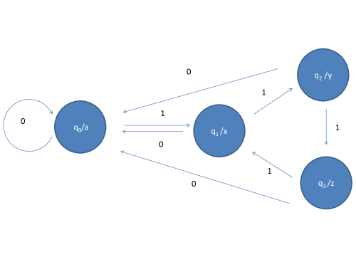
Figure 1. The automaton generating $\eta$

Consider the automaton $\mathcal{A}$ from figure 1. It is an automaton over the alphabet $\{0,1\}$ with four states $q_{0},q_{1},q_{2},q_{3}$, which are labeled by $a,x,y,z$ respectively. Then, the infinite sequence

$$\mathcal{A}_{q_{0}}:\mathbb{N}\cup\{0\}\longrightarrow\{a,x,y,z\}$$

generated by the automaton with initial state $q_{0}$ is defined as follows: Write $n\in\mathbb{N}\cup\{0\}$ in its binary expansion as

$$n=x_{0}2^{i}+x_{1}2^{i-1}+\cdots+x_{i-1}2+x_{i}$$

with $i\in\mathbb{N}\cup\{0\}$ and $x_{j}\in\{0,1\}$, $j=0,\ldots,i$. Consider now the path $p_{n}$ in the automaton starting in $q_{0}$ and following the sequence $x_{0}x_{1}\ldots x_{i}$. Then, $\mathcal{A}_{q_{0}}(n)$ is defined to be the label of the state where this path ends.

Theorem 3.23.

The fixed point $\eta$ of $\tau$ agrees with $\mathcal{A}_{q_{0}}$ (where the fixed point is considered as a map from $\mathbb{N}\cup\{0\}$ to $\{a,x,y,z\}$).

This theorem is an immediate consequence of the next proposition. To state the proposition we will need some further pieces of notation. For each $n\in\mathbb{N}\cup\{0\}$ and each state $q$ of the automaton we define $f^{(n)}(q)$ to be the word over $\{a,x,y,z\}$ of length $2^{n}$ obtained in the following way: Let $v_{1},\ldots,v_{2^{n}}$ be the list of all words of length $n$ over $\{0,1\}$ in lexicographic order (where $0<1$). Consider now for each $k=1,\ldots,2^{n}$ the path in the automaton starting at $q$ and following the word $v_{k}$. Then, the $k$-th letter of $f^{(n)}(q)$ is defined to be the label of the state where this path ends.

Define the letters

$$s_{n}=\tau^{n}(x)=\left\{\begin{array}[]{ccc}x&:&n=3k,k\in\mathbb{N}\cup\{0\}\\ y&:&n=3k+1,k\in\mathbb{N}\cup\{0\}\\ z&:&n=3k+2,k\in\mathbb{N}\cup\{0\}\end{array}\right.$$

and recall the recursion formula

$$p^{(n+1)}=p^{(n)}s_{n}p^{(n)}$$

with $p^{(n)}:=\tau^{n}(a)$.

Proposition 3.24.

For each natural number $n$ and each $i=0,1,2,3$ we have

$$f^{(n+1)}(q_{i})=p^{(n)}s_{n+i}.$$

Proof.

This is proven by induction. The case $n=1$ follows by inspection. Assume now that the statement is true for some $n\geq 1$ and consider $n+1$. Then the lexicographic ordering of the words of length $n+2$ over $\{0,1\}$ is given by

$$0v_{1},\ldots 0v_{2^{n+1}},1v_{1},\ldots 1,v_{2^{n+1}},$$

where $v_{1},\ldots,v_{2^{n+1}}$ is the lexicographic ordering of the words of length $n+1$ over $\{0,1\}$. Thus, from the rules of the automaton we obtain for each $i=0,1,2,3$

$$f^{(n+2)}(q_{i})=f^{(n+1)}(q_{0})f^{(n+1)}(q_{i+1}),$$

where we set $q_{4}=q_{1}$. From our assumption for $n$ and the recursion we then find

$$f^{(n+2)}(q_{i})=p^{(n)}s_{n}p^{(n)}s_{n+1+i}=p^{(n+1)}s_{n+1+i}$$

for each $i=0,1,2,3$ and this is the desired statement. ∎

3.7. Replacing $\tau$ by a primitive substitution

The substitution $\tau$ arises naturally in the study of Grigorchuk groups $G$ and its Schreier graphs (see below). From the point of view of subshifts it has the (slight) disadvantage of not being primitive. It turns out that it is possible to find a primitive substitution $\xi$ with the same fixed point - and hence the same subshift - as $\tau$. This can then be used to obtain alternative proofs for the (proven above) linear repetitivity and pure discreteness of the spectrum. This is discussed at the end of this section. The material presented here was pointed out to us by Fabien Durand [31].

Consider the substitution $\zeta$ on the alphabet $\{a,x,y,z\}$ with

$$\zeta(a)=ax,\zeta(x=ay,\zeta(y)=az,\zeta(z)=ax(=\zeta(a)).$$

As any letter of the alphabet is contained in $\zeta^{4}(s)$ for any letter $s$, this is a primitive substitution.

To relate it to $\tau$ we use (again) for $n\in\mathbb{N}\cup\{0\}$ the letters $s_{n}=\tau^{n}(x)$ as well as the recursion formula $p^{(n+1)}=p^{(n)}s_{n}p^{(n)}$ with $p^{(n)}:=\tau^{n}(a)$.

Proposition 3.25.

For any natural number $n$ the equality

$$\zeta^{n}(a)=\tau^{n-1}(a)s_{n-1}$$

holds. In particular, the fixed point $\eta$ of $\tau$ agrees with the fixed point of $\zeta$.

Proof.

This is shown by induction. The cases $n=1,2,3$ are easily checked by direct inspection. Assume now that the statement is true for all integers up to some $n\geq 3$. Then, we can compute

$$\zeta^{n+1}(a)=\zeta^{n}(ax)=\zeta^{n}(a)\zeta^{n}(x)=\zeta^{n}(a)\zeta^{n-1}(ay)=...=\zeta^{n}(a)\zeta^{n-1}(a)\zeta^{n-2}(a)\zeta^{n-3}(ax).$$

By $\zeta(a)=ax$ we then find

$$\zeta^{n+1}(a)=\zeta^{n}(a)\zeta^{n-1}(a)\zeta^{n-2}(a)\zeta^{n-2}(a).$$

From our assumption on $n$ we then infer

$$\zeta^{n+1}(a)=\tau^{n-1}(a)s_{n-1}\tau^{n-2}(a)s_{n-2}\tau^{n-3}(a)s_{n-3}\tau^{n-3}(a)s_{n-3}.$$

Successive application of the recursion formula and the fact that $s_{n-3}=s_{n}$ then give

$$\zeta^{n+1}(a) = \tau^{n-1}(a)s_{n-1}\tau^{n-2}(a)s_{n-2}(\tau^{n-3}(a)s_{n-3}\tau^{n-3}(a))s_{n-3}$$

$$= \tau^{n-1}(a)s_{n-1}\tau^{n-2}(a)s_{n-2}\tau^{n-2}(a)s_{n-3}$$

$$= \tau^{n-1}(a)s_{n-1}\tau^{n-1}(a)s_{n-3}$$

$$= \tau^{n}(a)s_{n-3}$$

$$= \tau^{n}(a)s_{n}.$$

This is the desired statement. ∎

Corollary 3.26.

The subshift $(\varOmega_{\zeta},T)$ generated by the primitive substitution $\zeta$ agrees with the subshift $(\varOmega_{\tau},T)$.

As it is well known, see e.g. [30, 27], that subshifts associated to primitive substitutions are linearly repetitive, an immediate consequence of the previous corollary is that $(\varOmega_{\tau},T)$ is linearly repetitive. Also, as $\zeta$ has constant length (i.e. the length of $\zeta(t)$ is the same for any letter $t$) and $\zeta(t)$ starts with $a$ for any letter $t$ we can apply a result of Dekking [29] to obtain purely discrete spectrum.

4. Background on graphs and dynamical systems

In this section we recall some basic notions and concepts from the theory of graphs, dynamical systems, and Schreier graphs. In the next section we will meet all these abstract concepts in the context of a particular group.

Here we first recall some terminology from the theory of graphs and introduce the topological space of (isomorphism classes of) rooted labeled graphs.

Let $\mathcal{B}$ be a finite non-empty set together with an involution $\mathcal{B}\longrightarrow\mathcal{B},b\mapsto\overline{b}$. A graph with edges labeled by $\mathcal{B}$ is a pair $(V,E)$ consisting of a set $V$ and a set $E\subset V\times V\times\mathcal{B}$ such that $(v,w,b)$ belongs to $E$ if $(w,v,\overline{b})$ belongs to $E$. The elements of $V$ are called vertices and the elements of $E$ are called edges. Whenever $e=(v,w,b)$ is an edge, then $b$ is called the label, $v=o(e)$ the origin and $w=t(e)$ the terminal vertex of the edge. We say that there is an edge from the vertex $v$ the the vertex $w$ with label $b$ if $(v,w,b)$ belongs to $E$. An edge $e$ is said to emanate from the vertex $v$ if $v=o(e)$. The number of edges emanating from a vertex is called the degree of the vertex. An edge of the form $(v,v,b)$ is called a loop at $v$ (with label $b$).

We will a need the combinatorial distance on a graph given as follows. Each vertex has distance $0$ to itself. The distance between different vertices $v$ and $w$ is one if and only if there exists a label $b$ such that $(v,w,b)$ belongs to $E$. More generally the distance between different vertices $v$ and $w$ is then defined inductively as the smallest natural number $n$ such that there exists a vertex $v^{\prime}$ with distance $n-1$ to $v$ and distance one to $w$. If no such $n$ exists the combinatorial distance is defined to be $\infty$. The graph is called connected if the distance between any two if its vertices is finite. Likewise the connected component of a vertex is the set of all vertices with finite distance to it.

A ray in an infinite graph is an infinite sequence $v_{0},v_{1},\ldots$ of pairwise different vertices with distance one between consecutive vertices. Two rays are equivalent if there exists a third ray containing infinitely many vertices of each of the rays. An equivalence class of rays is called an end of the graph. For example finite graphs have $0$ ends, the Cayley graphs of $\mathbb{Z}$, $\mathbb{Z}^{2}$ and $\mathbb{F}_{2}$ (the free group on two letters) have $2,1$ and infinitely many ends, respectively. In general the Cayley graph of a group may have $0,1,2$ or infinitely many ends.

A rooted graph is a pair consisting of a graph and a vertex belonging to the vertex set of the graph. This vertex is then called the root.

Two rooted graphs $(G_{1},v_{1})$ and $(G_{2},v_{2})$ labeled by the same set $\mathcal{B}$ are called isomorphic if there exists a bijective map $\beta$ from the vertices of $G_{1}$ to the vertices of $G_{2}$ taking $v_{1}$ to $v_{2}$ such that the vertices $x$ and $y$ in $G_{1}$ are connected by an edge of color $b$ if and only if their images in $V(G_{2})$ are connected by an edge of color $b$. In this case we write $(G_{1},v_{1})\cong(G_{2},v_{2})$.

Let us now consider the set $\mathcal{G}_{*}(\mathcal{B})$ of isomorphism classes of connected rooted graphs labeled with elements from $\mathcal{B}$ that we endow with the following natural metric. The distance between the isomorphism classes of the two rooted graphs $(Y_{1},v_{1})$ and $(Y_{2},v_{2})$ is then defined as

$$\mbox{dist}([(Y_{1},v_{1})],[(Y_{2},v_{2})]):=\inf\left\{\frac{1}{r+1}:B_{Y_{1}}(v_{1},r)\cong B_{Y_{2}}(v_{2},r)\right\}$$

where $B_{Y}(v,r)$ is the (labeled) ball of radius $r$ centered in $v$ in the combinatorial metric on $Y$. If we only consider graphs of uniformly bounded degree (as we will in this paper), the space $\mathcal{G}_{*}(\mathcal{B})$ is compact.

We now turn to dynamical systems. Whenever the group $H$ acts on the compact space $Y$ via the continuous map $\alpha:H\times Y\longrightarrow Y$ we call $(Y,H,\alpha)$ a dynamical system. We will mostly suppress the $\alpha$ in the notation. In particular, we will write $(Y,H)$ instead of $(Y,H,\alpha)$ and we will write $ty$ for $\alpha_{t}(y)$ (with $y\in Y$ and $t\in H$). If $H$ is the infinite cyclic group $\mathbb{Z}$, then the action of $H$ on $Y$ is determined by $T:=\alpha(1)$ and we then just write $(Y,T)$ instead of $(Y,\mathbb{Z})$ (and this is well in line with the notation used in the previous sections).

Whenever a dynamical system $(Y,H)$ and $y\in Y$ is given we call

$$\{ty:t\in H\}$$

the orbit of $y$ (under H).

The dynamical system $(Y,H)$ is minimal if every orbit is dense in $Y$. The dynamical system $(Y,H)$ is called uniquely ergodic if there exists exactly one $H$-invariant probability measure on $Y$.

The dynamical system $(Y,H)$ is called a factor of the dynamical system $(Y^{\prime},H)$ if there exist a continuous surjective map $\chi:Y^{\prime}\longrightarrow Y$ with $\chi(ty)=t\chi(y)$ for all $t\in H$ and $y\in Y^{\prime}$. This map $\chi$ is then called factor map. The dynamical system $(Y,H)$ is then also referred to as extension of the dynamical system $(Y^{\prime},H)$.

We will deal with graphs arising from dynamical systems. More specifically, consider a group $H$ generated by a symmetric finite set $S$ and assume that $H$ acts on the compact space $Y$. Then any point $y\in Y$ gives rise to the orbital Schreier graph of $y$ denoted by $\varGamma_{y}$. This is a rooted graph labeled by $S$, which is equipped with the involution $S\longrightarrow S,s\mapsto s^{-1}$. The set of vertices of $\varGamma_{y}$ is given by the points in the orbit of $y$. The root is given by $y$ and rhere is an edge from $v$ to $w$ with label $s\in S$ if $sx=y$. Note that by the required symmetry of $S$ we then have also an edge from $w$ to $v$ with label $s^{-1}$ (as is needed according to our definition of a labeled graph).

As an example we note the Cayley graph of a group $G$ with generating set $S$. This Cayley graph (with the neutral element of $G$ as the root) is the orbital Schreier graph of $G$ corresponding to the action of $G$ on itself via left multiplication.

If the elements of $S$ happen to all be involutions then there will be an edge of label $s$ from $v$ to $w$ if and only if there is an edge of label $s$ from $w$ to $v$. This is the situation we will encounter in the next section.

5. Grigorchuk’s group $G$, its Schreier graphs and the associated Laplacians

In this section we introduce the main object of our interest: the first group of intermediate growth $G$ and the Laplacians on the associated Schreier graphs. The group $G$ is the first group with intermediate word growth and was introduced by the first author in [36, 37]. By now it is generally known as Grigorchuk’s group $G$ and this is how we will refer to it. It is generated by four involutions $a,b,c,d$. With notation to be introduced presently, the group $G$ can be viewed as a group acting by automorphisms on the full infinite binary tree $\mathcal{T}$. The action extends by continuity to an action by homeomorphisms on the boundary $\partial\mathcal{T}$. The action of $G$ gives rise to Schreier graphs

The Schreier graphs arising from actions of automorphism groups of infinite regular rooted trees have attracted substantial attention in recent years [43, 70]. Of particular interest are so-called self-similar groups (as $G$) whose action reflect the self-similar structure of the tree. Their Schreier graphs also have self-similarity features. Some are closely related to Julia sets [11, 28, 70], others are fractal sets close to e.g. the Sierpinski gasket or the Apollonian gasket [10, 44, 45].

The spectra of the Laplacians on such graphs have been described in some cases [10, 44, 45, 42, 46]. The spectrum can be a union of intervals [42], a Cantor set [10], or a union of a Cantor set together with an infinite set of isolated points that accumulate to it, as in the case of the so-called Hanoi tower group [45]. These investigations all use the method introduced in [10]. Here we study the spectra of the Laplacians on the Schreier graphs by a different method via the connection to aperiodic order. This allows us to determine the spectral type of the Laplacians for arbitrary choice of weights on the generators of the group. We thus obtain one of the rare examples where we understand how the spectrum of the Laplacian depends on the weights. In general this dependence is very poorly understood, as well as the dependence of the spectrum on the generating set in the group. Let us mention here a recent result of Grabowski and Virag who show in [35] that there is a weighted Laplacian on the lamplighter group that has singular continous spectrum, whereas the unweighted Laplacian on the same generators is known to have pure point spectrum [46].

5.1. Grigorchuk’s group G

Let us denote by $\mathcal{T}_{q}$, $q\in\mathbb{N}$ with $q\geq 2$, the rooted regular tree of degree $q$. The vertex set of $\mathcal{T}_{q}$ is given by $\{0,\ldots,q-1\}^{\ast}$, i.e. the set of all words over the alphabet $\{0,\ldots,q-1\}$. The root of $\mathcal{T}_{q}$ is the empty word. There is an edge between $v$ and $w$ whenever $w=vk$ or $v=wk$ holds for some $k\in\{0,\ldots q-1\}$. The words $w\in\{0,\ldots,q-1\}^{n}$ constitute the $n$-the level of the tree. (In the tree, they are at combinatorial distance exactly $n$ from the root.)

The boundary $\partial\mathcal{T}_{q}$ of $\mathcal{T}_{q}$ consisting of infinite geodesic rays in $\mathcal{T}_{q}$ emanating from the root (i.e. infinite paths starting in the root all of whose edges are pairwise different) can then be identified with the set $\{0,1,\ldots,q-1\}^{\mathbb{N}}$ of one-sided infinite words over $\{0,1,\ldots,q-1\}$. As mentioned above, the set $\{0,1,\ldots,q-1\}^{\mathbb{N}}$ is equipped with the product topology and is thus a compact space homeomorphic to the Cantor set.

Any automorphism of $\mathcal{T}_{q}$ necessarily preserves the root (which is the only vertex with degree $q$) and maps paths starting in the root to paths starting in the root. This readily implies that any automorphisms group action on $\mathcal{T}_{q}$ is level preserving, i.e. maps words of length $n$ to words of length $n$. Any such action then extends to an action of the same group by homeomorphisms on the boundary $\partial\mathcal{T}_{q}$.

A regular rooted tree is a self-similar object. Indeed, the subtree rooted at an arbitrary vertex of the tree is isomorphic to the whole tree $\mathcal{T}_{q}$. The full group of automorphisms inherits this self-similarity property in the following sense: any automorphism of $\mathcal{T}_{q}$ is completely determined by the permutation it induces on the $q$ branches growing from the root (an element of $Sym(q)$) and the collection of $q$ automorphisms $(g_{0},...,g_{q-1})$ which coincide with the restrictions of $g$ on the corresponding branches.

However, if one is interested in a subgroup $H<Aug(T_{q})$ and wants it to be self-similar, one has to impose the condition that all the restrictions $(g_{0},...,g_{q-1})$ are again elements of the same group $H$, so that every $g\in H$ can be represented as

$$g=\alpha(g_{0},\ldots,g_{q-1}),$$

where $\alpha$ belongs to $\mbox{Sym}(q)$ and describes the action of $g$ on the first level of $\mathcal{T}_{q}$ and $g_{i}\in G,i=0,...,q-1$ is the restriction of $g$ on the full subtree of $\mathcal{T}_{q}$ rooted at the vertex $i$ of the first level of $\mathcal{T}_{q}$. This leads to the following definition.

Definition 5.1.

A group $H$ of automorphisms of $\mathcal{T}_{q}$ is self-similar if, for all $g\in H,x\in\{0,\ldots,q-1\}$, there exist $h\in H,y\in\{0,\ldots,q-1\}$ such that

$$g(xw)=yh(w),$$

for all finite words $w$ over the alphabet $\{0,\ldots,q-1\}$.

We refer the interested reader to [43, 70] for more information about self-similar groups.

We now turn our attention to one particular example of a self-similar group that will be the central object of our study, the Grigorchuk group $G$. It is generated by four automorphisms $a,b,c,d$ of the rooted binary tree $\mathcal{T}=\mathcal{T}_{2}$ as follows:

• $a(0w)=1w$, $a(1w)=0w;$

• $b(0w)=0a(w)$, $b(1w)=1c(w);$

• $c(0w)=0a(w)$, $c(1w)=1d(w);$

• $d(0w)=0w$, $d(1w)=1b(w),$

for an arbitrary word $w$ over $\{0,1\}$. These automorphisms can also be expressed in the self-similar form, as above:

$$a=\epsilon(id,id),\qquad b=e(a,c),\qquad c=e(a,d),\qquad d=e(id,b),$$

where $e$ and $\epsilon$ are, respectively, the trivial and the non-trivial permutations in the group $\mbox{Sym}(2)$.

Remark 5.2.

Observe that all the generators are involutions and that $\{1,b,c,d\}$ commute and constitute a group isomorphic to the Klein group $\mathbb{Z}/2\mathbb{Z}\times\mathbb{Z}/2\mathbb{Z}$. Let as also mention that there are many more relations and the group is not finitely presented.

For our subsequent discussion it will be important that $G$ acts transitively on each level, i.e. for arbitrary words $w,u$ over $\{0,1\}$ with the same length there exists a $g\in G$ with $gu=w$.

5.2. The Schreier graphs of $G$ and the dynamical system $(X,G)$

The action of $G$ on the set $V\{0,1\}^{\ast}$ of vertices of the rooted binary tree and on its boundary $\partial\mathcal{T}=\{0,1\}^{\mathbb{N}}$ induces on this set the structure of a graph labeled with $\{a,b,c,d\}\subset G$. Specifically, the vertex set of this graph is given by $\{0,1\}^{\ast}\cup\{0,1\}^{\mathbb{N}}$ and there is an edge with label $s\in\{a,b,c,d\}$ and origin $v$ and terminal vertex $w$ if and only if $sv=w$ holds. Note that the set of arising edges has indeed the symmetry property required in our definition of a labeled graph as any $s\in\{a,b,c,d\}$ is an involution. For the first three levels of the tree the resulting graphs are shown in Figure 2. The connected components of this graph correspond to the orbits of the group action. Thus, the rooted graphs consisting of such a connected component together with a root are orbital Schreier graphs (in the sense defined above).

There are two kind of such connected components viz finite and infinite components. The finite ones correspond to the levels of the tree (recall that the action of $G$ on the levels of the tree is transitive). We will refer to them simply as Schreier graphs. The infinite ones correspond to the orbits of the action on the boundary. The corresponding rooted graphs will be referred to as orbital Schreier graphs.

Figure 2. The finite Schreier graphs of the first, second and third level.

We will need the isomorphism classes of Schreier graphs and introduce therefore the map

$$\mathcal{F}:V(\mathcal{T})\cup\partial\mathcal{T}\longrightarrow\mathcal{G}_{*}(\{a,b,c,d\}),\;\mathcal{F}(v):=[(\varGamma_{v},v)],$$

where $\varGamma_{v}$ is the connected component of $v$.

The graphs $\varGamma_{w}$ and $\varGamma_{v}$ coincide (as non-rooted graphs) whenever $v$ and $w$ are in the same orbit of the action of $G$. In particular, as $G$ acts transitively on each level of the tree, for $n\in\mathbb{N}$ we can therefore define

$$\varGamma_{n}:=\varGamma_{1^{n}}$$

which coincides with $\varGamma_{w}$ for all $w\in V(\mathcal{T})$ with $|w|=n$. In general, the graph $\Gamma_{n}$ has a linear shape; it has $2^{n-1}$ simple edges, all labeled by $a$, and $2^{n-1}-1$ cycles of length 2 whose edges are labeled by $b,c,d$. It is regular of degree 4, with one loop at each edge. The loop contributes 1 to the degree of the vertex because all generators are elements of order 2, and the labeling of the loop is uniquely determined by the labeling of the other edges around the vertex, as edges around one vertex are labeled by $\{a,b,c,d\}$.

The graphs $\varGamma_{\xi}$, $\xi\in\partial\mathcal{T}$ corresponding to the action of $G$ on the boundary are infinite and have either two ends or one end. The graph $\Gamma_{1^{\infty}}$ corresponding to the orbit of the rightmost infinite ray, is one-ended (see Figure 3), and so are then all graphs in the same orbit.

Figure 3. The one-ended graph $\varGamma_{1^{\infty}}$.

All the other graphs $\Gamma_{\xi},\xi\notin G\cdot 1^{\infty}$, are two-ended. They are all isomorphic as unlabeled graphs.

In [80], Vorobets studied the closure $\overline{\mathcal{F}(\partial\mathcal{T})}$ of the space of Schreier graphs in the space of isomorphism classes of rooted labeled graphs. We recall some of his results next. He showed that the one-ended graphs are exactly the isolated points of this closure $\overline{\mathcal{F}(\partial\mathcal{T})}$, and that the other points in $\overline{\mathcal{F}(\partial\mathcal{T})}$ are two ended graphs. This suggests to consider the compact set

$$X:=\overline{\mathcal{F}(\partial\mathcal{T})}\setminus\{\text{isolated points}\}.$$

The group $G$ acts on $X$ by changing the root of the graph. The arising dynamical system is denoted as $(X,G)$. It is minimal and uniquely ergodic and its invariant probability measure will be denoted as $\nu$.

A precise description of $X$ can be given as follows. The space $X$ consists of all isomorphism classes of two-ended rooted Schreier graphs $\{(\Gamma_{\xi},\xi):\xi\in\partial\mathcal{T}\setminus G\cdot 1^{\infty}\}$ and of three additional countable families of isomorphism classes of two-ended graphs. These families are obtained by gluing two copies of the one-ended graph $\Gamma_{\xi},\xi\in G\cdot 1^{\infty}$, at the root in three possible ways corresponding to choosing a pair $(b,c)$, $(b,d)$ or $(c,d)$ and then choosing an arbitrary vertex of the arising graph as the root. One of these three possibilities is shown in Figure 4. There, the chosen pair is $(c,d)$ and to avoid confusion with other edges with the same labels, labels at the gluing point are denoted with a prime.

Figure 4. Connecting two copies of $\Gamma_{1^{\infty}}$

The decomposition of $X$ into isomorphism classes of the $(\varGamma_{\xi},\xi)$ and the three families mentioned above gives immediately rise to a factor map

$$\phi:X\rightarrow\partial\mathcal{T},$$

which is one-to-one except in a countable set of points, where it is three-to-one. In fact, the inverse map $\phi^{-1}$ exists on the complement $\partial\mathcal{T}\setminus G\cdot 1^{\infty}$ of the orbit of the point $1^{\infty}$ and agrees there with $\mathcal{F}$.

Under this factor map $\phi$ the unique $G$-invariant probability measure $\nu$ on $X$ is mapped to the uniform Bernoulli measure $\mu$ on $\partial\mathcal{T}=\{0,1\}^{\mathbb{N}}$.

5.3. Laplacians associated to the Schreier graphs of $G$

Whenever a group $H$ acts on a measure space $(Y,m)$ by measure preserving transformations, one obtains the Koopman representation $\varrho$ of $H$ on $L^{2}(Y,m)$ via

$$\varrho(h):L^{2}(Y,m)\longrightarrow L^{2}(Y,m),(\varrho(h)f)(y)=f(h^{-1}y),$$

(for $h\in H$). Any $\varrho(h)$ is then a unitary operator (as the action is measure preserving).

In our situation when $H=G$, we have moreover that for $s\in\{a,b,c,d\}$ the unitary operator $\varrho(s)$ is its own inverse (as $s$ is an involution) and hence must be selfadjoint. In particular, for any set of parameters $t,u,v,w\in\mathbb{R}$ we obtain a selfadjoint operator

$$M_{\varrho}(t,u,v,w):=t\varrho(a)+u\varrho(b)+v\varrho(c)+w\varrho(d).$$

Consider first an arbitrary $\xi\in\partial\mathcal{T}$. Then, there is an action of $G$ on the (countable) vertex set of $V(\varGamma_{\xi})$ of $\varGamma_{\xi}$. Specifically, $s\in\{a,b,c,d\}$ maps the vertex $x\in V(\varGamma_{\xi})$ to the vertex $sx$, which is the unique vertex of $V(\varGamma_{\xi})$ connected to $v$ by an edge of label $s$. Clearly, this action preserves the counting measure on $V(\varGamma_{\xi})$. Thus, we obtain a representation $\varrho_{\xi}$ of $G$ on $\ell^{2}(V(\varGamma_{\xi}))$.

Definition 5.3 (Laplacian of the Schreier graph).

An operator $M_{\xi}(t,u,v,w)$ defined by

$$M_{\xi}(t,u,v,w):=M_{\varrho_{\xi}}(t,u,v,w)=t\varrho_{\xi}(a)+u\varrho_{\xi}(b)+v\varrho_{\xi}(c)+w\varrho_{\xi}(d)$$

with $\xi\in\partial\mathcal{T}$ and $t,u,v,w\in\mathbb{R}$ will be called (weighted) Laplacian of the Schreier graph $\varGamma_{\xi}$.

Remark 5.4.

• It is possible to understand $V(\varGamma_{\xi})$ as $G/G_{\xi}$, where $G_{\xi}$ is the stabilizer of $\xi$ in the action of $G$ on $\partial\mathcal{T}$, and then $\varrho_{\xi}$ is the quasi-regular representation $\varrho_{G/G_{\xi}}$ associated to $G/G_{\xi}$.

• If $t,u,v,w$ are positive with $1=t+u+v+w$ then it is possible to interpret the operators $M_{\xi}$ as the Markov operators of a random walk on the graph $\varGamma_{\xi}$. In the general case, the operator $M_{\xi}(t,u,v,w)$ can still be seen as the natural weighted ’adjacency matrix’ or ’Laplacian’ associated to the the graph $\varGamma_{\xi}$.

We can also equip $\partial\mathcal{T}=\{0,1\}^{\mathbb{N}}$ with the uniform Bernoulli measure $\mu$ and consider the Koopman representation $\pi$ of $G$ on $L^{2}(\partial\mathcal{T},\mu)$ given via

$$\pi(g):L^{2}(\partial\mathcal{T},\mu)\longrightarrow L^{2}(\partial\mathcal{T},\mu),\pi(g)f(x)=f(g^{-1}x).$$

This is a unitary representation of $G$ and any $\pi(s)$, $s\in\{a,b,c,c\}$, is a unitary selfadjoint involution. For $t,u,v,w\in\mathbb{R}$ we then obtain the operator $M_{\pi}(t,u,v,w)$ via

$$M_{\pi}(t,u,v,w)=t\pi(a)+u\pi(b)+v\pi(c)+w\pi(d).$$

The following is a crucial result on the spectral theory of the above operators.

Theorem 5.5 (Independence of spectrum (Bartholdi / Grigorchuk [10])).

For any given set of parameters $t,u,v,w\in\mathbb{R}$ the spectrum of $M_{\xi}(t,u,v,w)$ does not depend on $\xi\in\partial\mathcal{T}$ and coincides with the spectrum of $M_{\pi}(t,u,v,w)$.

Of course, there is the question what the spectrum is in terms of the parameters $t,u,v,w$. A complete answer was given in [10] in the case $u=v=w$. The spectrum then consists of two points or one or two intervals, and an explicit description of the spectrum can be given in terms of the parameters$t$ and $u=v=w$. In fact, the case $u=v=w$ is the case of periodic Schrödinger type operators and can easily be treated by classical means (Floquet decomposition). It can also be treated by the method suggested in [10]. For related results on the Kesten-von-Neummann-Serre trace we refer to [39]. Below we will come to a main result of [40] which treats the case, where $u=v=w$ does not hold. We will see that in this case, the spectrum is a Cantor set of Lebesgue measure zero.

6. The connection between $(X,G)$ and $(\varOmega_{\tau},T)$

We will now provide a map gr from $\varOmega_{\tau}$ to (isomorphism classes of) labeled rooted graphs with labels belonging to the alphabet $\{a,b,c,d\}$. In order to get a better understanding of this map it will be useful to think of the letters $x,y,z$ as encoding the pairs

$$\left(\begin{matrix}b\\ c\end{matrix}\right);\ \ \left(\begin{matrix}b\\ d\end{matrix}\right);\ \left(\begin{matrix}c\\ d\end{matrix}\right)$$

respectively. Roughly speaking the map will convert $\omega\in\varOmega_{\tau}$ into a graph with vertex set $\mathbb{Z}$ and root $1$ and edges between $n$ and $n+1$ with labels from $\{a,b,c,d\}$ according to the value of $\omega(n)$. We now provide the precise definition of the labeled rooted graph $\mbox{gr}(\omega)$ associated to $\omega\in\varOmega_{\tau}$ as follows:

Vertices: The set of vertices is $\mathbb{Z}$.

Root: The number $1$ is chosen as the root.

Edges: There are edges between vertices $n,k$ if an only if $|n-k|\leq 1$. Specifically, edges are assigned between $n$ and $n+1$ and from $n$ to itself and from $n+1$ to itself in the following way:

• If $\omega(n)=a$, then there is an edge between $n$ and $n+1$ and this edge carries the label $a$.

• If $\omega(n)=x$, then there are two edges between $n$ and $n+1$; one carries the label $b$ and the other carries the label $c$. Moreover, there is an additional edge from $n$ to itself labeled with $d$ and an additional edge from $n+1$ to itself labeled with $d$.

• If $\omega(n)=y$, then there are two edges between $n$ and $n+1$; one carries the label $b$ and the other carries the label $d$. Moreover, there is an additional edge from $n$ to itself labeled with $c$ and an additional edge from $n+1$ to itself labeled with $c$.

• If $\omega(n)=z$, then there are two edges between $n$ and $n+1$; one carries the label $c$ and the other carries the label $d$. Moreover, there is an additional edge from $n$ to itself labeled with $b$ and an additional edge from $n+1$ to itself labeled with $b$.

We note that in this way any vertex has for each label $\{a,b,c,d\}$ exactly one edge of this color emanating from it. We also note that the arising graphs have a ’linear structure’ in a natural sense.

Let $\mathcal{G}_{*}(\{a,b,c,d\})$ be the metric space of isomorphism classes of connected rooted graphs labeled with elements from $\{a,b,c,d\}$. Then, gr gives rise to a map Gr via

$$\mbox{Gr}:\varOmega_{\tau}\longrightarrow\mathcal{G}_{*}(\{a,b,c,d\}),\omega\mapsto[\mbox{gr}(\omega)],$$

where $[(\varGamma,v)]$ is the equivalence class of $(\varGamma,v)$ in the space of isomorphism classes of the rooted connected labeled graphs.

Recall that $X$ denotes the closure of $\mathcal{F}(\mathcal{T})$ in $\mathcal{G}_{*}(\{a,b,c,d\})$ without its isolated points (see Section 5.2). Then, it turns out that the image of $\varOmega_{\tau}$ under Gr is exactly $X$. In fact, much more is true and this is our main result on the connection of the subshift $(\varOmega_{\tau},T)$ and the dynamical system $(X,G)$.

Define the maps $A,B,C,D$ from $\varOmega_{\tau}$ into itself by

• $A(\omega)=...\omega_{0}\omega_{1}|\omega_{2}...$ if $\omega_{1}=a$ and $A(\omega)=....\omega_{-1}|\omega_{0}\omega_{1}...$ if $\omega_{0}=a$.

• $B(\omega)=...\omega_{0}\omega_{1}|\omega_{2}...$ if $\omega_{1}\in\{x,y\}$, $B(\omega)=....\omega_{-1}|\omega_{0}\omega_{1}...$ if $\omega_{0}\in\{x,y\}$ and $B(\omega)=\omega$ in all other cases.

• $C(\omega)=...\omega_{0}\omega_{1}|\omega_{2}...$ if $\omega_{1}\in\{x,z\}$, $C(\omega)=....\omega_{-1}|\omega_{0}\omega_{1}...$ if $\omega_{0}\in\{x,z\}$ and $C(\omega)=\omega$ in all other cases.

• $D(\omega)=...\omega_{0}\omega_{1}|\omega_{2}...$ if $\omega_{1}\in\{y,z\}$, $D(\omega)=....\omega_{-1}|\omega_{0}\omega_{1}...$ if $\omega_{0}\in\{y,z\}$ and $D(\omega)=\omega$ in all other cases.

Then, clearly, $A,B,C,D$ are homeomorphisms and involutions. Let $H$ be the group generated by $A,B,C,D$ (within the group of homeomorphisms of $\varOmega_{\tau}$).

Theorem 6.1 (Factor theorem [40]).

The following statements hold:

(a) The group $G$ is isomorphic to the group $H$ via $\varrho:G\longrightarrow H$ with $\varrho(a)=A$, $\varrho(b)=B$, $\varrho(c)=C$ and $\varrho(d)=D$. In particular, there is a well defined action $\alpha$ of $G$ on $\varOmega_{\tau}$ given by $\alpha_{g}(\omega):=\varrho(g)(\omega)$ for $g\in G$ and $\omega\in\varOmega_{\tau}$ and via this action we obtain a dynamical system $(\varOmega_{\tau},G)$.

(b) The dynamical system $(X,G)$ is a factor of the dynamical system $(\varOmega_{\tau},G)$ with factor map

$$\psi:\varOmega_{\tau}\longrightarrow X,\omega\mapsto\mbox{Gr}(\omega),$$

which is two-to-one.

(c) For every $\omega\in\varOmega_{\tau}$ the orbits $\{T^{n}\omega:n\in\mathbb{Z}\}$ and $\{\alpha_{g}(\omega):g\in G\}$ coincide.

(d) The dynamical system $(\varOmega_{\tau},G)$ is uniquely ergodic and the unique $T$-invariant probability measure on $\varOmega_{\tau}$ coincides with the unique $G$-invariant probability measure on $\varOmega_{\tau}$.

The theorem provides a factor map $\psi:(\varOmega_{\tau},G)\longrightarrow(X,G)$. In Section 5.2 we have already encountered the factor map $\phi:(X,G)\longrightarrow(\partial\mathcal{T},G)$. Putting together these factor maps provide a tower of extensions of the dynamical system $(\partial\mathcal{T},G)$ via

$$(\varOmega_{\tau},G)\stackrel{{\scriptstyle\psi}}{{\longrightarrow}}(X,G)\stackrel{{\scriptstyle\phi}}{{\longrightarrow}}(\partial\mathcal{T},G).$$

The remainder of this section is devoted to providing additional perspective on these two factor maps by discussing their respective merits. We will see that $\phi$ resolves the non-typical points and that $\psi$ allows one to embed the group $G$ into a topological full group.

We will need a bit of notation first. Let $(Y,H)$ be a dynamical system. Let $g\in H$ be given. Then, an $y\in Y$ is called $g$-typical if either $gy\neq y$ or $g$ acts trivially in some neighborhood of $y$. If $y\in Y$ is $g$-typical for any $g\in H$ it is called typical. Typical points have many claims to be indeed typical. For instance, if $H$ is countable the set of typical points has a meager complement [38]. Moreover, the following is shown in [43, 38].

Proposition 6.2.

Let $(Y,H)$ be a minimal dynamical system and $H$ finitely generated. Then, the Schreier graphs of typical points are locally isomorphic (as labeled graphs). Moreover, if $x\in Y$ is typical and $y\in Y$ is not typical, then any ball around a vertex of $\varGamma_{x}$ is isomorphic to a ball around some vertex in $\varGamma_{y}$.

In order to get a further understanding of the typical points we will next discuss another characterization of typical points. Define the stabilizer of $y$ as

$$\mbox{st}_{H}(y):=\{h\in H:hy=y\}.$$

and the neighborhood stabilizer of $y$ as

$$\mbox{st}_{H}^{0}:=\{g\in H:\mbox{ $h$ acts as identity on a neighborhood of $y$}\}.$$

Then, $\mbox{st}_{H}^{0}$ is a normal subgroup of $\mbox{st}_{H}$ and the quotient

$$\mbox{germ}(y):=\mbox{st}_{H}(y)/\mbox{st}_{H}^{0}$$

is called the group of germs (at $y$).

Lemma 6.3.

Let $(Y,H)$ be a dynamical system. Then, the following assertions are equivalent for $y\in Y$.

• The point $y$ is typical.

• The group of germs $\mbox{germ}(y)$ is trivial.

Proof.

(i)$\Longrightarrow$ (ii): If $\mbox{germ}(y)$ is not trivial, there exits a $g\in\mbox{st}_{H}\setminus\mbox{st}_{H}^{0}$. Hence, $y$ is not typical.

(ii)$\Longrightarrow$ (i): If $y$ is not typical then there exists a $g\in G$ with $gy=y$ but $g$ is not the identity on a neighborhood of $y$. Thus, $\mbox{germ}(y)$ is not trivial (as it contains the class of $g$). ∎

Remark 6.4.

The points $y$ with non - trivial $\mbox{germ}(y)$ are sometimes called singular.

We will also need the concept, going back to [34], of the (topological) full group $[[T]]$ of a homeomorphism $T:Y\longrightarrow Y$ of the Cantor set $Y$. This is the group of those homeomorphisms of $Y$ that at any point coincide locally with powers of T. It is a countable group with remarkable properties. For example it is amenable if $T$ is minimal [52], its commutator subgroup is simple [68] and it is finitely generated if and only if $T$ is a minimal subshift over a finite alphabet [68].

After these preparations we can now came back to the situation at hand.

The dynamical system $(\partial\mathcal{T},G)$ is minimal and uniquely ergodic. However, it does have non-typical points. In fact, a point in $\partial\mathcal{T}$ is non-typical if and only if it belongs to $G\cdot 1^{\infty}$ (see [80]).

The dynamical system $(X,G)$ is minimal and uniquely ergodic (as discussed in [79]). Moreover, all its points are typical (as can easily be seen). Thus, from this point of view a key merit of $(X,G)$ is to provide an extension of of $(\partial\mathcal{T},G)$ which resolves the non-typical points.

The dynamical system $(\varOmega_{\tau},G)$ is minimal and uniquely ergodic and all its points are typical (as can easily be seen). Moreover, as shown in the previous theorem, the dynamical system $(\varOmega_{\tau},G)$ has the additional feature that there exists a homeomorphism $T$ on $\varOmega_{\tau}$ such that the orbits of $T$ agree with the orbits of $G$. This in turn can be seen to imply that $G$ is a subgroup of the topological full group $[[T]]$ of $T$. In fact, $G$ embeds into the topological full group of $(\Omega_{\tau},T)$, as the action of generators $a,b,c,d$ on $\Omega_{\tau}$ can be represented locally as the action by $T^{\pm 1}$ and $T^{0}=id$, so $G$ embeds into $[[T]]$.

Remark 6.5.

In this context we also mention a recent article of Matte Bon [67] showing that the group $G$ (and other groups of intermediate growth introduced by the first author in [36]) embed into the topological full group $[[\phi]]$ of a minimal subshift $\phi$ over a finite alphabet. While his approach is different from ours it leads to the the same subshift for the group $G$.

We finish this section with the question whether there exists a minimal homeomorphism $S$ on $X$ such that $G$ is a subgroup of $[[S]]$.

7. Spectral theory of the $M_{\xi}$ for $\xi\in\partial\mathcal{T}$

In this section we discuss spectral theory of the operators $M_{\xi}(t,u,v,w)$ (defined in Section 5.3) for arbitrary values of the parameters $t,u,v,w$. We do so by using the results of the previous section to transfer the problem of spectral theory of the operators $M_{\xi}(t,u,v,w)$, $\xi\in\partial\mathcal{T}$, to the field of the spectral theory of discrete Schrödinger operators with aperiodic order, $(H_{\omega})_{\omega\in\varOmega_{\tau}}$.

We consider the subshift $(\varOmega_{\tau},T)$. In order to define the Schrödinger operators we will define specific functions $f,g$ on $\varOmega_{\tau}$ depending on four real parameters $t,u,v,w$. Given these parameters we set

$$D:=u+v+w$$

and define

$$f:\varOmega_{\tau}\longrightarrow\mathbb{R}\;\mbox{by}\;\>f(\omega):=\left\{\begin{array}[]{ccc}t&:&\omega_{0}=a\\ D-w&:&\omega_{0}=x\\ D-v&:&\omega_{0}=y\\ D-u&:&\omega_{0}=z\end{array}\right.$$

and

$$g:\varOmega_{\tau}\longrightarrow\mathbb{R}\;\>\mbox{by}\;\>g(\omega):=\left\{\begin{array}[]{c}w:\omega_{0}\omega_{1}\in\{ax,xa\}\\ v:\omega_{0}\omega_{1}\in\{ay,ya\}\\ u:\omega_{0}\omega_{1}\in\{az,za\}\end{array}\right..$$

For a given $(t,u,v,w)\in\mathbb{R}^{4}$ and these $f,g$ we let $H_{\omega}$, $\omega\in\varOmega_{\tau}$, be the associated operators.

Proposition 7.1.

[40] Let $(t,u,v,w)\in\mathbb{R}^{4}$ be given. Let $\xi\in\partial\mathcal{T}\setminus G\cdot 1^{\infty}$ be arbitrary. Then, there exists an $\omega$ in $\varOmega_{\tau}$ such that $H_{\omega}$ is unitarily equivalent to $M_{\xi}(t,u,v,w)$.

As a consequence of the previous proposition we can translate results on the spectral theory of Schrödinger operators associated to $(\varOmega_{\tau},T)$ into results on the $M_{\xi}$. Recall that the spectrum of the $M_{\xi}(t,u,v,w)$ does not depend on $\xi\in\partial\mathcal{T}$ (due to Theorem 5.5). Define

$$\mathcal{P}:=\{(t,u,v,w)\in\mathbb{R}^{4}:t\neq 0,u+v\neq 0,u+w\neq 0,v+w\neq 0\}.$$

Theorem 7.2 (Intervals vs Cantor spectrum for the $M_{\xi}$ [40]).

Let $(t,u,v,w)\in\mathcal{P}$ be given and let $\Sigma=\Sigma(t,u,v,w)$ be the spectrum of the associated family of Laplacians $M_{\xi}(t,u,v,w)$, $\xi\in\partial\mathcal{T}\setminus G\cdot 1^{\infty}$. Then, the following holds:

(a) If $u=v=w$ holds then $\Sigma$ consists of one or two closed non-trivial intervals and all spectral measures are absolutely continuous.

(b) If $u=v=w$ does not hold then $\Sigma$ is a Cantor set of Lebesgue measure zero and no spectral measure is absolutely continuous.

Proof.

Note that $(\varOmega_{\tau},T)$ is linearly repetitive due to Theorem 3.1. Now, the theorem is a direct consequence of the preceding proposition and Theorem 2.7 and Theorem 2.9. ∎

Remark 7.3.

The case $u=v=w$ has already be treated in [10] and an explicit description of the spectrum (in terms of the value of $u$) has been given there.

We can also use the above considerations to translate results on absence of eigenvalues from the $(H_{\omega})$ to the $M_{\xi}$. Recall that $\mu$ denotes the uniform Bernoulli measure on $\partial\mathcal{T}=\{0,1\}^{\mathbb{N}}$.

Theorem 7.4 (Absence of eigenvalues [40]).

Let $(t,u,v,w)\in\mathcal{P}$ be given and assume that $u=v=w$ does not hold.

(a) For $\mu$-almost every $\xi\in\partial\mathcal{T}$ the operator $M_{\xi}$ does not have eigenvalues.

(b) For any $x\in\phi^{-1}(G1^{\infty})$ the operator $M_{x}$ does not have eigenvalues.

Remark 7.5.

The considerations of this section are concerned with the case $(t,u,v,w)\in\mathcal{P}$. For $(t,u,v,w)\notin\mathcal{P}$ the operators in question can be decomposed as a sum of finitely many different finite dimensional operators each appearing with infinite multiplicity. Thus, the spectrum is pure point with finitely many eigenvalues each with infinite multiplicity.

8. Integrated density of states and Kesten-von-Neumann-Serre spectral measure

In this section we show that the Kesten-von-Neumann-Serre spectral measure actually agrees with the integrated density of states. This result is folklore and certainly known to experts. Also, a recent discussion of a somewhat more general setting can also be found in [1]. Here, we give a direct reasoning for the case at hand based on our approach.

There is one more representation studied in the context of spectral approximation. This representation comes from the action of $G$ on the $n$-th level of the tree. This action clearly preserves the counting measure on the finite set of vertices of the $n$-th level. It hence gives rise to a representation $\varrho_{n}$ of $G$ on the finite dimensional $\ell^{2}(V(\varGamma_{n}))$. For $t,u,v,w\in\mathbb{R}$ we then set

$$M_{n}(t,u,v,w):=M_{\varrho_{n}}(t,u,v,w)=t\varrho_{n}(a)+u\varrho_{n}(b)+v\varrho_{n}(c)+w\varrho_{n}(d).$$

To each such $M_{n}(t,u,v,w)$ we associate the spectral distribution which is the measure $\mu_{n}(t,u,v,w)$ on $\mathbb{R}$ given by

$$\mu_{n}(t,u,v,w):=\frac{1}{|V(\varGamma_{n})|}\sum_{E}\delta_{E},$$

where the sum runs over eigenvalues $E$ of $M_{n}(t,u,v,w)$ counted with multiplicities. In the case $u=v=w$ it is shown in [47] that the measures $\mu_{n}$, $n\in\mathbb{N}$, converge weakly and the limiting measure

$$\mu_{\infty}(t,u,v,w)=\lim_{n\to\infty}\mu_{n}(t,u,v,w)$$

is called the Kesten-von-Neumann-Serre spectral measure there. Next we will show that the limiting measure exists for any values of the parameters $t,u,v,w$ and coincides with the so-called integrated density of states of the associated Schrödinger operators.

For given $(t,u,v,w)\in\mathbb{R}^{4}$ we chose the functions $f,g$ as in the previous sections and let $H_{\omega}$, $\omega\in\varOmega_{\tau}$, be the associated Schrödinger operators.

Theorem 8.1.

Let $(t,u,v,w)\in\mathbb{R}^{4}$ be given. For $n\in\mathbb{N}$, let $M_{n}(t,u,v,w)$ be the corresponding operator on $\varGamma_{n}$ and $\mu_{n}$ its spectral distribution. Then, the sequence of measures $(\mu_{n}(t,u,v,w))_{n}$ converges weakly towards the integrated density of states $k$ of $(H_{\omega})$. In particular, the integrated density of states of the $(H_{\omega})$ agrees with the Kesten-von-Neumann-Serre spectral measure.

Proof.

The graph arising from restricting $\mbox{gr}(\omega^{(x)})$ to the vertex set $[1,|\tau^{n}(a)|]$ and the graph $\varGamma_{n}$ differ at most in $6$ loops at the ends (as is clear from the definitions). Thus, a simple variant of the argument in Proposition 7.1 shows that the restriction of the operator $H_{\omega^{(x)}}$ to $[1,|\tau^{n}(a)|]$ is a perturbation of $M_{n}(t,u,v,w)$ of rank at most $6$. Now, Corollary 2.5 gives the convergence of the $\mu_{n}(t,u,v,w)$ towards the integrated density of states of $(H_{\omega})$. ∎

A few comments on this result are in order. They are gathered in the next remark.

Remark 8.2.

• Denote the $\xi$-independent spectrum of the operators $M_{\xi}(t,u,v,w)$ by $\Sigma(t,u,v,w)$ and the spectrum of $M_{n}(t,u,v,w)$ by $\Sigma_{n}(t,u,v,w)$. Clearly, the support of $\mu_{n}$ is given by $\Sigma_{n}(t,u,v,w)$. By Theorem 2.2 support of the integrated density of states $k$ is given by $\Sigma(t,u,v,w)$. Thus, the previous theorem gives in a certain and very weak sense the convergence of the $\Sigma_{n}(t,u,v,w)$ towards $\Sigma(t,u,v,w)$. In particular, there is an inclusion of spectra as shown in Corollary 2.6.

  In the case at hand, however, convergence of the $\Sigma_{n}(t,u,v,w)$ towards $\Sigma(t,u,v,w)$ holds in a much stronger sense. More precisely, the results of [10] give the following:

  • $\Sigma_{n}(t,u,v,w)\subset\Sigma_{n+1}(t,u,v,w)$ for all $n\in\mathbb{N}$.

  • $\Sigma(t,u,v,w)=\overline{\cup_{n}\Sigma_{n}(t,u,v,w)}$.

  These are rather remarkable features and not at all true for approximation of the integrated density of states of Schrödinger operators in other cases.

  Let us note, however, that there are recent results on approximation of spectra of minimal subshifts with respect to the hausdorff distance by suitable periodic approximations [13].

• It is also worth pointing out that the approximation of the spectra is done ’from below’ i.e. via unions. This is in contrast to other approximation schemes used in the investigations of Schrödinger operators, where the approximation is done ’from above’ i.e. via intersections.

• The feature presented in the preceding two points also explain that the spectrum of $M_{\pi}(t,u,v,w)$ agrees with $\Sigma(t,u,v,w)$. The reason is simply that the representation $\pi$ decomposes as a sum of the representations $\pi_{n}$ (as shown in [10]). Accordingly, $M_{\pi}(t,u,v,w)$ is a sum of the finite dimensional operators $M_{n}(t,u,v,w)$, $n\in\mathbb{N}$, and its spectrum is then given as the closure of the union of the spectra of the $M_{n}(t,u,v,w)$.

References

- [1] M. Abert, B. Virag, A. Thom: Benjamini-Schramm convergence and pointwise convergence of the spectral measure , Preprint 2013.
- [2] J.-P. Allouche, J. Shallit, Automatic Sequences: Theory, Applications, Generalization, Cambridge University Press, Cambridge (2003).
- [3] J. Auslander: Minimal Flows and their Extensions, North-Holland Mathematical Studies 153, Elsevier 1988.
- [4] J.-B. Aujogue, M. Barge, J. Kellendonk, D. Lenz: Equicontinuous factors, proximality and Ellis semigroup for Delone sets, to appear in [53].
- [5] M. Baake, U. Grimm: Aperiodic Order: Volume 1, A Mathematical Invitation, Encyclopedia of Mathematics and its Applications 149, Cambridge university press, Cambridge (2014).
- [6] M. Baake, D. Lenz and R.V. Moody: A characterization of model sets by dynamical systems, Ergodic Theory Dynam. Systems 27 (2007), 341–382.
- [7] M. Baake and D. Lenz: Dynamical systems on translation bounded measures: Pure point dynamical and diffraction spectra, Ergod. Th. & Dynam. Systems 24 (2004) 1867–1893.
- [8] M. Baake, R. Moody (Eds.): Directions in Mathematical Quasicrystals, CRM Monogr. Ser. 13, Amer. Math. Soc., Providence, RI (2000).
- [9] M. Barge, J. Kellendonk: Proximality and pure point spectrum for tiling dynamical systems, to appear in: Michigan Journal of Mathematics.
- [10] L. Bartholdi and R. I. Grigorchuk: On the spectrum of Hecke type operators related to some fractal groups, Tr. Mat. Inst. Steklova 231 (2000), Din. Sist., Avtom. i Beskon. Gruppy, 5–45; translation in Proc. Steklov Inst. Math. (2000), no. 4 (231), 1–41.
- [11] L. Bartholdi, R. I. Grigorchuk and V. Nekrashevych: From fractal groups to fractal sets in: ’Fractals in Graz’ (P. Grabner and W. Woess editors), Trends in Mathematics, Birkäuser Verlag, Basel, 2003, 25–118.
- [12] S. Beckus, F. Pogorzelski: Spectrum of Lebesgue measure zero for Jacobi matrices of quasicrystals, Math. Phys. Anal. Geom. 16 (2013), 289–308.
- [13] S. Beckus, J. Bellissard: Continuity of the spectrum of a field of self-adjoint operators, arXiv:1507.04641.
- [14] A. Besbes, M. Boshernitzan, D. Lenz: Delone sets with finite local complexity: Linear repetitivity versus positivity of weights, Disc. Comput. Geom. 49 (2013), 335–347.
- [15] N. M. Bon: Topological full groups of minimal subshifts with subgroups of intermediate growth, Preprint 2014 (arXiv:1408.0762).
- [16] M. Boshernitzan: A condition for minimal interval exchange maps to be uniquely ergodic, Duke Math. J. 52 (1985), 723–752.
- [17] J. Buescu, I. Stewart: Liapunov stability and adding machines, Ergodic Theory Dynam. Systems 15 (1995), 271–290.
- [18] H.L. Cycon, R. G. Froese, W. Kirsch, B. Simon: Schrödinger operators with application to quantum mechanics and global geometry, Texts and Monographs in Physics, Spinger, Berlin, 1987.
- [19] R. Carmona, J. Lacroix: Spectral theory of random Schrödinger operators, Birkhäuser Boston Inc., Boston, MA, 1990.
- [20] D. Damanik: Singular continuous spectrum for a class of substitution Hamiltonians, Lett. Math. Phys. 46 (1998), 303–311.
- [21] D. Damanik: Gordon-type arguments in the spectral theory of one-dimensional quasicrystals, in [8], 277–305.
- [22] D. Damanik, M. Embree, A. Gorodetski: Spectral properties of Schrödinger operators arising in the study of quasicrystals, to appear in [53].
- [23] D. Damanik, D. Lenz: The index of Sturmian sequences, European J. Combin. 23 (2002), 23–29.
- [24] D. Damanik, D. Lenz: Powers in Sturmian sequences, European J. Combin. 24 (2003), 377–390.
- [25] D. Damanik, D. Lenz: A condition of Boshernitzan and uniform convergence in the multiplicative ergodic theorem, Duke Math. J. 133 (2006), 95–123.
- [26] D. Damanik, D. Lenz: Substitution dynamical systems: characterization of linear repetitivity and applications, J. Math. Anal. Appl. 321 (2006), 766–780.
- [27] D. Damanik, D. Zare: Palindrome complexity bounds for primitive substitution sequences, Disc. Math. 222 (2000), 259–267.
- [28] D. D’Angeli, A. Donno, M. Matter, T. Nagnibeda: Schreier graphs of the Basilica group, J. Mod. Dyn. 4 (2010), 167–205.
- [29] F. M. Dekking: The spectrum of dynamical systems arising from substitutions of constant length, Z. Wahrscheinlichkeitstheorie und Verw. Gebiete 41 (1977/78), 221–239.
- [30] F. Durand: Linearly recurrent subshifts have a finite number of non-periodic subshift factors, Ergod. Th. & Dynam. Sys. 20 (2000), 1061–1078.
- [31] F. Durand, private communication, 2015.
- [32] F. Durand, B. Host, C. Skau:Substitution dynamical systems, Bratteli diagrams and dimension groups, Ergod. Th. & Dynam. Sys. 19 (1999), 953–993.
- [33] D. Francoeur, private communication.
- [34] T. Giordano, I. Putnam, and C. Skau: Full groups of Cantor minimal systems, Israel J. Math. 111 (1999), 285–320.
- [35] L. Grabowski:Group ring elements with large spectral density, Math. Ann. 363 (2015), 637–656.
- [36] R. I. Grigorchuk: On Burnside’s problem on periodic groups. (Russian) Funktsional. Anal. i Prilozhen. 14 (1980), 53 – 54.
- [37] R. I. Grigorchuk: Degrees of growth of finitely generated groups and the theory of invariant means (Russian), Izv. Akad. Nauk SSSR Ser. Mat. 48 (1984), 939–985.
- [38] R. I. Grigorchuk: Some problems of the dynamics of group actions on rooted trees (Russian), Tr. Mat. Inst. Steklova 273 (2011), Sovremennye Problemy Matematiki, 72–191; translation in Proc. Steklov Inst. Math. 273 (2011), 64–175.
- [39] R. I. Grigorchuk, Ya. S. Krylyuk: The spectral measure of the Markov operator related to 3-generated 2-group of intermediate growth and its Jacobi parameters, Algebra Discrete Math. 13 (2012), 237–272.
- [40] R. I. Grigorchuk, D. Lenz, T. Nagnibeda: Spectra of Schreier graphs of Grigorchuk’s group and Schrödinger operators with aperiodic order, arXiv:1412.6822.
- [41] R. I. Grigorchuk, Y. Leonov, V. Nekrashevych, V. Sushchansky: Self-similar groups, automatic sequences, and unitriangular representations, arXiv:1409.5027.
- [42] R. I. Grigorchuk, V. Nekrashevych: Self-similar groups, operator algebras and Schur complements, Journal of Modern Dynamics, 1, (2007) 323–370.
- [43] R. I. Grigorchuk, V. Nekrashevich, V. Sushanskii: Automata, dynamical systems and infinite groups, Proc. Steklov Inst. Math. 231 (2000), 134-214.
- [44] R. I. Grigorchuk, Z. Sunic: Asymptotic aspects of Schreier graphs and Hanoi Towers groups, Comptes Rendus Math. Acad. 342 (2006), 545–550
- [45] R. I. Grigorchuk, Z. Sunic: Schreier spectrum of the Hanoi towers group on three pegs, Proceedings of Symposia in Pure Mathematics, 77 (2008), 183–198.
- [46] R. I. Grigorchuk, A. Zuk: The lamplighter group as a group generated by a 2-state automaton, and its spectrum, Geom. Dedicata 87 (2001), 209–244.
- [47] R. I. Grigorchuk, A. Zuk. The Ihara Zeta function of infinite graphs, the KNS spectral measure and integrable maps, in: Random walks and geometry, V. Kaimanovich (Ed), (2004), 141–180.
- [48] I. Guarneri: Spectral properties of quantum diffusion on discrete lattices, Europhys. Lett. 10 (1989), 95–100.
- [49] I. Guarneri: On an estimate concerning quantum diffusion in the presence of a fractal spectrum, Europhys. Lett. 21 (1993), 725–733.
- [50] I. Guarneri, H. Schulz-Baldes: Lower bounds on wave packet propagation by packing dimensions of spectral measures, Math. Phys. Electron. J. 5 (1999), Paper 1, 16 pp.
- [51] R. Horn, C.R. Johnson, Matrix Analysis, Cambridge University Press, Cambridge (1985).
- [52] K. Juschenko and N. Monod: Cantor systems, piecewise translations and simple amenable groups, Ann. of Math. (2) 178 (2013), 775–787.
- [53] J. Kellendonk, D. Lenz, J. Savinien (eds): Directions in aperiodic order, to appear in: Progress in Mathematics, Birkhäuser.
- [54] M. Kohmoto, L. P. Kadanoff, C. Tang:Localization problem in one dimension: mapping and escape, Phys. Rev. Lett. 50 (1983), 1870–1872.
- [55] S. Kotani: Jacobi matrices with random potentials taking finitely many values, Rev. Math. Phys. 1 (1989), 129–133.
- [56] J. Lagarians, P. A. B. Pleasants: Repetitive Delone sets and quasicrystals, Ergod. Th. & Dynam. Sys. 23 (2003), 831–867.
- [57] Y. Last: Quantum dynamics and decompositions of singular continuous spectra, J. Funct. Anal. 142 (1996), 406–445.
- [58] J.-Y. Lee, R. V. Moody and B. Solomyak: Pure point dynamical and diffraction spectra, Annales Henri Poincaré 3 (2002) 1003–1018.
- [59] D. Lenz: Singular spectrum of Lebesgue measure zero for one-dimensional quasicrystals, Comm. Math. Phys. 227 (2002), 119–130.
- [60] D. Lenz: Random operators and crossed products, Math. Phys. Anal. Geom. 2 (1999), 197–220.
- [61] D. Lenz:Uniform ergodic theorems on subshifts over a finite alphabet, Ergod. Th. & Dynam. Sys. 22 (2002), 245–255.
- [62] D. Lenz and R. V. Moody: Stationary processes with pure point diffraction, preprint 2012.
- [63] D. Lenz, N. Peyerimhoff, I. Veselic: Groupoids, von Neumann Algebras and the Integrated Density of States, Math. Phys. Anal. Geom. 10 (2007), 1–41.
- [64] D. Lenz, N. Strungaru: Pure point spectrum for measure dynamical systems on locally compact Abelian groups, J. Math. Pures Appl. 92 (2009) 323–341.
- [65] D. Lind, B. Marcus: An introduction to symbolic dynamics and coding, Cambridge University Press, Cambridge, (1995).
- [66] I. G. Lysenok: A set of defining relations for the Grigorchuk group (Russian), Mat. Zametki 38 (1985), 503–516. English translation in: Math. Notes 38 (1985), 784–792.
- [67] N. Matte Bon: Topological full groups of minimal subshifts with subgroups of intermediate growth, Preprint 2014 (arXiv:1408.0762).
- [68] H. Matui: Some remarks on topological full groups of Cantor minimal systems, Internat. J. Math. 17 (2006), 231–251.
- [69] R. V. Moody (ed): The Mathematics of Long-Range Aperiodic Order, NATO-ASI Series C 489, Kluwer, Dordrecht (1997) 239–268.
- [70] V. Nekrashevych: Self-similar Groups, Mathematical Surveys and Monographs, 117. American Mathematical Society, Providence, RI, 2005.
- [71] S. Ostlund, R. Pandit, D. Rand, H. Schellnhuber, E. Siggia: One-dimensional Schrödinger equation with an almost periodic potential, Phys. Rev. Lett. 50 (1983), 1873–1877.
- [72] M. Queffelec: Substitution dynamical systems – spectral analysis, Lecture Notes in Mathematics, 1294. Springer-Verlag, Berlin, 1987.
- [73] M. Senechal: Quasicrystals and geometry, Cambridge University Press, Cambridge, (1995).
- [74] D. Shechtman, I. Blech, D. Gratias, J. W. Cahn: Metallic phase with long-range orientational order and no translation symmetry, Phys. Rev. Lett. 53 (1984) 183–185.
- [75] B. Solomyak: Nonperiodicity implies unique composition for self-similar translationally finite tilings, Discr. Comput. Geom. 20 (1998), 265–279.
- [76] Z. Sunic: Hausdorff dimension in a family of self-similar groups, Geometriae Dedicata 124 (2007), 213–236.
- [77] A. Sütő: Schrödinger difference equation with deterministic ergodic potentials, in Beyond Quasicrystals (Les Houches, 1994), Springer, Berlin (1995), 481–549.
- [78] G. Teschl, Jacobi Operators and Completely Integrable Nonlinear Lattices, Mathematical Surveys and Monographs 72, Amer. Math. Soc. Providence (2000).
- [79] Y. Vorobets: On a substitution subshift related to the Grigorchuk group, preprint 2009, (ArXiv:0910.4800).
- [80] Y. Vorobets: Notes on the Schreier graphs of the Grigorchuk group , Dynamical systems and group actions, 221–248, Contemp. Math., 567, Amer. Math. Soc., Providence, RI, 2012.
- [81] P. Walters, An Introduction to Ergodic Theory, Springer, New York (1982).
- [82] J. Weidmann: Linear Operators in Hilbert Spaces, Graduate Texts in Mathematics 68, Springer-Verlag, New York-Berlin (1980).