Numerical studies of the Lagrangian approach for reconstruction of the conductivity in a waveguide

Abstract

We consider an inverse problem of reconstructing the conductivity function in a hyperbolic equation using single space-time domain noisy observations of the solution on the backscattering boundary of the computational domain. We formulate our inverse problem as an optimization problem and use Lagrangian approach to minimize the corresponding Tikhonov functional. We present a theorem of a local strong convexity of our functional and derive error estimates between computed and regularized as well as exact solutions of this functional, correspondingly. In numerical simulations we apply domain decomposition finite element-finite difference method for minimization of the Lagrangian. Our computational study shows efficiency of the proposed method in the reconstruction of the conductivity function in three dimensions.

1 Introduction

In this work, we consider the coefficient inverse problem (CIP) of reconstructing the conductivity function in a hyperbolic equation using single observation of the solution of this equation in space and time on the backscattered boundary of the computational domain. In our simulations, backscattered boundary measurements are generated by a single direction of propagation of a plane wave. We solve our CIP via minimization of the corresponding Tikhonov functional and use the Lagrangian approach to minimize it. Applying results of [8, 9], we have formulated a theorem of a local strong convexity of this functional in our case and show that the gradient method for minimizing this functional will converge. We have also presented estimates of the norms between computed and regularized solution of the Tikhonov functional via the $L_{2}$ norm of the Fréchet derivative of this functional and via the corresponding Lagrangian. In the minimization procedure of the Lagrangian, we applied conjugate gradient method and the domain decomposition finite element/finite difference method of [4]. The method of [4] is convenient for our simulations since it is efficiently implemented in the software package WavES [25] in C++ using PETSc [23] and message passing interface (MPI).

We tested our iterative algorithm by reconstructing a conductivity function that represents some small scatterers as well as smooth function inside the domain of interest. In all of our numerical simulations of this work we induced one non-zero initial condition in the hyperbolic equation accordingly to the theory of the recent work [15]. In [15] it was shown that one non-zero initial condition associated with the observation of the solution of the hyperbolic equation involve uniqueness and stability results in reconstruction of the conductivity function for a cylindrical domains. Our three-dimensional numerical simulations show that we can accurately reconstruct large contrast of the conductivity function as well as its location. In our future work, similar to [6, 7], we are planning to use an adaptive finite element method in order to improve reconstruction of the shapes obtained in this work.

Another method for reconstruction of conductivity function - a layer-stripping algorithm with respect to pseudo-frequency - was presented in [14]. In addition the mathematical model governed by the hyperbolic equation studied in this work can also be considered as a special case of a time-dependent transverse magnetic polarized wave scattering problem or as a simplified acoustic wave model for fluids with variable density and a constant bulk modulus. In recent years, some rapid identification techniques have been developed for solving the elastodynamic inverse problem, for instance, crack/fault identification techniques are developed for cracks having free boundary condition using a reciprocity gap function [12, 13], and linear sampling techniques are designed to locate inclusions in the isotropic elastic medium [10, 19]. To compare performance of the algorithm of this paper with different algorithms of [10, 12, 13, 14, 19] can be the subject of a future work.

The paper is organized as follows. In section 2 we formulate the forward and inverse problems. In section 3 we present the Tikhonov functional to be minimized and formulate the theorem of a local strong convexity of this functional. Section 4 is devoted to a Lagrangian approach to solve the inverse problem. In section 5 we present finite element method for the solution of our optimization problem and formulate conjugate gradient algorithm used in computations. Finally, in section 6 we present results of reconstructing the conductivity function in three dimensions.

2 Statement of the forward and inverse problems

Let $\Omega\subset\mathbb{R}^{3}$ be a convex bounded domain with the boundary $\partial\Omega\in C^{3}$, $x=(x_{1},x_{2},x_{3})\in\mathbb{R}^{3}$ and $C^{k+\alpha}$ is Hölder space, $k\geq 0$ is an integer and $\alpha\in\left(0,\,1\right).$ We use the notation $\Omega_{T}:=\Omega\times(0,T),\partial\Omega_{T}:=\partial\Omega\times(0,T),T>0$. Next, in our theoretical and numerical investigations we use domain decomposition of the domain $\Omega$ into two subregions, $\Omega_{\rm IN}$ and $\Omega_{\rm OUT}$ such that $\Omega=\Omega_{\rm IN}\cup\Omega_{\rm OUT}$, $\partial\Omega_{\rm IN}\subset\partial\Omega_{\rm OUT}$, see figure 1. The communication between two domains is done through two layers of structured nodes as described in [4]. The boundary $\partial\Omega$ of the domain $\Omega$ is such that $\partial\Omega=\partial_{1}\Omega\cup\partial_{2}\Omega\cup\partial_{3}\Omega$ where $\partial_{1}\Omega$ and $\partial_{2}\Omega$ are, respectively, front and back sides of the domain $\Omega$. The boundary $\partial_{3}\Omega$ is the union of the left, right, top and bottom sides of the domain $\Omega$.

We denote by $S_{T}:=\partial_{1}\Omega\times(0,T)$ the space-time boundary where we will have time-dependent observations of the backscattered field. We use the notation $S_{1,1}:=\partial_{1}\Omega\times(0,t_{1}]$, $S_{1,2}:=\partial_{1}\Omega\times(t_{1},T)$, $S_{2}:=\partial_{2}\Omega\times(0,T)$, $S_{3}:=\partial_{3}\Omega\times(0,T)$.

Our model problem is as follows

$$\begin{split}\frac{\partial^{2}u}{\partial t^{2}}-\nabla\cdot(c\nabla u)&=0,~{}\mbox{in}~{}~{}\Omega_{T},\\ u(x,0)=f_{0}(x),~{}~{}~{}\partial_{t}u(x,0)&=f_{1}(x)~{}\mbox{in}~{}~{}\Omega,\\ \partial_{n}u&=p\left(t\right)~{}\mbox{on}~{}S_{1,1},\\ \partial_{n}u&=-\partial_{t}u~{}\mbox{on}~{}S_{1,2},\\ \partial_{n}u&=-\partial_{t}u~{}\mbox{on}~{}S_{2},\\ \partial_{n}u&=0~{}\mbox{on}~{}S_{3},\\ \end{split}$$ (1)

which satisfies stability and uniqueness results of [15].

Here, $p\left(t\right)\not\equiv 0$ is the incident plane wave generated at the plane $\left\{x_{3}=x_{0}\right\}$ and propagating along the $x_{3}$-axis. We assume that

$$f_{0}\in H^{1}(\Omega),f_{1}\in L_{2}(\Omega).$$ (2)

We assume that in $\Omega_{\rm OUT}$ the function $c(x)$ is known and is defined as a constant coefficient $c=1$. For numerical solution of the problem (1) in $\Omega_{\rm OUT}$ we can use either the finite difference or the finite element method. Further in our theoretical considerations we will use the finite element method in both $\Omega_{\rm OUT}$ and $\Omega_{\rm IN}$, with known function $c=1$ in $\Omega_{\rm OUT}$ and in the overlapping layer of the structured nodes between $\Omega_{\rm OUT}$ and $\Omega_{\rm IN}$. This layer is constructed in a similar way as in [4]. We note that in the numerical simulations of section 6 we use the domain decomposition method of [4] since this method is efficiently implemented in the software package WavES [25] and is convenient for our purposes. We also note that both finite element and finite difference techniques provide the same explicit schemes in $\Omega_{\rm OUT}$ in the case of structured mesh in $\Omega_{\rm OUT}$, see [11] for details.

We make the following assumptions on the coefficient $c\left(x\right)$ in the problem (1):

$$\begin{split}Y=\{c\left(x\right)&\in\left[1,d\right],~{}~{}d=const.>1,~{}c(x)=1\text{ for }x\in\Omega\diagdown\Omega_{\rm IN},\\ c\left(x\right)&\in C^{2}\left(\bar{\Omega}\right)\}.\end{split}$$ (3)

We consider the following

Inverse Problem (IP) Suppose that the coefficient $c\left(x\right)$  of (1) satisfies conditions (3).  Assume that the function $c\left(x\right)$ is unknown in the domain $\Omega\diagdown\Omega_{\rm OUT}$. Determine the function $c\left(x\right)$ for $x\in\Omega\diagdown\Omega_{\rm OUT},$  assuming that the following space and time-dependent function $\tilde{u}\left(x,t\right)$ is known

$$u\left(x,t\right)=\tilde{u}\left(x,t\right),\forall\left(x,t\right)\in S_{T}.$$ (4)

From the assumptions (3) it follows that we should know a priori upper and lower bounds of the function $c\left(x\right)$. This corresponds to the theory of inverse problems about the availability of a priori information for an ill-posed problem [18, 24]. In applications, the assumption $c\left(x\right)=1$ for $x\in\Omega_{\rm OUT}$ means that the function $c\left(x\right)$ corresponds to the homogeneous domain in $\Omega\diagdown\Omega_{\rm OUT}$.

a) $\Omega=\Omega_{IN}\cup\Omega_{OUT}$	b) $\Omega_{IN}$
c) $\Omega=\Omega_{IN}\cup\Omega_{OUT},~{}x_{1}x_{2}$ view	d) $\Omega_{IN},~{}x_{1}x_{2}$ view

Figure 1: a) The hybrid domain $\Omega=\Omega_{IN}\cup\Omega_{OUT}$. Here, wireframe of $\Omega_{IN}$ is outlined in blue color and wireframe of $\Omega_{OUT}$ in red color. b) Wireframe of the inner domain $\Omega_{IN}$.

3 Tikhonov functional

We reformulate our inverse problem as an optimization problem and we seek for the function $c(x)\in\Omega\diagdown\Omega_{\rm OUT}$. This function should fit to the space-time observations $\tilde{u}$ measured at $\partial_{1}\Omega$. Thus, we minimize the Tikhonov functional

$$J(c):=J(u,c)=\frac{1}{2}\int_{S_{T}}(u-\tilde{u})^{2}z_{\delta}(t)d\sigma dt+\frac{1}{2}\gamma\int_{\Omega}(c-c_{0})^{2}~{}~{}dx,$$ (5)

where $\tilde{u}$ is the observed field in (4), $u$ satisfies (1), $c_{0}$ is the initial guess for $c$, and $\gamma$ is the regularization parameter. Here, $z_{\delta}(t)$ is a cut-off function to impose compatibility conditions at $\overline{\Omega}_{T}\cap\left\{t=T\right\}$ for the adjoint problem (32) which is defined as in [3].

Let us define the $L_{2}$ inner product and the norm in $\Omega_{T}$ and $\Omega$, respectively, as

$$((u,v))_{\Omega_{T}} = \int_{\Omega}\int_{0}^{T}uv~{}dxdt,$$

$$||u||^{2} = ((u,u))_{\Omega_{T}},$$

$$(u,v)_{\Omega} = \int_{\Omega}uv~{}dx,$$

$$|u|^{2} = (u,u)_{\Omega}.$$

We also introduce the following spaces of real valued vector functions

$$\begin{split}H_{u}^{1}&:=\{w\in H^{1}(\Omega_{T}):w(\cdot,0)=f_{0}(x),\partial_{t}w(\cdot,0)=f_{1}(x)\},\\ H_{\lambda}^{1}&:=\{w\in H^{1}(\Omega_{T}):w(\cdot,T)=\partial_{t}w(\cdot,T)=0\},\\ U^{1}&=H_{u}^{1}(\Omega_{T})\times H_{\lambda}^{1}(\Omega_{T})\times C\left(\overline{\Omega}\right),\\ U^{0}&=L_{2}\left(\Omega_{T}\right)\times L_{2}\left(\Omega_{T}\right)\times L_{2}\left(\Omega\right).\end{split}$$ (6)

In our theoretical investigations below we need to reformulate the results of [8, 9] for the case of our IP. Below in this section, $||\cdot||$ denotes $L_{2}$ norm.

We introduce a noise level $\delta$ in the function $\tilde{u}(x,t)$ in the Tikhonov functional (5) that corresponds to the theory of ill-posed problems [1, 2, 24];

$$\tilde{u}(x,t)=u(x,t,c^{*})+\tilde{u}_{\delta}(x,t);\text{ }u(x,t,c^{*}),\tilde{u}_{\delta}\in L_{2}\left(S_{T}\right),$$ (7)

where $u(x,t,c^{*})$ is the exact data corresponding to the exact function $c^{*}$ in (1), and the function $\tilde{u}_{\delta}(x,t)$ represents the error in these data. In other words, we can write

$$\left\|\tilde{u}_{\delta}\right\|_{L_{2}\left(S_{T}\right)}\leq\delta.$$ (8)

Let $Q_{2}=L_{2}(S_{T})$ and $Q_{1}$ be the finite dimensional linear space such that

$$Q_{1}=\bigcup_{K_{h}}\mathrm{span}(V(K_{h})),$$ (9)

and

$$V(K_{h})=\{v(x):v(x)\in H^{1}(\Omega)\},$$ (10)

where $K_{h}$ is the finite-element mesh defined in section 5.

Let $G\subset Q_{1}$ be a closed bounded convex set satisfying conditions (3). We introduce the operator $F:G\rightarrow L_{2}(S_{T})$ corresponding to the Tikhonov functional (5) as

$$F(c)\left(x,t\right):=u\mid_{S_{T}}\in L_{2}\left(S_{T}\right),$$ (11)

where $u(x,t,c):=u(x,t)$ is the weak solution of the problem (1) and thus, depends on the function $c$.

We impose assumption that the operator $F:G\rightarrow L_{2}(S_{T})$ is one-to-one. Next, we assume that there exists the exact solution $c^{\ast}\in G$ of the equation

$$F\left(c^{\ast}\right)=u\left(x,t,c^{\ast}\right)\mid_{S_{T}}.$$ (12)

It follows from our assumption that the operator $F:G\rightarrow L_{2}(S_{T})$ is one-to-one and thus, for a given function $u\left(x,t,c^{\ast}\right),$ this solution is unique.

We denote by

$$V_{d}\left(c\right)=\left\{c^{\prime}\in Q_{1}:\left\|c^{\prime}-c\right\|<d,~{}~{}\forall d>0~{}~{}\forall c\in Q_{1}\right\}.$$ (13)

We also assume that the operator $F$ has the Lipschitz continuous Frechét derivative $F^{\prime}(c)$ for $c\in V_{1}(c^{\ast}),$ such that there exist constants $N_{1},N_{2}>0$

$$\left\|F^{\prime}(c)\right\|\leq N_{1},\left\|F^{\prime}(c_{1})-F^{\prime}(c_{2})\right\|\leq N_{2}\left\|c_{1}-c_{2}\right\|,\forall c_{1},c_{2}\in V_{1}\left(c^{\ast}\right).$$ (14)

similar to [9] we choose the constant $D=D\left(N_{1},N_{2}\right)=const.>0$ such that

$$\left\|J^{\prime}\left(c_{1}\right)-J^{\prime}\left(c_{2}\right)\right\|\leq D\left\|c_{1}-c_{2}\right\|,\forall c_{1},c_{2}\in V_{1}(c^{*}).$$ (15)

Through the paper, similar to [9], we assume that

$$\left\|c_{0}-c^{\ast}\right\| \leq \delta^{\xi},~{}\xi=const.\in\left(0,1\right),$$ (16)

$$\gamma = \delta^{\zeta},\zeta=const.\in\left(0,\min(\xi,2(1-\xi))\right),$$ (17)

where $\gamma$ is the regularization parameter in (5). Equation (16) means that we assume that initial guess $c_{0}$ in (5) is located in a sufficiently small neighborhood $V_{\delta^{\xi}}(c^{*})$ of the exact solution $c^{*}$. From Lemma 2.1 and 3.2 of [9] it follows that conditions (16)- (17) ensures that $(c^{\ast},c_{0})$ belong to an appropriate neighborhood of the regularized solution of the functional (5).

Below we reformulate Theorem 1.9.1.2 of [8] for the Tikhonov functional (5). Different proofs of this theorem can be found in [8], [20] and in [9] and are straightly applied to our case.

The question of stability and uniqueness of our IP is addressed in [15] for the case of the unbounded domain.

Theorem 3.1

Let $Q_{1},Q_{2}$ are two Hilbert spaces such that $\dim Q_{1}<\infty$, $G\subset Q_{1}$ is a closed bounded convex set satisfying conditions (3), $Q_{2}=L_{2}(S_{T})$ and $F:G\rightarrow Q_{2}$ is a continuous one-to-one operator.

Assume that the conditions (7)- (8), (14)-(15) hold. Assume that there exists the exact solution $c^{*}\in G$ of the equation $F(c^{*})=0$ for the case of the exact data $u(x,t,c^{*})$ in (7). Let the regularization parameter $\gamma$ in (5) be such that

$$\gamma=\gamma(\delta)=\delta^{2\nu},~{}~{}\nu=const.\in\left(0,\frac{1}{4}\right),~{}\quad\forall\delta\in\left(0,1\right).$$ (18)

Let $c_{0}$ satisfies the condition (16). Then the Tikhonov functional (5) is strongly convex in the neighborhood $V_{\gamma}\left(\delta\right)(c^{*})$ with the strong convexity constant $\alpha=\gamma=\delta^{2\nu}$ such that

$$\left\|c_{1}-c_{2}\right\|^{2}\leq\frac{2}{\delta^{2\nu}}\left(J^{\prime}(c_{1})-J^{\prime}(c_{2}),c_{1}-c_{2}\right),\text{ }\forall c_{1},c_{2}\in Q_{1}.$$ (19)

Next, there exists the unique regularized solution $c_{\gamma}$ of the functional (5) and this solution $c_{\gamma}\in V_{\delta^{3\nu}/3}(c^{*}).$ The gradient method of the minimization of the functional (5) which starts at $c_{0}$ converges to the regularized solution $c_{\gamma}$ of this functional and

$$\left\|c_{\gamma}-c^{*}\right\|\leq\xi\left\|c_{0}-c^{*}\right\|,~{}~{}\xi\in(0,1).$$ (20)

The property (20) means that the regularized solution of the Tikhonov functional (5) provides a better accuracy than the initial guess $c_{0}$ if it satisfies condition (16).

The next theorem presents the estimate of the norm $\left\|c-c_{\gamma}\right\|$ via the norm of the Fréchet derivative of the Tikhonov functional (5).

Theorem 3.2

Assume that the conditions of Theorem 3.1 hold. Then for any function $c\in V_{\gamma(\delta)}(c^{*})$ the following error estimate is valid

$$\begin{split}\left\|c-c_{\gamma(\delta)}\right\|&\leq\frac{2}{\delta^{2\nu}}\left\|P_{h}J^{\prime}(c)\right\|\leq\frac{2}{\delta^{2\nu}}\left\|J^{\prime}(c)\right\|\\ &=\frac{2}{\delta^{2\nu}}\left\|L^{\prime}_{c}(v(c))\right\|=\frac{2}{\delta^{2\nu}}\left\|\int_{0}^{T}(\nabla u(c))(\nabla\lambda(c))~{}dt+\gamma(c-c_{0})\right\|,\end{split}$$ (21)

where $c_{\gamma(\delta)}$ is the minimizer of the Tikhonov functional (5) computed with the regularization parameter $\gamma$ and $P_{h}:L_{2}\left(\Omega\right)\rightarrow Q_{1}$ is the operator of orthogonal projection of the space $L_{2}\left(\Omega\right)$ on its subspace $Q_{1}$, $L^{\prime}_{c}(u(c))$ is the Fréchet derivative of the Lagrangian (26) given by (34).

Proof.

Since $c_{\gamma}:=c_{\gamma(\delta)}$ is the minimizer of the functional (5) on the set $G$ and $c_{\gamma}\in Int\left(G\right),$ then $P_{h}J^{\prime}(c_{\gamma})=0$, or using (34) we can write

$$\begin{split}P_{h}J^{\prime}_{c}(c_{\gamma})&=0.\end{split}$$ (22)

similar to Theorem 4.11.2 of [8], since $c-c_{\gamma}\in Q_{1},$ then

$$\begin{split}(J^{\prime}(c)&-J^{\prime}(c_{\gamma}),c-c_{\gamma})=(P_{h}J^{\prime}(c)-P_{h}J^{\prime}(c_{\gamma}),c-c_{\gamma}).\end{split}$$

Hence, using (22) and the strong convexity property (19) we can write that

$$\begin{split}\left\|c-c_{\gamma}\right\|^{2}&\leq\frac{2}{\delta^{2\nu}}\left(J^{\prime}(c)-J^{\prime}(c_{\gamma}),c-c_{\gamma}\right)\\ &=\frac{2}{\delta^{2\nu}}\left(P_{h}J^{\prime}(c)-P_{h}J^{\prime}(c_{\gamma}),c-c_{\gamma}\right)\\ &=\frac{2}{\delta^{2\nu}}(P_{h}J^{\prime}(c),c-c_{\gamma})\\ &\leq\frac{2}{\delta^{2\nu}}\left\|P_{h}J^{\prime}(c)\right\|\cdot\left\|c-c_{\gamma}\right\|.\end{split}$$

Thus, from the expression above we get

$$\left\|c-c_{\gamma}\right\|^{2}\leq\frac{2}{\delta^{2\nu}}\left\|P_{h}J^{\prime}(c)\right\|\cdot\left\|c-c_{\gamma}\right\|.$$ (23)

Using the fact

$$\left\|P_{h}J^{\prime}(c)\right\|_{L_{2}\left(\Omega\right)}\leq\left\|J^{\prime}(c)\right\|_{L_{2}\left(\Omega\right)}$$

together with (34) and (35) and dividing the expression (23) by $\left\|c-c_{\gamma}\right\|$, we obtain the inequality (21).   

In our final theorem we present the error between the computed and exact solutions of the functional (5).

Theorem 3.3

Assume that the conditions of Theorem 3.1 hold. Then for any function $c\in V_{\gamma(\delta)}(c^{*})$ the following error estimate holds

$$\left\|c-c^{*}\right\|\leq\frac{2}{\delta^{2\nu}}\left\|\int_{0}^{T}(\nabla u(c))(\nabla\lambda(c))~{}dt+\gamma(c-c_{0})\right\|+\xi\left\|c_{0}-c^{*}\right\|.$$ (24)

Proof. Applying Theorem 3.2 and inequality (20) we get the inequality (24)

$$\begin{split}\left\|c-c^{*}\right\|&=\left\|c-c_{\gamma(\delta)}+c_{\gamma(\delta)}-c^{*}\right\|\leq\left\|c-c_{\gamma(\delta)}\right\|+\left\|c_{\gamma(\delta)}-c^{*}\right\|\\ &\leq\frac{2}{\delta^{2\nu}}\left\|\int_{0}^{T}(\nabla u(c))(\nabla\lambda(c))~{}dt+\gamma(c-c_{0})\right\|+\xi\left\|c_{0}-c^{*}\right\|.\end{split}$$ (25)

 

4 Lagrangian approach

In this section, we will present the Lagrangian approach to solve the inverse problem IP. To minimize the Tikhonov functional (5) we introduce the Lagrangian

$$\begin{split}L(v)&=J(u,c)-\int_{\Omega_{T}}\frac{\partial\lambda}{\partial t}\frac{\partial u}{\partial t}~{}dxdt+\int_{\Omega_{T}}(c\nabla u)(\nabla\lambda)~{}dxdt\\ &-\int_{\Omega}\lambda(x,0)f_{1}(x)~{}dx-\int_{S_{1,1}}\lambda p(t)~{}d\sigma dt+\int_{S_{1,2}}\lambda\partial_{t}u~{}d\sigma dt+\int_{S_{2}}\lambda\partial_{t}u~{}d\sigma dt,\\ \end{split}$$ (26)

where $v=(u,\lambda,c)\in U^{1}$. We search for a stationary point of (26) with respect to $v$ satisfying $\forall\bar{v}=(\bar{u},\bar{\lambda},\bar{c})\in U^{1}$

$$L^{\prime}(v;\bar{v})=0,$$ (27)

where $L^{\prime}(v;\cdot)$ is the Jacobian of $L$ at $v$. We can rewrite the equation (27) as

$$L^{\prime}(v;\bar{v})=\frac{\partial L}{\partial\lambda}(v)(\bar{\lambda})+\frac{\partial L}{\partial u}(v)(\bar{u})+\frac{\partial L}{\partial c}(v)(\bar{c})=0.$$ (28)

To find the Frechét derivative (27) of the Lagrangian (26) we consider $L(v+\bar{v})-L(v)~{}\forall\bar{v}\in U^{1}$. Then we single out the linear part of the obtained expression with respect to $\bar{v}$. When we derive the Frechét derivative we assume that in the Lagrangian (26) function $v=(u,\lambda,c)\in U^{1}$ can be varied independently on each other. We assume that $\lambda\left(x,T\right)=\partial_{t}\lambda\left(x,T\right)=0$ and seek to impose conditions on the function $\lambda$ such that $L\left(u,\lambda,c\right):=L\left(v\right)=J\left(u,c\right).$ Next, we use the fact that $\lambda(x,T)=\frac{\partial\lambda}{\partial t}(x,T)=0$ and $u(x,0)=f_{0}(x),\frac{\partial u}{\partial t}(x,0)=f_{1}(x)$, as well as $c=1$ on $\partial\Omega$, together with boundary conditions $\partial_{n}u=0$ and $\partial_{n}\lambda=0$ on $S_{3}$. The equation (27) expresses that for all $\bar{u}$,

$$\begin{split}0=\frac{\partial L}{\partial\lambda}(u)(\bar{\lambda})=&-\int_{\Omega_{T}}\frac{\partial\bar{\lambda}}{\partial t}\frac{\partial u}{\partial t}~{}dxdt+\int_{\Omega_{T}}(c\nabla u)(\nabla\bar{\lambda})~{}dxdt-\int_{\Omega}\bar{\lambda}(x,0)f_{1}(x)~{}dx\\ &-\int_{S_{1,1}}\bar{\lambda}p(t)~{}d\sigma dt+\int_{S_{1,2}}\bar{\lambda}\partial_{t}u~{}d\sigma dt+\int_{S_{2}}\bar{\lambda}\partial_{t}u~{}d\sigma dt,\\ &\forall\bar{\lambda}\in H_{\lambda}^{1}(\Omega_{T}),\\ \end{split}$$ (29)

$$\begin{split}0=\frac{\partial L}{\partial u}(u)(\bar{u})&=\int_{S_{T}}(u-\tilde{u})~{}\bar{u}~{}z_{\delta}~{}d\sigma dt-\int_{\Omega}\frac{\partial\lambda}{\partial t}(x,0)\bar{u}(x,0)dx-\int_{S_{1,2}\cup S_{2}}\frac{\partial\lambda}{\partial t}\bar{u}~{}d\sigma dt\\ &-\int_{\Omega_{T}}\frac{\partial\lambda}{\partial t}\frac{\partial\bar{u}}{\partial t}~{}dxdt+\int_{\Omega_{T}}(c\nabla\lambda)(\nabla\bar{u})~{}dxdt,~{}~{}\forall\bar{u}\in H_{u}^{1}(\Omega_{T}).\\ \end{split}$$ (30)

Finally, we obtain the equation which expresses stationarity of the gradient with respect to $c$ :

$$0=\frac{\partial L}{\partial c}(u)(\bar{c})=\int_{\Omega_{T}}(\nabla u)(\nabla\lambda)\bar{c}~{}dxdt+\gamma\int_{\Omega}(c-c_{0})\bar{c}~{}dx,~{}x\in\Omega.$$ (31)

The equation (29) is the weak formulation of the state equation (1) and the equation (30) is the weak formulation of the following adjoint problem

$$\begin{split}\frac{\partial^{2}\lambda}{\partial t^{2}}-\nabla\cdot(c\nabla\lambda)&=-(u-\tilde{u})|_{S_{T}}z_{\delta}~{}\mbox{ in }\Omega_{T},\\ \lambda(\cdot,T)&=\frac{\partial\lambda}{\partial t}(\cdot,T)=0,\\ \partial_{n}\lambda&=\partial_{t}\lambda,~{}\mbox{on}~{}S_{1,2},\\ \partial_{n}\lambda&=\partial_{t}\lambda,~{}\mbox{on}~{}S_{2},\\ \partial_{n}\lambda&=0,~{}\mbox{on}~{}S_{3}.\end{split}$$ (32)

We note that we have positive sign here in absorbing boundary conditions. However, after discretization in time of these conditions we will obtain the same schemes for computation of $\lambda^{k-1}$ as for the computation of $u^{k+1}$ in the forward problem since we solve the adjoint problem backward in time.

Let now the functions $u(c),\lambda(c)$ be the exact solutions of the forward and adjoint problems, respectively, for the known function $c$ satisfying condition (20). Then with $v(c)=(u(c),\lambda(c),c)\in U^{1}$ and using the fact that for exact solutions $u(c),\lambda(c)$ from (26) we have

$$J(u(c),c)=L(v(c))$$ (33)

and assuming that solutions $u(c),\lambda(c)$ are sufficiently stable (see Chapter 5 of book [21] for details), we can write that the Frechét derivative of the Tikhonov functional is given by

$$\begin{split}J^{\prime}(c):=J^{\prime}(u(c),c)&=\frac{\partial J}{\partial c}(u(c),c)=\frac{\partial L}{\partial c}(v(c)).\end{split}$$ (34)

Inserting (31) into (34) we get

$$\begin{split}J^{\prime}(c)(x)&:=J^{\prime}(u(c),c)(x)=\int_{0}^{T}(\nabla u(c))(\nabla\lambda(c))(x,t)~{}dt+\gamma(c-c_{0})(x).\end{split}$$ (35)

We note that the Lagrangian (26) and the optimality conditions (29), (30) will be the same, when the homogeneous initial conditions are used in the model problem (1), and only the terms containing the initial conditions will disappear.

5 Finite element method for the solution of an optimization problem

In this section, we formulate the finite element method for the solution of the forward problem (1) and the adjoint problem (32). We also present a conjugate gradient method for the solution of our IP.

5.1 Finite element discretization

We discretize $\Omega_{FEM}\times(0,T)$ denoting by $K_{h}=\{K\}$ the partition of the domain $\Omega_{FEM}$ into tetrahedra $K$ ($h=h(x)$ being a mesh function, defined as $h|_{K}=h_{K}$, representing the local diameter of the elements), and we let $J_{\tau}$ be a partition of the time interval $(0,T)$ into time sub-intervals $J=(t_{k-1},t_{k}]$ of uniform length $\tau=t_{k}-t_{k-1}$. We assume also a minimal angle condition on the $K_{h}$ [11].

To formulate the finite element method, we define the finite element spaces $C_{h}$, $W_{h}^{u}$ and $W_{h}^{\lambda}$. First we introduce the finite element trial space $W_{h}^{u}$ for $u$ defined by

$$W_{h}^{u}:=\{w\in H_{u}^{1}:w|_{K\times J}\in P_{1}(K)\times P_{1}(J),\forall K\in K_{h},\forall J\in J_{\tau}\},$$

where $P_{1}(K)$ and $P_{1}(J)$ denote the set of piecewise-linear functions on $K$ and $J$, respectively. We also introduce the finite element test space $W_{h}^{\lambda}$ defined by

$$W_{h}^{\lambda}:=\{w\in H_{\lambda}^{1}:w|_{K\times J}\in P_{1}(K)\times P_{1}(J),\forall K\in K_{h},\forall J\in J_{\tau}\}.$$

To approximate function $c(x)$ we will use the space of piecewise constant functions $C_{h}\subset L_{2}(\Omega)$,

$$C_{h}:=\{u\in L_{2}(\Omega):u|_{K}\in P_{0}(K),\forall K\in K_{h}\},$$ (36)

where $P_{0}(K)$ is the piecewise constant function on $K$.

Next, we define $V_{h}=W_{h}^{u}\times W_{h}^{\lambda}\times C_{h}$. Usually $\dim V_{h}<\infty$ and $V_{h}\subset U^{1}$ as a set and we consider $V_{h}$ as a discrete analogue of the space $U^{1}.$ We introduce the same norm in $V_{h}$ as the one in $U^{0},\left\|\bullet\right\|_{V_{h}}:=\left\|\bullet\right\|_{U^{0}}$, from which it follows that in finite dimensional spaces all norms are equivalent and in our computations we compute coefficients in the space $C_{h}$. The finite element method now reads: Find $v_{h}\in V_{h}$, such that

$$L^{\prime}(v_{h})(\bar{v})=0~{}\forall\bar{v}\in V_{h}.$$ (37)

Using (37) we can write the finite element method for the forward problem (1) (for convenience we will use here and in section 5.2 $f_{0}=f_{1}=0$ in $\Omega_{T}$): Find $u_{h}\in W_{h}^{u}$, such that $\forall\bar{\lambda}\in W_{h}^{\lambda}$ and for known $c_{h}\in C_{h}$,

$$\begin{split}&-\int_{\Omega_{T}}\frac{\partial\bar{\lambda}}{\partial t}\frac{\partial u_{h}}{\partial t}~{}dxdt-\int_{S_{1,1}}p(t)\bar{\lambda}~{}d\sigma dt\\ &+\int_{S_{1,2}\cup S_{2}}\partial_{t}u_{h}\bar{\lambda}~{}d\sigma dt+\int_{\Omega_{T}}(c_{h}\nabla u_{h})(\nabla\bar{\lambda})~{}dxdt=0.\end{split}$$ (38)

Similarly, the finite element method for the adjoint problem (32) in $\Omega_{T}$ reads: Find $\lambda_{h}\in W_{h}^{\lambda}$, such that $\forall\bar{u}\in W_{h}^{u}$ and for known $u_{h}\in W_{h}^{u}$, $c_{h}\in C_{h}$,

$$\begin{split}&-\int_{\Omega_{T}}\frac{\partial\lambda_{h}}{\partial t}\frac{\partial\bar{u}}{\partial t}~{}dxdt+\int_{S_{T}}(u_{h}-\tilde{u})z_{\sigma}\bar{\lambda}~{}d\sigma dt\\ &-\int_{S_{1,2}\cup S_{2}}\partial_{t}\lambda_{h}\bar{u}~{}d\sigma dt+\int_{\Omega_{T}}(c_{h}\nabla\lambda_{h})(\nabla\bar{u})~{}dxdt=0.\end{split}$$ (39)

5.2 Fully discrete scheme

We expand functions $u_{h}(x,t)$ and $\lambda_{h}(x,t)$ in terms of the standard continuous piecewise linear functions $\{\varphi_{i}(x)\}_{i=1}^{M}$ in space and $\{\psi_{k}(t)\}_{k=1}^{N}$ in time, substitute them into (38) and (39), and compute explicitly all time integrals which will appear in the system of discrete equations. Finally, we obtain the following system of linear equations for the forward and adjoint problems (1), (32), correspondingly (for convenience we consider here $f_{0}=f_{1}=0$):

$$\begin{split}M(\mathbf{u}^{k+1}-2\mathbf{u}^{k}+\mathbf{u}^{k-1})&=\tau^{2}G^{k}-\tau^{2}K\mathbf{u}^{k}-\frac{1}{2}\tau M_{\partial\Omega}(\mathbf{u}^{k+1}-\mathbf{u}^{k-1}),\\ M(\boldsymbol{\lambda}^{k+1}-2\boldsymbol{\lambda}^{k}+\boldsymbol{\lambda}^{k-1})&=-\tau^{2}S^{k}-\tau^{2}K\boldsymbol{\lambda}^{k}+\frac{1}{2}\tau M_{\partial\Omega}(\boldsymbol{\lambda}^{k+1}-\boldsymbol{\lambda}^{k-1}),\\ \end{split}$$ (40)

with initial conditions :

$$u(\cdot,0) =\frac{\partial u}{\partial t}(\cdot,0)=0,$$ (41)

$$\lambda(\cdot,T) =\frac{\partial\lambda}{\partial t}(\cdot,T)=0.$$ (42)

Here, $M$ and $M_{\partial\Omega}$ are the block mass matrix in space and mass matrix at the boundary $\partial\Omega$, respectively, $K$ is the block stiffness matrix, $G^{k}$ and $S^{k}$ are load vectors at time level $t_{k}$, $\mathbf{u}^{k}$ and $\boldsymbol{\lambda}^{k}$ denote the nodal values of $u_{h}(\cdot,t_{k})$ and $\lambda_{h}(\cdot,t_{k})$, respectively and $\tau$ is a time step. For details of obtaining this system of discrete equations and computing the time integrals in it, as well as for obtaining then the system (40), we refer to [4].

Let us define the mapping $F_{K}$ for the reference element $\hat{K}$ such that $F_{K}(\hat{K})=K$ and let $\hat{\varphi}$ be the piecewise linear local basis function on the reference element $\hat{K}$ such that $\varphi\circ F_{K}=\hat{\varphi}$. Then the explicit formulas for the entries in system (40) at each element $K$ can be given as:

$$\begin{split}M_{i,j}^{K}&=(~{}\varphi_{i}\circ F_{K},\varphi_{j}\circ F_{K})_{K},\\ K_{i,j}^{K}&=(c_{i}\nabla\varphi_{i}\circ F_{K},\nabla\varphi_{j}\circ F_{K})_{K},\\ G_{j}^{K}&=(p^{k},\varphi_{j}\circ F_{K})_{K\in S_{1,1}},\\ S_{j}^{K}&=((u_{h_{i,k}}-\tilde{u}_{i,k})|_{\partial_{1}\Omega}z_{\delta},\varphi_{j}\circ F_{K})_{K},\\ \end{split}$$ (43)

where $(\cdot,\cdot)_{K}$ denotes the $L_{2}(K)$ scalar product and $\partial K$ is the part of the boundary of element $K$ which lies at $\partial\Omega_{FEM}$. Here, $u_{h_{i,k}}=u(x_{i},t_{k})$ are computed solutions of the forward problem (1), and $\tilde{u}_{i,k}=\tilde{u}(x_{i},t_{k})$ are discrete measured values of $\tilde{u}(x,t)$ at $S_{T}$ at the point $x_{i}\in K_{h}$ and time moment $t_{k}\in J_{k}$.

To obtain an explicit scheme we approximate $M$ with the lumped mass matrix $M^{L}$ (for further details, see [16]). Next, we multiply (40) by $(M^{L})^{-1}$ and get the following explicit method inside $\Omega_{FEM}$:

$$\begin{split}\mathbf{u}^{k+1}=&-\tau^{2}(M^{L})^{-1}G^{k}+(2-\tau^{2}(M^{L})^{-1}K)\mathbf{u}^{k}-\mathbf{u}^{k-1},\\ \boldsymbol{\lambda}^{k-1}=&-\tau^{2}(M^{L})^{-1}S^{k}+(2-\tau^{2}(M^{L})^{-1}K)\boldsymbol{\lambda}^{k}-\boldsymbol{\lambda}^{k+1}.\\ \end{split}$$ (44)

In the formulas above the terms with $M_{\partial\Omega}$ disappeared since we used schemes (44) only inside $\Omega_{FEM}$.

Finally, for reconstructing $c(x)$ we can use a gradient-based method with an appropriate initial guess values of $c_{0}$ which satisfies the condition (16). We have the following expression for the discrete version of the gradient with respect to coefficient $c$ in (31):

$$g_{h}(x)=\int_{0}^{T}\nabla u_{h}\nabla\lambda_{h}dt+\gamma(c_{h}-c_{0}).$$ (45)

Here, $\lambda_{h}$ and $u_{h}$ are computed values of the adjoint and forward problems, respectively, using explicit schemes (44), and $c_{h}$ is approximated value of the computed coefficient.

5.3 The algorithm

We use conjugate gradient method for the iterative update of approximations $c_{h}^{m}$ of the function $c_{h}$, where $m$ is the number of iteration in our optimization procedure. We denote

$$\begin{split}{g}^{m}(x)=\int_{0}^{T}\nabla u_{h}^{m}\nabla\lambda_{h}^{m}dt+\gamma(c_{h}^{m}-c_{0}),\\ \end{split}$$ (46)

where functions $u_{h}\left(x,t,c_{h}^{m}\right),~{}\lambda_{h}\left(x,t,c_{h}^{m}\right)$ are computed by solving the state and the adjoint problems with $c:=c_{h}^{m}$.

Algorithm

• Choose a mesh $K_{h}$ in $\Omega$ and a time partition $J$ of the time interval $\left(0,T\right).$ Start with the initial approximation $c_{h}^{0}=c_{0}$ and compute the sequences of $c_{h}^{m}$ via the following steps:

• Compute solutions $u_{h}\left(x,t,c_{h}^{m}\right)$ and $\lambda_{h}\left(x,t,c_{h}^{m}\right)$ of the state (1) and the adjoint (32) problems on $K_{h}$ and $J$ using explicit schemes (44).

• Update the coefficient $c_{h}:=c_{h}^{m+1}$ on $K_{h}$ and $J$ using the conjugate gradient method

  $$\begin{split}c_{h}^{m+1}&=c_{h}^{m}+\alpha^{m}d^{m}(x),\\ \end{split}$$

  where $\alpha$ is the step-size in the gradient update [22] which is computed as

  $$\alpha^{m}=\frac{((g^{m},d^{m}))}{\gamma\|d^{m}\|^{2}},$$

  and

  $$\begin{split}d^{m}(x)&=-g^{m}(x)+\beta^{m}d^{m-1}(x),\end{split}$$

  with

  $$\begin{split}\beta^{m}&=\frac{||g^{m}(x)||^{2}}{||g^{m-1}(x)||^{2}},\end{split}$$

  where $d^{0}(x)=-g^{0}(x)$.

• Stop computing $c_{h}^{m}$ and obtain the function $c_{h}$ if either $||g^{m}||_{L_{2}(\Omega)}\leq\theta$ or norms $||g^{m}||_{L_{2}(\Omega)}$ are stabilized. Here, $\theta$ is the tolerance in updates $m$ of the gradient method. Otherwise set $m:=m+1$ and go to step 1.

6 Numerical Studies

In this section, we present numerical simulations of the reconstruction of unknown function $c(x)$ of the equation (1) inside a domain $\Omega_{FEM}$ using the algorithm of section 5.3.

For computations of the numerical approximations $u_{h}$ of the forward and $\lambda_{h}$ of the adjoint problems in step 1 of the algorithm of section 5.3, we use the domain decomposition method of [4]. We decompose $\Omega$ into two subregions $\Omega_{IN}$ and $\Omega_{OUT}$ as described in section 2, and we define $\Omega_{FEM}:=\Omega_{IN}$ and $\Omega_{FDM}:=\Omega_{OUT}$ such that $\Omega=\Omega_{FEM}\cup\Omega_{FDM}$. In $\Omega_{FEM}$ we use finite elements as described in section 5.1. In $\Omega_{FDM}$ we will use finite difference method. The boundary $\partial\Omega$ is such that $\partial\Omega=\partial_{1}\Omega\cup\partial_{2}\Omega\cup\partial_{3}\Omega$, see section 2 for description of this boundary.

We assume that the conductivity function $c(x)$ is known inside $\Omega_{FDM}$ and we set it to be $c(x)=1$. The goal of our numerical tests is to reconstruct small inclusions with $c=4.0$ inside every small scatterer, which can represent defects inside a waveguide. We also test our reconstruction algorithm when $c(x)$ represents a smooth function. We consider four different case studies with different geometries of the scatterers:

• 3 scatterers of different size located on the same plane with respect to the wave propagation;

• 3 scatterers of different size non-uniformly located inside the waveguide;

• $c(x)$ is smooth function which is presented by one spike of Gaussian function;

• $c(x)$ is smooth function presented by three spikes of Gaussian functions.

Figures 2 and 8 present the considered geometries of the case studies.

In [4] it was shown that the best reconstruction results for our set-ups are obtained for the wave length $\lambda$ with the frequency $\omega=40$ in the initialization of a plane wave in (48). Thus, for all test cases i)-iv) we choose $\omega=40$ in (48) and solve the model problem (1) with non-homogeneous initial condition $f_{0}(x)$ and with $f_{1}(x)=0$ in (1). In all our tests we initialized initial conditions at backscattered side $\partial_{1}\Omega$ as

$$\begin{split}u(x,0)&=f_{0}(x)=\exp^{-(x_{1}^{2}+x_{2}^{2}+x_{3}^{3})}\cdot\cos t|_{t=0}=\exp^{-(x_{1}^{2}+x_{2}^{2}+x_{3}^{3})},\\ \frac{\partial u}{\partial t}(x,0)&=f_{1}(x)=-\exp^{-(x_{1}^{2}+x_{2}^{2}+x_{3}^{3})}\cdot\sin t|_{t=0}\equiv 0.\end{split}$$ (47)

The domain decomposition is done in the same way, as described above, for all of the case studies. Next, we introduce dimensionless spatial variables $x^{\prime}=x/\left(1m\right)$ such that the domain $\Omega_{FEM}$ is transformed into dimensionless computational domain

$$\Omega_{FEM}=\left\{x=(x_{1},x_{2},x_{3});~{}x_{1}\in(-3.2,3.2),~{}x_{2}\in(-0.6,0.6),~{}x_{3}\in(-0.6,0.6)\right\}.$$

The dimensionless size of our computational domain $\Omega$ for the forward problem is

$$\Omega=\left\{x=(x_{1},x_{2},x_{3});~{}x_{1}\in(-3.4,3.4),~{}x_{2}\in(-0.8,0.8),~{}x_{3}\in(-0.8,0.8)\right\}.$$

The space mesh in $\Omega_{FEM}$ and in $\Omega_{FDM}$ consists of tetrahedral and cubes, respectively. We choose the mesh size $h=0.1$ in our geometries in the domain decomposition FEM/FDM method, as well as in the overlapping regions between $\Omega_{FEM}$ and $\Omega_{FDM}$.

We generate backscattered measurements $\tilde{u}$ at $S_{T}$ in $\Omega$ by a single plane wave $p(t)$ initialized at $\partial_{1}\Omega$ in time $T=[0,3.0]$ such that

$$\begin{split}p\left(t\right)=\left\{\begin{array}[]{ll}\sin\left(\omega t\right),&\text{ if }t\in\left(0,\frac{2\pi}{\omega}\right),\\ 0,&\text{ if }t>\frac{2\pi}{\omega}.\end{array}\right.\end{split}$$ (48)

For the generation of the simulated backscattered data for cases i)-ii) we first define exact function ${c(x)}=4$ inside small scatterers, and $c(x)=1$ at all other points of the computational domain $\Omega_{FEM}$. The function $c(x)$ for cases iii)-iv) is defined in sections 6.3 and 6.4, respectively. Next, we solve the forward problem (1) on a locally refined mesh in $\Omega_{FEM}$ in time $T=[0,3.0]$ with a plane wave as in (48). This allows us to avoid problem with variational crimes. Since we apply explicit schemes (40) in our computations, we use the time step $\tau=0.006$ which satisfies the CFL condition, see details in [4, 26].

a) Test i)	b) Test ii)

Figure 2: Exact values of the conductivity function in cases i) and ii) are: $c=4.0$ inside all small scatterers of a)-b), and $c=1.0$ everywhere else in $\Omega_{FEM}$.

For all case studies, we start the optimization algorithm with guess values of the parameter $c(x)=1.0$ at all points in $\Omega$. Such choice of the initial guess provides a good reconstruction for functions $c(x)$ and corresponds to starting the gradient algorithm from the homogeneous domain, see also [4, 3, 6] for a similar choice of initial guess. In tests i)-ii) the minimal and maximal values of the functions $c(x)$ in our computations belongs to the following set of admissible parameters

$$\begin{split}M_{c}\in\{c\in C(\overline{\Omega})|1\leq c(x)\leq 5\}.\\ \end{split}$$ (49)

We regularize the solution of the inverse problem by starting computations with regularization parameter $\gamma=0.01$ in (5) which satisfies the condition (17). Our computational studies have shown that such choice of the regularization parameter is optimal one for the solution of our IP since it gives smallest relative error in the reconstruction of the function $c(x)$. We refer to [1, 2, 18], and references therein, for different techniques for the choice of a regularization parameter. The tolerance $\theta$ at step 3 of our algorithm of section 5.3 is set to $\theta=10^{-6}$.

In our numerical simulations we have considered an additive noise $\sigma$ introduced to the simulated boundary data $\tilde{u}$ in (4) as

$$u_{\sigma}\left(x^{i},t^{j}\right)=\tilde{u}\left(x^{i},t^{j}\right)\left[1+\frac{\sigma}{100}\right].$$ (50)

Here, $x^{i}\in\partial\Omega$ is a mesh point at the boundary $\partial\Omega,\,t^{j}\in\left(0,T\right)$ is a mesh point in the time mesh $J_{\tau}$, and $\sigma$ is the noise level in percents.

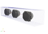
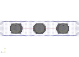
prospect view	$x_{1}x_{2}$ view
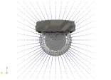
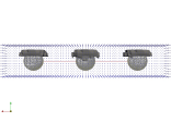
$x_{2}x_{3}$ view	$x_{3}x_{1}$ view

Figure 12: Test case iv). We present reconstruction of $\tilde{c}$ when $\max_{\Omega_{FEM}}c(x)=5.87$ for $\omega=40$ in (48) and noise level $\sigma=10\%$. The spherical wireframe of the isosurface with exact value of the function (54), corresponding to the value of the reconstructed $\tilde{c}$, is outlined by a thin line.

We use a post-processing procedure to get images of figures 4, 7, 10 - 12. This procedure is as follows: assume, that the functions $c^{m}(x)$ are our reconstructions obtained by the algorithm of section 5.3 where $m$ is the number of iterations in the conjugate gradient algorithm when we have stopped to compute $c(x)$. Then to get our final images, we set

$$\widetilde{c}^{m}(x)=\left\{\begin{array}[]{ll}c^{m}(x),&\text{ if }c^{m}(x)>P\max\limits_{\Omega_{FEM}}c^{m}(x),\\ 1,&\text{ otherwise. }\end{array}\right.$$ (51)

The values of the parameter $P\in(0,1)$ depends on the concrete reconstruction of the function $c(x)$ and plays the roll of a cut-off parameter for the function $c(x)$. If we choose $P\approx 1$ then we will cut almost all reconstruction of the function $c(x)$. Thus, values of $P$ should be chosen numerically. For tests i), ii) we have used $P=0.7$ and for case studies iii)-iv) we choose $P=0.5$.

Table 1. Computational results of the reconstructions in cases i)-iv) together with computational errors in achieved contrast in percents. Here, $\overline{N}$ is the final iteration number $m$ in the conjugate gradient method of section 5.3.

$\sigma=3\%$ $\sigma=10\%$ Case $\max_{\Omega_{FEM}}c_{\overline{N}}$ error, % $\overline{N}$ i) $2.21$ 44.75 $7$ ii) $2.07$ 48.25 $7$ iii) $5.91$ 1.5 $12$ iv) $5.09$ 15.2 $15$ Case $\max_{\Omega_{FEM}}c_{\overline{N}}$ error, % $\overline{N}$ i) $3.13$ 21.75 $9$ ii) $3.06$ 23.5 $9$ iii) $4.84$ 19.3 $16$ iv) $5.87$ 2.2 $18$

6.1 Test case i)

In this example we performed computations with two noise levels in data: $\sigma=3\%$ and $\sigma=10\%$. Figure 3 presents typical behavior of noisy backscattered data in this case. The results of reconstruction for both noise levels are presented in figure 4. We observe that the location of all inclusions in $x_{1}x_{2}$ direction is imaged very well. However, the location in the $x_{3}$ direction should still be improved.

It follows from figure 4 and table 1 that the imaged contrast in the function $c(x)$ is $2.21:1=\max_{\Omega_{FEM}}c_{7}:1$, where $n:=\overline{N}=7$ is our final iteration number in the conjugate gradient method. Similar observation is valid from figure 4 and table 1 for noise level 10 % where imaged contrast in the function $c(x)$ is $3.13:1=\max_{\Omega_{FEM}}c_{9}:1$, where $n:=\overline{N}=9$ is our final iteration number.

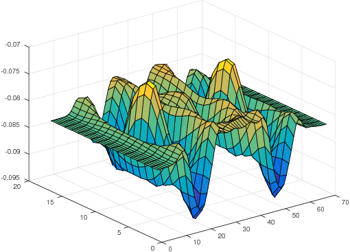
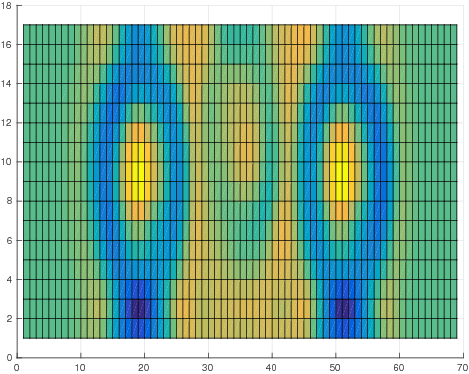
a) prospect view	b) $x_{1}x_{2}$ view

Figure 3: Test case i). Behavior of the noisy backscattered data at time $t=1.8$ with $\sigma=3\%$ in (50).

$\max\limits_{\Omega_{FEM}}c(x)=2.21,\sigma=3\%$	$\max\limits_{\Omega_{FEM}}c(x)=3.13,\sigma=10\%$
$x_{1}x_{3}$ view	$x_{1}x_{3}$ view

Figure 4: Test case i). Computed images of reconstructed $\tilde{c}$ for $\omega=40$ in (48) and for a different noise level $\sigma$ in (50). Bottom row present the respective $x_{1}x_{3}$ views.

6.2 Test case ii)

In this test, we have considered the same noise levels $\sigma$: $\sigma=3\%$ and $\sigma=10\%$, as in the test case i). The behavior of the noisy backscattered data in this case is presented in figure 5. Using figure 6 we observe that the difference in the amplitude of backscattered data between the cases i) and ii) is very small and, as expected, is located exactly at the place where the middle smallest inclusion of figure 2 is moved, This is because the difference in two geometries of figure 2 is only in the location of the small middle inclusion: in figure 2-b) this inclusion is moved more close to the backscattered boundary $\partial_{1}\Omega$ than in the figure 2-a).

The results of the reconstruction for both noise levels are presented in figure 7. It follows from figure 7 and table 1 that the imaged contrast in the function $c(x)$ is $2.07:1=\max_{\Omega_{FEM}}c_{7}:1$, where $n:=\overline{N}=7$ is our final iteration number in the conjugate gradient method when the noise level is 3 %. Similar observation is valid from figure 7 and table 1 for noise level 10 % where imaged contrast in the function $c(x)$ is $3.06:1=\max_{\Omega_{FEM}}c_{9}:1$, where $n:=\overline{N}=9$ is our final iteration number. Again, as in the case i) we observe that the location of all inclusions in $x_{1}x_{2}$ direction is imaged very well. However, location in $x_{3}$ direction should still be improved. We also observe that the smallest inclusion of figure 2-b) is reconstructed better than in the case i) since it is located closer to the observation boundary $\partial_{1}S$. Similar to [6, 7], in our future research, we plan to apply an adaptive finite element method which hopefully will improve the shapes and sizes of all inclusions considered in tests i) and ii).

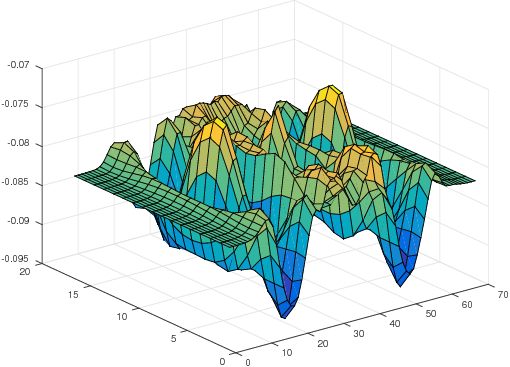
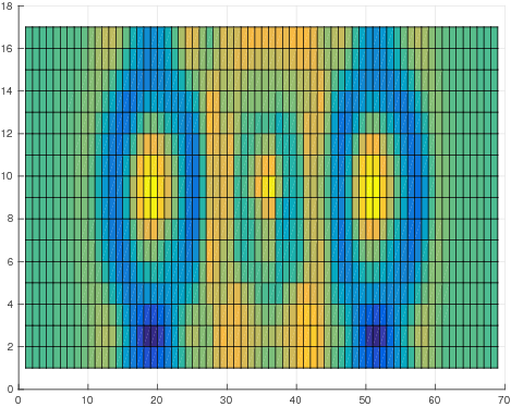
a) prospect view	b) $x_{1}x_{2}$ view

Figure 5: Test case ii). Behavior of the noisy backscattered data at time $t=1.8$ with $\sigma=3\%$ in (50).

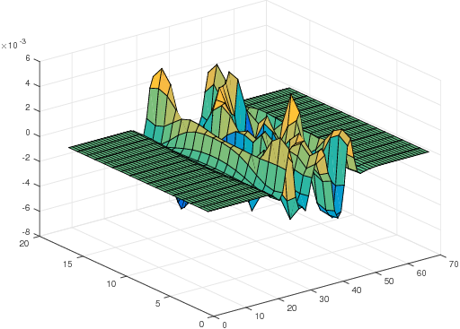
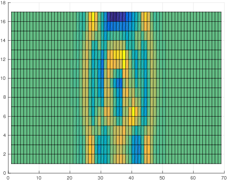
a) prospect view	b) $x_{1}x_{2}$ view

Figure 6: The difference of the noisy backscattered data at time $t=1.8$ in case studies i) and ii) when noise level is $\sigma=3\%$ in (50).

$\max\limits_{\Omega_{FEM}}c(x)=2.07,\sigma=3\%$	$\max\limits_{\Omega_{FEM}}c(x)=3.06,\sigma=10\%$
$x_{1}x_{3}$ view	$x_{1}x_{3}$ view

Figure 7: Test case ii). Computed images of reconstructed $\tilde{c}$ for $\omega=40$ in (48) and for different noise level $\sigma$ in (50). Bottom row present the $x_{1}x_{3}$ views.

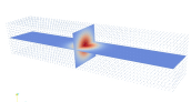
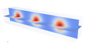
a) Test iii): horizontal and vertical slices	b) Test iv): horizontal and vertical slices
c) Test iii): horizontal and vertical slices	d) Test iv): horizontal and vertical slices
e) Test iii): threshold of the solution	f) Test iv): threshold of the solution

Figure 8: a), b). Slices of the exact Gaussian functions given by (52) and (54), respectively. c), d) Slices and e), f) thresholds of the reconstructions. Here, computations were done for the noise $\sigma=10\%$ and $\omega=40$.

6.3 Test case iii)

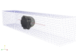
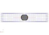
prospect view	$x_{1}x_{2}$ view
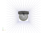
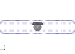
$x_{2}x_{3}$ view	$x_{3}x_{1}$ view

Figure 9: Test case iii). We present reconstruction of $\tilde{c}$ with $\max_{\Omega_{FEM}}c(x)=5.91$ for $\omega=40$ in (48) with noise level $\sigma=3\%$. The spherical wireframe of the isosurface with exact value of the function (52), which corresponds to the value of the reconstructed $\tilde{c}$, is outlined by a thin line.

prospect view	$x_{2}x_{3}$ view	$x_{1}x_{3}$ view

Figure 10: Test case iii). Computed images of reconstructed $\max_{\Omega_{FEM}}c(x)=4.84$ for $\omega=40$ in (48) and noise level $\sigma=10\%$. The spherical wireframe of the isosurface with exact value of the function (52), corresponding to the value of the reconstructed $\tilde{c}$, is outline by a thin line.

In this numerical test, we reconstruct the conductivity function $c(x)$ which is defined as follows

$$c(x)=1.0+5.0\cdot\exp^{-({x_{1}}^{2}/0.2+{x_{2}}^{2}/0.2+{x_{3}}^{2}/0.2)},$$ (52)

see Figure 8-a). In this test, we have used noisy boundary data $u_{\sigma}$ with $\sigma=3\%$ and $\sigma=10\%$ in (50). Note that a priori we have not assumed that we know the structure of this function, further we have assumed that we know the lower bound $c(x)\geq 1$ and that the reconstructed values of the conductivity belongs to the set of admissible parameters which is now defined as

$$\begin{split}M_{c}\in\{c\in C(\overline{\Omega})|1\leq c(x)\leq 10\}.\\ \end{split}$$ (53)

Figures 8-c), e) and 10 display results of the reconstruction of function given by (52) with $\sigma=10\%$ in (50). Quite similar results are obtained for $\sigma=3\%$ in (50), see figure 9. We observe that the location of the maximal value of the function (50) is imaged very well. It follows from figure 9 and table 1 that the imaged contrast in this function is $5.91:1=\max_{\Omega_{FEM}}c_{12}:1$, where $n:=\overline{N}=12$ is our final iteration number in the conjugate gradient method. Similar observation is valid from figure 10 and table 1 where the imaged contrast is $4.84:1=\max_{\Omega_{FEM}}c_{16}:1$, $n:=\overline{N}=16$. However, from these figures we also observe that because of the data post-processing procedure (51) the values of the background $1.0+5.0\cdot\exp^{-(x^{2}/0.2+y^{2}/0.2+z^{2}/0.2)}$ in (52) are not reconstructed but are smoothed out. Thus, we are able to reconstruct only maximal values of the function (52). Comparison of figures 8-c), e), 9, 10 with figure 8-a) reveals that it is desirable to improve shape of the function (52) in $x_{3}$ direction. Again, similar to [6, 7] we hope that an adaptive finite element method can refine the obtained images of figure 10 in order to get better shapes and sizes of the function (52) in all directions.

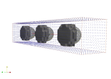
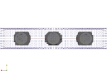
prospect view	$x_{1}x_{2}$ view
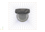
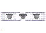
$x_{2}x_{3}$ view	$x_{3}x_{1}$ view

Figure 11: Test case iv). We present reconstruction of $\tilde{c}$ when $\max_{\Omega_{FEM}}c(x)=5.09$ for $\omega=40$ in (48) and noise level $\sigma=3\%$. The spherical wireframe of the isosurface with exact value of the function (54), which corresponds to the value of the reconstructed $\tilde{c}$, is outlined by a thin line.

6.4 Test case iv)

In our last numerical test we reconstruct the conductivity function $c(x)$ given by three sharp Gaussians such that

$$\begin{split}c(x)&=1.0+5.0\cdot\exp^{-((x_{1}+2)^{2}/0.2+{x_{2}}^{2}/0.2+{x_{3}}^{2}/0.2)}\\ &+5.0\cdot\exp^{-({x_{1}}^{2}/0.2+{x_{2}}^{2}/0.2+{x_{3}}^{2}/0.2)}+5.0\cdot\exp^{-(({x_{1}}-2)^{2}/0.2+{x_{2}}^{2}/0.2+{x_{3}}^{2}/0.2)},\end{split}$$ (54)

see Figure 8-b). In this test we again used the noisy boundary data $u_{\sigma}$ with $\sigma=3\%$ and $\sigma=10\%$ in (50). We assume that the reconstructed values of the conductivity belongs to the set of admissible parameters (53).

Figures 8-d),f), 11 and 12 show results of the reconstruction of function given by (54) for $\sigma=3\%$ and $\sigma=10\%$ in (50), respectively. We observe that the location of the maximal value of the function (54) is imaged very well. It follows from figure 11 and table 1 that when the noise level is $\sigma=3\%$ then the imaged contrast in this function is $5.09:1=\max_{\Omega_{FEM}}c_{15}:1$, where $n:=\overline{N}=15$ is our final iteration number in the conjugate gradient method. When the noise level is $\sigma=10\%$ then the imaged contrast is $5.87:1=\max_{\Omega_{FEM}}c_{18}:1,n:=\overline{N}=18$.

However, as in the case iii), the values of the background in (54) are not reconstructed but are smoothed out and we are able to reconstruct only maximal values of the three Gaussians in the function (54). Comparing figures 8-d),f), 11, 12 with figure 8-b) we see that it is desirable to improve shapes of the function (54) in $x_{3}$ direction.

7 Discussion and Conclusion

In this work, we have presented a computational study of the reconstruction of the conductivity function $c(x)$ in a hyperbolic problem (1) using Lagrangian approach and a hybrid finite element/difference method of [4]. As theoretical result, we have presented estimate of the norms between computed and regularized solutions of the Tikhonov functional via the $L_{2}$ norm of the Fréchet derivative of this functional or via the corresponding Lagrangian.

In our numerical tests, we have obtained stable reconstruction of the conductivity function $c(x)$ in $x_{1}x_{2}$-directions for frequency $\omega=40$ in the initialization of a plane wave (48) and for noise levels $\sigma=3\%,10\%$ in (50). However, size and shape on $x_{3}$ direction should still be improved in all test cases. Similar to [6, 7] we plan to apply an adaptive finite element method in order to get better shapes and sizes of the conductivity function $c(x)$ in $x_{3}$ direction.

Using results of table 1 we can conclude that the computational errors in the achieved maximal contrast are less in the case of reconstruction of smooth functions than in the reconstruction of small inclusions. This can be explained by involving of discontinuities in the reconstruction of small inclusions, as well as by having special geometry in these small inclusions: all of them have different sizes and locations inside $\Omega_{FEM}$, and thus, achieving the exact contrast becomes more difficult task in this case. The important observation is that when the scatters are of different size, especially when the smallest scatterer is located between larger ones, as in case studies i) and ii), we note that the smaller scatterer is better reconstructed when it is located near the observation boundary of the computational domain $\Omega_{FEM}$.

References

• [1] A. Bakushinsky, M. Y. Kokurin, A. Smirnova, Iterative Methods for Ill-posed Problems, Inverse and Ill-Posed Problems Series 54, De Gruyter, 2011.
• [2] A.B. Bakushinsky and M.Y. Kokurin, Iterative Methods for Approximate Solution of Inverse Problems, Springer, 2004.
• [3] L. Beilina, M. Cristofol and K. Niinimäki, Optimization approach for the simultaneous reconstruction of the dielectric permittivity and magnetic permeability functions from limited observations, Inverse Problems and Imaging, 9 (1) (2015), 1–25.
• [4] L. Beilina, Domain Decomposition finite element/finite difference method for the conductivity reconstruction in a hyperbolic equation, Communications in Nonlinear Science and Numerical Simulation, Elsevier, 2016, doi:10.1016/j.cnsns.2016.01.016
• [5] L. Beilina, K. Samuelsson, K. Åhlander, Efficiency of a hybrid method for the wave equation. Proceedings of the International Conference on Finite Element Methods: Three dimensional problems. GAKUTO international Series, Mathematical Sciences and Applications, 15 (2001).
• [6] L. Beilina and C. Johnson, A posteriori error estimation in computational inverse scattering, Mathematical Models in Applied Sciences, 1 (2005), 23-35.
• [7] L. Beilina, N. T. Thành, M. V. Klibanov, J. Bondestam-Malmberg, Reconstruction of shapes and refractive indices from blind backscattering experimental data using the adaptivity, Inverse Problems, 30 (2014), 105007.
• [8] L. Beilina, M.V. Klibanov, Approximate global convergence and adaptivity for coefficient inverse problems, Springer, New-York, 2012.
• [9] L. Beilina, M.V. Klibanov and M.Yu. Kokurin, Adaptivity with relaxation for ill-posed problems and global convergence for a coefficient inverse problem, Journal of Mathematical Sciences, 167 (2010), 279–325.
• [10] C. Bellis, M. Bonnet, and B. B. Guzina, Apposition of the topological sensitivity and linear sampling approaches to inverse scattering, Wave Motion, 50 (2013), 891–908.
• [11] S. C. Brenner and L. R. Scott, The Mathematical theory of finite element methods, Springer-Verlag, Berlin, 1994.
• [12] H. D. Bui, A. Constantinescu, and H. Maigre, An exact inversion formula for determining a planar fault from boundary measurements, Journal of Inverse and Ill-Posed Problems, 13 (2005), 553–565.
• [13] H. D. Bui, A. Constantinescu, and H. Maigre, Numerical identification of planar cracks in elastodynamics using the instantaneous reciprocity gap, Inverse Problems, 20, (2004), 993–1001.
• [14] Y. T. Chow and J. Zou A Numerical Method for Reconstructing the Coefficient in a Wave Equation Numerical Methods for Partial Differential Equations, 31, (2015), 289–307
• [15] M. Cristofol, S. Li, E. Soccorsi, Determining the waveguide conductivity in a hyperbolic equation from a single measurement on the lateral boundary, Mathematical control and related fields, 6, (3), 407-427, 2016.
• [16] G. C. Cohen, Higher order numerical methods for transient wave equations, Springer-Verlag, 2002.
• [17] Engquist B and Majda A, Absorbing boundary conditions for the numerical simulation of waves  Math. Comp. 31 (1977), 629–651.
• [18] H. W. Engl, M. Hanke and A. Neubauer, Regularization of Inverse Problems Boston: Kluwer Academic Publishers, 2000.
• [19] S. N. Fata and B. B. Guzina, A linear sampling method for near-field inverse problems in elastodynamics, Inverse Problems, 20, 2004), 713–736.
• [20] M. V. Klibanov, A. B. Bakushinsky, L. Beilina, Why a minimizer of the Tikhonov functional is closer to the exact solution than the first guess, Journal of Inverse and Ill - Posed Problems, 19 (1) (2011), 83–105.
• [21] O. A. Ladyzhenskaya, Boundary Value Problems of Mathematical Physics, Springer Verlag, Berlin, 1985.
• [22] O.Pironneau, Optimal shape design for elliptic systems, Springer-Verlag, Berlin, 1984.
• [23] PETSc, Portable, Extensible Toolkit for Scientific Computation, http://www.mcs.anl.gov/petsc/.
• [24] A. N. Tikhonov, A. V. Goncharsky, V. V. Stepanov and A. G. Yagola, Numerical Methods for the Solution of Ill-Posed Problems London: Kluwer, 1995.
• [25] WavES, the software package, http://www.waves24.com
• [26] R. Courant, K. Friedrichs and H. Lewy On the partial differential equations of mathematical physics, IBM Journal of Research and Development, 11(2) (1967), 215–234