DO–TH 15/13 QFET–2015–26

Rare Semileptonic Charm Decays

Stefan de Boer

Fakultät für Physik,
TU Dortmund, Otto-Hahn-Str.4, D-44221 Dortmund, Germany

An analysis of charm mesons decaying semileptonically via Flavor Changing Neutral Currents is presented. We calculate the Wilson coefficients within the Standard Model. A window in the decay distribution, where physics beyond the Standard Model could be measured is identified. Exemplary, we study effects of leptoquark models.

PRESENTED AT

The 7th International Workshop on Charm Physics (CHARM 2015)
Detroit, MI, 18-22 May, 2015

1 Introduction

Rare semileptonic charm decays, e.g. the decay $D\to P\ell\ell$, where $D=c\overline{q}$, $q\in\{u,d\}$, $P$ is a pseudoscalar meson and $\ell$ is a muon or an electron are induced by $c\to u\ell\ell$ transitions. Within the Standard Model (SM), the semileptonic decay of charm mesons via Flavor Changing Neutral Currents (FCNCs) is shown in Figure 1.

Figure 1: The $c\to u\ell\ell$ transition within the SM. The label $q_{d}$ denotes down-type quarks.

In the SM, FCNCs are loop and Glashow-–Iliopoulos-–Maiani (GIM) suppressed. The GIM suppression in $c\to u\ell\ell$ transitions is in particular effective due to the unitarity of the Cabibbo-–Kobayashi-–Maskawa (CKM) matrix $V$ and the small product $|V_{cb}^{*}V_{ub}|\approx 1.5\cdot 10^{-4}$. Thus, $c\to u\ell\ell$ induced decays are rare in the SM and sensitive to Beyond Standard Model (BSM) physics as BSM dynamics could induce larger effective couplings and additional structures compared to the SM. Rare semileptonic charm decays open windows to look for physics beyond the SM complementary to decays of $b$-quarks and $s$-quarks. Additionally, $c\to u\ell\ell$ transitions probe perturbative QCD as the mass of the charm quark is close to the scale $\Lambda_{\text{QCD}}$.

Experiments on rare charm decays were performed and are designed by several collaborations, e.g. LHCb, CMS, BaBar, Belle (II), CLEO-c and BESIII. The most stringent experimental limit to date is set on the mode $D^{+}\to\pi^{+}\mu^{+}\mu^{-}$ by the LHCb collaboration in 2013 reporting an upper limit on the fully integrated non-resonant branching fraction of [1]

$$\mathcal{B}^{\text{exp}}(D^{+}\to\pi^{+}\mu^{+}\mu^{-})<7.3\times 10^{-8}\quad(90\%\,\text{CL})\,.$$ (1)

Additionally, upper limits in the low $q^{2}$ bin ($0.250\,\text{GeV}\leq\sqrt{q^{2}}\leq 0.525\,\text{GeV}$) and in the high $q^{2}$ bin ($1.250\,\text{GeV}\leq\sqrt{q^{2}}$), where $q^{2}$ is the dilepton mass squared read [1]

$$\mathcal{B}^{\text{exp,low}}(D^{+}\to\pi^{+}\mu^{+}\mu^{-})<2.0\times 10^{-8}\quad(90\%\,\text{CL})\,,$$ (2)

$$\mathcal{B}^{\text{exp,high}}(D^{+}\to\pi^{+}\mu^{+}\mu^{-})<2.6\times 10^{-8}\quad(90\%\,\text{CL})\,.$$ (3)

Calculations of the $c\to u\ell\ell$ branching fractions were performed by several groups. Predictions for the fully integrated non-resonant SM branching fraction of $D^{+}\to\pi^{+}\mu^{+}\mu^{-}$ decays are given as

$$\mathcal{B}_{D^{+}\to\pi^{+}\mu^{+}\mu^{-}}^{\text{nr,SM}}=6\cdot 10^{-12}\quad\cite[cite]{[\@@bibref{}{Fajfer:2005ke}{}{}]}\,,$$ (4)

$$\mathcal{B}_{D^{+}\to\pi^{+}\mu^{+}\mu^{-}}^{\text{nr,SM}}=[4.59,8.04]\cdot 10^{-10}\quad\cite[cite]{[\@@bibref{}{Wang:2014uiz}{}{}]}\,.$$ (5)

Equations (4) and (5) differ by two orders of magnitude. This discrepancy persists in the predictions for the inclusive branching fractions

$$\mathcal{B}_{D^{+}\to X_{u}^{+}e^{+}e^{-}}^{\text{nr,SM}}=2\cdot 10^{-8}\quad\cite[cite]{[\@@bibref{}{Burdman:2001tf}{}{}]}\,,$$ (6)

$$\mathcal{B}_{D^{+}\to X_{u}^{+}e^{+}e^{-}}^{\text{nr,SM}}=6.0\cdot 10^{-10}\quad\cite[cite]{[\@@bibref{}{Fajfer:2005ke}{}{}]}\,,$$ (7)

whereas [5] gives a branching fraction consistent with equation (6).

Thus, we will do the following: We calculate the SM branching fractions within the framework of an effective theory and identify the differences in the calculations of [3], [4], [5] and [2]. Additionally, we look for measurable BSM effects in the decay distribution, e.g. due to leptoquark models.

2 SM Branching Fractions

In this section, we sketch the calculation of the SM branching fractions of the inclusive $c\to u\ell\ell$ decay and of the modes $D^{+}\to\pi^{+}\ell^{+}\ell^{-}$, where $\ell\in\{e,\mu\}$ [6], [7]. By means of an Operator Product Expansion (OPE) we write the leading order effective weak Lagrangian at the weak scale as [8]

$$\mathcal{L}_{\text{eff}}^{\text{weak}}|_{\mu\sim\mu_{W}}= {\frac{4G_{F}}{\sqrt{2}}\sum_{q\in\{d,s,b\}}V_{cq}^{*}V_{uq}}\left(C_{1}(\mu)Q_{1}^{(q)}(\mu)+C_{2}(\mu)Q_{2}^{(q)}(\mu)\right)\,,$$ (8)

where $G_{F}$ denotes the Fermi constant. The operators $Q_{i}^{(q)}$ read [9]

$$Q_{1}^{(q)}=(\overline{u}_{L}\gamma_{\mu_{1}}T^{a}q_{L})(\overline{q}_{L}\gamma^{\mu_{1}}T^{a}c_{L})\,,$$ (9)

$$Q_{2}^{(q)}=(\overline{u}_{L}\gamma_{\mu_{1}}q_{L})(\overline{q}_{L}\gamma^{\mu_{1}}c_{L})\,,$$ (10)

where $T^{a}$ denotes the $SU(3)$ generators. At the scale $\mu$, short-distance Wilson coefficients $C_{i}$ and the long-distance operators generated by light fields are factorized.

The Wilson coefficients are found by matching the SM Lagrangian onto the effective Lagrangian (8) at the weak scale. Thus, heavy fields are integrated out, e.g. in QCD at Next-to-Next-to-Leading Order [10]. The Wilson coefficients at lower scales are found via the solution of the Renormalization Group (RG) equation [11]. At the threshold of the mass of the bottom quark it is integrated out generating the additional operators $Q_{3-10}$ shown in Figure 2.

$Q_{3-6}\sim$   $Q_{7,8}\sim$   $Q_{9,10}\sim$

Figure 2: Pictorial representation of the additional operators due to the integration of the bottom quark. The label $q$ in the sum of $Q_{3-6}$ denotes light quark fields.

Thus, the Wilson coefficients $C_{1-10}(\mu_{c})$ at the charm scale are found by resumming logarithms to all orders in perturbation theory by means of the RG.

We calculate the matrix elements of the operators $\langle Q_{1-6,8}\rangle$ in terms of effective Wilson coefficients. The factorized hadronic matrix elements $\langle Q_{7,9,10}\rangle$ are parametrized via three form factors. The form factors are related within the Heavy Quark Effective Theory yielding one independent form factor $f_{+}$. We parametrize the form factor $f_{+}$ by means of the z-expansion, where the parameters are fitted to the experimentally measured $D\to\pi\ell\nu_{\ell}$ decay [12].

The calculation of the non-resonant SM branching fractions as sketched above yields [7]

$$\mathcal{B}_{D^{+}\to X_{u}^{+}e^{+}e^{-}}^{\text{nr,SM}}\approx 1\cdot 10^{-9}\,,$$ (11)

$$\mathcal{B}_{D^{+}\to X_{u}^{+}\mu^{+}\mu^{-}}^{\text{nr,SM}}\approx 2\cdot 10^{-10}\,,$$ (12)

$$\mathcal{B}_{D^{+}\to\pi^{+}\ell^{+}\ell^{-}}^{\text{nr,SM}}\approx 5\cdot 10^{-12}\quad(\ell\in\{e,\mu\})\,.$$ (13)

Our branching fractions (11)-(13) are consistent with equations (4) and (7) as calculated in [2]. Compared to the calculations in [4], [5] and [3] the primarily difference is due to the matching coefficients at the weak scale, e.g. [13]

$$C_{9}(\mu_{W})=\sum_{q\in\{d,s,b\}}V_{cq}^{*}V_{uq}C_{9,\text{IL}}^{(q)}\approx V_{cs}^{*}V_{us}\frac{-2}{9}\ln\frac{m_{s}^{2}}{m_{d}^{2}}\approx-0.29$$ (14)

which is vanishing in our matching. By means of equation (14) light quark fields are integrated out at the weak scale. This, is not consistent within the OPE factorization of scales. In particular, the logarithms as in $C_{9,\text{IL}}^{(q)}$ are resumed by means of the RG.

3 BSM Physics and Leptoquarks

We add the resonant modes in the decay distribution by parameterizing them in terms of a Breit-Wigner shape, where the $\omega$ and $\rho$ resonances are related as deduced in [2] and we take the experimental upper limit for the $\eta^{\prime}$ resonance. The $D^{+}\to\pi^{+}\mu^{+}\mu^{-}$ decay distribution is shown in Figure 3.

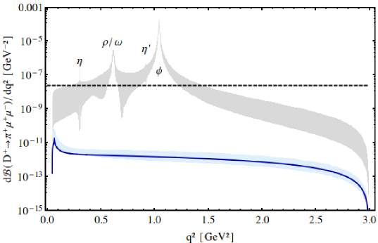
Figure 3: The $D^{+}\to\pi^{+}\mu^{+}\mu^{-}$ dilepton mass squared decay distribution. The solid blue curve is the non-resonant prediction at $\mu_{c}=\overline{m}_{c}$ and the light blue band its $\mu_{c}$-uncertainty. We find the gray resonant band by fitting the experimental branching fractions via a constant width Breit-Wigner shape and varying the relative strong resonant phases. The dashed black line is the binned non-resonant 90% CL experimental upper limit taken from [1]. Figure taken from [7].

In the SM, the branching fraction of the non-resonant mode is orders of magnitude smaller than the branching fraction of the resonant modes and likewise the current experimental upper limit. Yet, at high $q^{2}$ the difference between the SM prediction and the experimental limit opens a window to look for BSM physics. We predict the non-resonant SM branching fraction at high $q^{2}$ to be [7]

$$\mathcal{B}_{D^{+}\to\pi^{+}\mu^{+}\mu^{-}}^{\text{nr,SM}}\big{|}_{q^{2}\geq 1.525\,\text{GeV}^{2}}\approx 7.4\cdot 10^{-13}\;_{-14\%}{}^{+15\%}(\overline{m}_{s})\,_{-45\%}^{+136\%}(\mu_{c})\,_{-20\%}^{+27\%}(f_{+})\,,$$ (15)

where uncertainties ($\overline{m}_{c}/\sqrt{2}\leq\mu_{c}\leq\sqrt{2}\overline{m}_{c}$) larger than ten percent are given, but we neglect power corrections. The scale uncertainty is large due to a variation of $\mu_{c}$ close to $\Lambda_{\text{QCD}}$ and could be reduced via a calculation of the two-loop effective Wilson coefficient of $Q_{9}$ due to $\langle Q_{1,2}^{(d,s)}(\mu_{c})\rangle$.

Clearly, any experimental signal in the branching fraction at high $q^{2}$ would be due to physics beyond the SM, e.g. a leptoquark (LQ) model. Exemplary, we study effects of the low-energy scalar (3,3,-1/3) and vector (3,1,-5/3) LQ representations [14]

$$\lambda_{S_{3}}(\mathbf{Q}_{L}^{T}i\tau_{2}\vec{\tau}\mathbf{L}_{L})\cdot\vec{S_{3}}^{\dagger}\subset\mathcal{L}_{LQ}\,,$$ (16)

$$\lambda_{\tilde{V}_{1}}\overline{q}_{R}\gamma_{\mu}\ell_{R}(\tilde{V}_{1}^{\mu})^{\dagger}\subset\mathcal{L}_{LQ}\,,$$ (17)

where $\mathbf{Q}$ are SM quark doublets, $\mathbf{L}$ are SM lepton doublets and $\tau_{i}$ denote the Pauli matrices. Collider experiments constrain the LQ mass to be greater or similar than one TeV. The products of couplings $\lambda$ inducing $c\to u\mu\mu$ transitions are constrained by the experimental limits on the branching fractions of $D^{0}\to\mu^{+}\mu^{-}$ and $D^{+}\to\pi^{+}\mu^{+}\mu^{-}$ decays. As the scalar LQ model couples to quark doublets, its induced Wilson coefficients are additionally constrained by kaon decays. For that purpose, we take the hierarchical flavor pattern of [15] to link the recent data on lepton flavor non-universality in rare semileptonic bottom decays. The LQ induced decay distribution at high $q^{2}$ is shown in Figure 4.

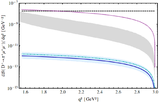
Figure 4: The $D^{+}\to\pi^{+}\mu^{+}\mu^{-}$ dilepton mass squared decay distribution at high $q^{2}$. The solid blue curve is the non-resonant SM prediction at $\mu_{c}=\overline{m}_{c}$ and the light blue band its $\mu_{c}$-uncertainty, the gray band shows the resonant modes and the dashed black line denotes the 90% CL experimental upper limit [1]. Additionally, the dotted purple curve represents the vector leptoquark model and the dot-dashed cyan curve is the scalar leptoquark model. Figure adopted from [7].

At high $q^{2}$, the vector LQ model could induce branching fractions close to the experimental upper limit and the scalar LQ model induced branching fractions would degenerate into the SM prediction.

4 Summary

We have presented a calculation of the $c\to u\ell\ell$ Wilson coefficients within the SM. The purpose of this calculation was to resolve discrepancies in the literature on the predictions for the non-resonant SM branching fractions. Our fully integrated prediction $\mathcal{B}_{D^{+}\to\pi^{+}\mu^{+}\mu^{-}}^{\text{nr,SM}}\sim 10^{-12}$ is orders of magnitude below the branching fraction of the resonant modes and likewise the current experimental upper limit $\mathcal{B}^{\text{nr,exp}}(D^{+}\to\pi^{+}\mu^{+}\mu^{-})\lesssim 10^{-8}$. Yet, at high $q^{2}$ a window is identified, where BSM physics could be measurable. Exemplary, we have studied effects of leptoquark models and found that a $SU(2)$-singlet vector leptoquark could induce branching fractions close to the current experimental limit.

ACKNOWLEDGEMENTS

I would like to thank the organizers for the wonderful conference. I am grateful to Gudrun Hiller, Bastian Müller and Dirk Seidel for a fruitful collaboration and Diganta Das for reading the manuscript. This project is supported by the DFG Research Unit FOR 1873 “Quark Flavour Physics and Effective Field Theories”.

References

- [1] R. Aaij et al. [LHCb Collaboration], Phys. Lett. B 724 (2013) 203 [arXiv:1304.6365 [hep-ex]].
- [2] S. Fajfer and S. Prelovsek, Phys. Rev. D 73 (2006) 054026 [hep-ph/0511048].
- [3] R. M. Wang, J. H. Sheng, J. Zhu, Y. Y. Fan and Y. G. Xu, Int. J. Mod. Phys. A 30 (2015) 12, 1550063 [arXiv:1409.0181 [hep-ph]].
- [4] G. Burdman, E. Golowich, J. L. Hewett and S. Pakvasa, Phys. Rev. D 66 (2002) 014009 [hep-ph/0112235].
- [5] A. Paul, I. I. Bigi and S. Recksiegel, Phys. Rev. D 83 (2011) 114006 [arXiv:1101.6053 [hep-ph]].
- [6] S. de Boer, B. Müller and D. Seidel, to appear, DO-TH 15/11, QFET-2015-27
- [7] S. de Boer and G. Hiller, arXiv:1510.00311 [hep-ph].
- [8] C. Greub, T. Hurth, M. Misiak and D. Wyler, Phys. Lett. B 382 (1996) 415 [hep-ph/9603417].
- [9] K. G. Chetyrkin, M. Misiak and M. Munz, Phys. Lett. B 400 (1997) 206 [Phys. Lett. B 425 (1998) 414] [hep-ph/9612313].
- [10] C. Bobeth, M. Misiak and J. Urban, Nucl. Phys. B 574 (2000) 291 [hep-ph/9910220].
- [11] M. Gorbahn and U. Haisch, Nucl. Phys. B 713 (2005) 291 [hep-ph/0411071].
- [12] Y. Amhis et al. [Heavy Flavor Averaging Group (HFAG) Collaboration], arXiv:1412.7515 [hep-ex].
- [13] T. Inami and C. S. Lim, Prog. Theor. Phys. 65 (1981) 297 [Prog. Theor. Phys. 65 (1981) 1772].
- [14] S. Davidson, D. C. Bailey and B. A. Campbell, Z. Phys. C 61 (1994) 613 [hep-ph/9309310].
- [15] I. de Medeiros Varzielas and G. Hiller, JHEP 1506 (2015) 072 [arXiv:1503.01084 [hep-ph]].