Towards an optimal flow: Density-of-states-informed replica-exchange simulations

Abstract

Replica exchange (RE) is one of the most popular enhanced-sampling simulations technique in use today. Despite widespread successes, RE simulations can sometimes fail to converge in practical amounts of time, e.g., when sampling around phase transitions, or when a few hard-to-find configurations dominate the statistical averages. We introduce a generalized RE scheme, density-of-states-informed RE (g-RE), that addresses some of these challenges. The key feature of our approach is to inform the simulation with readily available, but commonly unused, information on the the density of states of the system as the RE simulation proceeds. This enables two improvements, namely, the introduction of resampling moves that actively move the system towards equilibrium, and the continual adaptation of the optimal temperature set. As a consequence of these two innovations, we show that the configuration flow in temperature space is optimized and that the overall convergence of RE simulations can be dramatically accelerated.

Sampling the phase space of Hamiltonians to estimate thermodynamic properties is one of the fundamental problems in statistical physics. However, direct approaches often dramatically fail due to the presence of large free-energy barriers between different regions of phase space. While many methods have been proposed to address this challenge, few have had an impact as significant as the replica exchange (RE) method Geyer (1991); Lyubartsev et al. (1992); Hukushima and Nemoto (1996); Earl and Deem (2005). Indeed, since its introduction RE has established itself as a workhorse in atomistic and coarse-grained simulations and is currently used to investigate a large variety of systems in many areas ranging from statistical physics Hasenbusch et al. (2008); Yucesoy et al. (2012); Bittner and Janke (2006), over biology and chemistry Hansmann (1997); Gross et al. (2013); Tsai et al. (2005), to solid-state physics and materials science Falcioni and Deem (1999); Auer and Frenkel (2001); Chuang et al. (2005).

RE enhances the exploration of phase space by using a set of $N$ individual simulations (often called “walkers”) that evolve through Monte Carlo (MC) or molecular dynamics (MD) updates under different external parameters. For example, each walker might run at a different temperature $T_{i}$ ($1\leq i\leq N$), which is the situation we consider in the following (in this context, RE is often referred to as Parallel Tempering). After predefined time intervals $\tau_{\mathrm{RE}}$, the exchange of the current microstates between pairs of walkers is attempted and carried out with an appropriate probability; $W_{\mathrm{acc}}(U_{i},U_{j})=\min[1,\mathrm{e}^{\Delta\beta\,\Delta U}]$ in the case of canonical walkers, where $\beta_{i}=(k_{\mathrm{B}}T_{i})^{-1}$ are the inverse temperatures of the heat baths and $U_{i}$ the internal potential energies of the microstates. This exchange mechanism promotes configurational mixing by exposing replicas to external conditions (e.g., high temperatures) where free energy barriers can easily be overcome. It further provides a means for thermodynamic information to be transferred to conditions where the convergence of direct MC or MD simulations would require prohibitively long simulation times.

The exchange probabilities in RE strictly comply with detail balance, which ensures that the proper canonical distributions will be sampled at all temperatures. This property is extremely useful, because samples taken at each temperatures can be used without reweighting. It can however be restrictive, especially in the early stages of a simulation, when systems are far from equilibrium. This is related to the fact that conventional RE does not provide a natural mechanism to integrate and exploit information that becomes available during the simulation.

In this manuscript, we show how one such inexpensive and readily available source of information, namely, concurrent estimates of the density of states, $g(U)$, can significantly improve conventional RE. We leverage the (approximate) knowledge of $g(U)$ in two ways: first, we introduce a resampling operation akin to a Gibbs sampling move, which samples according to the $g(U)$-inferred canonical distribution over an ensemble of configurations previously visited by any replica; as we will show thereby explicitly steering the system toward equilibrium. Second, we use estimates of $g(U)$ to continuously improve the temperature set $\{T_{i}\}$. Because resampling breaks correlations along individual trajectories on each replica, the temperature set can be made optimal with respect to diffusion in temperature space Nadler and Hansmann (2007).

The enabling factor of our approach is the concurrent estimation of the density of states $g(U)$. While it can be obtained by a number of techniques Wang and Landau (2001); Laio and Parrinello (2002); Kim et al. (2006); Junghans et al. (2014), we here rely on ideas from the Adaptive Biasing Force (ABF) formalism Darve et al. (2008) for MD simulations. The key is to frame the problem as the estimation of the free energy $F_{\beta}(U)=-k_{\mathrm{B}}T\ln[g(U)\,\exp(-\beta U)]$ through its derivative $s$, which can be written in terms of microcanonical averages Darve et al. (2008) as:

$$s(U)=\frac{\mathrm{d}F}{\mathrm{d}U}=-\left\langle\frac{\mathrm{d}}{\mathrm{d}t}(w\cdot p)\right\rangle_{U}\,,$$ (1)

with $p$ being the vector of momenta and $w=\nabla U/(\nabla U\cdot\nabla U)$. Here, the derivative with respect to time is understood as a derivative along a micro-canonical trajectory. In practice, $\mathrm{d}(w\cdot p)/{\mathrm{d}t}$ is measured periodically (say every 100 timesteps) and stored with its corresponding value of $U$. We then use binned averages to reconstruct $s(U)$. By integration, we recover $F_{\beta}(U)$, and hence $g(U)$ . In an alternative representation, $s(U)$ can be used to define a microcanonical temperature observable: $T_{\mathrm{m}}(U)=T_{0}/(1-s(U))$, where $T_{0}$ is the heat-bath temperature. By integrating the thermodynamic relation $1/T_{\mathrm{m}}(U)=\mathrm{d}S(U)/\mathrm{d}U$, with $S(U)=k_{\mathrm{B}}\ln g(U)$, one reaches the same result. Note that if the momenta are unavailable, e.g., when using MC dynamics, a configurational temperature $T_{\mathrm{m}}(U)$ can be estimated based on structural data alone Rugh (1997); Butler et al. (1998); SM . The cost of estimating $s(U)$ is negligible in practice. An advantage of this approach is that the validity of Eq. (1) does not depend on the sampling being carried out in any particular ensemble: the only requirement is that the dynamics yield equal probabilities of observing different configurations with the same $U$. To minimize the impact of initial — potentially far-from-equilibrium — states on the estimator at later times, we introduce a memory time (much larger than all other time scales) after which measurements are discarded.

While in the ABF method Darve et al. (2008), $s(U)$ is used to create a multicanonical ensemble, we instead leverage it in g-RE in the following ways. While leaving the original RE mechanism untouched, we first introduce an additional, global resampling move (executed after time intervals $\tau_{\mathrm{resamp}}$) by which the microstate of a replica is resampled from the ensemble of configurations visited by any of its peers at any time in the past. In practice, this is enabled by a global configuration database populated by all walkers during the simulation. A configuration is selected from the database with a probability proportional to its estimated canonical weight $P_{\beta_{i}}(U)=g(U)\exp[-\beta_{i}U]$. This is akin to an approximate Gibbs sampling Liu (2002); Chodera and Shirts (2011). What is crucial here is that the $P_{\beta_{i}}(U)$ are inferred from global thermodynamic information, so that it can differ from the distribution locally sampled by the corresponding walker. In other words, this operation actively steers the distributions towards what is globally deemed equilibrium. It does so by allowing for the replication of thermodynamically relevant states, in contrast to conventional RE where configuration can only diffuse in configuration space. As will be shown below, resampling proves essential for convergence in the neighborhood of strong phase transitions and for the timely escape out of metastable states. One might, however, wonder whether g-RE produces correct statistics, as resampling does not a priori obey global balance when the configuration database is finite. In fact, the only requirement for correctness is that any two state with the same $U$ have the same probability of eventually being observed during an arbitrary long simulation.

As discussed in the Supplementary Materials below, this remains the case when resampling is introduced, as long as the samplers on each replicas (e.g., Langevin-MD or Metropolis MC) are ergodic and canonical in and of themselves. In that limit, $g(U)$, as obtained through Eq. 1 will converge to the correct value. From the knowledge of $g(U)$ and from a sample of observed configurations, any canonical quantity can then be obtained. It is however important to note that resampling introduces correlations between the configurations stored in the database at a specific point in time, and hence, potentially also between replicas. Our approach exploits these correlations to share information between replicas. However, resampling too frequently will lead to statistical ineficiencies. The optimal choice of $\tau_{\mathrm{resamp}}$ will be discussed in future works.

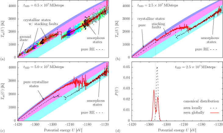
Figure 1: Convergence of $T_{\mathrm{m}}(U)$ at different simulation times: (a) shortly after the start of the run and after the first pure crystalline states have been discovered; (b) these states get replicated and move the spurious transition between pure and faulted states upwards in temperature; (c) after convergence of the g-RE scheme. The dots in (a) exemplarily show individual measurements, different colors correspond to different walkers (only a subset of data from every other walker is shown). The solid, red line shows $T_{\mathrm{m}}(U)$, the dashed black line the same obtained from an equivalent, conventional RE run for comparison. The shaded bands in panels (a) to (c) are guides to the eyes and denote the type of configurations predominantly found in each of these regions, as indicated by the different labels. Panel (d) shows the estimated canonical distribution $P_{\beta_{i}}(U)$, at the time corresponding to panel (b), as obtained from global data (solid, red line) compared to what would be inferred by an isolated walker trapped in faulted states (dotted, black line).

The availability of $g(U)$ also enables a second innovation: the continuous optimization of the temperature set $\{T_{i}\}$. The overall goal here is to minimize the round-trip time for replicas to wander between low and high temperatures. Much effort has been (and is still) dedicated to addressing this issue (see Refs. Rathore et al. (2005); Katzgraber et al. (2006); Trebst et al. (2006); Nadler and Hansmann (2007); Neuhaus et al. (2007); Patriksson and van der Spoel (2008); Bittner et al. (2008); Ballard and Wales (2014) for examples). From this body of work it emerges that performance is often characterized in terms of two key concepts: the average exchange acceptance probabilities $W_{\mathrm{acc}}(i,i+1)$ between pairs of neighboring temperatures, and the flow ratio $f(i)=n_{\mathrm{up}}(i)/[n_{\mathrm{up}}(i)+n_{\mathrm{down}}(i)]$, i.e., the fraction of replicas that diffuse up in temperature for a given walker $i$ (a replica is said to flow upwards if it visited the minimum temperature more recently than the maximum temperature, cf. Katzgraber et al. (2006); Trebst et al. (2006)). In the probability-centric view Nadler and Hansmann (2007); Neuhaus et al. (2007); Bittner et al. (2008), the objective is to find the $\{T_{i}\}$ such that $W_{\mathrm{acc}}(i,i+1)=\mathrm{const},\,\forall i$, the insight being that locally low acceptance probabilities would limit the free diffusion of replicas. In the flow-centric view Katzgraber et al. (2006); Trebst et al. (2006), the optimal set $\{T_{i}\}$ is such that $f(i)=1-[(i-1)/(N-1)]$ (for $T_{i}<T_{i+1},\,\forall i$), as this indicates an unimpeded flow of replicas. In contrast, the presence of a bottleneck would signal itself by comparatively flat regions separated by a sharp drop in $f(i)$. The two approaches have been contrasted by Nadler and Hansmann Nadler and Hansmann (2007) who showed that, in the special case where the dynamics on each replica become completely uncorrelated between exchange attempts, the optimal choice is to make the exchange probabilities constant, as this minimizes the round-trip time from the lowest to the highest temperatures. Furthermore, the flow ratio will also be linear in this case. In the current context, this limit can be approached by setting $\tau_{\mathrm{resamp}}=\tau_{\mathrm{RE}}$, as resampling decreases correlations (as long as $\tau_{RE}$ is not so short as to saturate the database with near-identical configurations). In g-RE, the optimal temperature set can easily be determined. Holding the minimal and the maximal temperatures fixed, we apply a bisection scheme until $\{T_{i}\}$ converges to a situation where

$$W^{\mathrm{m}}_{\mathrm{acc}}(P_{i+1},P_{i})=\int_{-\infty}^{\infty} P_{\beta_{i}}(U)\int_{-\infty}^{\infty}W_{\mathrm{acc}}(U,U^{\prime})$$

$$P_{\beta_{i+1}}(U^{\prime})\,\mathrm{d}U\mathrm{d}U^{\prime}=\mathrm{const},\;\forall i\,.$$ (2)

(see Supplemental Materials below for more details). Here also, the $P_{\beta_{i}}(U)$ are based on the current estimator of $g(U)$, and Eq. (2) can be evaluated numerically. This scheme is very fast in practice and does not require any preliminary calculation. We continuously readjust the temperatures at intervals $\tau_{\mathrm{adapt}}$, assisting convergence in situations where the walkers begin far from equilibrium. Note that adaption of the $\{T_{i}\}$ does not interfere with the averages necessary for the measurement of $s(U)$, as samples taken at different temperatures can be seamlessly integrated through Eq. (1).

We now demonstrate the performance of our method on a system of 500 silver atoms. The $N=71$ walkers are canonical molecular dynamics runs with a timestep of $\tau_{\mathrm{ts}}=2$ fs and the heat-bath temperatures are set by Langevin thermostats. Atoms interact via an embedded-atom potential Williams et al. (2006). The simulation cell is cubic and periodic boundary conditions are used in all directions. The minimum temperature is set to $T_{\mathrm{min}}=100$ K and the maximal to $T_{\mathrm{max}}=3500$ K. The particle density is fixed at $\rho=0.0585$ Å^-3, which corresponds to the density that minimizes the energy of the fcc crystal; the fcc configuration is therefore the putative global energy minimum for this system and should dominate up to the vicinity of the melting point, given that the thermal concentration of defects is expected to be vanishingly small. However, all walkers are initialized from a quenched liquid (amorphous) configuration. This choice makes the system a very good prototype of a case where the thermodynamically relevant configurations are unknown a priori and difficult to access. Indeed, from MD studies of metals (e.g., Ag Xiao and Hu (2006); Tian et al. (2008); Jian et al. (2010), Cu Liu et al. (2001), Ni Li et al. (2011), etc.) it is known that recovering the perfect crystalline state from the melt requires very slow cooling, otherwise the system remains trapped in amorphous states (at fast cooling) or in a mixture of fcc and hcp regions separated by stacking defects (at moderate cooling rates). In addition, the presence of a first-order transition (melting) within the range of temperatures makes this an extremely challenging system to study. Finally, since the thermal distributions of crystal defects is expected to be vanishingly small in a system of that size away from the immediate vicinity of the melting point, the validity of the results is easy to assess.

As illustrated in Fig. 1, the coupling of the different replicas through the estimator of $g(U)$ and the configurational database directs the evolution of the system towards thermal equilibrium by enabling the replication of thermodynamically relevant, crystalline states, in contrast to conventional RE where states are only exchanged. In that figure, we report the instantaneous estimators of the microcanonical temperature $T_{\mathrm{m}}(U)$ at different times in the simulation. In our example, the perfect crystalline states (upper, purple band) are essentially the only relevant ones below the melting point; they are, however, by construction not present in the early stages of the simulations. While, at lower temperatures, the system quickly leaves the amorphous region of phase space (lower, pale blue band) and crystallizes, most of these crystalline configurations initially contain stacking faults (middle, pink band) that take a very long time to anneal. Convergence of standard RE requires the perfect crystalline state to be independently found at least (and ideally much more than) $n_{<melt}$ times (the number of walkers for which $T_{i}<T_{\mathrm{melt}}$). The rate at which this occurs hence controls the convergence speed; from standard RE we infer this rate to be of the order $10^{8}\,\mathrm{s}^{-1}$ and the convergence would require approximately $2.5\times 10^{8}$ MD steps. In contrast, resampling enables the replication of the pure crystalline state as soon at it is found once by any replica. As illustrated in Fig. 1d, this occurs because the global estimate of $g(U)$ eventually contains contributions from the crystalline region that are locally invisible to a walker trapped in faulted states. Computational gains follow because the probability of resampling a crystalline state significantly exceeds that of a replica independently finding it.

The same is true around the melting transition, which is initially biased to lower temperatures due to the initialization from a quenched liquid (note that the melting point at constant volume is much higher than the triple point). Before equilibration, a spurious transition between perfect crystals and faulted states (the sudden drop in $T_{\mathrm{m}}(U)$ at low energies) is observed and the melting temperature is underestimated. This is illustrated in Fig. 1 a–b (red, solid lines). A particular advantage of continuous temperature adaptation is that the temperature set remains nearly optimal at all times, even as the position of the (spurious or real) phase transitions evolve during convergence. With g-RE we observe convergence at $t_{\mathrm{MD}}\approx 4\times 10^{7}$ MD steps, while conventional RE, even with temperature adaptation (black, dashed lines), still mainly samples faulted states. The temperature adaptation scheme is very robust and converges quickly, even for a poor choice of the initial set $\{T_{i}\}$ (see below).

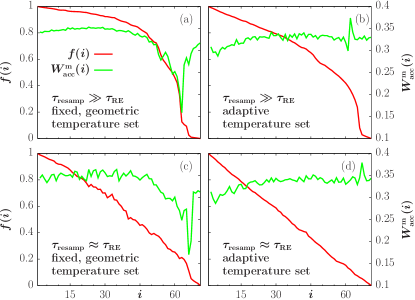
Figure 2: Measured RE acceptance rates ($W_{\mathrm{acc}}^{\mathrm{m}}(i,i+1)$; green curves) and fraction of replicas diffusing from the lowest to the highest temperature ($f(i)$; red curves) for the 500 Ag atoms system. (a,c) fixed, geometric temperature set (b,d) adaptive temperature set; (a,b) non-ergodic sampler: $\tau_{\mathrm{resamp}}\gg\tau_{\mathrm{RE}}$, (c,d) ergodic sampler: $\tau_{\mathrm{resamp}}\approx\tau_{\mathrm{RE}}$.

Finally, Fig. 2 shows how the introduction of global resampling at time scales comparable to the RE exchange time ($\tau_{\mathrm{resamp}}\approx\tau_{\mathrm{RE}}\sim 10^{2}\tau_{\mathrm{ts}}$) and an adaptive temperature set results in an optimal flow of the replica through temperature space, i.e., both constant $W_{\mathrm{acc}}^{\mathrm{m}}(i,i+1)$ and linear $f(i)$ are observed (Fig. 2 d). The measured round-trip times ($\tau_{\mathrm{rt}}^{\mathrm{m}}\approx 14000\,\tau_{\mathrm{RE}}$) are in perfect agreement with measured round-trip times for a purely random exchange process with corresponding exchange probabilities, which here correspond to the optimal limit Nadler and Hansmann (2007). As show in Fig. 2 a-c, these two conditions can only be obeyed when using both temperature adaptation and resampling. In this sense, our work integrates earlier efforts  Bittner et al. (2008); Trebst et al. (2006); Katzgraber et al. (2006), where either constant exchange times, exchange rates, or the optimal flow had to be sacrificed.

In conclusion, we introduce a general scheme, g-RE, that can dramatically improve the efficiency of RE simulations. The method is based on the idea of informing RE simulations with estimators of the density of states $g(U)$ gathered on the fly. This allows for two key improvements: the introduction of a global resampling move that guides the system towards equilibrium and causes a dramatic reductions of correlation times of the sampling, and the on-the-fly determination of an optimal temperature set that simultaneously achieves constant exchange probabilities and linear flow ratio. We expect our method to be particularly useful for any system with dominant but hard to access states or around strong first-order transitions. So far, there have been two approaches to such problems: either to change the ensemble (see Neuhaus et al. (2007); Kim et al. (2010) for examples) or to introduce global MC trial moves. In the former case, one often chooses to work in the multicanonical ensemble where $P(U)=\mathrm{const}$; creating such an ensemble is in fact a common way to leverage the knowledge of $g(U)$. This approach, however, is not optimal for the system reported here, because even though that ensemble is free from gradients of $F(U)$, the energy landscape locally remains extremely rough, thereby severely limiting the diffusivity in $U$. Using diffusion in $T$-space to promote mixing proved a more efficient alternative. Nonetheless, it still required the introduction of a global move to insure convergence. We here proposed a generic solution for constructing such a global move that does not require any a priori information about the system. We hence expect this approach to be useful for a wide range of systems and to also be applicable to RE schemes using other ensembles Gross et al. (2013); Sugita and Okamoto (2000); Kim et al. (2012); Vogel et al. (2013, 2014); Auer and Frenkel (2001).

Supplemental Material

Microcanonical temperature measurements

In this work we rely on methods that use measurements of temperature-like observables in order to estimate the derivative of the entropy (or, equivalently, of the density of states) with respect to energy. For example, the microcanonical temperature can be written in terms of configurational properties as

$$\frac{1}{k_{B}T_{\mathrm{conf}}(U)}=\left\langle\nabla\cdot\left(\frac{\nabla U}{\nabla U\cdot\nabla U}\right)\right\rangle_{U}\,$$ (3)

where $\langle\ldots\rangle_{U}$ is the average over states with a given potential energy $U$ Rugh (1997); Butler et al. (1998). For canonical averages or for very large system sizes, $T_{\mathrm{conf}}(U)$, measured from configurations in a heat-bath at constant temperature, is equal to just that canonical temperature Butler et al. (1998); Allen and Quigley (2013). Another way of estimating $\partial S/\partial U$ is based on thermodynamic integration using time derivatives, as derived in the context of the adaptive biasing force (ABF) method Darve et al. (2008). By using the potential energy as the ’order parameter’, $T_{\mathrm{m}}(U)=(\partial S(U)/\partial U)^{-1}$ can be estimated via

$$T_{\mathrm{ABF}}(U)=T_{0}/(1-s(U))\,,$$ (4)

where $T_{0}$ is the heat-bath temperature of the particular canonical-ensemble MD walker and with

$$s(U)=-\left\langle\frac{\mathrm{d}}{\mathrm{d}t}\left(\frac{\nabla U}{\nabla U\cdot\nabla U}\right)\cdot p\right\rangle_{U}\,,$$ (5)

where $p$ are the particle momenta. In contrast to Eq. (3), we do not need to calculate second derivatives of the potential energy, but only a time-derivative obtained in finite-difference form using a constant-energy MD timestep. This can be much less costly, especially for a complex many-body potentials, such as the one used in our work. However, if $p$ are not available, in a MC simulation, for example, one can instead use $T_{\mathrm{conf}}(U)$. In Fig. 3 we show raw measurements $T^{\prime}$ that contribute to the averages in Eqs. (3) and (4). Every data point corresponds to measurements of $T^{\prime}_{\mathrm{ABF}}$ and $T^{\prime}_{\mathrm{conf}}$ for one particular microstate sampled during the run. An extremely good agreement can be seen for both observables, not only with respect to each other but also with respect to the canonical reference temperatures indicated by the dotted lines. After carrying out the averages, we do not see any difference in the results of our simulations when using either of the observables and make our choice solely based on the computational performance.

As a valuable side-product, note that since $T_{\mathrm{m}}(U)$ is measured, the results are readily available for a microcanonical analysis of finite-size phase transitions Junghans et al. (2006); Schnabel et al. (2011).

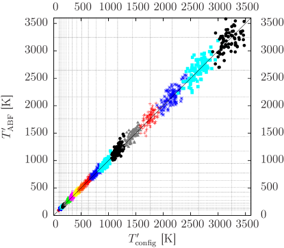
Figure 3: $T_{\mathrm{config}}$ vs. $T_{\mathrm{ABF}}$ for one example g-RE run with a fixed temperature set for the $N=500$ Ag system. Black, diagonal line: $T_{\mathrm{config}}=T_{\mathrm{ABF}}$ to guide the eye; Dotted lines: individual reference temperatures $T_{i}$. See text for details.

Determination of temperature sets

The transition (exchange) probability between two energy distributions $P_{i+1}$ and $P_{i}$ corresponding to different temperatures $\beta_{i}$ and $\beta_{i+1}$ takes the form

$$W^{\mathrm{tot}}_{\mathrm{acc}}(P_{i+1},P_{i})=\!\!\iint_{-\infty}^{\infty}\!\!P_{i}(U)W_{\mathrm{acc}}(U,U^{\prime})P_{{i+1}}(U^{\prime})\,\mathrm{d}U\mathrm{d}U^{\prime}.$$ (6)

$W_{\mathrm{acc}}(U,U^{\prime})$ is the usual acceptance probability for a replica exchange in canonical parallel tempering simulations: $W_{\mathrm{acc}}(U,U^{\prime})=\min[1,\mathrm{e}^{\Delta\beta\Delta U]}$, with $\Delta\beta$ being the difference in inverse temperature and $\Delta U$ the energy difference of the corresponding replicas. The integral in Eq. (6) is evaluated numerically as a sum over histogram bins. Recalling that $g(U)$ is used to calculate the energy distributions $P_{i}(U)=g(U)\exp[-\beta_{i}U]$, it is clear that the integrand takes non-negligible values only in a limited energy range, and hence that the bounds of the integrals can be restricted in practice. For example, the estimator of $g(U)$ is zero (by construction) at energies lower than the lowest energy observed by any replica, hence so is $P_{i}(U)=g(U)\exp[-\beta_{i}U]$. Similarly, at high energies, the Boltzmann factor leads to a rapid decay of $P_{i}(U)$, so that the integral can be truncated when $P_{i}(U)$ becomes negligible.

To find the optimal temperature set, we first (arbitrarily) select a target exchange probability $c_{t}$ and set $\beta_{1}=1/k_{B}T_{\mathrm{min}}$. We then successively apply a binary search (also known as interval halving method or bisection method; a standard method in numerical analysis Burden and Faires (1985)) to neighboring pairs of walkers to find $\beta_{i+1}$ such that $W^{\mathrm{tot}}_{\mathrm{acc}}(P_{i+1},P_{i})=c_{t}$. In practice, we first bracket the interval of $\beta_{i+1}$ that contains the solution to $W^{\mathrm{tot}}_{\mathrm{acc}}(P_{i+1},P_{i})=c_{t}$, and then apply a conventional binary search to identify the precise value. Given that the number $N$ of replicas is constant, a given value of $c_{t}$ implies a given value of $T_{N}$. To ensure that we always cover the same temperature range, we then apply an additional bisection scheme where we determine $c_{t}$ such that $T_{N}$ falls within a small range around the targeted maximal temperature $T_{\mathrm{max}}$. That is, whenever $T_{N}$ turns out to be too small we decrease $c_{t}$ (and vice versa), in ever smaller amounts Burden and Faires (1985) and repeat the procedure described above. Of course, if the converged $c_{t}$ is too small, one should increase the number of replicas $N$. Note that Eq. (2) (in the main article) only needs to be satisfied to some moderate precision to reap most of the performance benefits. Therefore, the tolerance in the bisection scheme, i.e., the range around the target value which is acceptable, can be adjusted. In all our simulations we observed that the determination of the optimal temperature set required only a negligible amount of computing time compared to the cost of actual MD, even though one evaluates a double-integral within a double-bisection scheme.

To emphasize the robustness of our scheme, we choose a far-from-optimal initial set $\{T_{i}\}$ for the run shown in Fig. 1 in the main article. About half of the walkers start at $T_{\mathrm{min}}$, the other half at $T_{\mathrm{max}}$; where there is, for all practical purposes, no overlap at all between the corresponding canonical distributions. Furthermore, recall that all walkers start with the same initial configuration. Still, the temperature set spreads out rapidly (see Fig. 4, in analogy to corresponding figures in Refs. Trebst et al. (2006); Katzgraber et al. (2006)) so that the walkers cover the whole range of temperatures and energies after a few adaptation steps. This illustrates that the method does not depend on the availability of any prior information on the system – in particular, no assumption or pre-estimation of the temperature set is necessary – and that it is very robust against even extreme choices of initial conditions.

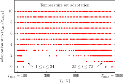
Figure 4: Convergence of the temperature set $\{T_{i}\}$ after an initialization where every walker starts either at the lower or the upper end of the total temperature range. The plot shows the evolution of $\{T_{i}\}$ during the first ten adaptation steps; after very few steps, the simulation optimally covers the whole temperature range. Data measured during the same simulation run shown in Fig. 1 in the main article.

Convergence to the canonical distribution

Despite of the fact that the g-RE procedure is history-dependent, i.e., that the result of the resampling depends on the previous history of the simulation through the content of the database, the method nonetheless converges to the canonical distribution. This can be seen by first considering a simpler situation: a single walker evolving through a canonical sampler and a database resampler. In this case, our database resampling procedure becomes:

• Sample a new configuration from the database

• Propagate for some time $\Delta t$ with a canonical sampler

• Insert the current configuration back into the database

• If the number of configuration in the database exceeds $M$, remove an element at random. Equivalently, old configurations could be purged from the database after a set time (as done in the manuscript).

• Repeat

Following this prescription, after $N$ cycles of the algorithm, every member of the database is the product of a proper time evolution. Indeed, from the perspective of individual configurations, they are randomly sampled, propagated for some time t with a canonical sampler, and then replaced in the database, i.e., they are the product of an unbiased sequence of propagation with the correct dynamics. However, because the configurations in the database are correlated, resampling from the same database does not produce independent canonical samples. For example, consider the case $M=2$: both configurations are now likely to be extremely similar if the propagation time $\Delta t$ is short. As we do not require independence, this is not an issue for g-RE in practice.

The second crucial point is that the “age” of the configurations in the database, i.e., the total (aggregate) amount of time they were propagated for, scales with the total simulation time. Therefore, in spite of correlations between individual entries, the sampling from the database over long times will be correct. Introducing a memory time after which configurations are dropped, as we did in the manuscript, directly imposes such a condition: “young” configurations cannot persist in the database by construction. Numerical simulations of the random deletion procedure demonstrate that this is also true there, to a remarkable extend. In fact, the mean age of a configuration is $\sim N\Delta t/M$, as can be intuitively expected. What is perhaps surprising is that the standard deviation of the age is a time ($N$)-independent constant that scales as $M^{1/2}$, i.e., the relative fluctuation (standard deviation of the age over the average age) vanishes at large $N$. Results for a memory size of 100 are shown in Fig. 5.

Figure 5: Statistics of the age of configurations in the database vs. $N$ for $M=100$.

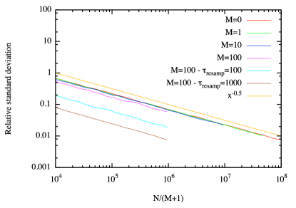
Figure 6: Relative standard deviation (w.r.t. the average) of the position $x$ of a walker for various memory size and resampling times. Unless otherwise specified, the resampling time is 1.

This shows that, while the average age of each configuration in the database is smaller than $N$, it scales with simulation time, and it is exceedingly unlikely that a very “young” configuration will be sampled. Taken together with the fact that each one of them is the product of a proper time evolution, this shows the above procedure yield a canonical sampler over long enough times. In the worst case (when $\Delta t$ is small) the configurations in the database will form a tight bundle in phase space. However, the bundle itself will evolve according to proper dynamics. Therefore, sampling from the database will yield unbiased canonical results over long times, so that we have an equal probability of sampling from the set of states with the same potential energy. As discussed in the manuscript, this is the only requirement for g-RE to be a valid sampler. However one should not expect multiple samples obtained from the database at the same time to be independent. Note that the same argument translates directly to the RE case, i.e., each configuration in the database taken alone, is a the product of proper dynamics whose age scales with the simulation time. We note that the situation appears problematic in the infinite $M$ limit or in the infinite memory time limit. As this is not a situation we have to confront in practice (because of finite computer memory), we do not explore that limit further.

The above discussion has been demonstrated using direct numerical simulations. We now consider a two-replica case. For simplicity, the system is a 1D square well in $0<x<1$. Given the flat energy landscape, the temperature is irrelevant, so doing RE would yield acceptance with unit probability and thus would yield identical results. The dynamics are carried out with Metropolis MC with a Gaussian proposal distribution of standard deviation 0.01. Unless otherwise noted, we carry out only one MC step between database resampling ($\tau_{\mathrm{resamp}}=1$). In Fig. 6, we report the relative standard deviation (the standard deviation over the average) of an histogram of the visited positions of one of the walkers as a function of $N/(M+1)$ for $M=0$ (standard MC), $1$, $10,$ and $100$. Note that each walker populates its own database but can only sample from the database of the other walker (which is equivalent to the setup used in the manuscript). Since the canonical distribution is uniform, convergence is indicated by a vanishing relative deviation at long times. As shown in the figure, all cases converge at roughly the same rate once the average age in the database is accounted for. Note that, because of decreased correlations due to the larger database, the $M=100$ case is converging even faster than expected from simple scaling arguments. Indeed, running the same case but resampling only every 100 or 1000 MC steps, thereby further limiting the correlation between entries in the database, yields an even faster convergence. Eventually, in the limit where the resampling time exceeds the ergodic relaxation time of the dynamics, the standard MC results (vs. $N$, not $N/M$ as plotted) are recovered, which is the expected behavior.