Molecular machines operating on nanoscale: from classical to quantum

Abstract

The main physical features and operating principles of isothermal nanomachines in microworld are reviewed, which are common for both classical and quantum machines. Especial attention is paid to the dual and constructive role of dissipation and thermal fluctuations, fluctuation-dissipation theorem, heat losses and free energy transduction, thermodynamic efficiency, and thermodynamic efficiency at maximum power. Several basic models are considered and discussed to highlight generic physical features. Our exposition allows to spot some common fallacies which continue to plague the literature, in particular, erroneous beliefs that one should minimize friction and lower the temperature to arrive at a high performance of Brownian machines, and that thermodynamic efficiency at maximum power cannot exceed one-half. The emerging topic of anomalous molecular motors operating sub-diffusively but highly efficiently in viscoelastic environment of living cells is also discussed.

I Introduction

Myriad of miniscule unseen in standard classical optical microscopes molecular nanomotors operate in living cells doing various tasks while utilizing metabolic energy, stored e.g. in ATP molecules maintained at out-of-equilibrium concentrations, or in nonequilibrium ion concentrations across biological membranes. And also vice versa they replenish the reserves of metabolic energy using other sources of energy, e.g. light by plants, or energy of covalent bonds of various food molecules by animals Pollard et al. (2008). The main physical principles of their operation are more or less understood by now Hill (1989); Nelson (2003), even if hardly one can state at present that the work of a single particular molecular motor, e.g. a representative of a large family of kinesin motors is understood and described in all finest statistico-mechanical detail. The advances and perspectives of nanotechnology compel us humans to devise our own nanomotors Kay et al. (2007); Erbas-Cakmak et al. (2015); Cheng et al. (2015). We do believe that learning from nature can help to make the artificial nanomotors highly efficient, and maybe even better than natural. On this way, to understand the main physical operating principles within the simplest minimalist physical models can help a lot indeed.

First of all, any periodically operating motor or engine requires a working body undergoing cyclic changes and a source of energy to drive such cyclic changes. Furthermore, it should be capable to do a useful work on external bodies. In case of thermal heat engines, the source of energy is provided by a heat exchange with two heat reservoirs or bathes at different temperatures $T_{1}$, and $T_{2}>T_{1}$ with the maximally possible Carnot efficiency $\eta_{C}=1-T_{1}/T_{2}$ Callen (1985). This very famous textbook result of classical thermodynamics or, better, thermostatics is to be modified, when the heat flows are considered in time. Then, for infinitesimally slow heat flows occurring yet in finite time, one obtains the Curzon and Ahlborn result $\eta_{CA}=1-\sqrt{T_{1}/T_{2}}\leq\eta_{C}$ Callen (1985); Curzon and Ahlborn (1975). The analogy with heat engines is, however, rather misleading for isothermal engines operating at the same temperature, $T_{1}=T_{2}$. Here, the analogy with electrical motors is much better. It becomes almost literal in the case of rotary ATP-synthase Yoshida et al. (2001) or flagellar bacterial motors – the electrical nanomotors of living cells, – where the energy of proton electrochemical gradient (an electrochemical rechargeable battery) is used to synthesize ATP molecules out of ADP and the orthophosphate $\rm P_{i}$ (the useful work done), in the case of ATP-synthase, or to produce mechanical motion by flagellar motors Pollard et al. (2008); Nelson (2003). Such a nanomotor as ATP-synthase can operate also in reverse Yoshida et al. (2001), and the energy of ATP hydrolysis can be used to pump protons against their electrochemical gradient to recharge “the battery”. Such and similar nanomotors can operate with isothermal thermodynamic efficiency, defined as the ratio of useful work done to the input energy spent, close to one, at ambient temperatures in a highly dissipative environment. This is a first counter-intuitive remarkable feature, which needs to be explained. It is easy to derive this result within a simplest model (see below) for an infinitesimally slow operating motor, at zero power. At the maximum power, at a finite speed, the maximal thermodynamic efficiency within such a model is one-half. This is still believed by many to be the maximally possible thermodynamic efficiency of isothermal motors at maximum power, in principle, as a theoretical bound. However, this belief born in underestimating the role played by thermal fluctuations in nonlinear stochastic dynamics and the role of fluctuation-dissipation theorem or FDT on nano- and microscale, is generally wrong. It is valid only for some particular dynamics, as we shall clarify below giving three counter-examples to it. The presence of strong thermal fluctuations at ambient temperatures, playing a constructive and useful role, is a profound physical feature of nanomotors, as compare with macroscopic motors of our everyday experience. One requires to understand and to develop intuition for this fundamental feature. Nanomotors are necessarily Brownian engines, very differently from macroscopic ones.

II Fluctuation-dissipation theorem, the role of thermal fluctuations

Motion in any dissipative environment is necessarily related to dissipation of energy. Particles experience a frictional force, which in a simplest case of Stokes friction is linearly proportional to the particle velocity with a viscous friction coefficient which will be denoted as $\eta$. If the corresponding frictional energy losses would not be compensated by an energy supply, the motion would eventually stop. However, this never happens in microworld for micro- or nanosized particles. Their stochastic Brownian motion can persist forever even at thermal equilibrium. The energy necessary for this is supplied by thermal fluctuations. Therefore, friction and thermal noise are intimately related which is a physical context of fluctuation-dissipation theorem Kubo (1966). Statistical mechanics allows to develop a coherent picture to rationalize this fundamental feature of Brownian motion. We start with some generalities which can be easily understood within a by now standard dynamical approach to Brownian motion that can be traced back to pioneering contributions by Bogolyubov Bogolyubov (1945), Ford, Kac, Mazur Ford et al. (1965, 1988), and others. Consider a Brownian particle with mass $M$, coordinate $x$, and momentum $p$. It is subjected to a regular dynamical force $f(x,t)$, as well as frictional and stochastically fluctuating forces of the environment. These later ones are modeled by an elastic coupling of this particle to a set of $N$ harmonic oscillators with masses $m_{i}$, coordinates $q_{i}$, and momenta $p_{i}$. We take this coupling in the form $V_{\rm int}=\sum_{i=1}^{N}\kappa_{i}(x-q_{i})^{2}/2$, with spring constants $\kappa_{i}$. This is a standard mechanistic model of nonlinear classical Brownian motion known within quantum dynamics also as Caldeira-Leggett model Caldeira and Leggett (1983) upon a modification of the coupling term, or making a canonical transformation Ford et al. (1988). Both classically and quantum-mechanically Ford et al. (1988) (in Heisenberg picture) the equations of motion read

$$\dot{x} = p/M,$$

$$\dot{p} = f(x,t)-\sum_{i=1}^{N}\kappa_{i}(x-q_{i}),$$ (1)

$$\dot{q}_{i} = p_{i}/m_{i},$$

$$\dot{p}_{i} = \kappa_{i}(x-q_{i})\;.$$ (2)

In quantum case, $x$, $q_{i}$, $p$, $p_{i}$ are operators obeying commutation relations $[x,p]=i\hbar$, $[q_{k},p_{j}]=i\delta_{kj}\hbar$, $[x,q_{i}]=0$, $[p,p_{i}]=0$. Force $f(x,t)$ is also operator. Using Green function of harmonic oscillators the dynamics of bath oscillators can be excluded (projection of hyper-dimensional dynamics on (x,p) plane) and presented further merely by the initial values $q_{i}(0)$ and $p_{i}(0)$. This results in a Generalized Langevin Equation (GLE) for the motor variables

$$M\ddot{x}+\int_{0}^{t}\eta(t-t^{\prime})\dot{x}(t^{\prime})dt^{\prime}=f(x,t)+\xi(t),$$ (3)

where

$$\eta(t)=\sum_{i}\kappa_{i}\cos(\omega_{i}t),$$ (4)

is a memory kernel and

$$\xi(t)=\sum_{i}\kappa_{i}\left([q_{i}(0)-x(0)]\cos(\omega_{i}t)+\frac{p_{i}(0)}{m_{i}\omega_{i}}\sin(\omega_{i}t)\right)\;$$ (5)

is a bath force, where $\omega_{i}=\sqrt{\kappa_{i}/m_{i}}$ are the frequencies of bath oscillators. Eq. (3) is still a purely dynamical equation of motion which is exact. The dynamics of $[x(t),p(t)]$ is completely time-reversible for any given $q_{i}(0)$ and $p_{i}(0)$ by derivation, unless the time-reversibility is dynamically broken by $f(x,t)$, or by boundary conditions. Hence, time-irreversibility within a dissipative Langevin dynamics is in the first line a statistical effect due to averaging over many trajectories. Such an averaging cannot be undone, i.e. there is no way to restore a single trajectory from their ensemble average. Consider further first a classical dynamics. Let us choose initial $q_{i}(0)$ and $p_{i}(0)$ from a canonical hyper-dimensional Gaussian distribution $\rho(q_{i}(0),p_{i}(0))$, zero-centered in $p_{i}(0)$ subspace and centered around $x(0)$ in $q_{i}(0)$ subspace, and characterized by the thermal bath temperature $T$, like in a typical molecular dynamics setup. Then, each $\xi(t)$ presents a realization of a stationary zero-mean Gaussian stochastic process which can be completely characterizes by its autocorrelation function $\langle\xi(t)\xi(0)\rangle$. Here, $\langle...\rangle$ denotes statistical averaging done with $\rho(q_{i}(0),p_{i}(0))$. An elementary calculation yields the fluctuation-dissipation relation (FDR) named also the second FDT by Kubo Kubo (1966):

$$\langle\xi(t^{\prime})\xi(t)\rangle=k_{B}T\eta(|t-t^{\prime}|).$$ (6)

Notice that it valid even for a thermal bath consisting of a single oscillator. However, a quasi-continuum of oscillators is required to render the random force correlations decaying to zero in time. This is necessary for $\xi(t)$ to be ergodic in correlations. Kubo obtained this FDT in a very different way, namely by considering the processes of dissipation caused by phenomenological memory friction characterized by the memory kernel $\eta(t)$, i.e. heat given by the particle to the thermal bath, and absorption of energy from the random force $\xi(t)$, i.e. heat absorbed from the thermal bath, so that the both processes are balanced at thermal equilibrium, an the averaged kinetic energy of Brownian particle is $k_{B}T/2$, in accordance with equipartition theorem in classical equilibrium statistical mechanics. This is a very important point. At thermal equilibrium, the net heat exchange between the motor and its environment is zero, for arbitrary strong dissipation. This is a primary and fundamental reason why thermodynamic efficiency of isothermal nanomotors can in principle achieve unity, in spite of a strong dissipation. For example, thermodynamic efficiency of F1-ATPase rotary motor can be close to 100% as recent experimental work implies Toyabe et al. (2010). For this to happen, the motor must operate most closely to thermal equilibrium, in order to avoid net heat losses. One profound lesson from this is that there is no need to minimize friction on nanoscale, which (minimization of frictional losses) is a very misleading misconception which continues to plague the research on Brownian motors – the so-called dissipationless ratchets are worthless, see on this below. Very efficient motors can work at ambient temperatures, and arbitrary strong friction. No need to go into a deep quantum cold which requires per se huge energy expenditure to create it in a lab.

Every thermal bath and its coupling to the particle can be characterized by the bath spectral density $J(\omega)=\frac{\pi}{2}\sum_{i}\frac{\kappa_{i}^{2}}{m_{i}\omega_{i}}\delta(\omega-\omega_{i})=\frac{\pi}{2}\sum_{i}m_{i}\omega_{i}^{3}\delta(\omega-\omega_{i})$ Caldeira and Leggett (1983); Ford et al. (1988); Weiss (1999). It allows to express $\eta(t)$ as $\eta(t)=(2/\pi)\int_{0}^{\infty}d\omega J(\omega)\cos(\omega t)/\omega$ and the noise spectral density via the Wiener-Khinchin theorem, $S(\omega)=\int_{-\infty}^{\infty}\langle\xi(t)\xi(0)\rangle e^{i\omega t}dt$, as $S(\omega)=2k_{B}TJ(\omega)/\omega$. The strict Ohmic model, $J(\omega)=\eta\omega$, without frequency cutoff, corresponds to the standard Langevin equation

$$M\ddot{x}+\eta\dot{x}=f(x,t)+\xi(t),$$ (7)

with uncorrelated white Gaussian thermal noise, $\langle\xi(t^{\prime})\xi(t)\rangle=2k_{B}T\eta\delta(|t-t^{\prime}|)$. Such a noise is singular. Its mean-square amplitude is infinite. This is, of course, a very useful but yet idealization. A frequency cutoff must be physically present, which results in a thermal GLE description with correlated Gaussian noise.

The above derivation can also be repeated straightforwardly for quantum dynamics. This leads to quantum GLE, which is looking formally the same as (3) in Heisenberg picture with the only difference: The corresponding random force becomes operator-valued with a complex-valued autocorrelation function Ford et al. (1988); Gardiner and Zoller (2000); Weiss (1999)

$$\langle\hat{\xi}(t)\hat{\xi}(t^{\prime})\rangle_{qm} = \frac{\hbar}{\pi}\int_{0}^{\infty}d\omega J(\omega)\{\coth(\hbar\omega/2k_{B}T)$$

$$\times \cos[\omega(t-t^{\prime})]-i\sin[\omega(t-t^{\prime})]\}\;.$$

Here, the averaging is done with equilibrium density operator of the bath oscillators. The classical Kubo result (6) is restored in the formal limit $\hbar\to 0$. To obtain a quantum generalization of (7), one can introduce a frequency cutoff, $J(\omega)=\eta\omega\exp(-\omega/\omega_{c})$, and split $\hat{\xi}(t)$ into a sum of zero-point quantum noise $\hat{\xi}_{T=0}(t)$ and thermal quantum noise $\hat{\xi}_{T>0}(t)$ contributions, $\hat{\xi}(t)=\hat{\xi}_{T=0}(t)+\hat{\xi}_{T>0}(t)$. This yields

$$\langle\hat{\xi}(t)\hat{\xi}(0)\rangle_{qm}=\frac{1}{\pi}\frac{\hbar\eta\omega_{c}^{2}(1-i\omega_{c}t)^{2}}{[1+(\omega_{c}t)^{2}]^{2}}+2k_{B}T\eta\delta_{T}(t)$$ (9)

with

$$\delta_{T}(t)=\frac{1}{2\tau_{T}}\Big{[}\frac{\tau_{T}^{2}}{t^{2}}-\frac{1}{\sinh^{2}(t/\tau_{T})}\Big{]},$$ (10)

where $\tau_{T}=\hbar/(\pi k_{B}T)$ is a characteristic time of thermal quantum fluctuations. Notice the dramatic change of quantum thermal correlations, from delta function at $\hbar\to 0$, to an algebraic decay $\delta_{T}(t)\sim t^{-2}$, for finite $\tau_{T}$ and $t\gg\tau_{T}$. The total integral of $\delta_{T}(t)$ is unity, and one of the real part of the $T=0$ contribution is zero. In the classical limit, $\hbar\to 0$, $\delta_{T}(t)$ becomes delta-function. Notice also that the first complex-valued term in Eq. (9), which corresponds to zero-point quantum fluctuations, starts from a positive singularity at the origin $t=0$ in the classical white noise limit, $\omega_{c}\to\infty$, and becomes negative $-\hbar\eta/(\pi t^{2})$ for $t>0$. Hence, it lacks a characteristic time scale. However, it cancels precisely the same contribution, but with the opposite sign stemming formally from the thermal part in the limit $t\gg\tau_{T}$, at $T\neq 0$. Thus, quantum correlations, which correspond to the Stokes or Ohmic friction, are decaying in fact nearly exponentially for $\omega_{c}\gg 1/\tau_{T}$, except for physically unachievable $T=0$. Here, we see two profound quantum-mechanical features in the quantum operator-valued version of classical Langevin equation (7) with memoryless Stokes friction: First, thermal quantum noise is correlated. Second, zero-point quantum noise is present. This is the reason why quantum Brownian motion would not stop even at absolute zero of temperature $T=0$. A proper treatment of these quantum-mechanical features produced a large controversial literature in the case of nonlinear quantum dynamics, whenever $f(x)$ is different from constant, or has a nonlinear dependence on $x$, see books Gardiner and Zoller (2000); Weiss (1999) for further references and details. Indeed, dissipative quantum dynamics cannot be fundamentally Markovian, as already our short exposition reveals. This is contrary to a popular approach based on the idea of quantum semi-groups which guarantees a complete positivity of such a dynamics Lindblad (1976). The main postulate of the corresponding theory (the semi-group property of the evolution operator expressing the Markovian character of evolution) simply cannot be justified on a fundamental level, thinking in terms of interacting particles and fields (a quantum field theory approach). Nevertheless, Lindblad theory and its allies, for example stochastic Schroedinger equation Weiss (1999), are extremely useful in quantum optics where dissipation strength is very small. The applications to condensed matter with appreciably strong dissipation should, however, be done with a great care. They can lead to clearly incorrect results which contradict to exactly solvable models Weiss (1999). Nonlinear quantum Langevin dynamics is very tricky, even within a semi-classical treatment, where the dynamics is treated as classical but with colored classical noise corresponding to the real part of $\hat{\xi}(t)$ treated as c-number. As a matter of fact, quantum dissipative dynamics is fundamentally non-Markovian, which is a primary source of all difficulties, and confusion. Exact analytical results are practically absent (except for linear dynamics), and various Markovian approximations to nonlinear non-Markovian dynamics are controversial being restricted to some parameter domains, e.g. weak system-bath coupling or a weak tunnel coupling/strong system-bath coupling. Moreover, they are capable to easily produced unphysical results (like violation of the second law of thermodynamics) beyond their validity domains.

Furthermore, a profoundly quantum dynamics has often just a few relevant discrete quantum energy levels, rather than a continuum of quantum states. Two-state quantum system serves as a prominent example. Here, one can prefer a different approach to dissipative quantum dynamics, e.g. the reduced density operator method leading to quantum kinetic equations for level populations and coherences of the system of interest Nakajima (1958); Zwanzig (1960); Argyres and Kelley (1966); Goychuk and Hänggi (2005). It provides a description on the ensemble level and relates to quantum Langevin equation in a similar manner as classical Fokker-Planck equation (ensemble description) relates to classical Langevin equation (description on the level of single trajectories).

II.1 Minimalist model of Brownian motor

Figure 1: (a) Simplest toy model for a periodic ratchet potential $V(\phi)$ with depth $\epsilon$. Bias $\Delta\mu<0$ per one rotation turn introduces directional rotations. (b) Discrete state model which corresponds to (a) with forward, $\omega_{f}$, and backward, $\omega_{b}$, rates calculated e.g. by solving Smoluchowski equation, see the text. This picture holds also quantum-mechanically with quantum mechanical effects entering the rates in some models, where diagonal and off-diagonal elements of reduced density matrix are completely decoupled in the energy basis of localized states depicted. (c) The general modeling route is inspired by enzyme dynamics, where an enzyme molecule cycles periodically between substrate-free state E, state with bound substrate ES and state with bound product EP, which correspond to three metastable states of enzyme within a continuum of conformational states. $\Delta\mu$ corresponds to the free energy released by transformation $S\to P$ which drives the cyclic rotations of “catalytic wheel” Wyman (1975); Rozenbaum et al. (2004); Qian (2005), see in (d). This energy can be used to do a work against a loading force $f_{L}$, which is not shown. For example, enzyme is an ion pump utilizing energy of ATP hydrolysis. ATP is substrate, $\rm ADP+P_{i}$ is product. The useful work done is transfer an ion across a membrane against the corresponding electrochemical transmembrane gradient.

A minimalist model of motor can be given by 1d cycling of motor particle in a periodic potential $V(\phi+2\pi)=V(\phi)$, see in Fig. 1, which models periodic turnovers of motor within a continuum of intrinsic conformational states Nelson (2003). $\phi$ is a chemical cyclic reaction coordinate. The motor cycles can be driven by an energy supplied by constant driving force, or rather torque $F$, with free energy $\Delta\mu=2\pi F$ spent per one motor turn, and do a useful work against an opposing torque or load $f_{L}$, so that the total potential energy is $U(\phi)=V(\phi)-F\phi+f_{L}\phi$. Overdamped Langevin dynamics is described by

$$\eta\dot{\phi}=f(\phi)+F-f_{L}+\xi(t),$$ (11)

where $f(\phi)=-\partial V(\phi)/\partial\phi$, with uncorrelated white Gaussian thermal noise $\xi(t)$, $\langle\xi(t^{\prime})\xi(t)\rangle=2k_{B}T\eta\delta(|t-t^{\prime}|)$. By introducing stochastic dissipative force $F_{d}(t)=\eta\dot{\phi}-\xi(t)$, it can be understood as a force balance equation. The net heat exchange with the environment is $Q(t)=\int_{0}^{t}\langle F_{d}(t^{\prime})\dot{\phi}(t^{\prime})\rangle dt^{\prime}$ Sekimoto (1997), where $\langle...\rangle$ denotes ensemble average over a bunch of trajectory realizations. Furthermore, $E_{\rm in}(t)=F\int_{0}^{t}\langle\dot{\phi}(t^{\prime})\rangle dt^{\prime}=F\langle\phi(t)-\phi(0)\rangle$ is energy pumped into the motor turnovers, and $W(t)=f_{L}\int_{0}^{t}\langle\dot{\phi}(t^{\prime})\rangle dt^{\prime}=f_{L}\langle\phi(t)-\phi(0)\rangle$ is the useful work done against external torque. The fluctuations of motor energy $\int_{0}^{t}\langle f(\phi(t^{\prime}))\dot{\phi}(t^{\prime})\rangle dt^{\prime}=\int_{0}^{\phi(t)}\langle f(\phi)d\phi\rangle$ are bounded and can be neglected in the balance of energies in a long run, since $Q(t)$, $E_{\rm in}(t)$, and $W(t)$ grow typically linearly, or possible also sublinearly (in case of anomalously slow dynamics with memory, see below), in time. The energy balance yields the first law of thermodynamics: $Q(t)+W(t)=E_{\rm in}(t)$. The thermodynamic efficiency is obviously

$$R=\lim_{t\to\infty}\frac{W(t)}{E_{\rm in}(t)}=\frac{f_{L}}{F}$$ (12)

independently of the presence of potential $V(\phi)$. It reaches unity at the stalling force $f_{L}^{(st)}=F$. However, then the motor operates infinitesimally slow, $\dot{\phi}=\omega\to 0$. Henceforth, a major interest present the efficiency $R_{\rm max}$ at the maximum of motor power $P_{W}=\dot{W}(t)$. This one is easy to find in the absence of potential $V(\phi)$, i.e. for $f(x)=0$. Indeed, $P_{W}=f_{L}\langle\dot{\phi}(t)\rangle=f_{L}(F-f_{L})/\eta$. It shows a parabolic dependence on $f_{L}$ and reaches the maximum at $f_{L}=F/2$. Therefore, $R_{\rm max}=1/2$. Given this simple result many people believe until now that this is a theoretical bound for the efficiency of isothermal motors at maximum power.

II.1.1 Digression on the role of quantum fluctuations

Within the simplest model considered ($f(x)=0$) the quantum noise effects do not play asymptotically any role for $T>0$. This is not generally so, especially within a nonlinear dynamics, and at low temperatures, where it can be dominant Goychuk et al. (1998). Most strikingly the role of zero-point fluctuations of vacuum (quantum noise at $T=0$) is demonstrated in the Casimir effect: Two metallic plates will attract each other trying to minimize the “dark energy” of electromagnetic standing waves (quantized) in the space between two plates Lamoreaux (2005). This effect can be used, in principle, to make a one-shot motor, which extracts energy from zero-point fluctuations of vacuum, or “dark energy” doing work against an external force $f_{L}$. No violation of the second law of thermodynamics and/or the law of energy conservation occurs, because such a “motor” cannot work cyclically. In order to repeatedly extract energy from vacuum fluctuations, one must again separate two plates and invest at least the same amount of energy in this. This example shows, nevertheless, that the role of quantum noise effects can be highly nontrivial, very important, poorly understood, and possibly confusing. And a possibility to utilize “dark energy” to do a useful work in a giant cosmic “one-shot engine” is really intriguing!

II.2 Thermodynamic efficiency of isothermal engines at maximum power can be larger than one half

Let us show now that the belief that $R_{\rm max}=1/2$ is a theoretical maximum is completely wrong, and in accord with some recent studies Schmiedl and Seifert (2008); Seifert (2011); den Broeck et al. (2012); Golubeva et al. (2012) $R_{\rm max}$ can also achieve unity within a nonlinear dynamics regime. For this, we first find stationary $\omega=\dot{\phi}$ in a biased periodic potential. This can be done by solving the Smoluchowski equation for the probability density $P(x,t)$ which can be written as a continuity equation $\partial P(\phi,t)/\partial t=-\partial J(\phi,t)/\partial\phi$, with the probability flux $J(x,t)$ written in the transport form

$$J(\phi,t)=-De^{-\beta U(\phi)}\frac{\partial}{\partial\phi}e^{\beta U(\phi)}P(\phi,t).$$ (13)

This Smoluchowski equation is an ensemble description counter-part of the Langevin equation (11). Here, $D$ is diffusion coefficient related to temperature and viscous friction by the Einstein relation, $D=k_{B}T/\eta$, and $\beta=1/k_{B}T$ is inverse temperature. For any periodic biased potential, the constant flux $J=\omega/(2\pi)=const$ driven by $\Delta\mu<0$, as well as the corresponding non-equilibrium steady state distribution $P_{\rm st}(\phi)$ can be found by twice-integrating Eq. (13), using $U(\phi+2\pi)=U(\phi)-2\pi(F-f_{L})$ and periodicity of $P_{\rm st}(\phi)$. This yields famous Stratonovich result Stratonovich (1958, 1967); Risken (1989) for a steady state angular velocity of phase rotation

$$\omega(\Delta\mu,f_{L})=\omega_{f}(\Delta\mu,f_{L})\left[1-\exp(\beta(\Delta\mu+2\pi f_{L})\right]\equiv\omega_{f}(\Delta\mu,f_{L})-\omega_{b}(\Delta\mu,f_{L})$$ (14)

with forward rotation rate

$$\omega_{f}(\Delta\mu,f_{L})=\frac{2\pi D}{\int_{0}^{2\pi}d\phi\int_{\phi}^{\phi+2\pi}e^{-\beta[U(\phi)-U(\phi^{\prime})]}d\phi^{\prime}}$$ (15)

and backward rate $\omega_{f}(\Delta\mu,f_{L})$ defined by the second equality in (14). This result is quite general. $P_{W}(f_{L})=f_{L}\omega_{f}(\Delta\mu,f_{L})[1-\exp(\beta(\Delta\mu+2\pi f_{L}))$ and in order to find $R_{\rm max}$ one must find $f_{L}^{\rm(\max)}$ solving $dP_{W}(f_{L})/df_{L}=0$. Then, $R_{\rm max}=f_{L}^{\rm(\max)}/F$. In fact, the relation (14) is very general. It holds beyond the model of washboard potential leading to result in (15). For example, given well defined potential minima one can introduced picture of discrete states with classical Kramers rate for the transitions between those, see in Fig. 1, (b). Accordingly, within a simplest enzyme model, one has three discrete states. E corresponds to empty enzyme with energy $E_{1}$. ES corresponds to enzyme with substrate molecule bound and energy $E_{2}$ of the whole complex. EP corresponds to enzyme with product molecule(s) bound and energy $E_{3}$. The forward cyclic transitions $\textbf{E}\to\textbf{ES}\to\textbf{EP}\to\textbf{E}$ are driven by free energy per one molecule $\Delta\mu$ released in $\textbf{S}\to\textbf{P}$ transformation facilitated by enzyme, while the backward cycling $\textbf{E}\to\textbf{EP}\to\textbf{ES}\to\textbf{E}$ requires backward reaction $\textbf{P}\to\textbf{S}$. It is normally neglected in the standard Michaelis-Menthen type approaches to enzyme kinetics as one very unlikely to occur. This generally cannot be done for molecular motors. The simplest possible Arrhenius model for forward rate of the whole cycle reads

$$\omega_{f}(\Delta\mu,f_{L})=\omega_{0}\exp[-\beta\delta(\Delta\mu+2\pi f_{L})]$$ (16)

where $0<\delta<1$ describes asymmetry of potential drop. The backward rate is accordingly, $\omega_{b}(\Delta\mu,f_{L})=\omega_{0}\exp[\beta(1-\delta)(\Delta\mu+2\pi f_{L})]$. This model allows to realize under which conditions $R_{\rm max}$ can exceed one-half. Here we rephrase a recent treatment in Schmiedl and Seifert (2008); Seifert (2011) and come to the same conclusions. $R_{\rm max}$ is solution of $dP_{W}(f_{L})/df_{L}=0$, which leads to a transcendental equation for $R_{\rm max}$

$$\exp[r(1-R_{\rm max})]=1+\frac{rR_{\rm max}}{1+rbR_{\rm max}},$$ (17)

where $r=|\Delta\mu|/(k_{B}T)$, and $b=(k_{B}T/2\pi)\partial\ln\omega_{f}(\Delta\mu,f_{L})/\partial f_{L}$. For (16), $b=-\delta$. The limiting case $b=0$ of extreme asymmetry is especially insightful. In this special case, $R_{\rm max}=[LW(e^{1+r})-1]/r$ exactly, where $LW(z)$ denotes the Lambert W-function. This analytical result shows that $R_{\rm max}\to 1/2$ as $r\to 0$, while $R_{\rm max}\to 1$ as $r\to\infty$. Therefore, a popular statement that $R_{\rm max}$ is generally bounded by $1/2$ is simply wrong. Yes, in some models this Jacobi bound exists, but generally not. Already the simplest model of molecular motors considered here following Schmiedl and Seifert (2008) completely refutes the Jacobi bound as a theoretical limit. Further insight emerges in the perturbative regime, $r\ll 1$, which yields in the lowest order of $r$

$$R_{\rm max} = \frac{1}{2}+\frac{1}{8}\left(\frac{b+1}{2}\right)r+o(r)$$ (18)

$$\approx \frac{1}{2}+\frac{1}{8}\left(\frac{1}{2}-\delta\right)\frac{|\Delta\mu|}{k_{B}T}\;.$$

This is essentially the same result as in Seifert (2011). Hence, for $0\leq\delta<1/2$, $R_{\rm max}>1/2$ for a small $r$. The effect is small for $r\ll 1$, but it exists.

The discussed model might seem a bit too crude. However, the result that $R_{\rm max}$ can achieve theoretical limit of unity survives also within a more advanced, yet very simple model. Indeed, let us consider the simplest kind of sawtooth potential in Fig. 1 inspired by the above discrete state model with $\delta=0$. Then, Eq. (15) yields explicitly,

$$\omega_{f}(\Delta\mu,f_{L})=\frac{D}{8\pi}\frac{\beta^{2}\epsilon(\epsilon-\Delta\mu-2\pi f_{L})}{\sinh^{2}(\beta\epsilon/2)-[\epsilon/(\Delta\mu+2\pi f_{L})]\sinh^{2}(\beta(\Delta\mu+2\pi f_{L})/2)}\,.$$ (19)

The dependence of $\omega(\Delta\mu,f_{L})$ on $\widetilde{\Delta\mu}:=|\Delta\mu|-2\pi f_{L}$ is very asymmetric within this model, see in Fig. 2, (a).

Figure 2: (a) Dependence of the net rotation rate $\omega$ on the net bias $\widetilde{\Delta\mu}$ for the most asymmetric sawtooth model depicted in Fig. 1 (a), for two values of the effective barrier height $\beta\epsilon$. (b) Dependence of the output power $P_{W}$ on thermodynamic efficiency $R$ for $\beta\epsilon=1$ and several values of the scaled driving force $\beta|\Delta\mu|$. (c) The maximum power efficiency as function of driving force for the direct and inverse operation, when the roles of driving force and load are interchanged.

This is a typical diode type or rectifier dependence, if to apply the same model to transport of charged particles in a spatially periodic potential, with $\omega(\Delta\mu,f_{L})$ corresponding to a scaled current and $\widetilde{\Delta\mu}$ to voltage. Clearly, within the latter context, if to apply an additional sufficiently slow periodic voltage signal $A\cos(\omega t)$ at the conditions $\widetilde{\Delta\mu}=0$, it will be rectified because of asymmetric $I-V$ characteristics, giving rise to a directional dissipative current in a potential unbiased on average (both spatial and time averages are zero). The effect gave rise to a huge literature on rocking Brownian ratchets, in particular, and on Brownian motors, in general, see e.g. Reimann (2002) for a review. Turning back to the efficiency of molecular motor at maximum power within our model, we see clearly in Fig. 2, (c) that it can be well above $1/2$, and even close to one. A sharply asymmetric dependence of $P_{W}$ on $R=f_{L}/F$ in Fig. 2, (b) beyond linear response regime $P_{W}=4P_{\rm max}R(1-R)$, which is not shown therein because of a very small $P_{\rm max}$, provides an additional clue on the origin of this remarkable effect. Interestingly, if to reverse the work of our motor, i.e. $f_{L}$ provides supply of energy and a useful work is done against $F\leq f_{L}$, then the motor rotates in the opposite direction on average. This occurs, for example, in such enzymes as F0F1-ATPase Pollard et al. (2008); Nelson (2003); Yoshida et al. (2001), which presents a complex of two rotary motors F0 and F1 connected by a common shaft. F0 motor uses electrochemical gradient of protons to rotate the shaft which transmits the torque on F1 motor. The mechanical torque applied to F1 motor is used to synthesize ATP out of ADP and phosphate group $\rm P_{i}$. This enzyme complex utilizes primarily electrochemical gradient of protons to synthesize ATP. It can, however, also work in reverse and pump protons using energy of ATP hydrolysis Yoshida et al. (2001). Moreover, in a separated F1-ATPase motor, the energy of ATP hydrolysis can be used to create a mechanical torque and do a useful work against external load, which is well studied experimentally Toyabe et al. (2010). For the reverse operation, our minimalist motor efficiency becomes $R^{\prime}=P^{\prime}_{W}/P^{\prime}_{\rm in}$, where $P^{\prime}_{W}=F|\langle\dot{\phi}(t)\rangle|$, and $P^{\prime}_{\rm in}=f_{L}|\langle\dot{\phi}(t)\rangle|$. In this case, $R^{\prime}_{\rm max}$ indeed cannot exceed $1/2$, see in Fig. 2, (c), the lower curve. Such a behavior is also to expect from the above discrete state model, because this corresponds to $\delta\to 1=-b$ in (18). This argumentation can be inverted: If a motor obeys the Jacobi bound, $R_{\rm max}\leq 1/2$, then working in reverse it can violate it. Hence, understanding of Jacobi bound as a fundamental one is clearly a dangerous misconception which should be avoided.

II.3 Minimalist model of quantum engine

In quantum case, discrete state models emerge naturally. For example, energy levels depicted in Fig. 1, (b) can correspond to the states of a proton pump driven by a nonequilibrium electron flow. This is a minimalist toy model for pumps like cytochrome c oxidase proton pump Pollard et al. (2008); Wikströem (2004). The driving force is provided by electron energy $\Delta\mu$ released by dissipative tunneling of electron between donor and acceptor electronic states of the pump. This process is complex. It requires, apart from intramolecular electron transfer, also uptake and release of electrons from two bath of electrons on different sides of membrane, which can be provided e.g. by mobile electron carriers Pollard et al. (2008). However, intramolecular electron transfer (ET) between two heme metalloclusters seems to be a rate limiting step. Such ET presents vibrationally-assisted electron tunneling between two localized quantum states Atkins and de Paula (2006); Nitzan (2007). Given weak electron tunnel coupling between electronic states, the rate can be calculated e.g. using quantum-mechanical Golden Rule. Within classical approximation of nuclei dynamics (but not one of electrons!), and simplest possible further approximations one obtains the celebrated Marcus-Levich-Dogonadze rate

$$\omega_{f}(\Delta\mu,\Delta\mu_{p}=0)=\omega_{0}\exp\left[-(\Delta\mu+\lambda)^{2}/(4\lambda k_{B}T)\right]$$ (20)

for forward transfer, and $\omega_{b}(\Delta\mu,\Delta\mu_{p}=0)=\omega_{f}(\Delta\mu,\Delta\mu_{p}=0)\exp[\Delta\mu/(k_{B}T)]$. Here, $\omega_{0}=(2\pi/\hbar)V_{\rm tun}^{2}/\sqrt{4\pi\lambda k_{B}T}$ is a quantum prefactor, where $V_{\rm tun}$ is tunnel coupling, and $\lambda$ is medium’s reorganization energy. Energy released in the electron transport is used to pump protons against their electrochemical gradient $\Delta\mu_{p}$, which corresponds to $2\pi f_{L}$ within the previous model. Hence, $R=\Delta\mu_{p}/|\Delta\mu|$. Of course, our model should not be considered as a realistic model for cytochrome c oxidase. However, it allows to highlight a possible role of quantum effects which are contained in the dependence of the Marcus-Levich-Dogonadze rates on the energy bias $\Delta\mu$. Namely, the existence of inverted ET regime when the rate becomes smaller with a further increase of $|\Delta\mu|>\lambda$, after reaching a maximum at $|\Delta\mu|=\lambda$ (activationless regime). The inverted regime is a purely quantum-mechanical feature. It cannot be realized within a classical adiabatic Marcus-Hush regime, for which the rate expression is looking formally the same as (20), however, with a classical prefactor $\omega_{0}$. Classically, inverted regime makes simply no literal physical sense. This fact can be easily realized upon plotting the lower adiabatic curve for underlying curve crossing problem (within the Born-Oppenheimer approximation), and considering the pertinent activation barriers – the way how Marcus parabolic dependence of the activation energy on the energy bias is derived in textbooks Atkins and de Paula (2006). The fact that inverted ET regime can be used to pump electrons has been first realized within a driven spin-boson model Goychuk et al. (1996, 1997b, 1997a); Goychuk and Hänggi (2005). The model here is, however, very different, and pumping is not relied on inverted ET regime. However, the latter one can be used to arrive at a high $R_{\rm max}$ close to one. Indeed, within this model the former (Arrhenius rates) parameter $b$ becomes $b=-1/2+(|\Delta\mu|-\Delta\mu_{p})/(4\lambda)$, and Eq. (17) is replaced now by

$$\exp[r(1-R_{\rm max})]=\frac{1+r\left[-1/2+r(1-R_{\rm max})/(4c)\right]R_{\rm max}}{1+r\left[1/2+r(1-R_{\rm max})/(4c)\right]R_{\rm max}}\;.$$ (21)

A new control parameter $c=\lambda/(k_{B}T)$ enters this expression. Perturbative solution of (21) for $r=|\Delta\mu|/k_{B}T\ll 1$ yields

$$R_{\rm max}\approx\frac{1}{2}+\frac{1}{192}\frac{(\Delta\mu)^{2}}{\lambda k_{B}T}\left(3-\frac{\lambda}{k_{B}T}\right)$$ (22)

to the lowest second order in $|\Delta\mu|/k_{B}T$ (compare with (18)!). Hence, $R_{\rm max}>1/2$ for $\lambda<3k_{B}T$ and $R_{\rm max}<1/2$ for $\lambda>3k_{B}T$ in the perturbative regime. However, beyond it $R_{\rm max}$ can essentially be larger than $1/2$, see in Fig. 3, (a).

Figure 3: (a) Dependence of $R_{\rm max}$ on the absolute value of driving energy $\Delta\mu$ in units of $k_{B}T$ for two values of $\lambda/k_{B}T$. Within the perturbative regime Eq. (22) predicts well the initial dependence. (b) Dependence of enzyme velocity $\omega$ on $\beta\widetilde{\Delta\mu}$. Notice the existence of maximal $\omega$ and negative differential regime.

These results are also to expect, for the pump working in reverse when $\Delta\mu\to-\Delta\mu$. Here, we also see a huge difference with the model based on Arrhenius rates. The dependence of rotation rate $\omega$ on $\widetilde{\Delta\mu}=|\Delta\mu|-\Delta\mu_{p}$ in this case is symmetric. However, it exhibits a regime with negative differential part, where $d\omega/d\widetilde{\Delta\mu}<0$, for $\widetilde{\Delta\mu}$ exceeding some critical value, which approaches $\lambda$ for small $T$, see in Fig. 3, (b). Here, the reason for a high performance is very different from the case of asymmetric Arrhenius rates, or asymmetric $V(\phi)$. $R_{\rm max}$ can be close to one for $|\widetilde{\Delta\mu}|\gg\lambda$. For this to happen, the motor should be driven deeply into the inverted ET regime. Hence, the effect is quantum-mechanical in nature, even if the considered setup looks purely classical. In this respect, Pauli quantum master equation for the diagonal elements of reduced density matrix decoupled from the off-diagonal elements has mathematical form of classical master equation for population probabilities, and the corresponding classical probability description can be safely used. The rates entering this equation can, however, reflect such profound quantum effects as quantum-mechanical tunneling and yield non-Arrhenius dependencies of dissipative tunneling rates on temperature and external forces. The corresponding quantum generalizations of classical results become rather straightforward. The theory of quantum nanomachines with profound quantum coherence effects is, however, still in infancy.

II.4 Can rocking ratchet do a useful work without dissipation?

As we just showed, strong dissipation is not an obstacle for either classical, or quantum Brownian machines to achieve a theoretical limit of performance. This already indicates that to completely avoid dissipation is neither possible, nor even desirable to achieve in nanoworld to build a good nanomachine. Vice versa, the so-called rocking ratchets without dissipation Flach et al. (2000); Goychuk and Hänggi (2000) are not capable to do any useful work, in spite of they can produce a directional transport. However, this directional transport not necessarily can proceed against any non-zero force trying to stop it, as we will now proceed to clarify. The stalling force can become negligibly small, and thermodynamical efficiency of such a device is zero, very differently from genuine ratchets, which must be characterized by a non-zero stalling force Reimann (2002). Therefore, ratchet current without dissipation presents clearly an interesting but futile artefact. The rocking ratchets without dissipation should be named pseudo-ratchets to distinguish them from genuine ratchets characterized by non-zero stalling force.

Let us consider the following setup. The particle in a periodic potential $V(x)$ is driven by a time-periodic force $g(t+{\cal T})=g(t)$, with period ${\cal T}$. Then, $U(x,t)=V(x)-xg(t)$, or $f(x,t)=f(x)+g(t)$ in Eq. (7). For strong dissipation and overdamped Langevin dynamics, $M\to 0$, the rectification current can emerge in potentials with broken space-inversion symmetry, like one in Fig. 1, (a) under a fully symmetric driving like $g(t)=A\cos(\Omega t)$, $\Omega=2\pi/{\cal T}$. Broken space-inversion symmetry means that is there is no such $x_{0}$, that $V(-x)=V(x+x_{0})$. Likewise, a periodic driving is symmetric with respect to time reversal, if there exist such a $t_{0}$ (or equivalently, a phase shift $2\pi t_{0}/{\cal T}$), such that $g(-t)=g(t+t_{0})$, and breaks the time-reversal symmetry otherwise. Also, higher moments of driving, $\overline{g^{n}(t)}=\frac{1}{{\cal T}}\int_{0}^{\cal T}g^{n}(t)dt$, $n=2,3,...$ are important with respect to a nonlinear response reasoning. The latter moments can be defined also for stochastic driving, using a corresponding time-averaging, with $\cal T\to\infty$. For overdamped dynamics, rectification current appears already in the lowest second order of $\overline{g^{2}(t)}\neq 0$, for a potential with broken spatial-inversion symmetry, and in the the lowest third order of $\overline{g^{3}(t)}\neq 0$ for potentials which are symmetric with respect to inversion $x\to-x$ Reimann (2002). These results were easy to anticipate for memoryless dynamics, which displays asymmetric current-force characteristics in the case of static force applied (broken spatial symmetry), or a symmetric one (unbroken symmetry), respectively. They hold also quantum-mechanically in the limit of strong dissipation. The case of weak dissipation is, however, more intricate both classically and quantum-mechanically. A symmetry analysis based on Curie symmetry principle has been developed in order to clarify the issue Flach et al. (2000); Reimann (2002). The harmonic mixing driving Wonneberger and Breymayer (1984),

$$g(t)=A_{1}\cos(\Omega t+\phi_{0})+A_{2}\cos(2\Omega t+2\phi_{0}+\psi),$$ (23)

is especially interesting in this respect. Here, $\psi$ is a relative phase of two harmonics, which plays a crucial role, and $\phi_{0}$ is an absolute initial phase, which physically cannot play any role because it corresponds to a time shift $t\to t+t_{0}$ with $t_{0}=\phi_{0}/\Omega$ and hence must be averaged out in final results, if they are of any physical importance in real world. Harmonic mixing driving provides a nice testbed, because this is a simplest time-periodic driving which can violate the time-reversal symmetry, which happens for any $\psi\neq 0,\pi$. On the other hand, $\overline{g^{3}(t)}=(3/4)A_{1}^{2}A_{2}\cos(\psi)$. Hence, $\overline{g^{3}(t)}\neq 0$, for $\psi\neq\pi/2,3\pi/2$. Interestingly, $\overline{g^{3}(t)}=(3/4)A_{1}^{2}A_{2}$ is maximal for time-reversal symmetric driving, and vice versa $\overline{g^{3}(t)}=0$, when the time reversal symmetry is maximally broken. Moreover, one can show that all odd moments $\overline{g^{2n+1}(t)}\propto\cos(\psi)$, $n=1,2,3,...$, vanish for $\psi=\pi/2$ or $3\pi/2$. Vanishing of odd moments for a periodic function means that it obeys a symmetry condition $g(t+{\cal T}/2)=-g(t)$. Also in application to potentials of the form $V(x)=V_{1}\cos(kx)+V_{2}\cos(2kx+\phi)$, these results mean that $\overline{V^{3}(x)}\propto\cos(\phi)$, and $\overline{f^{3}(x)}\propto\sin(\phi)$, for the corresponding spatial averages. Hence, for a space-inversion symmetric potential with $\phi=0$, $\overline{f^{3}(x)}=0$ (also all higher odd moments vanish). Moreover, $\overline{f^{3}(x)}$ is maximal, when the latter symmetry is maximally broken, $\phi=\pi/2$. This corresponds to the so-called ratchet potentials. The origin of rectification current can be understood as a memoryless nonlinear response in the overdamped systems: For $\overline{f^{3}(x)}\neq 0$, the current emerges already for standard harmonic driving, as a second order response to driving. For $\overline{f^{3}(x)}=0$ (e.g. standard cosine potential, $V_{2}=0$), one needs $\overline{g^{3}(t)}\neq 0$ for driving to produce the ratchet effect. For the above harmonic driving, the averaged current $\langle\dot{x}(t)\rangle\propto\cos(\psi)$. The same type of response behavior features also quantum-mechanical dissipative single-band tight-binding model for strong dissipation Goychuk and Hänggi (1998, 2001). Very important is that any genuine fluctuating tilt or rocking ratchet is characterized by a non-zero stalling force, which means that the ratchet transport can sustain against a loading force and do useful work against it. It ceases at a critical stalling force. This has important implications. For example, in application to photovoltaic effect in crystals with broken space-inversion symmetry Reimann (2002) this means that two opposite surfaces of crystal (orthogonal to current flow) will be gradually charged until the emerged photo-voltage will stop the ratchet current flow. For zero stalling force, no steady-state photo-voltage or electromotive force can in principle emerge!

In the case of weak dissipation, however, memory effects in the current response become essential. Generally, for classical dynamics, $\langle\dot{x}(t)\rangle\propto\cos(\psi-\psi_{0})$, where $\psi_{0}$ is a phase shift which depends on the strength of dissipation with two limiting cases: (i) $\psi_{0}=0$ for for overdamped dynamics, and (ii) $\psi_{0}\to\pi/2$ for vanishing dissipation $\eta\to 0$. In the later limit, the system becomes purely dynamical:

$$M\ddot{x}=f(x)+g(t)-f_{L}\;,$$ (24)

where we added an opposing transport loading force $f_{L}$. For example, it corresponds to a counter-directed electrical field in the case of charged particles. Let us consider following Flach et al. (2000); Goychuk and Hänggi (2000), the two original papers on dissipationless ratchet current in the case of $f_{L}=0$, the following potential $V(x)=-V_{1}\sin(2\pi x)-V_{2}\sin(4\pi x)$, or $f(x)=f_{1}\cos(2\pi x)+f_{2}\cos(4\pi x)$, with $f_{1}=2\pi V_{1}$, $f_{2}=4\pi V_{2}$, and driven by $g(t)$ in (23). The spatial period is one, and $M=1$ in dimensionless units. The emergence of dissipationless current within the considered dynamics has been rationalized within a symmetry analysis in Flach et al. (2000), and the subject of directed currents due to broken time-space symmetries has been born. In an immediate follow-up work Goychuk and Hänggi (2000), we have, however, observed that in the above case, the directed current is produced only by breaking the time-reversal symmetry by a time-dependent driving, and not otherwise. Breaking of spatial symmetry of the potential alone does not originate dissipation-less current. The current is maximal at $\psi=\pi/2$. No current emerges, however, at $\psi=0$ even in ratchet potential with broken space-inversion symmetry. Moreover, the presence of second potential harmonic does not seem to affect the transport at $\psi=\pi/2$, see in Fig. 4, (a) two cases which differ by $V_{2}=0$, in one case, and $V_{2}\neq 0$, in another one.

Figure 4: (a) Directed transport for standard cosine potential, $V_{1}=1$, $V_{2}=0$, and for a ratchet potential, $V_{1}=1$, $V_{2}=0.4$, in the case of harmonic mixing driving that breaks the time-reversal symmetry, $\psi=\pi/2$, with amplitudes $A_{1}=5$, $A_{2}=2$, and frequency $\Omega=1$. Transport ceases at $\psi=0$ even for ratchet potential with broken symmetry, when the time-reversal symmetry is restored (dash-dotted line). (b) Influence of a tiny (as compare with the periodic force modulation) constant loading force on transport for the case of ratchet potential in part (a). The transport ceases after some random time, which depends on $f_{L}$ and initial conditions, and the particle returns accelerating back. Very similar picture emerges also for cosine potential with $V_{2}=0$ (not shown). The stalling force is obviously zero. Any genuine ratchet and motor must be characterized by a non-zero stalling force. Symplectic leapfrog/Verlet integration scheme (there is no spurious dissipation introduced by numerics) was used to obtain these results.

Moreover, within a corresponding Langevin dynamics, when dissipation is present, each and every trajectory remains time-reversal symmetric for $\psi=0$. However, for a strongly overdamped dynamics the rectification current in a symmetric cosine potential ceases at $\psi=\pi/2$, and not at $\psi=0$. Moreover, for an intermediate dissipation it stops at some $\psi_{0}$, $0<\psi_{0}<\pi/2$, as in Dykman et al. (1997). Which symmetry forbids it then, at a particular non-zero dissipation strength? Dynamical symmetry considerations fail to answer such simple questions, and are thus not almighty. The symmetry of individual trajectories within a Langevin description simply does not depend on the dissipation strength, which can be easily understood from a well-known dynamical derivation of this equation we presented above. Therefore, a symmetry argumentation based on the symmetry properties of single trajectories is clearly questionable, in general. Spontaneous breaking of symmetry is a well-known fundamental phenomenon both in quantum field theory and the theory of phase transitions. In this respect, any chaotic Hamiltonian dynamics possesses the following symmetry: for any positive Lyapunov exponent, there is a negative Lyapunov exponent having the same absolute value of real part. The time reversal changes the sign of Lyapunov exponents. This symmetry is spontaneously broken in Hamiltonian dynamics by considering forward evolution in time Gaspard (2006). It becomes especially obvious upon making coarse-graining which is not possible to avoid neither in real life, nor in numerical experiments. By the same token, time-irreversibility of Langevin description given time-reversible trajectories is primarily statistical and not dynamical effect.

The emergence of such a current without dissipation has been interpreted as a reincarnation of Maxwell-Loschmidt demon Goychuk and Hänggi (2000), and it has been argued that this demon is killed by a stochastically fluctuating absolute phase $\phi_{0}\to\phi_{0}(t)$, with the relative phase $\psi$ being fixed. In this respect, even in highly coherent sources of light such as lasers the absolute phase fluctuations cannot be avoided in principle. They yield a finite bandwidth of laser light. The phase shift $\psi$ can be stabilized, but not the absolute phase. Typical dephasing time of semiconductor lasers used in laser pointers is in nanoseconds range, whereas in long tube lasers it is improved to milliseconds Paschotta (2009). This is the reason why some averaging over such fluctuations must always be done, see in Risken (1989), Ch. 12. The validity of this argumentation has been analytically proven in Goychuk and Hänggi (2000) with an exactly solvable example of quantum-mechanical tight binding model driven by harmonic mixing drive with a dichotomously fluctuating $\phi_{0}(t)$. Even more spectacularly this is seen in a dissipationless tight-binding dynamics driven by an asymmetric stochastic two-state field. Current is completely absent even for $\overline{g^{2n+1}(t)}\neq 0$, as an exact solution shows Goychuk et al. (1998). Hence, dissipation is required to produce a ratchet current under a stochastic driving $g(t)$. The validity of this result is far beyond the particular models in Goychuk et al. (1998); Goychuk and Hänggi (1998, 2000) because any coherent quantum current, e.g. one carried by Bloch electron with non-zero quasi-momentum is killed by quantum decoherence produced by a stochastic field. Any dissipationless quantum current will proceed on the time scale smaller than decoherence time.

Moreover, here we show that the directed transport without dissipation found in Flach et al. (2000); Goychuk and Hänggi (2000), and follow-up research work cannot do any useful work against an opposing force $f_{L}$. Indeed, the numerical results shown in Fig. 4, (b) reveal this clearly: After some random time (depends, in particular, on initial conditions and on the load $f_{L}$ strength), the rectification current ceases. As a matter of fact, the particle moves then back much faster, with acceleration. The smaller $f_{L}$, the longer is the directional normal transport regime and smaller back acceleration, and nevertheless the forward transport is absent asymptotically. Therefore, this “Maxwell demon” cannot do asymptotically any useful work, unlike e.g. highly efficient ionic pumps – the “Maxwell demons” of living cells working under condition of strong friction. Plainly said, dissipationless demon cannot charge a battery, it is futile. Therefore, to consider such a device as “motor” cannot be scientifically justified. Clear is also that with vanishing friction thermodynamic efficiency of rocking Brownian motors also vanishes. Therefore, a naive feeling that smaller friction provides higher efficiency is completely wrong, in general.

Let us briefly summarize the major findings of this section. First, friction and noise are intimately related in microworld which is nicely seen from a mechanistic derivation of (generalized) Langevin dynamics. It results from a hyper-dimensional Hamiltonian dynamics with random initial conditions like in molecular dynamics approach. For this reason, thermodynamic efficiency of isothermal nanomotors can arrive 100% even under conditions of a very strong dissipation, in the overdamped regime where the inertial effects become negligible. Quite on the contrary, thermodynamical efficiency of low-dimensional dissipationless Hamiltonian ratchets is zero. Therefore, they cannot serve as a model for nanomotors in condensed media. Moreover, some current realizations of Hamiltonian ratchets with optical lattices exceed in geometrical sizes such nanomotors as F1-ATPase by several orders of magnitude. In this respect, the readers should be reminded that a typical wavelength of light is about a half of micron which is the reason why such motors as F1-ATPase cannot be seen in a standard light microscope. Hence, the whole subject of Hamiltonian dissipationless ratchets is completely irrelevant for nanomachinery. Second, thermodynamical efficiency at maximum power in nonlinear regimes can well exceed the upper bound of 50% valid only for a linear dynamics. Therefore, nonlinear effects are generally very important to build up a highly efficient nanomachine. Third, important quantum effects can be already captured within a rate dynamics with quantum rates obtained e.g. using a quantum-mechanical perturbation theory in tunnel coupling, i.e. within a Fermi’s Golden Rule description whose particularly simple limit results into Marcus-Levich-Dogonadze rates of nonadiabatic tunneling.

III Adiabatic pumping and beyond

Having realized that thermodynamic efficiency at maximum power can exceed 50%, a natural question emerges: How to arrive at such an efficiency in practice? Intuitively, the highest thermodynamical efficiency of molecular and other nanomotors can be achieved for an adiabatic modulation of potential when the potential is gradually deformed so that its deep minimum gradually moves from one place to another one and a particle trapped near to this minimum follows adiabatic modulation of the potential in a peristaltic like motion. The idea is that the relaxation processes are so fast (once again, a sufficiently strong dissipation is required!) that they occur almost instantly on the time scale of potential modulation. In such a way, the particle can be transferred in a highly dissipative environment from one place to another one practically without heat losses, and do a useful work against a substantial load, see e.g. discussion in Astumian (2007). If at any instance of time, the motor particle stays always near to thermodynamic equilibrium, then in accordance with FDT the total heat losses to the environment are close to zero. Therefore, thermodynamic efficiency of such an adiabatically operating motor can, in principle, be close to the theoretical maximum of one. One can imagine, given already three particular examples presented above, that it can be achieved, in principle, at the maximum of power, for arbitrary strong dissipation. Design of the motor thus becomes crucially important. Such an ideal motor can also be completely reversible. However, to arrive at the maximum thermodynamic efficiency at a finite speed is a highly nontrivial matter indeed.

III.0.1 Digression on a possibility of (almost) heatless classical computation

We like to make now the following important digression. In applications of these ideas to the physical principles of computation the above physical considerations mean the following:

Bitwise operation (bit “0” corresponds to one location of the potential minimum and bit “1” to another one – let us assume that their energies are equal) does not required in principle any energy to finally dissipate (it can stored and reused during adiabatically slow change of potential). Physical computation can in principle be heatless, and it can be also completely reversible, at arbitrary dissipation. This is the reason why the original version of Landauer minimum principle allegedly imposed on computation (i.e. there is a minimum of $k_{B}T\ln 2$ of energy dissipated per one bit of computation, $0\to 1$, or $1\to 0$ required) was completely wrong, as recognized by late Landauer himself Landauer (1999), after Bennett Bennet (1982), Fredkin and Toffoli Fredkin and Toffoli (1982) discovered how reversible computation can be done in principle Feynman (1996). Another currently popular version of Landauer principle in formulations that either one needs to spend a minimum of $k_{B}T\ln 2$ of energy to destroy or erase one bit of information, or a minimum of $k_{B}T\ln 2$ heat is released by “burning” one bit of information are also completely wrong. These two formulations plainly contradict, quite generally, not analyzing any particular setup, to the second law of thermodynamics, which in the differential form states that $dS\geq\delta Q/T$, i. e. that the increase of entropy, or loss of information, $dI\equiv-dS/k_{B}\ln 2$ (a very fundamental equality, or rather tautology of the physical information theory), is equal or exceeds the heat exchange with the environment in the units of $T$. For an adiabatically isolated system, $\delta Q=0$, hence $dI\leq 0$, i.e. entropy can increase and information can diminish spontaneously, without any heat produced in the surrounding. This is just the second law of thermodynamics rephrased. As a matter of fact, $\delta Q=|dI|k_{B}T\ln 2$ is the maximal (not minimal!) amount of heat which can be produced by “burning” $dI$ bits of information. To create and store one bit of information one indeed needs to spend at least $k_{B}T\ln 2$ amount of free energy at $T=const$, but not to destroy or erase it, in principle. Information can be destroyed spontaneously, which can take, however, an infinite time. Landauer principle belongs scientifically to common fallacies. However, it presents a current hype in the literature at the same time. An “economical” reason for this is that current clock rate of computer processors stopped to increase below 10 GHz for over one decade because of immense heat production. Plainly said, it is not possible to cool the processors anymore down if to further increase their rate, and the energy consumption becomes unreasonable. We eagerly search for how to solve this severe problem. This problem is, however, a problem of the current design of these processors and our present technology, which indeed provides severe thermodynamical limitations Kish (2002). However, it has anything in common with the Landauer principle as the heat is produced currently by many orders of magnitude above the minimum of Landauer principle, which anyway should not be taken seriously as a rigorous theoretical bound universally valid. Nevertheless, to operate at a finite speed is inevitably related to some heat losses. How to minimize them at a maximal speed? This question is, however, clearly beyond the equilibrium thermodynamics. It belongs more to a kinetic theory. The minimum energy requirements are inevitably related to the question of how fast to compute. This presents currently an open unsolved problem.

III.1 Minimalist model of adiabatic pump

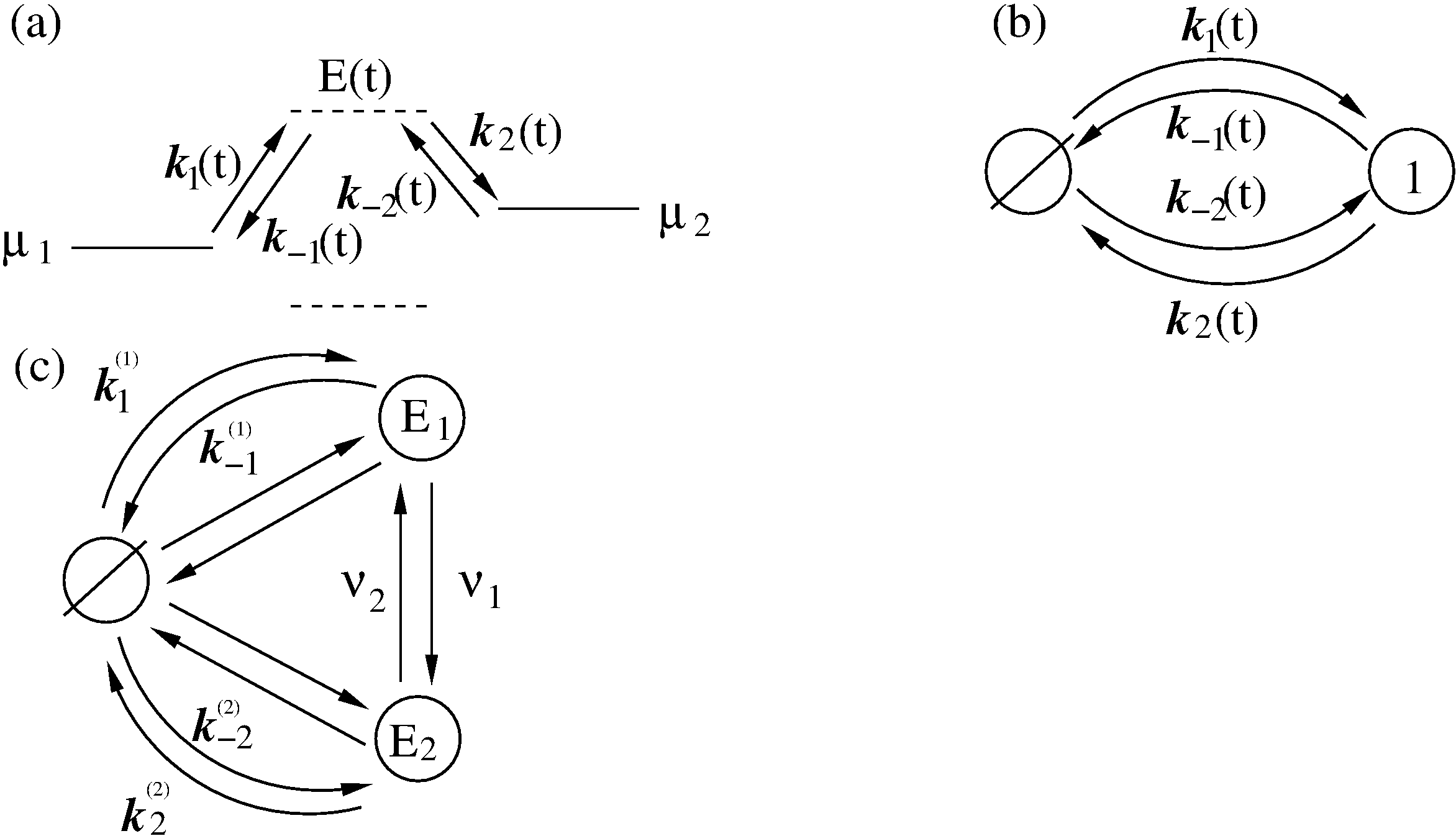
Figure 5: (a) Minimalist model of pump with one time dependent energy level $E(t)$ which can be used to pump particles against a gradient of chemical potential $\Delta\mu$. (b) Corresponding kinetic scheme with time-dependent rates and two states of the pump: empty and filled with one transferred particle. Filling and emptying can occur from either particle reservoirs, $\mu_{1}$ or $\mu_{2}$. (c) Equivalent kinetic scheme corresponding to $E(t)$ having just two realizations with the transition rates $\nu_{1}$ and $\nu_{2}$.

Turning back to adiabatic operation of molecular motors or pumps, we shall analyze now a minimalist model based on time-modulation of the energy levels. The physical background of the idea of adiabatic operation is sound. However, can it be realized in popular models featured by discrete energy levels? The minimalist model contains just one time-dependent energy level $E(t)$ and two constant energy levels corresponding to chemical potentials $\mu_{1}$ and $\mu_{2}$ of two baths of particles between which the transport occurs. They must be considered as electrochemical potentials for charged particles, e.g. Fermi levels of electrons in two leads, or electrochemical potentials of transferred ions in two bath solutions separated by a membrane. Pumping takes place when a time-modulation of $E(t)$ can be used to pump against $\Delta\mu=\mu_{2}-\mu_{1}>0$, see in Fig. 5, (a). Here, both the energy level $E(t)$ and the corresponding rates $k_{1}(t)$ and $k_{-1}(t)$, $k_{2}(t)$ and $k_{-2}(t)$ are time-dependent. Their proper name would be rate constants, if they were time-independent. Given sufficiently slow modulation and fast equilibration at any instant $t$, one can assume local equilibrium condition

$$\frac{k_{1}(t)}{k_{-1}(t)} = \exp\left\{\beta[E(t)-\mu_{1}]\right\},$$

$$\frac{k_{2}(t)}{k_{-2}(t)} = \exp\left\{-\beta[E(t)-\mu_{2}]\right\}\,.$$ (25)

Notice, that this condition is not universally valid. It can be violated by fast fluctuating fields, see in Goychuk and Hänggi (2005) and references cited therein, for a plenty of examples, and an approach beyond this restriction within a quantum-mechanical setting. Rates are generally retarded functionals of energy levels fluctuations and not functions of instant energy levels. However, local equilibrium can be a very good approximation. Fig. 5, (b) rephrases the transport process in Fig. 5, (a) in terms of the states of the pump: empty, state $\emptyset$, and filled with one transferred particle, state $1$. The former state is populated with probability $p_{0}(t)$, and the latter one with probability $p_{1}(t)$, $p_{0}(t)+p_{1}(t)=1$. The empty level can be filled with rate $k_{1}(t)$ from the left bath level $\mu_{1}$, and with rate $k_{-2}(t)$ from the right bath level $\mu_{2}$. The filling flux is thus $j_{f}=(k_{1}+k_{-2})p_{0}$. Moreover, it can be emptied with rate $k_{2}(t)$ to $\mu_{2}$, and with rate $k_{-1}(t)$ to $\mu_{1}$. The corresponding master equations reduce to a single relaxation equation because of probability conservation:

$$\dot{p}_{0}(t) = -[k_{1}(t)+k_{-2}(t)]p_{0}(t)+[k_{2}(t)+k_{-1}(t)]p_{1}(t)$$ (26)

$$= -\Gamma(t)p_{0}(t)+R(t)\;,$$

where

$$\Gamma(t)=k_{1}(t)+k_{-1}(t)+k_{-2}(t)+k_{2}(t)\;,$$ (27)

and

$$R(t)=k_{-1}(t)+k_{2}(t)\;.$$ (28)

The instant flux between the levels $\mu_{1}$ and $E(t)$ is

$$I_{1}(t)=k_{1}(t)p_{0}(t)-k_{-1}(t)p_{1}(t)\;,$$ (29)

and

$$I_{2}(t)=k_{2}(t)p_{1}(t)-k_{-2}(t)p_{0}(t)\;,$$ (30)

between the levels $E(t)$ and $\mu_{2}$. Clearly, the time averages $\bar{I}_{1}=\lim_{t\to\infty}(1/t)\int_{0}^{t}I_{1}(t^{\prime})dt^{\prime}$ and $\bar{I}_{2}=\lim_{t\to\infty}(1/t)\int_{0}^{t}I_{1}(t^{\prime})dt^{\prime}$ must coincide, $\bar{I}_{1}=\bar{I}_{2}=I$, because particles cannot accumulate on the level $E(t)$.

First, we show that pumping is impossible within the approximation of quasi-static rate, i.e. when the rates are considered to be constant at a frozen time instant and one solves the problem within this approximation. Indeed, in this case for a steady-state flux which is instant function of time we obtain:

$$I(t) = \frac{k_{1}(t)k_{2}(t)-k_{-1}(t)k_{-2}(t)}{\Gamma(t)}$$ (31)

$$= \frac{k_{1}(t)k_{2}(t)}{\Gamma(t)}\left[1-e^{\Delta\mu/(k_{B}T)}\right]\;,$$

where in the second line we used (III.1). Clearly for $\Delta\mu>0$, $I(t)<0$ at any $t$. Averaging over time yields,

$$\bar{I}_{qs}=\bar{I}_{f}\left[1-e^{\Delta\mu/(k_{B}T)}\right]\;,$$ (32)

with $\bar{I}_{f}=\lim_{{\cal T}\to\infty}(1/{\cal T})\int_{0}^{\cal T}k_{1}(t)k_{2}(t)dt/\Gamma(t)$. The current flows always from higher $\mu_{2}$ to lower $\mu_{1}$. The same will happen for any number of intermediate levels $E_{i}(t)$ within such an approximation.

III.2 Origin of pumping

One can, however, easily solve Eq. (26) for arbitrary $\Gamma(t)$ and $R(t)$:

$$p_{0}(t)=p_{0}(0)e^{-\int_{0}^{t}\Gamma(t^{\prime})dt^{\prime}}+\int_{0}^{t}dt^{\prime}R(t^{\prime})e^{-\int_{t^{\prime}}^{t}\Gamma(t^{\prime\prime})dt^{\prime\prime}}\;.$$ (33)

The first term vanishes in the limit $t\to\infty$ and a formal expression for steady state averaged flux $\bar{I}$ can be readily written,

$$\bar{I}=\lim_{\cal T\to\infty}\frac{1}{\cal T}\int_{0}^{\cal T}dt[k_{1}(t)+k_{-1}(t)]\int_{0}^{t}dt^{\prime}R(t^{\prime})e^{-\int_{t^{\prime}}^{t}\Gamma(t^{\prime\prime})dt^{\prime\prime}}-\bar{k}_{-1}\;,$$ (34)

where $\bar{k}_{-1}$ is time-averaged $k_{-1}(t)$. However, to evaluate it for some particular protocols of energy and rates modulation is generally a rather cumbersome task. The fact that pumping is possible is easy to understand making the following protocol of energy level and rates modulation: (step 1) energy level $E(t)$ goes down, $E(t)<\mu_{1}$, with an increasing prefactor in $k_{\pm 1}(t)$ (left gate opens), and sharply decreasing prefactor in $k_{\pm 2}(t)$ (right gate is closed), a particle enters pump from the left; (step 2) energy level $E(t)$ goes up, $E(t)>\mu_{2}$, and prefactor in $k_{\pm 1}(t)$ sharply drops, the left gate closes and the right one remains closed; (step 3) the right gate opens and the particle leaves to the right; (step 4) the right gate closes, the energy level $E(t)$ goes down and the left gate opens, so that the initial position in three-dimensional parameter space (two prefactors and one energy level) is repeated, and one cycle is completed. The general idea of ionic pump with two intermittently opening/closing gates has in fact been suggested long time ago Jardetzky (1966).

Some general results can be obtained within this model for adiabatic slow modulation and related to an adiabatic geometric Berry phase $b(t)$, the origin of which can be understood, per analogy with a similar approach used to solve Schroedinger equation in quantum mechanics for adiabatically modulated quasi-stationary energy levels Anandan et al. (1997), by making the following Ansatz to solve Eq. (26): $p_{0}(t)=e^{ib(t)}R(t)/\Gamma(t)+c.c.$. Making a loop in a two-dimensional space of parameters adds or subtracts $2\pi$ to $b(t)$. Furthermore, an additional related contribution, pumping current, appears in addition to one in (32), with averaging done over one cycle period. This additional contribution is proportional to the cycling rate $\omega$, see in Sinitsyn and Nemenman (2007) for detail. However, it is small and cannot override one in (32) consistently with the adiabatic modulation assumptions. Hence, adiabatic pumping against any substantial bias $\Delta\mu>0$ is not possible within this model. This indeed can easily be understood by making a sort of adiabatic approximation in Eq. (33), $\int_{t^{\prime}}^{t}\Gamma(t^{\prime\prime})dt^{\prime\prime}\approx\Gamma(t)(t-t^{\prime})$, and doing an integration by parts therein, so that in the long time limit $p_{0}(t)\approx R(t)/\Gamma(t)+\delta p_{0}(t)$, where $\delta p_{0}(t)\propto\dot{R}(t)\propto\omega$. The first term leads to (32), and the second term corresponds to a small perturbative pump current, which vanishes as $\omega\to 0$. This pump current can be observed only for $\Delta\mu=0$, where $\bar{I}_{qs}=0$. Hence, thermodynamic efficiency of this pump is close to zero in adiabatic pumping regime.

Moreover, for realistic molecular pumps driven e.g. by energy of ATP hydrolysis, the adiabatic modulation is difficult if possible to realize. A sudden modulation of the energy levels, i.e. a power stroke, when the energy levels jump to new discrete positions, is more relevant, especially on a single-molecular level.

III.3 Efficient non-adiabatic pumping

The cases, where $E(t)$ takes on discrete values being a continuous time semi-Markovian process can be handled differently. Especially simple is a particular case with $E(t)$ taking just two values $E_{1}$ and $E_{2}>E_{1}$ with transition rates $\nu_{1}$, and $\nu_{2}$ between those. Then, the transport scheme in Fig. 5, (b) can be rephrased as one in Fig. 5, (c) with rate constants $k_{j}^{(i)}$ for the transitions to and from the energy levels $E_{i}$, $i=1,2$, $j=1,2,-1,-2$, and

$$\frac{k_{1}^{(i)}}{k_{-1}^{(i)}} = \exp\left\{\beta[E_{i}-\mu_{1}]\right\},$$

$$\frac{k_{2}^{(i)}}{k_{-2}^{(i)}} = \exp\left\{-\beta[E_{i}-\mu_{2}]\right\}\,.$$ (35)

Now we have three populations, $p_{0}$ of empty state, $p_{1}$ of level $E_{1}$, and $p_{2}$ of level $E_{2}$. The steady state flux can be calculated as $I=\nu_{1}p_{1}^{(st)}-\nu_{2}p_{2}^{(st)}$, where $p_{1,2}^{(st)}$ are steady state populations. Straightforward, but somewhat lengthy calculations yield

$$I=\frac{\nu_{1}\left(k_{1}^{(1)}+k_{-2}^{(1)}\right)\left(k_{-1}^{(2)}+k_{2}^{(2)}\right)-\nu_{2}\left(k_{1}^{(2)}+k_{-2}^{(2)}\right)\left(k_{-1}^{(1)}+k_{2}^{(1)}\right)}{\sum_{i}k_{i}^{(1)}\sum_{j}k_{j}^{(2)}+\nu_{1}\left(\sum_{j}k_{j}^{(2)}+k_{1}^{(1)}+k_{-2}^{(1)}\right)+\nu_{2}\left(\sum_{j}k_{j}^{(1)}+k_{1}^{(2)}+k_{-2}^{(2)}\right)}\;.$$ (36)

From the structure of this equation it is immediately clear that the flux can be positive for positive $\Delta\mu$ (real pumping), e.g. by considering the limit: $k_{1}^{(1)}\gg k^{(1)}_{-2}$, $k_{-1}^{(2)}\ll k_{2}^{(2)}$, $k_{1}^{(2)}\ll k_{-2}^{(2)}$, $k_{2}^{(1)}\ll k_{-1}^{(1)}$, and $\nu_{1}\gg\nu_{2}$. Physically, it is obvious when $E_{1}<\mu_{1}$, and $E_{2}>\mu_{2}$, together with $k_{1}^{(1)}\gg k_{-2}^{(1)}$ (i.e. the level $E_{1}$ is easily filled from $\mu_{1}$, but not from $\mu_{2}$ because e.g. of a large barrier on the right side – the entrance of pump is practically closed from the right), and $k_{2}^{(2)}\gg k_{-1}^{(2)}$ (i.e. the particle easily goes from $E_{2}$ to $\mu_{2}$ and cannot go back to $\mu_{1}$ because the left entrance is now almost closed). Under these conditions, also $k_{1}^{(2)}\ll k_{-2}^{(2)}$ and $k_{2}^{(1)}\ll k_{-1}^{(1)}$ are well justified. Hence, we obtain for the pumping rate

$$I\approx\frac{\nu_{1}k_{1}^{(1)}k_{2}^{(2)}}{k_{1}^{(1)}k_{2}^{(2)}+\nu_{1}\left(k_{1}^{(1)}+k_{2}^{(2)}\right)}\;.$$ (37)

This expression looks like a standard Michaelis-Menthen rate of enzyme operation, which is customly used in biophysics Nelson (2003) for modeling molecular motors and pumps. Elevation of $E(t)$ level from $E_{1}$ to $E_{2}$ can be effected e.g. by ATP binding in case ionic pumps, with $\nu_{1}\propto c_{ATP}$, where $c_{ATP}$ is ATP concentration. This is a simplest basic model for pumps. From (37) it follows that $I\approx\nu_{1}$ at $\nu_{1}\tau\ll 1$, where $\tau=1/k_{1}^{(1)}+1/k_{2}^{(2)}$ is the sum of filling and emptying times, and it reaches the maximal pumping rate $I_{\rm max}\approx 1/\tau$, for $\nu_{1}\tau\gg 1$. Thermodynamic efficiency of such a pump is $R=\Delta\mu/\Delta E$, where $\Delta E=E_{2}-E_{1}$ is energy invested in pumping. Derivation of approximate Eq. (37) requires that $\exp(\epsilon_{1,2}/k_{B}T)\gg 1$, where $\epsilon_{1}=\mu_{1}-E_{1}$, and $\epsilon_{1}=E_{2}-\mu_{2}$, which is well satisfied already for $\epsilon_{1,2}>2k_{B}T$. Hence $R=\Delta\mu/(\Delta\mu+\epsilon_{1}+\epsilon_{2})$ can be close to one for a large $\Delta\mu\gg\epsilon_{1}+\epsilon_{2}$. Take for example $\Delta E=20\;k_{B}T_{r}\approx 0.5$ eV, which corresponds to a typical energy released by ATP hydrolysis. Then, for $\Delta\mu=0.4$ eV and $\epsilon_{1}=\epsilon_{2}=2k_{B}T_{r}\approx 0.05$ eV, $R=0.8$. Notice that a typical thermodynamic efficiency of Na-K pump is about $R\approx 0.75$. Such a non-adiabatic pumping can thermodynamically be highly efficient indeed with small heat losses. One should remark, however, that the question on whether or not the efficiency at the maximum of power, $P_{W}=I\Delta\mu$, can be larger than one-half or even approach one within this generic model is not that simple. To answer this question, one cannot neglect backward transport, especially when $\Delta\mu$ becomes close to $\Delta E$ ($P_{W}(\Delta\mu=\Delta E)=0$), and one has to specify a concrete model for the rates in the exact result (36). In the case of an electronic pump, like one used by nature in nitrogenase enzymes this can be quantum tunneling rates, see in Goychuk (2006), like Marcus-Levich-Dogonadze rate above. Moreover, imposing intermittently in time a very high barrier either on the left, or on the right can physically correspond to interruption of electron tunneling pathway due to ATP-induced conformational changes, i.e. to modulation of tunnel coupling $V_{\rm tun}(t)$ synchronized with modulation of $E(t)$, as it does occur in nitrogenase. This question of efficiency at maximum power will be analyzed elsewhere else in detail, both for classical and quantum rate models.

To summarize this section, the idea of adiabatic operation of molecular machines is sound. It should be pursued further. However, the known simplest adiabatic pump operates in fact at nearly zero thermodynamical efficiency, while a power stroke mechanism can be highly efficient within the same model. It seems obvious that in order to realize a thermodynamically efficient adiabatic pumping, a gentle operation of molecular machine without erratic jumps, one needs a continuum of states, or possibly many states depending continuously on an external modulation parameter. A further research is thus highly desirable and needed.

IV How can biological molecular motors operate highly efficiently in highly dissipative viscoelastic environments?

As it has been clarified above, Brownian motors can work highly efficiently in dissipative environments causing arbitrary strong viscous friction acting on motor. This corresponds to the case of normal diffusion, $\langle[\delta x(t)]^{2}\rangle=2Dt$, in a force-free case. In a crowded environment of biological cells, diffusion can be, however, anomalously slow, $\langle[\delta x(t)]^{2}\rangle=2D_{\alpha}t^{\alpha}/\Gamma(1+\alpha)$, where $0<\alpha<1$ is power law exponent of subdiffusion, and $D_{\alpha}$ is subdiffusion coefficient Barkai et al. (2012); Höfling and Franosch (2013). There is a huge body of growing experimental evidence for subdiffusion of particles of various sizes, from $2-3$ nm (typical for globular proteins) Guigas et al. (2007); Saxton and Jacobson (1997) to $100-500$ nm Seisenberger et al. (2001); Golding and Cox (2006); Tolic-Norrelykke et al. (2004); Jeon et al. (2011); Parry et al. (2014) (typical for various endosomes), both in living cells, and in crowded polymer and colloidal solutions (complex fluids) physically resembling cytoplasm. There are many theories developed to explain such a behavior Barkai et al. (2012); Höfling and Franosch (2013). One is based on natural viscoelasticity of such complex liquids, see Goychuk (2012c); Waigh (2005) for a review and detail. It has a deep dynamical foundation (see above). Viscoelasticity which leads to above subdiffusion corresponds to a power law memory kernel $\eta(t)=\eta_{\alpha}t^{-\alpha}/\Gamma(1-\alpha)$ in Eqs. (3), (6), where $\eta_{\alpha}$ is fractional friction coefficient, which is related to $D_{\alpha}$ by the generalized Einstein relation, $D_{\alpha}=k_{B}T/\eta_{\alpha}$. Using the notion of fractional Caputo derivative, the dissipative term in Eq. (3) can be abbreviated as $\eta_{\alpha}d^{\alpha}x/dt^{\alpha}$, where the fractional derivative operator $d^{\alpha}f(t)/dt^{\alpha}$ acting on arbitrary function $f(t)$ is just defined by this abbreviation. The corresponding GLE is named fractional Langevin equation (FLE). Its solution yields the above subdiffusion scaling exactly in the inertialess limit, $M\to 0$, corresponding precisely to the fractional Brownian motion Goychuk and Hänggi (2007); Goychuk (2012c), or asymptotically otherwise. The transport in the case of a constant force $f_{0}$ applied is also subdiffusive, $\langle\delta x(t)\rangle=(f_{0}/\eta_{\alpha})t^{\alpha}/\Gamma(1+\alpha)=(f_{0}/(2k_{B}T))\langle[\delta x(t)]^{2}\rangle$. These results correspond exactly to sub-Ohmic model of the spectral density of thermal bath Weiss (1999), $J(\omega)=\eta_{\alpha}\omega^{\alpha}$, within the dynamical approach to generalized Brownian motion. They can be easily understood if to do ad hoc Markovian approximation to the memory kernel, which yields a time-dependent viscous friction, $\eta_{M}(t)\dot{x}(t)$ with $\eta_{M}(t)\propto t^{1-\alpha}$. It diverges, $\eta_{M}(t)\to\infty$, when $t\to\infty$, which leads to subdiffusion and subtransport within this Markovian approximation. Such an approximation can, however, be very misleading in other aspects Goychuk (2015b). Nevertheless, it provokes the question: How can molecular motors, such as kinesin, work very efficiently in such media characterized by virtually infinite friction, interpolating in fact between simple liquids and solids? Important to mention, in any fluid-like environment the effective macroscopic friction, $\eta_{\rm eff}=\int_{0}^{\infty}\eta(t)dt$, must be finite. Hence, a memory cutoff time $\tau_{\rm max}$ must exist, so that $\eta_{\rm eff}\propto\eta_{\alpha}\tau_{\rm max}^{1-\alpha}$. In real life, $\tau_{\rm max}$ can be as large as minutes, or even longer than hours. Hence, on a shorter time scale and on a corresponding spatial mesoscale it is subdiffusion, characterized by $\eta_{\alpha}$, which can physically be relevant indeed and not the macroscopic limit of normal diffusion characterized by $\eta_{\rm eff}$. This observation opens a way for multi-dimensional Markovian embedding of subdiffusive processes with long range memory upon introduction of a finite number $N$ of auxiliary stochastic variables. It is based on a Prony series expansion of power-law memory kernel into a sum of exponentials, $\eta(t)=\sum_{i=1}^{N}k_{i}\exp(-\nu_{i}t)$, with $\nu_{i}=\nu_{0}/b^{i-1}$ and $k_{i}\propto\nu_{i}^{\alpha}$, which can be made very accurate numerically (this is controlled by the scaling parameter $b$), and apart from $\tau_{\rm max}=\tau_{\rm min}b^{N-1}$ possesses also a short cutoff $\tau_{\rm min}=1/\nu_{0}$. The latter one naturally emerges in any condensed medium beyond continuous medium approximation because of real atomistic nature. In numerics, it can be made of the order of time integration step. Hence, it does not matter even within the continuous medium approximation. Even with a moderate $N\sim 10-100$ (number of auxiliary degrees of freedom) Markovian embedding can be done for any realistic time scale of anomalous diffusion with sufficient accuracy Goychuk (2009, 2012c). A very efficient numerical approach based on the corresponding Markovian embedding has been developed for subdiffusion in Refs. Goychuk (2009, 2012c), and for superdiffusion ($\alpha>1$) in Refs. Siegle et al. (2010b, a, 2011). The idea of Markovian embedding is also very natural in view of that any non-Markovian GLE dynamics presents a low-dimensional projection of a hyper-dimensional singular Markovian process described by dynamical equations of motion with random initial conditions. This fact is immediately clear from a well-known dynamical derivation of GLE reproduced above. Somewhat surprising is, however, that not so many $N\sim 10-20$ are normally sufficient in practical applications.

The action of a motor on subdiffusing cargo can be simplistically modeled (a simplest possible theory) by a random force $f(t)$ alternating its direction, when the motor steps on a random network of cytoskeleton Caspi et al. (2002). The driven cargo follows a diffusional process $\langle[\delta x(t)]^{2}\rangle_{t^{\prime}}\propto t^{\beta}$, with some exponent $\beta$, if to make a trajectory averaging of squared displacements $\delta x(t|t^{\prime})=x(t+t^{\prime})-x(t^{\prime})$ over sliding $t^{\prime}$. Within such a modeling $\beta$ clearly cannot exceed $2\alpha$ Bruno et al. (2009), that corresponds to subtransport which alternates its direction in time. Hence, for $\alpha<0.5$ no cargo superdiffusion ($\beta>1$) could not be caused by motors within such a simple approach. However, experiments show Robert et al. (2010); Harrison et al. (2013) that freely subdiffusing cargos (e.g. $\alpha=0.4$ Robert et al. (2010); Bruno et al. (2011)) can superdiffuse , when they are driven by motors also for $\alpha<0.5$ (e.g. $\beta=1.3$ for $\alpha=0.4$ Robert et al. (2010)) ). Hence, a more appropriate modeling of the transport by molecular motors in viscoelastic environments is required. It has been developed quite recently in Refs. Goychuk et al. (2014a, b); Goychuk (2015a), by generalizing pioneering works on subdiffusive rocking Goychuk (2010, 2012c); Goychuk and Kharchenko (2012); Kharchenko and Goychuk (2013); Goychuk and Kharchenko (2013), and flashing Kharchenko and Goychuk (2012) ratchets.

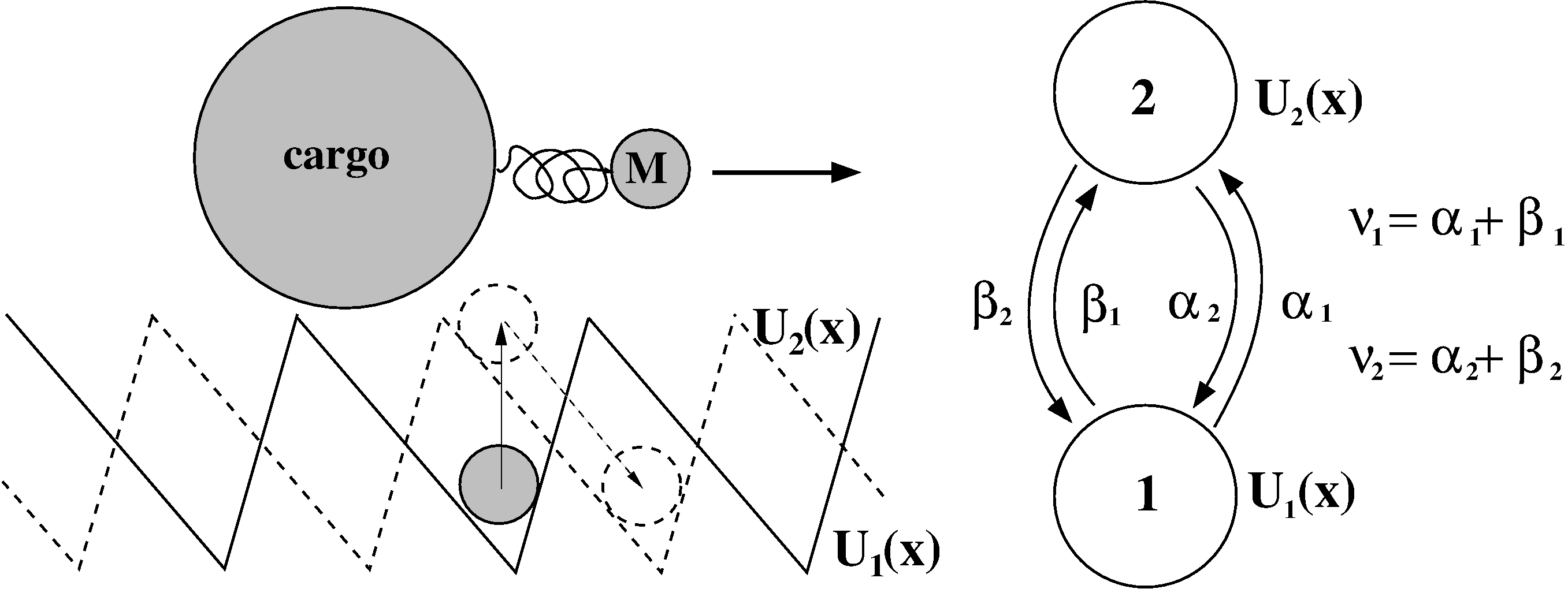
Figure 6: Motor pulling cargo on an elastic linker. The motor can be trapped in a flashing periodic potential (here, two realizations shifted by a half of spatial period are shown). These fluctuations are caused and driven by conformational fluctuations of the motor protein. The minimalist pertinent two-state cyclic model of the corresponding biochemical enzymatic cycle is shown on the right. Mechanical motion, induced by cycling, exerts a back influence on cycling via spatially dependent transition rates. This can cause anomalously slow enzyme kinetics, which cannot be characterized by a turnover rate, in viscoelastic environments Goychuk (2015a).

Viscoelastic effects should by considered on the top of viscous Stokes friction caused by the water component of cytosol. Then, a basic 1d model for a large cargo (20-500 nm) pulled by a much smaller motor (2-10 nm) on an elastic linker, cf. Fig. 6, can be formulated as follows Goychuk (2015a)

$$\eta_{c}\dot{y} = -\int_{0}^{t}\eta(t-t^{\prime})\dot{y}(t^{\prime})dt^{\prime}-\frac{k_{L}(y-x)}{1-(y-x)^{2}/r_{\rm max}^{2}}+\xi_{c}(t)+\xi(t),$$ (38)

$$\eta_{m}\dot{x} = \frac{k_{L}(y-x)}{1-(y-x)^{2}/r_{\rm max}^{2}}-\frac{\partial}{\partial x}U(x,\zeta(t))-f_{L}+\xi_{m}(t).$$ (39)

This presents a generalization of a well-known model of molecular motors Jülicher et al. (1997); Astumian and Bier (1996); Parmeggiani et al. (1999) by coupling motor to a subdiffusing cargo on an elastic linker. Here, both the motor (coordinate $x$) and the cargo (coordinate $y$) are subjected to independent thermal white noises of the environment, $\xi_{m}(t)$, and $\xi_{c}(t)$, respectively, which obey the corresponding FDRs. The both particles are overdamped and characterized by the Stokes frictional forces with frictional constants $\eta_{m}$, and $\eta_{c}$. In addition, on cargo acts viscoelastic frictional force characterized by the memory kernel discussed above (fractional friction model) and the corresponding stochastic thermal force $\xi(t)$ with algebraically decaying correlations. It obeys a corresponding FDR. The motor can pull cargo on an elastic linker with spring constant $k_{L}$ (small extensions) and maximal extension length $r_{\rm max}$ (the so-called finite extension nonlinear elastic (FENE) model Herrchen and Öttinger (1997) is used here). The motor (kinesin) is bound to a microtubule and can move along it in a periodic potential $U(x+L,\zeta(t))=U(x,\zeta(t))$ reflecting microtubule spatial period $L$, and do a useful work against a loading force $f_{L}$ directed against its motion caused by cyclic conformational fluctuations $\zeta(t)$. Microtubule is a polar periodic structure with a periodic but asymmetric distribution of positive and negative charges (overall charge is negative) Baker et al. (2001). Kinesin is also charged and its charge fluctuates upon binding negatively charged ATP molecules and dissociation of the products of ATP hydrolysis. This leads to dependence of the binding potential on the conformational variable $\zeta(t)$. Given two identical heads of kinesin, the minimalist model is to assume that there are only two conformational states of the motor (this is a gross oversimplification, of course) with $U_{1,2}(x):=U(x,\zeta_{1,2})$, and $U_{1}(x+L/2)=U_{2}(x)$ as an additional symmetry condition, so that a half-step $L/2$ is associated with conformational fluctuations $1\to 2$, or $2\to 1$. During one cycle $1\to 2\to 1$ in the forward direction with the rates $\alpha_{1}(x)$ and $\beta_{2}(x)$, one ATP molecule is hydrolyzed, whereas if this cycle is reverted in the backward direction with the rates $\beta_{1}(x)$ and $\alpha_{2}(x)$, see Fig. 6, one ATP molecule is synthesized. The dependence of chemical transition rates on the position $x$ through the potential $U_{1,2}(x)$ reflects a two way mechano-chemical coupling. It it is capable to incorporate allosteric effects which indeed can be very important for optimal operation of molecular machines Cheng et al. (2015). Such effects can possibly emerge, for example, because the probability of binding of ATP molecule (substrate) to kinesin motor or release of products can be influenced by electrostatic potential of the microtubule. In the language of Ref. Cheng et al. (2015) this corresponds to an information ratchet mechanism to distinguish it from the energy ratchet where the rates of potential switches do not depend on the motor states (no feedback) and are fixed. Such an allostery can be used to create highly efficient molecular machines Cheng et al. (2015). In accordance with general principles of nonequilibrium thermodynamics applied to cyclic kinetics Hill (1989)

$$\frac{\alpha_{1}(x)\beta_{2}(x)}{\alpha_{2}(x)\beta_{1}(x)}=\exp[|\Delta\mu_{\rm ATP}|/(k_{B}T)],$$ (40)

for any $x$, where $|\Delta\mu_{\rm ATP}|$ is the free energy released in ATP hydrolysis and used to drive one complete cycle in forward direction. It can be satisfied, e.g., by choosing

$$\frac{\alpha_{1}(x)}{\alpha_{2}(x)} = \exp[(U_{1}(x)-U_{2}(x)+|\Delta\mu_{\rm ATP}|/2)/(k_{B}T)],$$

$$\frac{\beta_{1}(x)}{\beta_{2}(x)} = \exp[(U_{1}(x)-U_{2}(x)-|\Delta\mu_{\rm ATP}|/2)/(k_{B}T)].$$ (41)

The total rates

$$\nu_{1}(x)=\alpha_{1}(x)+\beta_{1}(x),$$

$$\nu_{2}(x)=\alpha_{2}(x)+\beta_{2}(x)$$ (42)

of the transitions between two energy profiles must satisfy

$$\frac{\nu_{1}(x)}{\nu_{2}(x)}=\exp[(U_{1}(x)-U_{2}(x))/(k_{B}T)]$$ (43)

at thermal equilibrium. This is condition of the thermal detailed balance, where the dissipative fluxes vanish both in the transport direction and within the conformational space of motor, at the same time Jülicher et al. (1997); Astumian and Bier (1996). It is obviously satisfied for $|\Delta\mu_{\rm ATP}|\to 0$. Furthermore, on symmetry grounds, not only $\alpha_{1,2}(x+L)=\alpha_{1,2}(x)$, $\beta_{1,2}(x+L)=\beta_{1,2}(x)$, but also, $\alpha_{1}(x+L/2)=\beta_{2}(x)$ and $\alpha_{2}(x+L/2)=\beta_{1}(x)$. It should be emphasized that such linear motors as kinesin I or II work only one way: they utilize chemical energy of ATP hydrolysis for doing mechanical work. They cannot operate in reverse on average, i.e. to use mechanical work in order to produce ATP in a long run, even if a two way mechano-chemical coupling can provide such an opportunity in principle. This is very different from such rotary motors as F0F1-ATPase which is completely reversible and can operate in two opposite directions. Allosteric effects can also play a role to provide such a directional asymmetry in the case of kinesin motors. Allostery should be considered as generally important for a proper design of various motors best suited for different tasks.

For kinesins, neither cargo nor external force $f_{L}$ should explicitly influence the chemical rate dependencies on the mechanical coordinate $x$. This leaves still some freedom in use of different models of rates. One possible choice is Goychuk (2015a)

$$\nu_{1}(x) = \alpha_{1}(x)+\alpha_{1}(x+L/2)\exp[-(U_{2}(x)-U_{1}(x)+|\Delta\mu_{\rm ATP}|/2)/(k_{B}T)],$$

$$\nu_{2}(x) = \alpha_{1}(x)\exp[-(U_{1}(x)-U_{2}(x)+|\Delta\mu_{\rm ATP}|/2)/(k_{B}T)]+\alpha_{1}(x+L/2)\;,$$ (44)

with $\alpha_{1}(x)=\alpha_{1}$ within some $\pm\delta/2$ neighborhood of the minimum of potential $U_{1}(x)$ and zero otherwise. Correspondingly, the rate $\beta_{2}(x)=\alpha_{1}$ within $\pm\delta/2$ neighborhood of the minimum of potential $U_{2}(x)$. The rationale behind this choice is that these rates correspond to lump reactions of ATP binding and hydrolysis, and if to choose the amplitude of the binding potential to be about $|\Delta\mu_{\rm ATP}|$, and a sufficiently large $\delta$, the rates $\nu_{1,2}(x)$ can be made almost independent of the position of motor along microtubule Goychuk (2015a), considering allosteric effects to be almost negligible in this particular respect. This allows to compare this model featured by bidirectional mechano-chemical coupling with a corresponding flashing energy ratchet model, where the switching rates between two potential realizations are spatially-independent constants, $\nu_{1}=\nu_{2}=\alpha_{1}$. The latter model has been developed in Ref. Goychuk et al. (2014b). Notice that even for reversible F1-ATPase motors such an energy ratchet model can provide very reasonable and experimentally relevant results Perez-Carrasco and Sancho (2010). Moreover, if the linker is very rigid, $k_{L}\to\infty$, one can exclude the dynamics of cargo and to consider one compound particle with a renormalized Stokes friction and the same algebraically decaying memory kernel and moves subdiffusively in a flashing potential. Such an anomalous diffusion molecular motor model has been proposed and investigated in Ref. Goychuk et al. (2014a). The main results of Goychuk et al. (2014a), which were confirmed and further generalized in Goychuk et al. (2014b); Goychuk (2015a), create the following emerging coherent picture of molecular motors pulling subdiffusing (when free) cargos in viscoelastic environment of living cells. First, if normally diffusing (when free) motor is coupled to subdiffusing cargo it will be eventually enslaved by the cargo and also subdiffuse Goychuk et al. (2014b). However, when the motor is bounded to microtubule, it can be guided by the binding potential fluctuations, which are eventually induced by its own cyclic conformation dynamics driven by the free energy released in ATP hydrolysis. It slides towards a new potential minimum after each potential change, or can fluctuationally escape to another minimum, see Fig. 6 to realize this. Large binding potential amplitude $U_{0}\gg k_{B}T$ (should exceed $10-12\,k_{B}T$, see Fig. 6 and a corresponding discussion in Goychuk et al. (2014b) to understand why) makes the motor strong. For a large $U_{0}$ the probability to escape is small, and the motor will typically slide down to a new minimum and its mechanical motion along microtubule will be completely synchronized with potential flashes and conformational cycles. It steps then (stochastically but unidirectionally) to the right in Fig. 6 with mean velocity ${\rm v}=L\alpha_{1}/2$. In such a way, using a power stroke like mechanism a strong motor like kinesin II (with stalling force $F\sim 6-8$ pN) can completely beat subdiffusion and transport very efficiently even subdiffusing (when free) cargos. This requires, however, that flashing occurs slower than relaxation. The larger the cargo the larger is also the fractional friction coefficient $\eta_{\alpha}$, and slower relaxation. The relaxation is algebraically slow. However, it can be sufficiently fast in absolute terms on the time scale $1/\alpha_{1}$, so that mechanism is realized for sufficiently small cargos. The results of Goychuk et al. (2014a, b); Goychuk (2015a) indicate that smaller cargos, $20-100$ nm, will typically be transported by strong kinesin motors quite normally, $\langle y(t)\rangle\sim\langle x(t)\rangle\propto t^{\alpha_{\rm eff}}$, with $\alpha_{\rm eff}=1$, at typical motor turnover frequencies $\nu=\alpha_{1}/2\sim 1-200$ Hz, provided that $f_{L}=0$. This already explains why the diffusional exponent $\beta\sim 2\alpha_{\rm eff}$ can be larger than $2\alpha$. However, for larger cargos, $100-300$ nm, larger turnover frequencies and when the motor works in addition against a constant loading force $f_{L}$, anomalous transport regime emerges with $\alpha\leq\alpha_{\rm eff}\leq 1$. Clearly, when $f_{L}$ approaches the stalling force $F$ the transport becomes anomalous. The effective transport exponent $\alpha_{\rm eff}$ is thus essentially determined by binding potential strength, motor operating frequency, cargo size, and loading force, apart from $\alpha$.

It is very surprising that thermodynamics efficiency of such a transport can be very high even within anomalous transport regime. This result is not trivial at all. Indeed, the useful work done by motor in anomalous regime against loading force $f_{L}$, scales sublinearly in time, $W(t)=f_{L}\langle x(t)\rangle\propto t^{\alpha_{\rm eff}}$ Goychuk and Kharchenko (2013); Kharchenko and Goychuk (2013); Goychuk et al. (2014a). However, the free energy transformed into directional motion scales generally as $E_{\rm in}(t)\propto t^{\gamma}$, where $0<\gamma\leq 1$. $\gamma=1$ for rocking, or flashing ratchets driven by either periodic force, or random two state force, or by random fluctuations of potential characterized by a well-defined mean turnover rate $\nu=\nu_{1}\nu_{2}/(\nu_{1}+\nu_{2})$. Then, $E_{\rm in}(t)\propto\nu t$. In the energy balance, the rest, $E_{\rm in}(t)-W(t)$, is dissipated as a net heat $Q(t)$ transferred to the environment. Thermodynamic efficiency is thus Goychuk (2015a)

$$R(t)=W(t)/E_{\rm in}(t)\propto 1/t^{\lambda}$$ (45)

where $\lambda=\gamma-\alpha_{\rm eff}$. Hence, for $R(t)\propto 1/t^{1-\alpha_{\rm eff}}$ for $\gamma=1$. It declines algebraically in time, like also does the mean power $P_{W}(t)=W(t)/t\propto 1/t^{1-\alpha_{\rm eff}}$. However, temporally, for a typical time required to relocate a cargo within a cell it can be very high, especially when $\alpha_{\rm eff}$ is close to one. Even more interesting occurs in the case of bidirectional mechano-chemical coupling, because the biochemical cycling rates $\nu_{1,2}(x)$ in this case can strongly depend on mechanical motion for a sufficiently large $U_{0}$, when allosteric effects start to play a very profound role. Indeed, if available $|\Delta\mu_{\rm ATP}|$ becomes smaller than the sum of energies required to enhance the potential energy of motor by two potential flashes (see vertical arrow in Fig. 6) during two halves of one cycle, then the enzyme cycling in its conformational space will not generally stop. It can, however, start to occur anomalously slow with a power exponent $\gamma<1$. The average number of forward enzyme turnovers occurring with consumption of ATP molecules scales then as $\langle N(t)\rangle\propto t^{\gamma}$ in time, and $E_{\rm in}(t)=|\Delta\mu_{\rm ATP}|\langle N(t)\rangle\propto t^{\gamma}$. This indeed happens within the model we consider here, see in Goychuk (2015a) for a particular example with $U_{0}=30\;k_{B}T_{r}\approx 0.75\;eV$, $|\Delta\mu_{\rm ATP}|=20\;k_{B}T_{r}\approx 0.5\;eV$, where $\gamma\approx 0.62$ and $\alpha_{\rm eff}\approx 0.556$ at the optimal load $f_{L}\approx 8.5$ pN, when the motor pulls a large cargo at the same time. Thermodynamic efficiency declines in this case very slowly, with $\lambda\approx 0.067$, so that $R(t)$ is still about 70% (!) at the end point of simulations corresponding to physical 3 seconds. Such a high efficiency is very surprising and should provide one more lesson for our intuition that should finally learn and recognize the power of FDT on nanoscale. For microscopic and nanoscopic motion occurring at thermal equilibrium the energy lost in frictional processes is regained from thermal random forces. Therefore, heat losses can, in principle, be small even for an anomalously strong dissipation. This is the reason why the attempts to reduce friction on nanoscale are misguided. They can, pretty counter-intuitively, even hamper efficiency, down to zero as the so-called dissipationless Brownian (pseudo)-motors reveal. One should think differently.

The efficiency at maximum power can also be high in the normal transport operating regime within the discussed model. Indeed, for $U_{0}=30\;k_{B}T_{r}$ and smaller cargo in Goychuk (2015a), the transport remains almost normal until the maximum of efficiency $R$ is reached at about 80% for an optimal $f_{L}^{\rm(max)}\sim 9$ pN (see Fig. 8 in Goychuk (2015a), where $f_{0}$ corresponds to $f_{L}$ here). The nearly linear dependence of the efficiency on load therein until it reaches about 70% indicates that the motor steps with almost the same maximal velocity as at zero loading force $f_{L}$. The following simple heuristic considerations can be used to rationalize the numerical results. The motor develops a maximal driving force $F$, which depends on $U_{0}$, the motor turnover rate, and temperature (via an entropic contribution), see Fig. 6 in Goychuk et al. (2014b), where $F=f_{0}^{stall}$. It is the stalling force. The larger $U_{0}$, the stronger is the motor and larger $F$. Let us assume that the motor stepping velocity declines from ${\rm v}_{0}$ to zero with increasing loading force $f_{L}$ as ${\rm v}(f_{L})={\rm v}_{0}[1-(f_{L}/F)^{a}]$, where $a\geq 1$ is a power law exponent. Within the linear minimalist model of motor considered above, and also in an inefficient transport regime within the considered model, $a=1$, i.e. the motor velocity declines linearly with load. However, in a highly efficient nonlinear regime this dependence is strongly nonlinear, $a\gg 1$. The maximum of the motor power $P_{W}(f_{L})=f_{L}{\rm v}(f_{L})$ is reached at $f_{L}^{\rm(max)}=F/(1+a)^{1/a}$, with ${\rm v}(f_{L}^{\rm(max)})=a{\rm v}_{0}/(1+a)$. For $a=1$, $f_{L}^{\rm(max)}=F/2$ and the dependence $P_{W}(f_{L})$ is parabolic. With the increase of $U_{0}$, $a$ is also strongly increased and the dependence $P_{W}(f_{L})$ becomes strongly skewed, in agreement with numerics. Since the input motor power $P_{\rm in}$ does not depend on load within our model in the energy ratchet regimes, the motor efficiency $R=P_{W}/P_{\rm in}$ just reflects one of $P_{W}$. Hence, the maximum of $R$ versus $f_{L}$ does correspond to the maximum efficiency at maximum power and can exceed $1/2$. The same heuristic considerations can be applied to the results presented in Ref. Parmeggiani et al. (1999) for very efficient normal motors. Of course, these results are not necessarily experimentally relevant for e.g. known kinesin I motors whose maximal efficiency is about 50% Nelson (2003). However, our theory can be very relevant for devising artificial motors having other tasks because it provides a biophysically very reasonable model where efficiency at maximum power can be larger than the Jacobi bound of linear stochastic dynamics. It must be stressed, however, that in anomalous transport regime one cannot define power and one should introduce the notion of sub-power Goychuk and Kharchenko (2013); Kharchenko and Goychuk (2013).

One should remark also the following. Even at $f_{L}=0$, when thermodynamic efficiency is formally zero, $R(t)=0$, something useful is yet done: the cargo is transferred on a certain distance by overcoming the dissipative resistance of the environment. However, neither potential energy of motor, nor one of cargo is increased. This is actually normal modus operandi of linear molecular motors like kinesins I or II, very differently from ionic pumps whose the primary goal is to increase the (electro)chemical potential of transferred ions, i.e. to charge a battery. Such a $R=0$ regime, should, however, be contrasted with zero efficiency of frictionless rocking pseudo-ratchets. In our case, the useful work is done against environment. Pseudo-ratchets are not capable to do any useful work in principle.

V Conclusions

In this contribution we reviewed some main operating principles of miniscule Brownian machines operating on nano- and microscales. Unlike in macroscopic machines, thermal fluctuations and noise do play profound and moreover very constructive role in microworld. In fact, thermal noise plays a role of stochastic lubricant which supplies energy to the Brownian machines to compensate for their frictional losses. This is the very essence of fluctuation-dissipation theorem that the both processes, i.e. frictional losses and energy gain from the thermal noise are completely compensated on average at thermal equilibrium. Classically, thermal noise vanishes at absolute zero of temperature (which physically cannot be achieved anyway, in accordance with the third law of thermodynamics), and then only friction would win (classically). However, quantum noise (vacuum zero-point fluctuations) is present even at the absolute zero of temperature. Therefore, friction cannot win also at the absolute zero, and quantum Brownian motion never stops. These fundamental facts allow, in principle, for a complete transformation of the driver energy into a useful work by isothermal Brownian engines. Their thermodynamic efficiency approaches unity, when the net heat losses vanish. This happens when the motor operates most closely to thermal equilibrium. And this can be done at any, arbitrarily strong dissipation and ambient temperatures. No need to go into a deep quantum cold or to strive for a high quality quantum coherence. A most striking example for this is provided by the high transport and thermodynamic efficiency of molecular motors in subdiffusive transport regime. Operating anomalously slow, in mathematical terms, i.e. exhibiting sublinear dependences of both the transport distance and the number of motor turnovers on time, such motors can be pretty fast in the absolute terms and work under a heavy load, see in Goychuk (2015a). In this and also other aspects, the intuitive understanding of subdiffusion and subtransport as extremally slow can be very misleading, see in Goychuk (2012a, b); Goychuk and Kharchenko (2014). On the other hand, the frictionless rocking pseudo-ratchets cannot do any useful work, as we clarified in this review.

Scientifically sound possibility to approach the theoretical maximum of thermodynamic efficiency of isothermal motors at arbitrarily strong dissipation and ambient temperatures is intrinsically related to a possibility of reversible dissipative classical computing without heat production. However, such an adiabatic operation would be infinitesimally slow. Clearly, nobody needs neither such a motor, nor computer. Moreover, adiabatic operation of dissipative pumps involving discrete energy levels is possible only for a vanishing load. Here, a natural question emerges: What is thermodynamic efficiency at maximum power? The linear dynamics result that $R_{\rm max}=1/2$ presents a theoretical upper bound is, however, generally completely wrong within nonlinear stochastic dynamics, as we showed in this review with three (!) examples. This opens a door for design of highly efficient Brownian and molecular motors. Moreover, the recent model results in Goychuk (2015a) for a normal transport of sufficiently small subdiffusing (when free) cargos by a kinesin motor with a very high thermodynamical efficiency at optimal external load do imply that thermodynamical efficiency at maximum power within that model can also be well above 50%. The earlier results for a normal diffusion molecular motors within a model of a very similar kind Jülicher et al. (1997); Astumian and Bier (1996) obtained in Parmeggiani et al. (1999) also corroborate such conclusions. Such models are able to mimic allosteric interactions within minimalist model setups. Chemical allosteric interactions, which are intrinsically highly nonlinear, can optimize performance of various molecular motors. This line of reasoning is especially important for design of artificial molecular motors Cheng et al. (2015). It should be pursued further. Quantum effects can also be important to arrive at this goal, even when quantum coherence does not play any role, i.e. on the level of rate dynamics with quantum rates (like in Pauli master equation). In particular, it has been shown in this review within a simplest toy model possible that quantum effects (related to inverted regime of quantum particle transfer) can lead to thermodynamic efficiencies at maximal power larger than one half for the machine operating both in direct and reverse directions. Quantum coherence can also play here a role, which should be clarified in further research. Undoubtedly, quantum coherence is central for quantum computing, which is obviously reversible Feynman (1996). However, this is a different story.

I hope that the readers of this review will find it most useful in, especially, liberating themselves and possibly others from some common fallacies, both spoken and unspoken which unfortunately pervaded literature and hinder the further progress. A valid coherent picture emerges.