An Asynchronous Implementation of
the Limited Memory CMA-ES

Abstract

We present our asynchronous implementation of the LM-CMA-ES algorithm, which is a modern evolution strategy for solving complex large-scale continuous optimization problems. Our implementation brings the best results when the number of cores is relatively high and the computational complexity of the fitness function is also high. The experiments with benchmark functions show that it is able to overcome its origin on the Sphere function, reaches certain thresholds faster on the Rosenbrock and Ellipsoid function, and surprisingly performs much better than the original version on the Rastrigin function.

I Introduction

Evolutionary algorithms are a nice tool for solving complex optimization problems for which no efficient algorithms are currently known. They belong to black-box optimization algorithms, i.e. the algorithms which learn the problem instance they solve by querying the function value, or “fitness”, of a solution from that instance. In their design, evolutionary algorithms rely on the ideas which are rooted in natural evolution: problem solutions “mutate” (undergo small changes), “mate” or “cross over” (new solutions are created from parts of other solutions), undergo “selection” (only a part of solutions proceeds to the next iteration).

One of the most prominent features of evolutionary algorithms is the high degree of parallelism. Most evolutionary algorithms, such as genetic algorithms, evaluate hundreds of solutions in parallel, which allows efficient usage of multicore and distributed computer systems. However, many such algorithms are generational, that is, they must have many solutions to be completely evaluated before taking further actions. If the time of a single solution evaluation may differ from time to time, such evaluation scheme may be quite inefficient, because many threads finish their work too early and wait for long periods of time until the next work pieces become available. To overcome this problem, steady-state evolutionary algorithms are developed, which do not have the notion of generations, so they have a potential to become asynchronous and to use computer resources in a better way.

Optimization problems are often subdivided into three groups: discrete problems, continuous problems and mixed problems. Among them, continuous problems received significant attention in classical mathematical analysis, so a rich body of methods was developed which makes optimization efficient by using information about gradient and second derivatives. Black-box algorithms for solving continuous optimization problems, while remaining in the black-box setting (i.e. using only the function value, but not gradient, which may not exist at all), borrowed many ideas from classic methods. One of the most famous algorithms of this sort is the Broyden-Fletcher-Goldfarb-Shanno algorithm, or simply BFGS [1]. Modern evolution strategies, e.g. evolutionary algorithms for continuous optimization which tend to self-adapt to the problem’s properties, also follow this direction, which led to the appearance of the evolution strategy with covariance matrix adaptation (CMA-ES [2]).

The CMA-ES algorithm, as follows from its name, learns a covariance matrix which encodes dependencies between decision variables, together with some more traditional parameters like the step size. This algorithm shows very good convergence at many problems, including non-separable, multimodal and noisy problems. However, it comes with a drawback, which is high computational complexity ($O(n^{2})$ per function evaluation, where $n$ is the problem size, and $O(n^{2})$ memory for storing the covariance matrix). An attempt to reduce memory requirements and decrease the running time using numeric methods for Cholesky factorization was recently done in [3]. Several modifications were developed, including sep-CMA-ES [4], which gives linear time and space complexity, but at the cost of worse performance on non-separable functions. However, most if not all algorithms from this family, while being generational by their nature, have a cost of maintaining the algorithm state after evaluation of the generation which is comparable to or even higher than a single function evaluation. This makes it nearly impractical to use them in multicore or distributed computing environments, especially when function evaluation is cheap.

The only attempt to turn an evolution strategy from the CMA-ES family into an asynchronous algorithm, which is known to authors, belongs to Tobias Glasmachers [5]. This work, however, addresses a so-called natural evolution strategy [6], which is much easier to make asynchronous due to properties of updates used in this algorithm. This approach can not be easily extended on other flavours of CMA-ES.

This paper presents our current research results on making asynchronous a more typical CMA algorithm, proposed by Ilya Loshchilov [7] and called “limited memory CMA-ES” (LM-CMA-ES). This algorithm is designed to work with large scale optimization problems (with the number of dimensions $n\geq 1000$) which are not solvable with the usual CMA-ES. The key idea which made this possible is to compute the approximation of the product of a square root of the covariance matrix by a random vector sampled from the Gaussian distribution, which is a way CMA-ES samples new individuals, by an iterative process which references only $m$ vectors, $m\ll n$, from the past evaluations. The step sizes are restored in a similar way. This makes it possible to avoid storing the covariance matrix or its parts explicitly (which takes $O(n^{2})$ memory) and finding its eigenpairs (which takes $O(n^{3})$ time per generation). In the same time, this method does not sacrifice rotation symmetry in the way the sep-CMA-ES does.

The main idea of this paper is to change the algorithm which updates the stored data in order to make it incremental, which turns the LM-CMA-ES algorithm into a steady-state one. After this change, the solutions can be evaluated asynchronously, which makes the overall implementation asynchronous. The results of the very early experimentation stage are presented in our previous paper [8]. Compared to that paper, we use more evaluation functions, more algorithm configurations, measure much more data (not only CPU load) and perform a comparison to the original LM-CMA-ES algorithm.

#1

The rest of the paper is structured as follows. Section II contains the description of our asynchronous modification of the LM-CMA-ES. Section III sets up the research questions which are solved in the paper. Section IV describes the methodology used in experiment design, the experiment setup, results and their discussion. Section V concludes.

II Algorithm Description

In this section we describe the proposed asynchronous modification of the LM-CMA-ES algorithm. Section II-A briefly describes the original LM-CMA-ES algorithm as in [7], and Section II-B explains the modifications which we made.

II-A The Original LM-CMA-ES

The key idea of the LM-CMA-ES algorithm is to implicitly restore the covariance matrix $C$ from $m\ll n$ selected vector pairs $(v^{(t)},p_{c}^{(t)})$ sampled at some past moments of time. Each vector pair consists of $v^{(t)}$, the solution represented in the coordinate system based on eigenvectors of the covariance matrix $C^{(t)}$ corresponding to the moment of time $t$, and the evolution path $p_{c}^{(t)}$ represented in the same coordinate system.

The algorithm itself does not need the entire matrix by itself, but only its left Cholesky factor $A$ (such that $C=A\times A^{T}$) and its inverse $A^{-1}$. Generally they also require $\Theta(n^{2})$ space to be stored, but if we know that the matrix $C$ is constructed from only $m$ pairs of vectors, we can use these vectors to simulate an effect of $A\times x$ and $A^{-1}\times x$ for an arbitrary vector $x$. The total time needed to do this is $O(nm)$ per single function evaluation.

This algorithm, as any algorithm belonging to the CMA-ES family, has a number of parameters, such as $\lambda$, the number of sampled solutions per iteration, $\mu$, the number of best solutions which are used to construct the next reference search point, weights $w_{i}$ for creation of this search point, and a number of other parameters. However, they all have default values, which were shown to be efficient for optimization of multiple benchmark functions [7].

II-B Our Modifications

Our implementation is different from the LM-CMA-ES algorithm in the following key aspects:

• We do not use generations of size $\lambda$. Instead, we use several threads which work independently most of the time. First, a thread samples a solution based on the reference search point, the implicit Cholesky factor $A$ and using generator of random numbers from the normal distribution $\mathcal{N}(0,1)$. Then it evaluates this solution using the fitness function. After that, the thread enters a critical section, performs update operations, makes copies of the necessary data and leaves the critical section.

• Due to the one-at-a-time semantics of an update, the modification no longer belongs to the $(\mu/\mu_{w},\lambda)$ scheme, but rather can be described as $(m+1)$ – the algorithm maintains $m$ best solution vectors and updates this collection when a new solution comes. This may have some drawbacks on complex functions, as the algorithm has a larger probability to converge to a local optimum, but the simpler update scheme introduces smaller computational costs inside a critical section, which improves running times.

III Research Questions

How can we compare the quality of different algorithms, given a single problem to solve? There are many measures which assist researchers in doing this. Probably the most three popular measures, especially when one considers multiple cores in use, are the following ones:

1. The best possible solution quality. The main aim of this measure is to determine how good the considered algorithm is in determining the problem’s features, and which fitness function values it is able to reach. To track this value, one can run the algorithm until it finds an optimum within the given precision (for example, $10^{-10}$), or until a sufficiently big computational budget is spent (for example, $10^{6}$ fitness function evaluations), or until one can show that the algorithm cannot find a better solution in a reasonable time.

2. The best solution quality under a certain wall-clock time limit. This is quite a “practical” measure widely used in solving real-world problems. However it suffers a drawback: one cannot really compare the results of different algorithms without any problem knowledge. For example, a difference of $0.1$ in the fitness values can be really big for some problems and negligibly small for some other problems.

3. The wall-clock time to obtain a solution of the given quality. This is a more “theoretical” measure because the computational budget is not limited, and it is often a known optimum value which is taken to be a threshold. However we may expect a better scaling of results achieved in this way, which depends less on the problem’s properties.

In this paper, we compare our asynchronous modification of the LM-CMA-ES algorithm with the original generational implementation of the same algorithm on different benchmark problems. As these problems have varying difficulty for these algorithms, it is unrealistic to create the uniform experiment setups for all these problems. So we drop the second measure and consider only the first one (the best possible solution quality) and the third one (the wall-clock time to obtain a solution of the given quality). Based on these comparisons, we try to find answers for the following questions:

1. Are the considered algorithms able to solve the problems to optimality (i.e. within the precision of $10^{-10}$)? Which problems are tractable by which algorithms?

2. What are the convergence properties of the algorithms? How the changes introduced in the asynchronous version affect the convergence?

3. How the performance of the algorithms depends on the number of cores?

4. How the performance of the algorithms depends on the computational complexity of the fitness function?

5. Which are the problems where the asynchronous version is better, and where is it worse?

IV Experiments

This section explains the methodology used while designing the experiments (Section IV-A), shows the setup of the experiments, including technical details (Section IV-B), presents and explains the results of the preliminary experiments (Section IV-C), and ends with the main experiment results and their discussion (Section IV-D).

IV-A Methodology

When one configures an experiment, one has to choose one of the possible values for several parameters. We consider the following important parameters:

1. The problem type (the type of the function to be optimized),

2. The problem dimension (the number of decision variables).

3. The computational complexity of the problem (the computational effort required to evaluate a single solution, probably as a function of the problem dimension and the fitness value).

4. The number of CPU cores used to run the algorithm.

All these parameters, except for the third one, have been considered in the literature before. The third parameter (the computational complexity) typically was considered as a function of the problem dimension and the fitness value which is determined exclusively by the problem type. Due to the fourth research question, we decided to treat separately the computational complexity because this gives a chance to adjust the ratio of fitness time to update time, which influences the overall CPU utilization, without influencing other problem characteristics. One can expect that, for example, as the fitness function becomes more and more “heavy”, while all other parameters are left unchanged, the CPU utilization becomes better.

IV-B Setup

We used the following benchmark functions for the first experiment parameter:

• the Sphere function: $f(x)=\sum_{i=1}^{n}{x_{i}^{2}}$;

• the Rastrigin function:
  $f(x)=10n+\sum_{i=1}^{n}{\left(x_{i}^{2}-10\cos(2\pi x_{i})\right)}$;

• the Rosenbrock function:
  $f(x)=\sum_{i=1}^{n-1}\left(100\left(x_{i+1}-x_{i}^{2}\right)^{2}+(1-x_{i})^{2}\right)$;

• the Ellipsoid function: $f(x)=\sum_{i=1}^{n}{\left(\sum_{j=1}^{i}{x_{j}}\right)^{2}}$.

For the second experiment parameter (the problem’s dimension), we use the values 100, 300 and 1000.

For the third experiment parameter (the computational complexity of a fitness function), we either use the fitness function as it is, or augment it with a procedure which changes nothing in the fitness function result but introduces additional computation complexity. This additional complexity is achieved by running the Bellman-Ford algorithm on a randomly generated graph with 10 000 edges and 200, 400, or 600 vertices. This produces the linear growth of the additional complexity, which is similar to or exceeds the “natural” computational complexity of the fitness function.

For the fourth experiment parameter (the number of cores), we use the values 2, 4, 6, and 8.

There were three termination criteria, which stop the algorithm under the following conditions:

1. The function value is close to the optimum with the absolute precision of $10^{-10}$. The optimum values of all the considered functions are known to be zeros.

2. The number of fitness function evaluations exceeds $10^{6}$.

3. For the asynchronous implementation, the value of the parameter $\sigma$ becomes less than $10^{-20}$, which reflects the algorithm’s stagnation in the current point.

Each experiment configuration was run for 100 times for configurations without additional computational complexity and for 50 times otherwise.

For monitoring the overall performance, both in terms of convergence and of using multiple cores, we track the median values of the wall-clock running time needed to reach a certain threshold $t$, and the median values of the processor’s cores load for the time from the beginning of the run until the threshold $t$. For each problem we have to choose several values of the threshold $t$, which we do by analysing the preliminary experiments.

IV-C Preliminary Experiments and Their Results

The preliminary experiments were designed to get preliminary answers to the first two research questions, and also to find suitable fitness function thresholds for each fitness function we used. We did several trial runs of the asynchronous implementation of the LM-CMA-ES algorithm with the problem dimension of 100 without additional computation complexity and with different numbers of available cores.

Figure 1: Example fitness function plots on Sphere

Figure 2: Example fitness function plots on Rastrigin

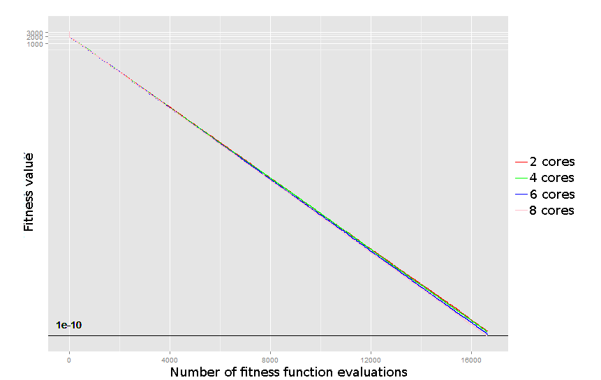
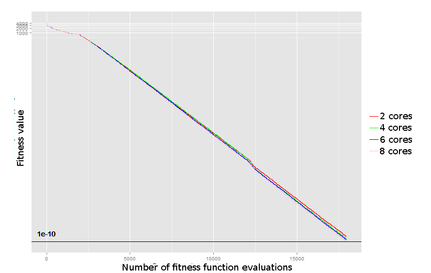
Fig. 1 and 2 show that the Sphere and Rastrigin functions are typically optimized to the global optimum independently of the number of cores (in other words, the algorithm always finds a point with the fitness value less than $10^{-10}$). One can notice the linear convergence in the case of these two functions. For the Rastrigin function there is one linear piece with a smaller slope in the beginning, which seems to correspond to the search for the surroundings of the global optimum. For these two functions the logarithmically equidistant thresholds seem to be the optimal choice, so we select the values of $1$, $3\cdot 10^{-2}$, $10^{-5}$, $3\cdot 10^{-7}$, $10^{-10}$.

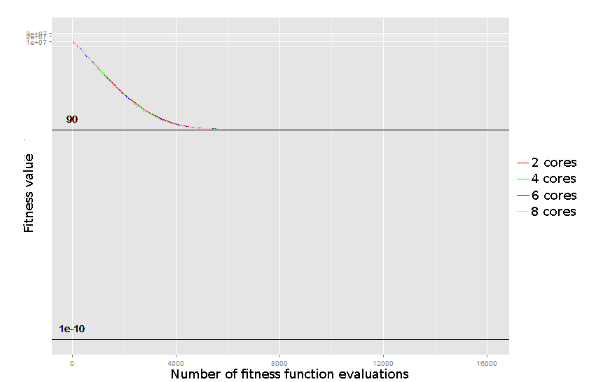
On Fig. 3 one can see a different kind of convergence for the Rosenbrock function. This function is quite difficult for the asynchronous algorithm, as all the runs converge to approximately 90 and then stop having any progress. This is a characteristic trait of this function, as the optimizers typically reach the valley first and then try to find an optimum within the valley using a very small gradient. For this function we take as a threshold the value of 100, which is close enough to the stagnation point, and the value of 3000, which should be reachable by any sensible optimizer. We also include the value $10^{-10}$ from the termination criterion and two intermediate values of $10^{-2}$ and $10^{-6}$.

Figure 3: Example fitness function plots on Rosenbrock

Figure 4: Example fitness function plots on Ellipsoid

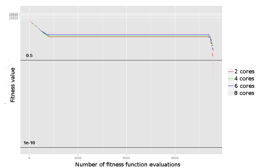
Finally, Fig. 4 shows a similar but slightly different kind of convergence for the Ellipsoid function. In this case, unlike Rosenbrock, after a large number of fitness function evaluations the algorithm is sometimes able to learn a new gradient and find the optimum. This can follow from the 1/5-th rule used in the algorithm, which is not very efficient in this problem. For the threshold values, we took the same values as for the Rosenbrock function.

IV-D Main Experiment Results and Discussion

#1

For the Sphere function (Table LABEL:main-sphere), one can see that both algorithms reach the optimum of this problem. The worst behavior of the proposed algorithm can be seen when the number of cores is high (e.g. 8) and the fitness function complexity is low. This corresponds to the case where the most time is spent on waiting for a critical section. The best behavior is demonstrated when the number of cores is high and the fitness function complexity is also high. Under these conditions, the proposed algorithm, while using an update rule which is generally worse, reaches the optimum faster due to more efficient usage of multiple cores.

For the Rastrigin function (Table LABEL:main-rastrigin), the proposed algorithm always finds an optimum, but the original LM-CMA-ES never does that, which was surprising. This change can be attributed to the update rule as well, but in this case a simpler rule brings better results.

The Rosenbrock (Table LABEL:main-rosenbrock) and the Ellipsoid (Table LABEL:main-ellipsoid) functions are particularly hard for both algorithms. The proposed algorithm typically produces worse results, but in the case of high computational complexity of the fitness function it reaches the thresholds faster. This can be attributed both to the update rule (which seems to be too greedy for these problems) and to the efficient usage of multiple cores.

V Conclusion

We presented our first attempt to implement an asynchronous version of the LM-CMA-ES algorithm. Our algorithm is the best when the number of cores is high and the computation complexity of the fitness function is also high. It uses a different update rule than the LM-CMA-ES algorithm which generally is not very good, however, the efficient usage of multiple cores compensates for this fact on the Sphere benchmark function, and brings to some fitness functions thresholds faster on the Rosenbrock and the Ellipsoid function. A surprising fact is that it performs on the Rastrigin problem much better than the original algorithm.

#1 This work was partially financially supported by the Government of Russian Federation, Grant 074-U01.

References

- [1] D. F. Shanno, “Conditioning of quasi-Newton methods for function minimization,” Mathematics of Computation, vol. 24, no. 111, pp. 647–656, 1970.
- [2] N. Hansen, S. D. Müller, and P. Koumoutsakos, “Reducing the Time Complexity of the Derandomized Evolution Strategy with Covariance Matrix Adaptation (CMA-ES),” Evolutionary Computation, vol. 11, no. 1, pp. 1–18, 2003.
- [3] O. Krause and C. Igel, “A more efficient rank-one covariance matrix update for evolution strategies,” in Proceedings of Foundations of Genetic Algorithms XIII, 2015, pp. 129–136.
- [4] R. Ros and N. Hansen, “A Simple Modification in CMA-ES Achieving Linear Time and Space Complexity,” in Parallel Problem Solving from Nature X, ser. Lecture Notes in Computer Science. Springer, 2008, no. 5199, pp. 296–305.
- [5] T. Glasmachers, “A Natural Evolution Strategy with Asynchronous Strategy Updates,” in Proceeding of Genetic and Evolutionary Computation Conference. ACM, 2013, pp. 431–437.
- [6] D. Wierstra, T. Schaul, T. Glasmachers, Y. Sun, J. Peters, and J. Schmidhuber, “Natural evolution strategies,” Journal of Machine Learning Research, vol. 15, pp. 949–980, 2014.
- [7] I. Loshchilov, “A Computationally Efficient Limited Memory CMA-ES for Large Scale Optimization,” in Proceeding of Genetic and Evolutionary Computation Conference. ACM, 2014, pp. 397–404.
- [8] V. Arkhipov and M. Buzdalov, “An asynchronous implementation of the limited memory CMA-ES: First results,” in Proceedings of International Conference on Soft Computing MENDEL, 2015, pp. 37–40.