Abstract

A method is suggested for treating the well-known deficiency in the use of Padé approximants that are well suited for approximating rational functions, but confront problems in approximating irrational functions. We develop the approach of self-similarly corrected Padé approximants, making it possible to essentially increase the class of functions treated by these approximants. The method works well even in those cases, where the standard Padé approximants are not applicable, resulting in divergent sequences. Numerical convergence of our method is demonstrated by several physical examples.

PACS numbers: 02.30.Lt (Sequences, series, and summability); 02.30.Mv (Approximations and expansions); 02.90.+p (Other topics in mathematical methods in physics)

1 Introduction

In many branches of physics and applied mathematics, there exists the standard problem, when a sought function is given as an expansion in powers of an asymptotically small variable, but it is necessary to define this function in the domain of finite, or large, or even infinite values of the variable. Then some extrapolation techniques are required.

Probably, the simplest and the most often used method of extrapolation is by means of Padé approximants. An approximant $P_{n/m}(x)$ is the ratio of two polynomials $P_{n}(x)$ and $P_{m}(x)$ of the order $n$ and $m$, respectively. The coefficients of the Padé approximant are defined trough the coefficients of the given power series [1, 2], from the requirement of the asymptotic equivalence to the given series of the sought function $f(x)$.

Padé approximants locally are the best rational approximations of power series. Their poles determine singular points of the approximated functions [1, 2]. Calculations with Padé approximants are straightforward and can be performed with $Mathematica^{\textsuperscript{\textregistered}}$.

From the emerging sequences of approximants, one has to select those that are holomorphic functions. Not all approximants generated by the procedure are holomorphic. The holomorphy of diagonal Padé approximants in a given domain implies their uniform convergence inside this domain [3].

However, the use of the Padé approximants confronts the well known indeterminate problem, when these approximants are not applicable. The meaning of this problem is as follows.

Suppose we are considering a non-negative function with the asymptotic behavior at infinity $f(x)\simeq Ax^{s}$, with a known critical index $s$ and a given expansion at small $x$,

$$f(x)=a_{0}+\sum_{n=1}^{N}a_{n}x^{n}+O(x^{N+1})\;.$$ (1)

Here $N$ is an integer and $N\geqslant 1$. The standard suggestion for the solution of the problem of reconstructing the amplitude $A$, is based on the following [4, 5].

Suppose we need to calculate the critical amplitude $A$. To this end, let us apply a transformation of the original series $f(x)$, so that to obtain the transformed series $T(x)=f(x)^{-1/s}$, in order to get rid of the $x^{s}$ behavior at infinity. Applying the technique of diagonal Padé approximants in terms of $xT_{n/(n+1)}(x)$, one can readily obtain the sequence of approximations ${A_{n}}$ for the critical amplitude $A$ as

$$A_{n}=\lim_{x\to\infty}(xT_{n/(n+1)}(x))^{-s}\;.$$ (2)

Of course, not always Padé approximants are convergent. The uniform convergence of diagonal sequences of Padé approximants has been established, e.g., for the Stieltjes-Markov-Hamburger series [1, 6]. The Stieltjes moment problem can possess a unique solution or multiple solutions. The latter is called the indeterminate problem. The existence of a unique solution or multiple solutions depends on the behavior of the moments. This is in contrast to the problem of moments for a finite interval [7], which is uniquely defined, if the solution exists [8]. The original work of Stieltjes has been clearly explained in [9, 10].

From the theory of $S$-fractions one deduces a divergence by oscillations of Padé approximants in the indeterminate case [8]. The phenomenon of spurious poles, when approximants can have poles which are not related to the underlying function, can also lead to divergence of the Padé sequence [1, 6, 8].

Generally, the form of the solution in the indeterminate case is covered by the Nevanlinna theorem, expressing non-negative functions through a mixture of rational and non-rational contributions[7, 11, 12, 13]. The former can be interpreted as the part covered by four entire functions related to the construction of Padé approximants, while the latter is only a non-rational function from the Nevanlinna-class [14]. Thus, in the indeterminate case, Padé approximants are not sufficient. Below, we suggest an approximation scheme which can express the irrational part explicitly and describes the rational part with Padé approximants.

In the present paper, we consider approximations for single-valued real functions, because of which we keep in mind the standard Padé approximants. We will not consider complex multivalued functions, or sets of functions, which are all given as Taylor series around the same point, when we would need to find a simultaneous rational approximation to such a vector of several functions, when it would be possible to employ the Padé - Hermite approximation [1, 15] yielding the so-called algebraic approximants [1, 15, 16]. Note that, instead of considering simultaneously a set of functions, it is admissible to treat each of them separately.

2 Self-similarly corrected Padé approximants

The main idea of the method we suggest is to separate out an initial approximation that could treat the irrational part of the sought function, so that the higher approximations, constructed above the initial approximation, could be represented by Padé approximants. The form of the initial approximation can be chosen by resorting to self-similar approximation theory [17, 18] resulting in root approximants [19, 20] or factor approximants [21, 22].

Assume that we start with a self-similar approximation $K(x)$, ensuring the correct critical index $s$, while all other additional parameters are to be obtained by asymptotically matching the approximant with the truncated series for $f(x)$. As a starting approximation $K(x)$, we can employ iterated root approximants [19, 20] or factor approximants [21, 22]. Then the initial approximation for the amplitude is

$$A_{0}=\lim_{x\to\infty}(K(x)x^{-s})\;.$$

To define the higher-order approximations, we can resort to the method of corrected approximants [19, 20]. For this purpose, to find out corrections to the critical amplitude, we divide the original series (1) for $f(x)$ by $K(x)$, and denote the new series as

$$G(x)=\frac{f(x)}{K(x)}\;.$$

Assuming that the irrational part has already been included in $K(x)$, we now can invoke rational approximants. Thus, we finally construct a sequence of diagonal Padé approximants asymptotically equivalent to $G(x)$, so that the approximate amplitudes are expressed by the formula

$$A_{n}=A_{0}\lim_{x\to\infty}[G_{n/n}(x)]\;.$$ (3)

The role of the starting approximation $K(x)$ is crucial. It is supposed not only to approximate the irrational part of the sought function, but also to ensure the convergence of Padé approximants for the rational part.

The starting approximation can be viewed as a control function, constructed so that to ensure the convergence of the sequence of corrected Padé approximants, even if the standard Padé scheme diverges. Our the most important suggestion is not only in promoting the idea of controlled Padé sequences, but also in conjecturing that the control function should be chosen among the low-parametric subset of irrational self-similar approximants.

In the examples to be treated below, we assume that the critical index at infinity is available. This information, as is known, makes it possible to improve the accuracy of approximants [4, 20, 23, 24].

When only a single ”critical index” $s$ is known in advance, we are limited to the iterated roots and factor approximants, noting that self-similar approximants can be uniquely defined. In all examples studied below, the control function is indeed found easily. More general self-similar roots and continued roots [25, 26, 27], can be applied to more general situations, when, in addition to $s$, more detailed corrections to the leading scaling behavior are available.

Note that Padé approximants by themselves cannot serve as control functions, since the standard Padé scheme cannot be controlled [28, 29]. It is also useful to mention that the suggested approach can be generalized to the case of complex functions, for which self-similar approximation theory is applicable, with the use of complex control functions [23]. However, here we limit ourselves by single-valued real functions.

In this way, the corrected approximants are applicable in all cases, including those where the standard Padé approximants diverge. On the other hand, when the standard scheme is convergent, the corrected scheme also converges, exhibiting either the similar behavior of approximants, or often accelerating convergence. These cases are illustrated in the following sections.

Let us emphasize that our main aim in the present paper is to extend the applicability of Padé approximants. Of course, we could employ one of the variants of self-similar approximation theory [17, 18, 19, 20, 21, 22, 25, 26] for the whole problem, not invoking Padé approximants at all. However, the techniques of Padé approximants are well developed and there are standard programs for defining their coefficients. It would therefore be tempting to slightly modify the method of Padé approximants in order to be able to resort to the standard techniques of calculating their coefficients, at the same time extending their applicability to the cases where the standard Padé approximants are not applicable. Such an extension is a principal novelty of the present paper, not considered in our previous publications.

3 Self-similar roots as control functions

Choosing an irrational part $K(x)$, playing the role of a control function, it is convenient to invoke the self-similar root approximants [19, 20, 27], which we shall employ below. To make this paper self-consistent, we briefly delineate the way of defining the self-similar root approximants. A more detailed description can be found in the earlier publications [19, 20, 27].

Suppose, the sought function $f(x)$ is given as an expansion in powers of a small variable $x\rightarrow 0$, so that the $k$-th order series reads as

$$f_{k}(x)=f_{0}(x)\left(1+\sum_{n=1}^{k}a_{n}x^{n}\right)\;,$$ (4)

where

$$f_{0}(x)=Ax^{\alpha}\qquad(A\neq 0)$$ (5)

is a known zero-order term. And assume that we need to extrapolate this series to the region of finite variables, including the limit of the large variable, where the sought function behaves as

$$f(x)\simeq Bx^{s}\qquad(x\rightarrow\infty),$$ (6)

with an unknown amplitude $B$. Then the $k$-th order self-similar root approximate $R_{k}^{*}(x)$ is given [19, 20, 27] by the formula

$$\frac{R_{k}^{*}(x)}{f_{0}(x)}=\left(\left(\ldots(1+A_{1}x)^{n_{1}}+A_{2}x^{2}\right)^{n_{2}}+\ldots+A_{k}x^{k}\right)^{n_{k}}\;,$$ (7)

in which the first $k-1$ powers are

$$n_{j}=\frac{j+1}{j}\qquad(j=1,2,\ldots,k-1)\;,$$ (8)

while the power $n_{k}$ is

$$n_{k}=\frac{s-\alpha}{k}\qquad(k=1,2,\ldots)\;.$$ (9)

Here all parameters $A_{i}$ are uniquely defined by the accuracy-through-order procedure, that is, by expanding this root approximant in powers of $x$ and equating the similar terms of this expansion and of series (4).

The root approximant (7) at large variables behaves as

$$R_{k}^{*}(x)\simeq B_{k}x^{s}\qquad(x\rightarrow\infty)\;,$$ (10)

with the amplitude

$$B_{k}=A\left(\left(\ldots(A_{1}^{2}+A_{2})^{3/2}+A_{3}\right)^{4/3}+\ldots+A_{k}\right)^{(s-\alpha)/k}\;.$$ (11)

In order to separate the irrational part of the sought function, it is sufficient to employ a low-order root approximant, usually, accepting that of second order. Below, we illustrate the method by several examples. First, we consider rather simple functions, for which exact forms are known, and respectively, for which the accuracy of the method can be explicitly estimated. Then we treat more complicated cases related to interesting physical problems.

4 Convergence and accelerated convergence

4.1 Convergence: Mittag-Leffler function

Consider the Mittag-Leffler function appearing in fractional evolution processes [30],

$$F(x)=\rm{erfc}(x)\exp\left(x^{2}\right)\;.$$ (12)

For small $x$ in the lowest orders, one has

$$F(x)\simeq 1-\frac{2x}{\sqrt{\pi}}+x^{2}-\frac{4x^{3}}{3\sqrt{\pi}}+\frac{x^{4}}{2}+O(x^{5})\;,$$ (13)

and for large $x$,

$$F(x)\simeq Ax^{-1}\qquad(x\rightarrow\infty)\;,$$

where $A=1/\sqrt{\pi}$

Let us take as a control function the second-order self-similar root approximant

$$K(x)=R_{2}^{*}(x)=\left[\left(\frac{2x}{\sqrt{\pi}}+1\right)^{2}-\frac{2(\pi-4)x^{2}}{\pi}\right]^{-1/2}\;.$$ (14)

There is no significant difference in the behavior of approximations for the amplitude $A$ for both schemes of applying Padé approximants. Good convergence is achieved as is shown in Fig. 1.

Figure 1: Percentage errors for the large-variable amplitude of the Mittag-Leffler function, with the increasing approximation order $n$: the errors for the corrected Padé approximants are shown with circles, and for the standard Padé scheme, with squares.

4.2 Accelerated convergence: quartic oscillator

Let us consider the dimensionless ground state energy $e(g)$ of the quantum one-dimensional quartic anharmonic oscillator [31]. Here $g$ stands for the dimensionless coupling constant. The asymptotic expansion of $e(g)$ in the weak-coupling limit, when $g\rightarrow 0$, is

$$e(g)\simeq a_{0}+a_{1}g+a_{2}g^{2}+...+a_{18}g^{18}+...\;,$$ (15)

where a few starting coefficients are

$$a_{0}=\frac{1}{2},\quad a_{1}=\frac{3}{4},\quad a_{2}=-\frac{21}{8},\quad a_{3}=\frac{333}{16},\quad a_{4}=-\frac{30885}{128}\;.$$

At a large coupling parameter $g\rightarrow\infty$, the ground-state energy $e(g)$ diverges as $Ag^{1/3}$, with $A=0.667986$.

Applying the standard Padé approximants, one obtains the amplitudes

$$A_{2}=0.759147,\quad A_{3}=0.734081,\quad A_{4}=0.720699,\quad A_{5}=0.712286,$$

$$A_{6}=0.706466,\quad A_{7}=0.702176,\quad A_{8}=0.698869,\quad A_{9}=0.696173\;.$$

The last approximant of the sequence has the error of $4.21967\%$.

The control function for the method of corrected Padé approximants is the second-order iterated root,

$$K(g)=R_{2}^{*}(g)=\frac{1}{2}\left(\left(\frac{9g}{2}+1\right)^{2}-18g^{2}\right)^{1/6}\;,$$ (16)

yielding $A_{0}=0.572357$.

The results of calculations, according to the corrected Padé approximants methodology, are as follows:

$$A_{1}=A_{2}=A_{0},\quad A_{3}=0.587104,\quad A_{4}=0.63279,\quad A_{5}=0.655086,$$

$$A_{6}=0.660334,\quad A_{7}=0.661945,\quad A_{8}=0.663225,\quad A_{9}=0.665346\;.$$

The last approximant of the sequence gives an error of only $-0.3952\%$, by the order of magnitude better than the standard approach.

5 Treating divergence by oscillations

5.1 Correlation function

In the course of calculating temporal correlation functions [32], one often meets the functions of the following structure

$$f(x)=\sqrt{x^{2}+4}-x\;.$$ (17)

At small $x$, the expansion is

$$f(x)\simeq 2-x+\frac{x^{2}}{4}-\frac{x^{4}}{64}+O(x^{6})\;.$$ (18)

For large $x$, the following asymptotic behavior holds:

$$f(x)\simeq 2x^{-1}+O(x^{-3})\;.$$ (19)

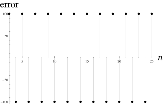
Applying the standard Padé scheme brings a divergent by oscillation solution for the amplitude, bounded by the values $0$ and $4$, as is shown in Fig. 2.

Figure 2: Percentage errors for the amplitude, with increasing approximation order, obtained with Padé approximants for function (17).

But employing the corrected scheme with the control function

$$K(x)=R_{2}^{*}(x)=\frac{2}{\sqrt{x^{2}/2+x+1}}$$ (20)

leads to a convergent result for the amplitude, as is shown in Fig. 3.

Figure 3: Percentage errors for the amplitude, with increasing approximation order, obtained with the corrected Padé approximants for function (17).

5.2 Debye-Hukel function

The correlation function of the Gaussian polymer [33], is given in the closed form as

$$f(x)=\frac{2}{x}-\frac{2(1-\exp(-x))}{x^{2}}\;.$$ (21)

For small $x$, we have

$$f(x)\simeq 1-\frac{x}{3}+\frac{x^{2}}{12}-\frac{x^{3}}{60}+\frac{x^{4}}{360}+O(x^{5})\;,$$ (22)

and for large $x$,

$$f(x)\simeq 2x^{-1}\qquad(x\rightarrow\infty)\;.$$

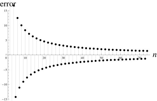
The standard Padé scheme gives oscillating solutions with the magnitude of oscillations slowly decreasing with the approximation order, as is shown in Fig. 4.

Figure 4: Debye-Hukel function. Percentage errors for the amplitude, with increasing approximation order, obtained with the standard Padé approximants.

.

The method of corrected Padé approximants, with a rather simple control function,

$$K(x)=R_{2}^{*}(x)=\frac{\sqrt{6}}{\sqrt{x^{2}+4x+6}}\;,$$ (23)

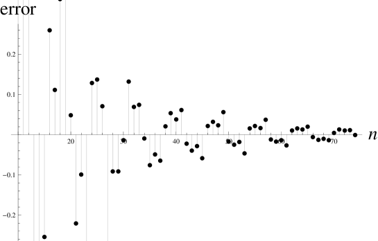
demonstrates very good results improving convergence, as is shown in Fig. 5.

Figure 5: Debye-Hukel function. Percentage errors for the amplitude, with increasing approximation order, obtained with the corrected approximants.

5.3 Branched polymer

The structure factor of a three-dimensional branched polymer is given by the confluent hypergeometric function [34, 35]

$$S(x)=F_{1}(1;\frac{3}{2};\frac{3}{2}x)\;,$$ (24)

where $x$ is a dimensionless wave-vector modulus. At small $x$ (long-waves) the coefficients in the expansion are given by the general expression

$$a_{n}=\left(-\frac{3}{2}\right)^{n}\Gamma(n+1)\;{\displaystyle/}\;\frac{\Gamma(1)\left[n!\Gamma\left(n+\frac{3}{2}\right)\right]}{\Gamma\left(\frac{3}{2}\right)}\;,$$ (25)

while for large $x$ (short-waves), one has

$$S(x)\simeq\frac{1}{3}\;x^{-1}\;.$$

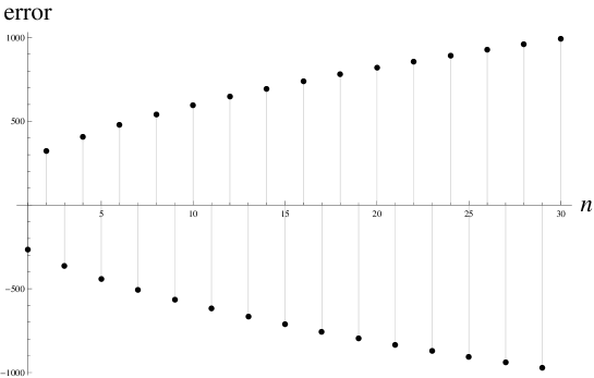
The standard Padé scheme gives divergent oscillating results for the amplitude, with an increasing magnitude for larger orders, as demonstrated in Fig. 6.

Figure 6: Branched polymer. Percentage errors for the amplitude, with increasing approximation order, obtained with Padé approximants.

The control function $K(x)$ in this case can be taken as the factor approximant

$$K(x)=f_{3}^{*}(x)=(1+(0.142857\,-0.255551i)x)^{-0.5-1.67705i}\times$$

$$\times(1+(0.142857\,+0.255551i)x)^{-0.5+1.67705i}\;.$$ (26)

The corrected Padé approximants demonstrate very good convergence, as is seen in Fig. 7.

Figure 7: Branched polymer. Percentage errors for the amplitude, with increasing approximation order, obtained with the corrected Padé approximants.

6 Treating convergence to wrong values

It may happen that the standard Padé method seems to converge very fast, however to a wrong value. This case can be viewed as divergent by oscillations, where the oscillations occur between this wrong value and $\infty$.

6.1 Particle in a box

In the calculation of the ground-state energy of a quantum particle in a one-dimensional box [36], one meets the following function

$$f(g)=\frac{\pi^{2}}{128}\left(\frac{1}{2}+\frac{16}{\pi^{4}g^{2}}+\frac{1}{2}\sqrt{1+\frac{64}{\pi^{4}g^{2}}}\right)\;.$$ (27)

At small $g\rightarrow 0$, this function possesses the expansion

$$f(g)\simeq\frac{1}{8\pi^{2}g^{2}}\sum_{n=0}a_{n}g^{n}\;,$$ (28)

with

$$a_{0}=1,\quad a_{1}=\frac{\pi^{2}}{4},\quad a_{2}=\frac{\pi^{4}}{32},\quad a_{3}=\frac{\pi^{6}}{512},\quad a_{4}=0,\quad a_{5}=-\frac{\pi^{10}}{131072},\quad a_{6}=0,\ldots$$

We shall be interested in finding the limiting value $f(\infty)$ in the asymptotic expression

$$f(g)\simeq f(\infty)\left(1+O\left(g^{-2}\right)\right),\quad\left(g\rightarrow\infty\right)\;,$$ (29)

whose exact limit is $0.077106$.

For convenience, instead of the original function (27), we consider the expression $8\pi^{2}g^{2}\times f(g)$. The standard Padé scheme fails, converging very fast, already at $n=2$, to the wrong value $0.0385531$, or producing rapid oscillations between this values $0.0385531$ and $\infty$, with varying the approximation order.

The control function for the method of corrected Padé approximants can be taken as the third-order iterated root approximant

$$K(g)=R_{3}^{*}(g)=\left(\frac{3\pi^{6}g^{3}}{1024}+\left(\frac{\pi^{4}g^{2}}{64}+\left(\frac{\pi^{2}g}{8}+1\right)^{2}\right)^{3/2}\right)^{2/3}\;.$$ (30)

A very good convergence is achieved in the method of corrected Padé approximants, as is shown in Fig. 8.

Figure 8: Particle in a box. Percentage errors for the amplitude, with increasing approximation order, for corrected Padé approximants.

6.2 Generating function

The following function

$$f(x)=\left(\sqrt{x^{2}+1}+x\right)^{a}\;,$$ (31)

with an arbitrary $a$, is used as a touch-stone generating function [37] for the sequence of numbers $a_{n}$ corresponding to the coefficients in the expansion of (31) at small $x$, with

$$a_{n}=\frac{2^{n}\left(\frac{a}{2}-\frac{n}{2}+1\right)^{\bar{n}}}{n!\left(\frac{n}{a}+1\right)}\;,$$ (32)

while for large $x$,

$$f(x)\simeq 2^{a}x^{a}\qquad(x\rightarrow\infty)\;.$$

Here $m^{\bar{k}}$ means $m(m+1)\ldots(k+m-1)$.

For concreteness, let us consider the case of $a=1/3$. Note that the function needed for constructing the standard scheme, that is,

$$T(x)\simeq 1-x+\frac{x^{2}}{2}-\frac{x^{4}}{8}+O(x^{6})\;,$$

misses the powers of $x$ required for getting the correct large-variable limit. Therefore the value of the amplitude, predicted already at the first step $A_{1}=1$, does not change with $n$. Formally, the calculated amplitude oscillates between $1$ and $\infty$.

On the contrary, the corrected scheme works well, with the control function

$$K(x)=R_{2}^{*}(x)=\sqrt[6]{x^{2}+(x+1)^{2}}\;,$$ (33)

as is illustrated in Fig. 9.

Figure 9: Generating function. Percentage errors for the amplitude, with increasing approximation order, obtained with the corrected approximants, corresponding to the control function (33).

7 Treating strongly divergent solutions

7.1 Hard-core scattering problem

Let us illustrate the method for the problem considered by Baker and Gammel [4]. When calculating the scattering length of a repulsive square-well potential, one meets the integral

$$S(x)=\int_{0}^{x}\left(\frac{\sin t}{t^{3}}\;-\;\frac{\cos t}{t^{2}}\right)\;dt\;,$$ (34)

whose limit $S(\infty)=\pi/15$. Baker and Gammel state that the Taylor series expansion of this integral cannot be treated by the standard Padé techniques, but require some more general methods. We show below that this integral can be effectively treated by means of the corrected approximants using the self-similar root approximants.

The small-variable expansion of this integral reads as

$$S(x)\simeq\frac{x}{9}-\frac{x^{3}}{135}+\frac{x^{5}}{2625}-\frac{4x^{7}}{297675}+\frac{2x^{9}}{5893965}+O(x^{11})\;.$$ (35)

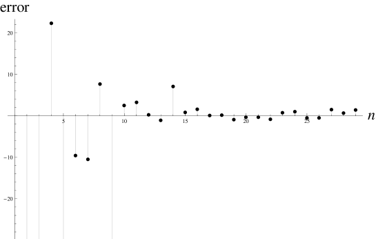
The results of the standard Padé scheme are meaninglessly divergent, as is illustrated in Fig.10.

Figure 10: Scattering problem. Percentage errors for the amplitude, with increasing approximation order, obtained with the standard Padé approximants.

It turns out that the sequence of the iterated roots gives the most stable results. The technique of iterated roots is very easy to apply, which yields [19, 20] the following few first terms,

$$R_{1}^{*}(x)=\frac{x}{9\sqrt{\frac{2x^{2}}{15}+1}}\;,$$

$$R_{2}^{*}(x)=\frac{x}{9\sqrt[4]{\frac{34x^{4}}{2625}+\left(\frac{2x^{2}}{15}+1\right)^{2}}}\;,$$

$$R_{3}^{*}(x)=\frac{x}{9\sqrt[6]{\frac{152x^{6}}{55125}+\left(\frac{34x^{4}}{2625}+\left(\frac{2x^{2}}{15}+1\right)^{2}\right)^{3/2}}}\;,...,$$ (36)

which can be extended to an arbitrary order.

Employing the corrected scheme, with the simplest root approximant $R^{*}_{1}(x)$ as a control function, we get the following sequence of approximations for $S(\infty)$:

$$S_{1}=0.30429,\quad S_{2}=0.247712,\quad S_{3}=0.238538,\quad S_{4}=0.238538,\quad S_{5}=0.232624,$$

$$S_{6}=0.228707,\quad S_{7}=0.225813,\quad S_{8}=0.223642,\quad S_{9}=0.221929,\quad S_{10}=0.220562,$$

$$S_{11}=0.219428,\quad S_{12}=0.218486,\quad S_{13}=0.217682,\quad S_{14}=0.216994,\quad S_{15}=0.216394,$$

$$S_{16}=0.21587,\quad S_{17}=0.215405,\quad S_{18}=0.214992,\quad S_{19}=0.214621,\quad S_{20}=0.214287,$$

$$S_{21}=0.213984,\quad S_{22}=0.213709,\quad S_{23}=0.213457,\quad S_{24}=0.213226,\quad S_{25}=0.213013\;.$$

The error of the last approximant equals $1.70644\%$.

7.2 Wilson Loop

The $N=4$ super Yang - Mills circular Wilson loop [38] is given by the following expression,

$$f(y)=\frac{2\exp\left(-\sqrt{y}\right)I_{1}\left(\sqrt{y}\right)}{\sqrt{y}}\;,$$ (37)

where $I_{1}$ is a modified Bessel function of the first kind. Let us set $\sqrt{y}=x$. For small $x$, we have

$$f(x)\simeq 1-x+\frac{5x^{2}}{8}-\frac{7x^{3}}{24}+\frac{7x^{4}}{64}+O(x^{5})\;,$$ (38)

and at large $x$, one has

$$f(x)\simeq\sqrt{\frac{2}{\pi}}x^{-3/2}\qquad(x\rightarrow\infty)\;.$$

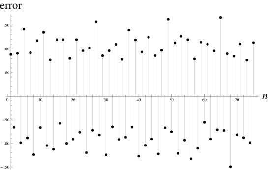
Applying the standard scheme leads to divergent results, as is clearly seen in Fig. 11.

Figure 11: Wilson loop. Percentage errors for the amplitude, with increasing approximation order, obtained with the standard Padé approximants.

Employing the control function

$$K(x)=R_{2}^{*}(x)=\left(\frac{5x^{2}}{18}+\left(\frac{2x}{3}+1\right)^{2}\right)^{-3/4}$$ (39)

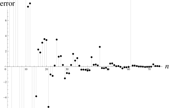
and constructing the corrected Padé approximants results in good numerical convergence for the amplitude, as is shown in Fig. 12.

Figure 12: Wilson loop. Percentage errors for the amplitude, with increasing approximation order, obtained with the corrected approximants.

7.3 Error function

The error function, often met in statistics and physics, is given by the integral,

$$F(x)=\int_{0}^{x}\exp\left(-u^{2}\right)\,du\;.$$ (40)

For small $x$, we get

$$f(x)\simeq x-\frac{x^{3}}{3}+\frac{x^{5}}{10}+O(x^{7})\;.$$ (41)

And the limit at infinity is

$$F(\infty)=\frac{\sqrt{\pi}}{2}\;.$$

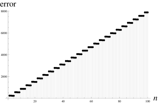
In the framework of the standard Padé scheme, one comes to a strongly divergent sequence, as is seen in Fig. 13.

Figure 13: Error function. Percentage errors for the amplitude, with increasing approximation order, obtained with the standard Padé approximants.

In the framework of the corrected Padé scheme, with the control function

$$K(x)=R_{3}^{*}(x)=\frac{x}{\sqrt[6]{\frac{16x^{6}}{63}+\left(\frac{32x^{4}}{45}+\frac{4x^{2}}{3}+1\right)^{3/2}}}\;,$$ (42)

good numerical convergence is achieved, as is shown in Fig. 14.

Figure 14: Error function. Percentage errors for the amplitude, with increasing approximation order, obtained with corrected approximants.

7.4 Debye function

Let us consider the Debye function

$$D_{1}(x)=\frac{1}{x}\int_{0}^{x}\frac{y}{\exp(y)-1}\,dy\;.$$ (43)

For large $x$,

$$D_{1}(x)\simeq Ax^{-1}\;,$$

with the amplitude at infinity

$$A=\frac{\pi^{2}}{6}\approx 1.64493\;.$$

The expansion for small $x$ reads as

$$D_{1}(x)\approx 1-\frac{x}{4}+\frac{x^{2}}{36}-\frac{x^{4}}{3600}+\frac{x^{6}}{211680}+O(x^{8})\;.$$ (44)

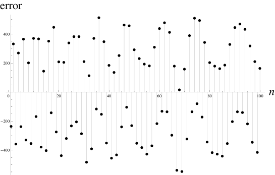
The standard Padé approximations fail completely, following a rather chaotic pattern, as is shown in Fig. 15

Figure 15: Debye function. Percentage errors for the amplitude, with increasing approximation order, obtained with the standard Padé approximants.

The control function, playing the role of the initial approximation, is

$$K(x)=R_{2}^{*}(x)=\frac{1}{\sqrt{\frac{5x^{2}}{72}+\left(\frac{x}{4}+1\right)^{2}}}\;.$$ (45)

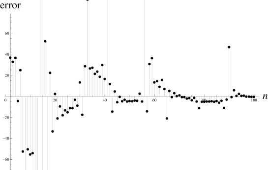
The corresponding corrected Padé approximants work well, providing rather good accuracy, as is shown in Fig. 16.

Figure 16: Debye function. Percentage errors for the amplitude, with increasing approximation order, obtained with the corrected Padé approximants. The number $n$ changes from $n=1$ to $n=100$.

7.5 Connected moments

An example from Ref. [39] concerns the application of the method of connected moments to the calculation of the ground state energy of a harmonic oscillator as the limit of generating function moments, as ”time” $t$ goes to infinity.

The generating function for the harmonic oscillator is

$$E(t)=\frac{121u(t)^{3}+189199u(t)^{2}+8180919u(t)+6561}{(81-u(t))\left(121u(t)^{2}+20198u(t)+81\right)}\;,$$ (46)

where $u(t)=\exp(-4t)$.

The $t$-expansion was also applied earlier to the case of $1d$ -antiferromagnet [40], but there are just a few starting terms in this $t$-expansion.

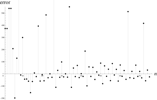
The standard Padé scheme for eq. (46) shows no convergence, as is evident from the corresponding Fig. 17.

Figure 17: Generating function. Percentage errors for the amplitude, with increasing approximation order, obtained with the standard Padé approximants.

Bur the corrected Padé approximants demonstrate rather good convergence, with a simple control function corresponding to the shifted root approximant

$$K(t)=v_{2}+v_{3}(v_{4}t+1)^{-c}\;,$$ (47)

where

$$v_{2}=\frac{403171240048919}{85626857995920},\quad v_{3}=\frac{36337990380139}{85626857995920},\quad v_{4}=\frac{2331886111}{1340069829},\quad c=\frac{9}{10}\;.$$

The results of calculations, corresponding to the corrected Padé scheme, are shown in Fig. 18.

Figure 18: Generating function. Percentage errors for the amplitude, with increasing approximation order, obtained with the corrected Padé approximants.

8 Massive Schwinger model in lattice theory

In the previous sections, we have illustrated the method of corrected Padé approximants for several simple cases. Now we show its applicability for more complicated cases that are of physical interest.

In the present section, we consider the massive Schwinger model in Hamiltonian lattice theory [41, 42]. This model describes quantum electrodynamics in two space-time dimensions. Its fascinating features include many of the properties of quantum chromodynamics, such as confinement, chiral symmetry breaking, and a topological vacuum. Because of these effects, the Schwinger model has attracted great interest.

Let us consider the energy gap between the lowest and first excited states of the vector boson, which can be represented as a function $\Delta(z)$ of the variable

$$z=x^{2}\;,\qquad x\equiv\frac{1}{g^{2}a^{2}}\;,$$ (48)

where $g$ is a coupling parameter and $a$ is lattice spacing. The gap can be expressed as an expansion

$$\Delta(z)\simeq\sum_{n}a_{n}z^{n}\qquad(z\rightarrow 0)$$ (49)

in powers of asymptotically small $z$, when the coupling parameter is strong. The coefficients here are

$$a_{0}=1\;,\qquad a_{1}=2\;,\qquad a_{2}=-10\;,$$

$$a_{3}=78.66667\;,\qquad a_{4}=-736.2222\;,\qquad a_{5}=7572.929\;,$$

$$a_{6}=-82736.69\;,\qquad a_{7}=942803.4\;.$$

The strong increase of the coefficients makes the series in powers of $z$ widely divergent.

However, the transition from the lattice formulation to the continuous limit requires taking the limit $a\rightarrow 0$, which implies $z\rightarrow\infty$. In this limit, the gap behaves as

$$\Delta(z)\simeq 0.5642z^{1/4}\qquad(z\rightarrow\infty)\;.$$ (50)

Using Padé approximants, we get $A_{7}=0.680043$, with the percentage error of $21\%$. While employing the corrected Padé approximants, with the control function

$$K(z)=R_{2}^{*}(z)=\left((1+8z)^{2}-32z^{2}\right)^{1/8}\;,$$

we find $A_{7}=0.591181$, with the error of $4.8\%$, which is essentially better than the standard approach.

9 Critical temperature of weakly interacting Bose gas

Three-dimensional Bose gas, at low temperature experiences Bose-Einstein condensation at a critical temperature $T_{c}$. The properties of Bose-condensed gas have recently been intensively studied both theoretically and experimentally (see recent books and review articles ([43, 44, 45, 46, 47, 48]). An interesting problem is the calculation of the critical temperature $T_{c}$ of weakly interacting uniform Bose gas, as compared to the Bose-condensation temperature of ideal gas

$$T_{0}=\frac{2\pi}{m}\;\left[\frac{\rho}{\zeta(3/2)}\right]^{2/3}\;,$$ (51)

where $m$ is atomic mass and $\rho$, average density. The Planck and Boltzmann constants are set to one.

The difficulty of this problem is that the ideal Bose gas and interacting Bose gas are in different classes of universality, so that the transition from the ideal gas to the interacting one cannot be done by simple perturbation theory [49].

One considers the relative critical temperature shift

$$\frac{\Delta T_{c}}{T_{0}}\equiv\frac{T_{c}-T_{0}}{T_{0}}\;,$$ (52)

which, at weak interaction, can be presented by the expression

$$\frac{\Delta T_{c}}{T_{0}}\simeq c_{1}\gamma\qquad(\gamma\rightarrow 0)\;,$$ (53)

as a function of the gas parameter

$$\gamma\equiv\rho^{1/3}a_{s}\;,$$ (54)

with $a_{s}$ being scattering length.

The coefficient $c_{1}$, for the two-component $O(2)$ field theory, describing the real interacting Bose gas, has been calculated by different ways, including Ursel operator techniques [50] ($c_{1}=1.95$), renormalization-group methods [51, 52, 53] ($c_{1}=1.15-1.37$). Optimized perturbation theory [54, 55] has been used for calculating $c_{1}$ by either introducing control functions into an initial Lagrangian [56, 57, 58, 59, 60, 61] or into a variable transformation [62, 63, 64, 65]. Control functions are defined by optimization conditions, among which the most often used are the variational and finite-difference conditions [66, 67, 68]. These conditions are equivalent to each other and, for defining $c_{1}$, lead to very close results [59]. Optimized perturbation theory, with increasing order, numerically converges [59, 69, 70] to the value of the coefficient $c_{1}$ close to that found in Monte Carlo simulations [71, 72, 73] ($c_{1}=1.32\pm 0.02$) and [74] ($c_{1}=1.29\pm 0.05$). The critical temperature for larger values of the gas parameter has also been studied by Monte Carlo simulations [75]. And the critical temperature of the $O(N_{1})\times O(N_{2})$ field theory has been calculated by optimized perturbation theory [76]. A more detailed account of different attempts of calculating $T_{c}$ can be found in Refs. [77, 78, 79].

This brief discussion illustrates the importance of calculating the critical temperature in the $O(N)$ field theory. Here we show how the critical temperature can be easily found by the method of corrected Padé approximants.

Let us start with the seven-loop expansion [65] for the parameter $c=c(x)$,

$$c_{1}(x)\simeq a_{1}x+a_{2}x^{2}+a_{3}x^{3}+a_{4}x^{4}+a_{5}x^{5}\;,$$ (55)

derived for an asymptotically small variable $x\rightarrow 0$, with

$$a_{1}=0.223286\;,\qquad a_{2}=-0.0661032\;,\qquad a_{3}=0.026446\;,$$

$$a_{4}=-0.0129177\;,\qquad a_{5}=0.007290373\;.$$

But the sought value of $c_{1}$ corresponds to the limit

$$c_{1}=\lim_{x\rightarrow\infty}c_{1}(x)\;.$$ (56)

In the calculations of Kastening [65], the variable transformation $x=z/(1-z)^{1/\omega}$ is used, so that $x\rightarrow\infty$ as $z\rightarrow 1$. The obtained results essentially depend on the chosen value of $\omega$, for different choices varying between $c_{1}=1.161$ and $c_{1}=1.376$. It is also worth mentioning that it would be possible to invoke other variable transformations. However, as is known [80], different variable changes can strongly influence the sought limits.

The best Padé approximant $P_{2/3}$ yields the value $c_{1}=0.982$, which is rather far from the Monte Carlo results. Employing the method of corrected Padé approximants, with the control function

$$K(x)=R_{2}^{*}(x)=\frac{0.223286x}{((1+0.296x)^{2}-0.0616x^{2})^{1/2}}\;,$$

we find $c_{1}=1.386$, which is closer to the Monte Carlo results.

In the same way, it is straightforward to find the values of $c_{1}$ for the $O(1)$ field theory, for which the seven-loop expansion [65] gives form (55) with the coefficients

$$a_{1}=0.334931\;,\qquad a_{2}=-0.178478\;,\qquad a_{3}=0.129786\;,$$

$$a_{4}=-0.115999\;,\qquad a_{5}=0.120433\;.$$

The best Padé approximant gives $c_{1}=0.824$, which is much lower than the Monte Carlo result [81] equal to $c_{1}=1.09\pm 0.09$. Resorting to the corrected Padé approximants, with the control function $R_{2}^{*}(x)$, we find $c_{1}=1.207$, which is a bit higher than the Monte Carlo value.

For the $O(4)$ field theory, the seven-loop expansion yields the coefficients

$$a_{1}=0.167465\;,\qquad a_{2}=-0.0297465\;,\qquad a_{3}=0.00700448\;,$$

$$a_{4}=-0.00198926\;,\qquad a_{5}=0.000647007\;.$$

The best Padé approximant yields $c_{1}=1.219$, which is lower than the Monte Carlo result [81] giving $c_{1}=1.6\pm 0.1$. By using the method of corrected Padé approximants, again with the control function $R_{2}^{*}(x)$, we obtain $c_{1}=1.6$ coinciding with the Monte Carlo result.

10 Equation of state for hard-sphere fluids

The structure of many real fluids is mainly determined by repulsive forces, because of which the hard-sphere fluid is the simplest and the most widely used model for describing the behaviour of real fluids.

The equation of state of hard-sphere fluids is characterized [82] by the so-called compressibility factor

$$Z\equiv\frac{P}{\rho k_{B}T}=Z(y)\qquad\left(y\equiv\frac{\pi\rho}{6}\right)\;,$$ (57)

where $P$ is pressure, $\rho$ is density, $T$ is temperature, and $y\equiv\pi\rho/6$ is packing fraction. This factor is usually represented by the virial expansion

$$Z=1+\sum_{n=2}^{\infty}B_{n}y^{n-1}\;.$$ (58)

The virial coefficients $B_{n}$ do not depend on temperature and are defined in terms of integrals whose integrands are products of Mayer functions. Only the first four virial coefficients can be calculated analytically:

$$B_{1}=1\;,\qquad B_{2}=4\;,\qquad B_{3}=10\;,$$

$$B_{4}=\frac{2707\pi+[438\sqrt{2}-4131\arccos(1/3)]}{70\pi}\;=18.364768\;.$$

The higher virial coefficients have been calculated [83, 84] numerically:

$$B_{5}=28.224512\;,\qquad B_{6}=39.815148\;,\qquad B_{7}=53.344420\;,$$

$$B_{8}=68.537549\;,\qquad B_{9}=85.812838\;,\qquad B_{10}=105.775104\;,$$

$$B_{11}=127.93\;,\qquad B_{12}=152.67\;,\qquad B_{13}=181.19\;,$$

$$B_{14}=214.75\;,\qquad B_{15}=246.96\;,\qquad B_{16}=279.17\;.$$

The values of the virial coefficients increase with the expansion order, because of which this expansion is strongly divergent.

In order to get an equation of state, one either employs Padé approximants complimented by some phenomenological terms or constructs purely phenomenological equations. The standard way of checking the validity of the so constructed equations is as follows. One forms an equation exactly reproducing the first ten virial coefficients. Then this equation is expanded in powers of the packing fraction $y$ and one examines how such an expansion reproduces the last virial coefficients from $B_{11}$ to $B_{16}$. The maximal error in reproducing these last virial coefficients defines the accuracy of the studied equation of state. The analysis of a great number of different equations of states has been accomplished in Refs. [85, 86, 87]. Referring to these papers, we give below a brief account of their findings.

One of the most popular equations is the Cannahan-Starling equation, which has the structure of a $P_{3/3}$ Padé approximant. This equation reproduces the higher virial coefficients with a maximal error of $3.6\%$.

Clisby and McCoy proposed the $P_{4/5}$ and $P_{5/4}$ Padé approximants, whose maximal errors in the reproduction of higher virial coefficients are $9.1\%$ and $7.1\%$, respectively.

Kolafa, Labik, and Malijevsky suggested the equations in the form of series in powers of $y/(1-y)$, with the parameters fitted to the lower densities. Two fitting procedures lead to the reproduction of the higher virial coefficients with the errors $75\%$ and $34\%$.

Liu suggested a phenomenological combination of Padé approximants and power series, with the maximal error of $15\%$.

Santos and Lopez de Haro proposed a phenomenological equation, having the error of $8.9\%$.

Tian, Jiang, Gui, and Mulero [86] constructed a phenomenological equation as a Laurent series in powers of $y-b$. As they write, it was possible to construct $57$ different variants of such equations, the best of which reproduces the higher virial coefficients with an error of $3.2\%$.

Applying the method of corrected Padé approximants, it is convenient, first, to introduce the notation

$$x=\frac{y}{1-y}\qquad\left(y=\frac{x}{1+x}\right)\;,$$ (59)

such that $x\rightarrow\infty$, when $y\rightarrow 1$. This allows us to use the standard techniques of Sec. 2 by considering the limit $x\rightarrow\infty$.

As follows from some phenomenological equations [85, 86, 87], for instance, from the Cannahan-Starling equation, the compressibility factor in the vicinity of $y=1$ behaves as

$$Z(y)\simeq\frac{2}{(1-y)^{3}}\qquad(y\rightarrow 1)\;.$$

Hence, in terms of the variable $x$, we have

$$Z(y(x))\simeq 2x^{3}\qquad(x\rightarrow\infty)\;.$$ (60)

Following the scheme of Sec. 2, we take as a control function the second-order root approximant

$$K(x)=R_{2}^{*}(x)=\left(\left(1+\frac{4}{3}\;x\right)^{2}+\frac{4}{9}\;x^{2}\right)^{3/2}\;.$$ (61)

For the ratio $Z(y)/K(x(y))$, we construct a corrected Padé approximant $P_{5/5}(y)$ taking into account the first ten virial coefficients. Then the resulting equation of state is

$$Z^{*}(y)=K(x(y))P_{5/5}(y)\;.$$ (62)

This equation predicts the higher virial coefficients, up to $B_{16}$, with an error not exceeding $2.5\%$.

Note that the method of estimating the accuracy of the approach by predicting the higher-order coefficients goes back to Feynman, as discussed in Ref. [88].

11 Fluctuating pressure of fluid membrane

Membranes are frequent structures in various biological, chemical, and mechanical systems, whose description is not easy. One of the often met types is a fluid membrane between two fixed boundaries. To calculate the pressure of this membrane, one introduces a potential of strength $\lambda$ between two walls at distance $L$. Then the membrane pressure, in dimensionless units, can be represented as a function $p(x)$ of a variable $x=1/(\lambda L)^{2}$, yielding [36] the expansion

$$p(x)\simeq\frac{\pi^{2}}{8x^{2}}\sum_{n=0}^{k}a_{n}x^{n}\;,$$ (63)

when $x\rightarrow 0$, with the coefficients

$$a_{0}=1\;,\qquad a_{1}=\frac{1}{4}\;,\qquad a_{2}=\frac{1}{32}\;,\qquad a_{3}=2.176347\times 10^{-3}\;,$$

$$a_{4}=0.552721\times 10^{-4}\;,\qquad a_{5}=-0.721482\times 10^{-5}\;,\qquad a_{6}=-1.777848\times 10^{-6}\;.$$

But in order to return to the case of a membrane between two rigid walls, one has to remove the auxiliary potential, setting $\lambda\rightarrow 0$, when $x\rightarrow\infty$. Hence, one needs to find the limit

$$p=\lim_{x\rightarrow\infty}p(x)\;.$$

Several attempts employing directly Padé approximants, as well as other approximants [89], have been shown to give bad accuracy, with the best Padé approximants giving $p=0.015$, which is quite far form the value

$$p=0.0798\pm 0.0003$$

obtained in Monte Carlo simulations [90]. A closer to the Monte Carlo result was found by Kastening [36] by employing optimized perturbation theory, with introducing control functions through a change of variables [77]. As has been mentioned above, the results essentially depend on the kind of the variable transformation. Kastening found $p=0.0821$, which is $3\%$ higher than the Monte Carlo value. Below, we show how an accurate value for the limit $p(\infty)$ can be easily derived by means of corrected Padé approximants.

Following the method of corrected Padé approximants, with the control function in the form of a root approximant

$$K(x)=\left(\left(\left(1+\frac{1}{8}\;x\right)^{2}+\frac{1}{64}\;x^{2}\right)^{3/2}+A_{3}x^{3}\right)^{2/3}\;,$$ (64)

where $A_{3}=0.00326452$, we consider the series for the ratio $p(x)/K(x)$ and construct the Padé approximant $P_{4/4}$, so that the pressure becomes

$$p(x)=\frac{\pi^{2}}{8x^{2}}\;K(x)P_{4/4}(x)\;.$$ (65)

Taking here the limit $x\rightarrow\infty$, we obtain

$$p(\infty)=0.0806\;,$$

which is very close to the Monte Carlo value, deviating from it only by $1\%$.

12 Conclusion

We have suggested a method of corrected Padé approximants, whose idea is based on using as an initial approximation a self-similar approximant taking into account irrational features of the sought function. We showed that the suggested method covers a much broader class of functions than the standard Padé approximants do, including the cases of indeterminate problems. The corrected Padé approximants are easy to construct. Their computational accuracy, when the standard Padé scheme appears to converge, is either close to that of diagonal Padé approximants, when these exist, or is essentially better, making the rate of convergence faster.

But most importantly, the corrected scheme works well, even when the standard Padé scheme completely fails, being either divergent or not defined at all.

We have illustrated the advantage of the suggested corrected Padé approximants by several simple functions related to physical applications. Also, we demonstrated the efficiency of the method for several complicated physical problems, such as the massive Schwinger model in lattice field theory, the scalar field theory $O(N)$ having to do with the phase transition in Bose gases, the equation of state for hard-sphere fluids, and fluctuating pressure of a fluid membrane. The method of corrected Padé approximants is shown to combine rather easy calculations with good accuracy.

References

- [1] G.A. Baker, P. Graves-Moris, Padé Approximants (Cambridge University, Cambridge, 1996).
- [2] S.P. Suetin, Padé approximants and efficient analytic continuation of power series, Rus. Math. Surv. 57, 43–141 (2002).
- [3] A.A. Gonchar, Rational approximation of analytic functions, Proc. Steklov Math. Inst. 272 (Suppl. 2), 44–57 (2011).
- [4] G.A. Baker, J.L. Gammel, The Padé approximant, J. Math. Anal. Appl. 2, 21–30 (1961).
- [5] C.M. Bender, S. Boettcher, Determination of from the asymptotoc series for about , J. Math. Phys. 35, 1914–1921 (1994).
- [6] D.S. Lubinsky, Reflections on the Baker-Gammel-Wills (Padé ) conjecture, in: Analytic Number Theory, Approximation Theory, and Special Functions, p. 561–571 (Springer, New York, 2014).
- [7] M.G. Krein, A.A. Nudel’man, The Markov Moment Problem and Extremal Problems (American Mathematical Society, Providence, 1977).
- [8] H.S. Wall, Analytic Theory of Continued Fractions (Chelsea Publishing Company, New York, 1948).
- [9] W. Van Assche, The impact of Stieltjes work on continued fractions and orthogonal polynomials, in: Thomas Jan Stieltjes Oeuvres Complètes - Collected Papers, G. van Dijk, ed., pp. 5–37 (Springer, Berlin, 1993).
- [10] G. Valent, W. Van Assche, The impact of Stieltjes’ work on continued fractions and orthogonal polynomials: additional material, J. Comput. Appl. Math. 65, 419–447 (1995).
- [11] V.M. Adamyan, O.I. Gerasimov, Statistical structure of the energy loss spectrum of charged particles scattered in disordered media, Theor. Math. Phys. 74, 279–287 (1988).
- [12] V.M. Adamyan, I.M. Tkachenko, M. Urrea, Solution of the Stieltjes truncated moment problem, J. Appl. Anal. 9, 57–74 ( 2003).
- [13] N.P. Malomuzh, M.Y. Sushko, On the character of narrowing of spectral lines near the phase transition isotropic liquid-nematic, Opt. Spectrosc. 62, 386–391 (1987).
- [14] C. Berg, Indeterminate moment problems and the theory of entire functions, J. Comput. Appl. Math. 65, 27–55 (1995).
- [15] W. Van Assche, Padé and Hermite-Padé approximation and orthogonality, Surveys Approx. Theory 2, 61–91 (2006).
- [16] A.V. Sergeev, D.Z. Goodson, Summation of asymptotic expansions of multiple-valued functions using algebraic approximants: Application to anharmonic oscillators. J. Phys. A 31, 4301–4317 (1998).
- [17] V.I. Yukalov, Method of self-similar approximations, J. Math. Phys. 32, 1235–1239 (1991).
- [18] V.I. Yukalov, Stability conditions for method of self-similar approximations, J. Math. Phys. 33, 3994–4001 (1992).
- [19] S. Gluzman, V.I. Yukalov, Self-similar extrapolation from weak to strong coupling, J. Math. Chem. 48, 883–913 (2010).
- [20] S. Gluzman, V.I. Yukalov, Extrapolation of perturbation-theory expansions by self-similar approximants, Eur. J. Appl. Math. 25, 595–628 (2014).
- [21] S. Gluzman, V.I. Yukalov, D. Sornette, Self-similar factor approximants, Phys. Rev. E 67, 026109 (2003).
- [22] V.I. Yukalov, S. Gluzman, D. Sornette, Summation of power series by self-similar factor approximants, Physica A, 328, 409–438 (2003).
- [23] V.I. Yukalov, E.P. Yukalova, S. Gluzman, Self-similar interpolation in quantum mechanics, Phys. Rev. A 58, 96–115 (1998).
- [24] F.M. Fernandez, Introduction to Perturbation Theory in Quantum Mechanics (CRC, Boca Raton, 2000).
- [25] S. Gluzman, V.I. Yukalov, Unified approach to crossover phenomena, Phys. Rev. E 58, 4197–4209 (1998).
- [26] S. Gluzman, V.I. Yukalov, Self-similar continued root approximants, Phys. Lett. A 377, 124–128 (2012).
- [27] V.I. Yukalov, S. Gluzman, Self-similar interpolation in high-energy physics, Phys. Rev. D 91, 125023 (2015).
- [28] A. Ambroladze, H. Wallin, Approximation by repeated Padé approximants, J. Comput. Appl. Math. 62, 353–358 (1995).
- [29] A. Ambroladze, H. Wallin, Convergence rates of Padé and Padé -type approximants, J. Approx. Theor. 86, 310–319 (1996).
- [30] F. Mainardi, R. Goren, On Mittag-Leffler-type functions in fractional evolution processes, J. Comput. Appl. Math. 118, 283–299 (2000).
- [31] C. Bender, T. Wu, Anharmonic oscillator, Phys. Rev. 184, 1231–1260 (1969).
- [32] T. Karasudani, T.K. Nagano, H. Okamoto, H. Mori, A new continued-fraction representation, Prog. Theor. Phys. 61, 850–863 (1979).
- [33] A.Y. Grosberg, A.R. Khokhlov, Statistical Physics of Macromolecules (American Insitute of Physics, New York, 1994).
- [34] P.M. Lam, The structure function of branched polymers in a good solvent: a lattice calculation, J. Chem. Phys. 92, 3136–3143 (1990).
- [35] J.D. Miller, J Exact pair correlation function of a randomly branched polymer, Eur. Phys. Lett. 16, 623–628 (1991).
- [36] B. Kastening, Fluctuation pressure of a fluid membrane between walls through six loops, Phys. Rev. E 73, 011101 (2006).
- [37] H.S. Wilf, Generating Functionology (Academic Press, Boston, 1994).
- [38] T. Banks, T.J. Torres, Two point Padé approximants and duality, arXiv:1307.3689 (2013).
- [39] F.M. Fernandez, Prony’s method and the connected-moments expansion, Phys. Scr. 87, 025006 (2013).
- [40] D. Horn, M. Weinstein, The -expansion: a nonperturbative analytic tool for Hamiltonian systems, Phys. Rev. D 30, 1256–1270 (1984).
- [41] J. Schwinger, Gauge invariance and mass, Phys. Rev. 128, 2425–2428 (1962).
- [42] C.J. Hamer, Z. Weihong, J. Oitmaa, Series expansions for the massive Schwinger model in Hamiltonian lattice theory, Phys. Rev. D 56, 55–67 (1997).
- [43] C.J. Pethick, H. Smith, Bose Einstein Condensation in Dilute Gases (Cambridge University, Cambridge, 2002).
- [44] E.H. Lieb, R. Seiringer, J.P. Solovej, J. Yngvason, The Mathematics of the Bose Gas and its Condensation (Birkhauser, Basel, 2005).
- [45] V. Letokhov, Laser Control of Atoms and Molecules (Oxford University, New York, 2007).
- [46] . V.I Yukalov, Cold bosons in optical lattices, Laser Phys. 19, 1–110 (2009).
- [47] V.I. Yukalov, Basics of Bose-Einstein condensation, Phys. Part. Nucl. 42, 460–513 (2011).
- [48] V.I. Yukalov, Theory of cold atoms: Bose-Einstein statistics, Laser Phys. 26, 062001 (2016).
- [49] M. Holzmann, J.N. Fuchs, G. Baym, J.P. Blaizot, F. Laloë, Bose-Einstein condensation temperature in a dilute repulsive gas, Compt. Rend. Phys. 5, 21–37 (2004).
- [50] G. Baym, J.P. Blaizot, M. Holzmann, F. Laloë, D. Vautherin, Bose-Einstein transition in a dilute interacting gas, Eur. Phys. J. B 24, 107–124 (2001).
- [51] S. Ledowski, N. Hasselmann, P. Kopietz, Self-energy and critical temperature of weakly interacting bosons, Phys. Rev. A 69, 061601 (2004).
- [52] J.P. Blaizot, R. Mendez-Galain, N. Wschebor, Non-perturbative renormalization group calculations of the transition temperature of the weakly interacting Bose gas, Eur. Phys. Lett. 72, 705–711 (2005).
- [53] F. Benitez, J.P. Blaizot, H. Chate, B. Delamotte, R. Mendez-Galain, N. Wschebor, Phys. Rev. E 80, 030103 (2009).
- [54] V.I. Yukalov, Theory of perturbations with a strong interaction, Moscow Univ. Phys. Bull. 31, 10–15 (1976).
- [55] V.I. Yukalov, Model of a hybrid crystal, Theor. Math. Phys. 28, 652–660 (1976).
- [56] F.F. de Souza Cruz, M.B. Pinto, R.O. Ramos, Critical temperature shift in dilute Bose gas, Laser Phys. 12, 203–206 (2002).
- [57] F.F. de Souza Cruz, M.B. Pinto, R.O. Ramos, Transition temperature for weakly interacting homogeneous Bose gases, Phys. Rev. B 64, 014515 (2001).
- [58] F.F. de Souza Cruz, M.B. Pinto, R.O. Ramos, P. Senna, Higher-order calculation of the critical temperature for interacting homogeneous dilute Bose gases, Phys. Rev. A 65, 053613 (2002).
- [59] J.L. Kneur, M.B. Pinto, R.O. Ramos, Convergent resummed linear delta expansion in the critical model, Phys. Rev. Lett. 89, 210403 (2002).
- [60] J.L. Kneur, M.B. Pinto, R.O. Ramos, Asymptotically improved convergence of optimized perturbation theory in the Bose-Einstein condensation problem, Phys. Rev. A 68, 043615 (2003).
- [61] J.L. Kneur, A. Neveu, M.B. Pinto, Improved optimization of perturbation theory: applications to the oscillator energy levels and Bose-Einstein condensate critical temperature, Phys. Rev. A 69, 053624 (2004).
- [62] H. Kleinert, Five-loop critical temperature shift in weakly interacting homogeneous Bose-Einstein condensate, Mod. Phys. Lett. B 17, 1011–1020 (2003).
- [63] B. Kastening, Bose-Einstein condensation temperature of a homogeneous weakly interacting Bose gas in variational perturbation theory through six loops, Phys. Rev. A 68, 061601 (2003).
- [64] B. Kastening, Shift of BEC temperature of homogeneous weakly interacting Bose gas, Laser Phys. 14, 586–590 (2004).
- [65] B. Kastening, Bose-Einstein condensation temperature of a homogeneous weakly interacting Bose gas in variational perturbation theory through seven loops, Phys. Rev. A 69, 043613 (2004).
- [66] E.P. Yukalova, V.I. Yukalov, Self-similar approximation for an anharmonic oscillator of arbitrary dimensionality, Phys. Lett. A 175, 27–35 (1993).
- [67] E.P. Yukalova, V.I. Yukalov, Self-similar eigenvalues for Schrödinger operators with power-law potentials, Phys. Scr. 47, 610–617 (1993).
- [68] V.I. Yukalov, E.P. Yukalova, Self-similar structures and fractal transforms in approximation theory, Chaos Solit. Fract. 14, 839–861 (2002).
- [69] E. Braaten, E. Radescu, Covergence of the linear delta expansion in the critical field theory, Phys. Rev. Lett. 89, 271602 (2002).
- [70] E. Braaten, E. Radescu, Convergence of the linear delta expansion for the shift in for Bose-Einstein condensation, Phys. Rev. A 66, 063601 (2002).
- [71] P. Arnold, G. Moore, BEC transition temperature of a dilute homogeneous imperfect Bose gas, Phys. Rev. Lett. 87, 120401 (2001).
- [72] P. Arnold, G. Moore, Monte Carlo simulation of field theory in three dimensions, Phys. Rev. E 64, 066113 (2001).
- [73] P. Arnold, G. Moore, B. Tomasik, for homogeneous dilute Bose gases: a second-order result, Phys. Rev. A 65, 013606 (2001).
- [74] V.A. Kashurnikov, N. Prokofev, B. Svistunov, Critical temperature shift in weakly interacting Bose gas, Phys. Rev. Lett. 87, 120402 (2001).
- [75] S. Pilati, S. Giorgini, N. Prokofev, Critical temperature of interacting Bose gases in two and three dimensions, Phys. Rev. Lett. 100, 140405 (2008).
- [76] M.B. Pinto, R.O. Ramos, Nonperturbative study of inverse symmetry breaking at high temperatures, Phys. Rev. D 61, 125016 (2000).
- [77] H. Kleinert, Path Integrals (World Scientific, Singapore, 2003).
- [78] J.O. Andersen, Theory of the weakly interacting Bose gas, Rev. Mod. Phys. 76, 599–639 (2004).
- [79] V.I. Yukalov, Principal problems in Bose-Einstein condensation of dilute gases, Laser Phys. Lett. 1, 435–461 (2004).
- [80] D.H. Bailey, J.M. Borwein, D. Broadhurst, W. Zudlin, Experimental mathematics and mathematical physics, Contemp. Math. 517, 41–58 (2010).
- [81] X. Sun, Monte Carlo studies of three-dimensional and theory related to Bose-Einstein condensation phase transition temperatures Phys. Rev. E 67, 066702 (2003).
- [82] A. Mulero, Theory and Simulation of Hard-Sphere Fluids and Related Systems (Springer, Berlin, 2008).
- [83] N. Clisby, B.M. McCoy, New results for virial coefficients of hard spheres in dimensions, Pramana J. Phys. 64, 775–783 (2005).
- [84] N. Clisby, B.M. McCoy, Ninth and tenth order virial coefficients for hard spheres in dimensions, J. Stat. Phys. 122, 15–57 (2006).
- [85] G.W. Wu, R.J. Sadus, Hard sphere compressibility factors for equation of state development, Am. Inst. Chem. Eng. J. 51, 309–313 (2005).
- [86] J. Tian, H. Jiang, Y. Gui, A. Mulero, Equation of state for hard-sphere fluids offering accurate virial coefficients, Phys. Chem. Chem. Phys. 11, 11213–11218 (2009).
- [87] J. Tian, Y. Gui, A. Mulero, New closed equation of state for hard-sphere fluids, J. Phys. Chem. B 114, 13399–13402 (2010).
- [88] M.A. Samuel, G. Li, Estimating perturbative coefficients in quantum field theory and the ortho-positronium decay rate discrepancy, Phys. Lett. B 331, 114–118 (1994).
- [89] V.I. Yukalov, S. Gluzman, Extrapolation of power series by self-similar factor and root approximants, Int. J. Mod. Phys. B 18, 3027–3046 (2004).
- [90] G. Gompper, D. M. Kroll, Steric interactions in multimembrane systems: a Monte Carlo study, Eur. Phys. Lett. 9, 59–64 (1989).