Cross-correlation of CFHTLenS galaxy catalogue and Planck CMB lensing using the halo model prescription

Abstract

Aims. I cross-correlate the galaxy counts from the Canada-France Hawaii Telescope Lensing Survey (CFHTLenS) galaxy catalogue and cosmic microwave background (CMB) convergence from the Planck data releases 1 (2013) and 2 (2015).

Methods. I improve on an earlier study by computing an analytic covariance from the halo model, implementing simulations to validate the theoretically estimated error bars and the reconstruction method, fitting both a galaxy bias and a cross-correlation amplitude using the joint cross and galaxy auto-correlation, and performing a series of null tests.

Results. Using a Bayesian analysis, I find a galaxy bias $b=0.92_{-0.02}^{+0.02}$ and a cross-correlation amplitude $A=0.85_{-0.16}^{+0.15}$ for the 2015 release, whereas for the 2013 release, I find $b=0.93_{-0.02}^{+0.02}$ and $A=1.05_{-0.15}^{+0.15}$.

Conclusions. I thus confirm the difference between the two releases found earlier, although both values of the amplitude now appear to be compatible with the fiducial value $A=1$.

1 Introduction

In the framework of the standard cosmological model, galaxies form in matter overdensities that are the result of the non-linear growth of primordial inhomogeneities generated by inflation. As a photon travels from its surface of last scattering to us, its path is deflected by the large-scale structures of the universe. Studying this weak gravitational lensing of the cosmic microwave background (CMB), which is characterized by temperature and polarization anisotropies, allows us to reconstruct a map of the integrated (over the line of sight) overdensity of matter of the universe (Okamoto & Hu, 2003).

Galaxies are expected to form inside dark matter halos, situated at the peaks of the density fluctuations. Galaxies are therefore expected to be good tracers of the large-scale structures, although their clustering characteristics may be different from the dark matter ones. The ratio between galaxy counts fluctuations and dark matter fluctuations is called the galaxy bias. Studying the cross-correlation of lensing convergence with galaxies allows this galaxy bias to be determined by a method possibly free of unaccounted-for correlated systematics effects, contrary to the auto-correlation of galaxies.

Several galaxy catalogues have been cross-correlated with the lensing convergence: Planck CMB lensing cross-correlated with NVSS quasars, MaxBCG clusters, SDSS LRGs, and the WISE Catalogue (Planck Collaboration et al., 2014), with the CFHTLenS galaxy catalogue (Omori & Holder, 2015) and with high-z submillimetre galaxies detected by the Herschel-ATLAS survey (Bianchini et al., 2015); WMAP lensing cross-correlated with NVSS galaxies (Smith et al., 2007) and with LRGs and quasars from SDSS (Hirata et al., 2008); South Pole Telescope lensing cross-correlated with Blanco Cosmology Survey galaxies (Bleem et al., 2012) and with WISE quasars (Geach et al., 2013); Atacama Cosmology Telescope lensing cross-correlated with SDSS quasars (Sherwin et al., 2012).

In this paper, I cross-correlate the galaxy counts from the Canada-France Hawaii Telescope Lensing Survey (CFHTLenS) (Heymans et al. (2012); Erben et al. (2013)) and the convergence all-sky map from the Planck collaboration (Planck Collaboration et al., 2014; Collaboration et al., 2015) for the 2013 and 2015 releases. I followed the study of Omori & Holder (2015), who found the surprising result of a significant difference between the galaxy bias inferred from the two releases. To complete their work, I computed the theoretical covariances inferred from the halo model (Cooray & Sheth, 2002), fitted the joint cross and auto-correlation, implemented Gaussian simulations to check the error bars and the reconstruction method, and performed a series of null tests. The difference between the two releases, as found by Omori & Holder (2015), is recovered, although it is less significant.

This paper is organized as follows. In Section 2, I present the theoretical background needed for this study and correct some incomplete formulaes from the halo model. Data maps are presented in Section 3, and the joint cross and auto-correlation analysis is performed in Section 4. Section 5 presents the consistency checks I carried out: Gaussian simulations and null tests. Finally in Section 6 I summarize my results.

Throughout this paper, I assume a flat $\Lambda$CDM cosmology with $h=0.70$, $H_{0}=100h\>\mathrm{km\,s^{-1}\,Mpc^{-1}}$, $\Omega_{\Lambda}^{0}=0.7$, $\Omega_{m}^{0}=0.3$, $n_{s}=0.97$, $\sigma_{8}=0.82$, and $a_{0}=1$.

2 Theoretical background

2.1 Cross- and auto-correlation

The effect of weak gravitational lensing by large-scale structures on the CMB photons is described by a distortion matrix $\mathcal{\boldsymbol{\mathcal{A}}}$ that relates the direction of observation $\boldsymbol{\theta}=\left(\theta_{1},\theta_{2}\right)$ and the direction of the unlensed source $\boldsymbol{\theta_{s}}$: $\mathbf{\boldsymbol{\theta}_{s}=\boldsymbol{\mathcal{A}\cdot\theta}}$ with $\mathcal{A}_{ab}=\delta_{ab}-\partial_{\theta_{a}\theta_{b}}\psi\left(\boldsymbol{\theta}\right)$. Here, $\psi$ is the lensing potential given by e.g. Peter & Uzan (2013), pp 398-399:

$$\psi\left(\boldsymbol{\theta}\right)=\frac{2}{c^{2}}\int_{0}^{\chi_{CMB}}\frac{\chi_{CMB}-\chi}{\chi\chi_{CMB}}\Phi\left[\chi\boldsymbol{\theta},\chi\right]d\chi.$$ (1)

In this equation $\chi$ is the line-of-sight comoving distance, $\chi_{CMB}$ is the comoving distance of the CMB at redshift $z_{CMB}\simeq 1090$, and $\Phi$ is the gravitational potential at the point on the photon path given by $\chi\boldsymbol{\theta}$. The lensing convergence $\kappa$ is defined as $\kappa\left(\boldsymbol{\theta}\right)\equiv\triangle_{2}\psi\left(\boldsymbol{\theta}\right)/2$ and is related to the matter overdensity $\delta$ via

$$\kappa\left(\boldsymbol{\theta}\right)=\intop_{0}^{\chi_{CMB}}W^{\kappa}\left(\chi\right)\delta\left(\chi\boldsymbol{\theta},\chi\right)d\chi,$$ (2)

$$W^{\kappa}\left(\chi\right)=\frac{3}{2}\Omega_{m}^{0}\left(\frac{H_{0}}{c}\right)^{2}\frac{\chi\left(\chi_{CMB}-\chi\right)}{\chi_{CMB}}\left(1+z\left(\chi\right)\right).$$ (3)

The overdensity of galaxies is defined as

$$g\left(\boldsymbol{\theta}\right)=\intop_{0}^{\chi_{CMB}}W^{g}\left(\chi\right)\delta\left(\chi\boldsymbol{\theta},\chi\right)d\chi,$$ (4)

$$W^{g}\left(\chi\right)=\frac{dN\left(z\right)}{dz}\frac{dz}{d\chi}b\left(\chi\right)+\frac{3}{2}\Omega_{m}^{0}\left(\frac{H_{0}}{c}\right)^{2}\left(1+z\left(\chi\right)\right)\left(5s-2\right)f\left(\chi\right)$$ (5)

with

$$f\left(\chi\right)=\chi\intop_{\chi}^{\chi_{CMB}}d\chi^{\prime}\frac{\chi^{\prime}-\chi}{\chi^{\prime}}\frac{dN}{dz}\frac{dz}{d\chi^{\prime}}$$ (6)

and

$$s=\frac{d\log_{10}N\left(<m\right)}{dm}.$$

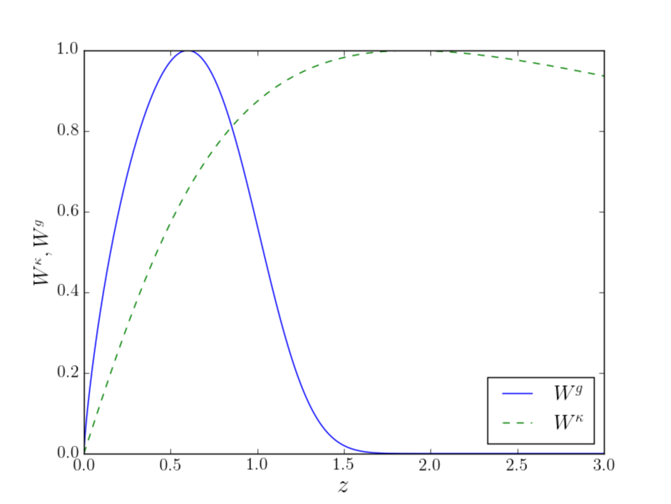
The second term in Equation (5) is the magnification bias (Moessner et al., 1998), which occurs because the number density of galaxies is altered by gravitational lensing; it has an effect of a few percent. The $dN/dz$ ratio is the redshift distribution of the galaxy sample normalized such that $\intop dz\left(dN/dz\right)=1$. The over-density of galaxies is assumed to be linearly proportional to the matter over-density: $\delta^{g}\left(\chi\boldsymbol{\theta},\chi\right)=b\left(\chi\right)\delta\left(\chi\boldsymbol{\theta},\chi\right)$. In this article, the linear bias is assumed to be independent of $\chi$, which is a rather good approximation given the sharply peaked redshift distribution (see Figure 3). The fiducial value adopted for the galaxy bias is $b=1,$ as is suggested in the study of Omori & Holder (2015). Because the effect of the magnification bias is very weak, I take $b$ as an overall factor of $W^{g}$ for simplicity in the fitting algorithm. Figure 1 shows a plot of the two kernels $W^{\kappa}$ and $W^{g}$.

Figure 1: Lensing kernel $W^{\kappa}$ (dashed line) and galaxy overdensity kernel $W^{g}$ (solid line) for all patches of the CFHTLenS catalogue. Both kernels are multiplied by $d\chi/dz$ and normalized to a unit maximum.

Decomposing $\kappa\left(\boldsymbol{\theta}\right)\equiv\sum_{lm}\kappa_{lm}Y_{l}^{m}\left(\boldsymbol{\theta}\right)$ and $g\left(\boldsymbol{\theta}\right)\equiv\sum_{lm}g_{lm}Y_{l}^{m}\left(\boldsymbol{\theta}\right)$ into spherical harmonics and using the Limber approximation (LoVerde & Afshordi, 2008) for small angles, which consists in approximating the spherical Bessel functions by $j_{l}\left(x\right)=\sqrt{\pi/\left(2l+1\right)}\delta_{Dirac}\left(x-l-1/2\right)$ yields

$$C_{l}^{\kappa g}=\intop d\chi\frac{W^{\kappa}\left(\chi\right)W^{g}\left(\chi\right)}{\chi^{2}}P\left(k=\frac{l}{\chi},\,z\left(\chi\right)\right),$$ (7)

where $C_{l}^{\kappa g}$, the cross-correlation between $\kappa$ and $g$, is defined as $\left\langle\kappa_{lm}g_{l^{\prime}m^{\prime}}^{*}\right\rangle=\delta_{ll^{\prime}}\delta_{mm^{\prime}}C_{l}^{\kappa g}$, and $P\left(k,\,z\right)$ is the matter power spectrum, which I compute using the halo model (see Section 2.3) under the convention that

$$\delta\left(\chi\boldsymbol{\theta},\chi\right) \equiv \intop\frac{d^{3}\boldsymbol{k}}{\left(2\pi\right)^{3}}e^{-i\boldsymbol{k}\cdot\left(\chi\boldsymbol{\theta},\chi\right)}\delta\left(\boldsymbol{k}\right)$$ (8)

$$\left\langle\delta\left(\boldsymbol{k}\right)\delta\left(\boldsymbol{k^{\prime}}\right)\right\rangle \equiv \left(2\pi\right)^{3}\delta_{D}\left(\boldsymbol{k}+\boldsymbol{k^{\prime}}\right)P\left(k\right)$$ (9)

$$\left\langle\delta\left(\boldsymbol{k_{1}}\right)\delta\left(\boldsymbol{k_{2}}\right)\delta\left(\boldsymbol{k_{3}}\right)\right\rangle \equiv \left(2\pi\right)^{3}\delta_{D}\left(\boldsymbol{k_{1}}+\boldsymbol{k_{2}}+\boldsymbol{k_{3}}\right)B\left(\boldsymbol{k_{1}},\,\boldsymbol{k_{2}},\,\boldsymbol{k_{3}}\right)$$ (10)

$$\left\langle\delta\left(\boldsymbol{k_{1}}\right)\delta\left(\boldsymbol{k_{2}}\right)\delta\left(\boldsymbol{k_{3}}\right)\delta\left(\boldsymbol{k_{4}}\right)\right\rangle \equiv \left(2\pi\right)^{3}\delta_{D}\left(\boldsymbol{k_{1}}+\boldsymbol{k_{2}}+\boldsymbol{k_{3}}+\boldsymbol{k_{4}}\right)T\left(\boldsymbol{k_{1}},\,\boldsymbol{k_{2}},\,\boldsymbol{k_{3}},\,\boldsymbol{k_{4}}\right)$$

$$...$$

where $\delta_{D}$ stands for the Dirac delta function.

The auto-spectra are computed the same way:

$$C_{l}^{\kappa\kappa}=\intop d\chi\frac{W^{\kappa}\left(\chi\right)^{2}}{\chi^{2}}P\left(k=\frac{l}{\chi},\,z\left(\chi\right)\right)$$ (12)

$$C_{l}^{gg}=\intop d\chi\frac{W^{g}\left(\chi\right)^{2}}{\chi^{2}}P\left(k=\frac{l}{\chi},\,z\left(\chi\right)\right).$$ (13)

I then need an estimator for the cross- and auto-spectra and its covariance, and this is the subject of the next section.

2.2 Estimator

The estimator used for the cross-correlation of the datasets is

$$\tilde{C}_{l_{i}}^{\kappa g}=\frac{1}{f_{sky}}\frac{1}{\left|B_{i}\right|}\sum_{l\in B_{i}}\frac{1}{2l+1}\sum_{m=-l}^{l}\tilde{\kappa}_{lm}\tilde{g}_{lm}^{*},$$ (14)

replacing $g$ with $\kappa$ for the autocorrelations. Quantities with a tilde are observed data, $f_{sky}$ is the fraction of sky covered by the datasets, $B_{i}$ is the bin in $l$ used for the estimator, which is taken in this study as ranging from $l_{min}=50$ to $l_{max}=1950$ with width $\delta l=100$, which corresponds to a number of bins $N_{bin}=19$. The lower $l$ cut is here because of the limited coverage of the sky imposed by the galaxy catalogue, the correlation being meaningful only below a few degrees. I numerically compute the covariance of this estimator using the halo model. Without any other approximation, the full covariance would be too heavy to compute, since it would involve six integrations. That is why I use the flat-sky approximation (Bernardeau et al., 2010), which consists in approximating the sphere by its tangential plane, and so is only valid at small angles. The spherical harmonics transform is then replaced by a simple Fourier transform:

$$\kappa\left(\boldsymbol{l}\right)\equiv\frac{1}{\sqrt{4\pi}}\intop d^{2}\boldsymbol{\theta}e^{i\boldsymbol{l}\cdot\boldsymbol{\theta}}\kappa\left(\boldsymbol{\theta}\right).$$ (15)

The normalization is here to ensure that $\kappa\left(\boldsymbol{0}\right)=\kappa_{00}$. The same equation applies for $g$. Using Equation (2), one finds

$$\kappa\left(\boldsymbol{l}\right)=\frac{1}{\sqrt{4\pi}}\intop_{0}^{\chi_{CMB}}d\chi\frac{W^{\kappa}\left(\chi\right)}{\chi^{2}}\intop_{-\infty}^{+\infty}\frac{dk}{2\pi}\delta\left(\frac{\boldsymbol{l}}{\chi},\,k\right)e^{-ik\chi},$$ (16)

and the correlator is

$$\left\langle\kappa\left(\boldsymbol{l}\right)g^{*}\left(\boldsymbol{l^{\prime}}\right)\right\rangle=\frac{1}{4\pi}\intop d\chi d\chi^{\prime}\frac{W^{\kappa}\left(\chi\right)}{\chi^{2}}\frac{W^{g}\left(\chi^{\prime}\right)}{\chi^{\prime 2}}\left(2\pi\right)^{2}\delta_{D}\left(\frac{\boldsymbol{l}}{\chi}+\frac{\boldsymbol{l^{\prime}}}{\chi^{\prime}}\right)\intop_{-\infty}^{+\infty}\frac{dk}{2\pi}e^{-ik\left(\chi-\chi^{\prime}\right)}P\left(\sqrt{\frac{l^{2}}{\chi^{2}}+k^{2}}\right).$$ (17)

In the small angle approximation, $k$ is neglected before $l/\chi$. (For high values of $k$ the integral is suppressed because of the oscillatory function.) This yields

$$\left\langle\kappa\left(\boldsymbol{l}\right)g\left(\boldsymbol{l^{\prime}}\right)\right\rangle=\pi\delta_{D}\left(\boldsymbol{l}+\boldsymbol{l^{\prime}}\right)C_{l}^{\kappa g}.$$ (18)

The estimator of $C_{l}^{\kappa g}$ in the flat-sky approximation is

$$\tilde{C}_{l_{i}}^{\kappa g}\equiv\frac{1}{f_{sky}}\intop_{\left|l\right|\in B_{i}}\frac{d^{2}\boldsymbol{l}}{\Omega_{i}}\tilde{\kappa}_{\mathcal{W}}\left(\boldsymbol{l}\right)\tilde{g}_{\mathcal{W}}\left(-\boldsymbol{l}\right).$$ (19)

The subscript $\mathcal{W}$ refers to the mask function: Because the different surveys only probe a part of the sky, what is measured is $\tilde{\kappa}_{\mathcal{W}}\left(\boldsymbol{\theta}\right)\equiv\mathcal{W}_{\kappa}\left(\boldsymbol{\theta}\right)\tilde{\kappa}\left(\boldsymbol{\theta}\right)$ and $\tilde{g}_{\mathcal{W}}\left(\boldsymbol{\theta}\right)\equiv\mathcal{W}_{g}\left(\boldsymbol{\theta}\right)\tilde{g}\left(\boldsymbol{\theta}\right)$ with $\mathcal{W}=1$ where the data are not masked and $\mathcal{W}=0$ where the data are masked. Here, $\Omega_{i}\equiv\pi\left(\left(l_{i}+\delta l_{i}\right)^{2}-l_{i}^{2}\right)\simeq 2\pi l_{i}\delta l_{i}$ is the size of the bin $i$, and $f_{sky}\equiv\intop d^{2}\boldsymbol{\theta}\mathcal{W}_{\kappa}\left(\boldsymbol{\theta}\right)\mathcal{W}_{g}\left(\boldsymbol{\theta}\right)/\left(4\pi\right)$ is here to ensure that $\left\langle\tilde{C}_{l_{i}}^{\kappa g}\right\rangle=C_{l_{i}}^{\kappa g}$ .Indeed,

$$\left\langle\tilde{C}_{l_{i}}^{\kappa g}\right\rangle = \frac{1}{f_{sky}}\intop_{\left|l\right|\in B_{i}}\frac{d^{2}\boldsymbol{l}}{\Omega_{i}}\frac{1}{4\pi}\intop\frac{d^{2}\boldsymbol{l^{\prime}}}{\left(2\pi\right)^{2}}C_{\left|\boldsymbol{l}-\boldsymbol{l^{\prime}}\right|}\tilde{\mathcal{W}}_{\kappa}\left(\boldsymbol{l^{\prime}}\right)\tilde{\mathcal{W}}_{g}\left(-\boldsymbol{l^{\prime}}\right)$$ (20)

$$\simeq \frac{C_{l_{i}}^{\kappa g}}{f_{sky}}\frac{1}{4\pi}\intop\frac{d^{2}\boldsymbol{l^{\prime}}}{\left(2\pi\right)^{2}}\tilde{\mathcal{W}}_{\kappa}\left(\boldsymbol{l^{\prime}}\right)\tilde{\mathcal{W}}_{g}\left(-\boldsymbol{l^{\prime}}\right)$$

$$= C_{l_{i}}^{\kappa g}.$$ (21)

To find this expression of $f_{sky}$ one must assume that the size of the bin $\delta l_{i}$ is larger than the typical length of variation in the Fourier transform of the mask functions, which is true in the case studied here. ($\delta l=100$ and the typical size of a field of galaxies is $\sim 5$ degrees.)

The calculations are exactly the same for the autocorrelation, except that one must pay attention to the noise in the data, which are uncorrelated between the two maps:

$$\left\langle\tilde{C}_{l_{i}}^{\kappa\kappa}\right\rangle = C_{l_{i}}^{\kappa\kappa}+N_{l_{i}}^{\kappa\kappa}$$ (22)

$$\left\langle\tilde{C}_{l_{i}}^{gg}\right\rangle = C_{l_{i}}^{gg}+N_{l_{i}}^{gg}.$$ (23)

The covariance of this estimator $\Sigma_{ij}^{\kappa g}=\left\langle\tilde{C}_{l_{i}}^{\kappa g}\tilde{C}_{l_{j}}^{\kappa g}\right\rangle-\left\langle\tilde{C}_{l_{i}}^{\kappa g}\right\rangle\left\langle\tilde{C}_{l_{j}}^{\kappa g}\right\rangle$ is calculated in the same way:

$$\Sigma_{ij}^{\kappa g} = \frac{1}{4\pi f_{sky}}\left[\frac{\left(2\pi\right)^{2}}{\Omega_{i}}\delta_{ij}^{K}\left(\left(C_{l_{i}}^{\kappa\kappa}+N_{l_{i}}^{\kappa\kappa}\right)\left(C_{l_{j}}^{gg}+N_{l_{i}}^{gg}\right)+\left(C_{l_{i}}^{\kappa g}\right)^{2}\right)+\bar{T}_{ij}^{\kappa g}\right]$$ (24)

$$\bar{T}_{ij}^{\kappa g} = \intop\frac{d^{2}\boldsymbol{l}}{\Omega_{i}}\frac{d^{2}\boldsymbol{l^{\prime}}}{\Omega_{j}}\intop d\chi\frac{W^{\kappa}\left(\chi\right)^{2}W^{g}\left(\chi\right)^{2}}{\chi^{6}}T\left(\frac{\boldsymbol{l}}{\chi},\,-\frac{\boldsymbol{l}}{\chi},\,\frac{\boldsymbol{l^{\prime}}}{\chi},\,-\frac{\boldsymbol{l^{\prime}}}{\chi}\right).$$ (25)

In this computation, I have ignored the beat-coupling effect that may arise from finite-volume survey effects (Takada & Hu, 2013). The first term in Equation (24) is the Gaussian variance, and the second term arises because of non-Gaussianity. It is important to note that while both terms are inversely proportional to the volume of the survey, only the non-Gaussian term remains constant with the binning adopted. Therefore this term can gain significant importance when the binning is large. The term $\delta_{ij}^{K}$ is the Kronecker delta. The covariances for the autocorrelations read as

$$\Sigma_{ij}^{\kappa\kappa} = \frac{1}{4\pi f_{sky}}\left[\frac{\left(2\pi\right)^{2}}{\Omega_{i}}2\delta_{ij}^{K}\left(C_{l_{i}}^{\kappa\kappa}+N_{l_{i}}^{\kappa\kappa}\right)^{2}+\bar{T}_{ij}^{\kappa\kappa}\right]$$ (26)

$$\bar{T}_{ij}^{\kappa\kappa} = \intop\frac{d^{2}\boldsymbol{l}}{\Omega_{i}}\frac{d^{2}\boldsymbol{l^{\prime}}}{\Omega_{j}}\intop d\chi\frac{W^{\kappa}\left(\chi\right)^{4}}{\chi^{6}}T\left(\frac{\boldsymbol{l}}{\chi},\,-\frac{\boldsymbol{l}}{\chi},\,\frac{\boldsymbol{l^{\prime}}}{\chi},\,-\frac{\boldsymbol{l^{\prime}}}{\chi}\right),$$ (27)

and similarly for the galaxies replacing $\kappa$ with $g$. For the purpose of this study (cf Section 4), I also need a mixed covariance defined as

$$\Sigma_{ij}^{\kappa g-gg}=\left\langle\tilde{C}_{l_{i}}^{\kappa g}\tilde{C}_{l_{j}}^{gg}\right\rangle-\left\langle\tilde{C}_{l_{i}}^{\kappa g}\right\rangle\left\langle\tilde{C}_{l_{j}}^{gg}\right\rangle$$ (28)

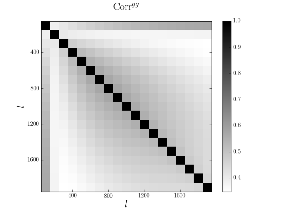
and computed using the same prescription as above. The computed correlation matrix for the galaxy autocorrelation is shown in Figure 2. It is clear that the non-Gaussian term has a non-negligible amplitude. However, in the cross-correlation covariance $\Sigma^{\kappa g}$, the noise reconstruction of the convergence map is very high, so the Gaussian term dominates the non-Gaussian one.

Figure 2: Correlation matrix $\mathrm{Corr}^{gg}$ built with the covariance of Equation (24) for the galaxy autocorrelation, using a binning of width $\delta l=100$ from $l_{min}=50$ to $l_{max}=1950$. The non-Gaussian term has a strong amplitude, contrary to the one in $\mathrm{Corr}^{\kappa\kappa}$ and $\mathrm{Corr}^{\kappa g}$ because of the very high noise reconstruction of the convergence $N_{l}^{\kappa\kappa}$.

2.3 The halo model

The halo model is based on the spherical collapse model (Gunn & Gott, 1972): large-scale structures formed from sufficiently overdense regions of space that collapsed under their own gravity. The remaining structures are called halos. Fitting formulaes for the number density of halos are presented in Section 2.3.1. Section 2.3.2 is about halo biasing with respect to dark matter; Section 2.3.3 presents the profiles of halos; and finally in Section 2.3.4, I compute the power spectrum and trispectrum in the halo model. For a thorough analysis of the halo model, see Cooray & Sheth (2002).

2.3.1 The number density of halos

A useful formula for the number density of halos at redshift $z$, $n\left(m,z\right)$ is provided by Sheth & Tormen (1999), following an original formula by Press & Schechter (1974):

$$\frac{m}{\bar{\rho}}n\left(m,z\right)dm=f\left(\nu\right)d\nu,$$ (29)

where $\bar{\rho}$ is the comoving density of the background with

$$f\left(\nu\right)=A\left(p\right)\left(1+\left(q\nu\right)^{-p}\right)\sqrt{\frac{q}{2\pi\nu}}e^{-q\nu/2},\quad\nu=\frac{\delta_{SC}^{2}}{\sigma^{2}\left(m,z\right)}.$$ (30)

In this formula, $A\left(p\right)\simeq 0.322$ such that $\intop f\left(\nu\right)d\nu=1$, $p\simeq 0.3$, $q\simeq 0.75$, $\delta_{SC}\simeq 1.68$ is the critical density required for spherical collapse, and

$$\sigma^{2}\left(m,z\right)=\int dk\frac{k^{2}P\left(k,z\right)}{2\pi^{2}}W\left(kR\right)^{2}$$ (31)

is the variance of the initial density field extrapolated to the present time using the linear prediction: $P\left(k,z\right)=\left(D^{+}\left(z\right)/D^{+}\left(0\right)\right)^{2}P\left(k,0\right)$. Here, $D^{+}$ is the linear growth factor, $R=\left(3m/4\pi\bar{\rho}\right)^{1/3}$ is the radius of a sphere of mean comoving density $\bar{\rho}$ enclosing a mass $m$, and $W$ is the Fourier transform of a top-hat function: $W\left(x\right)=3/x^{3}\left(\sin\left(x\right)-x\cos\left(x\right)\right)$. To compute the values of the linear power spectrum, I use the CAMB routines (Lewis & Bridle, 2002). The value $\nu=1$ defines a characteristic mass scale $m_{*}\simeq 4\times 10^{12}M_{\text{$\odot$}}/h$ at $z=0$.

In practice, owing to the limited range of integration ($v\apprge 10^{-2}$, otherwise the integration would bring unphysical values of the mass), the value of the parameter $A\left(p\right)$ is adapted to ensure that $\int f\left(\nu\right)d\nu=1$.

2.3.2 Halo biasing

Following Mo & White (1995) (see also Sheth & Tormen (1999) for an extension), the bias parameters of the overdensity of halos relative to the matter overdensity $\delta_{h}\left(\boldsymbol{x,}z;m\right)=\sum_{k>0}b_{k}\left(m,z\right)\delta\left(\boldsymbol{x}\right)^{k}/k!$ in the spherical collapse model (Gunn & Gott, 1972) are given by

$$b_{1}(m,z) = 1+\varepsilon_{1}+E_{1},$$

$$b_{2}(m,z) = 2(1+a_{2})(\varepsilon_{1}+E_{1})+\varepsilon_{2}+E_{2},$$

$$b_{3}\left(m,z\right) = 6\left(a_{2}+a_{3}\right)\left(\varepsilon_{1}+E_{1}\right)+3\left(1+2a_{2}\right)\left(\varepsilon_{2}+E_{2}\right)+\varepsilon_{3}+E_{3}$$ (32)

with

$$\varepsilon_{1} = \frac{q\nu-1}{\delta_{SC}},\quad\varepsilon_{2}=\frac{q\nu}{\delta_{SC}}\left(\frac{q\nu-3}{\delta_{SC}}\right),\quad\varepsilon_{3}=\frac{q\nu}{\delta_{SC}}\left(\frac{q\nu-3}{\delta_{SC}}\right)^{2}$$

$$E_{2} = \frac{2p}{\delta_{SC}\left(1+\left(q\nu\right)^{p}\right)},\quad\frac{E_{2}}{E_{1}}=\frac{1+2p}{\delta_{SC}}+2\varepsilon_{1},\quad\frac{E_{3}}{E_{1}}=\frac{4\left(p^{2}-1\right)+6pq\nu}{\delta_{SC}^{2}}+3\varepsilon_{1}^{2}$$

$$a_{2} = -17/21,\quad a_{3}=341/567.$$ (33)

These bias parameters obey the consistency relations

$$\int dm\frac{m}{\bar{\rho}}n\left(m,z\right)b_{k}\left(m,z\right)=\delta_{k1}^{K}.$$ (34)

Again, owing to the limited range of integration, the bias parameters are rescaled so as to ensure the consistency relations.

Within this framework, it is easy to compute the halo-halo correlations $P_{hh}$, $B_{hhh}$, and $T_{hhhh}$. The complete set of formulae for these correlations are given in Appendix A, with corrections that complete the formulae presented in Cooray & Sheth (2002).

2.3.3 Halo profiles

For the halo profile, I use a NFW profile (Navarro et al., 1997) given by

$$\rho\left(r;m\right)=\frac{\rho_{s}}{\left(r/r_{s}\right)\left(1+r/r_{s}\right)^{2}},$$ (35)

where $r_{s}=R_{vir}/c$, where $c$ is known as the concentration parameter, and $R_{vir}$ is the virialization radius defined by $4\pi R_{vir}^{3}\Delta\bar{\rho}/3=m$ with $\Delta\left(z\right)=\left(18\pi^{2}+82\left(\Omega_{m}\left(z\right)-1\right)-39\left(\Omega_{m}\left(z\right)-1\right)^{2}\right)/\Omega_{m}\left(z\right)$ given by the spherical collapse model (Bryan & Norman, 1998). The parameter $\rho_{s}$ is obtained by requesting that $m=\int d^{3}\boldsymbol{r}\rho\left(r;m\right)$. For the concentration parameter I use (Bullock et al., 2001)

$$c\left(m,z\right)=9\left(\frac{m}{m_{*}\left(z\right)}\right)^{-0.13}.$$ (36)

In what follows I use the Fourier transform of the normalized NFW profile $u\left(r;m\right)=\rho\left(r;m\right)/m$, which is

$$u\left(k;m\right) = \frac{4\pi\rho_{s}r_{s}^{3}}{m}\left\{\sin\left(kr_{s}\right)\left[\mathrm{Si}\left(\left[1+c\right]kr_{s}\right)-\mathrm{Si}\left(kr_{s}\right)\right]-\frac{\sin\left(ckr_{s}\right)}{\left(1+c\right)kr_{s}}\right.$$ (37)

$$+ \left.\cos\left(kr_{s}\right)\left[\mathrm{Ci}\left(\left[1+c\right]kr_{s}\right)-\mathrm{Ci}\left(kr_{s}\right)\right]\vphantom{\frac{\sin\left(ckr_{s}\right)}{\left(1+c\right)kr_{s}}}\right\},$$

where the sine and cosine integrals are

$$\mathrm{Ci}\left(x\right)=-\intop_{x}^{+\infty}\frac{\cos t}{t}dt\quad and\quad\mathrm{Si}\left(x\right)=\intop_{0}^{x}\frac{\sin t}{t}dt.$$ (38)

2.3.4 The power spectrum and trispectrum in the halo model

In this section I follow the formalism developed by Scherrer & Bertschinger (1991). The comoving dark matter density field is written as

$$\rho_{tot}\left(\boldsymbol{x}\right) = \sum_{i}\rho\left(\boldsymbol{x}-\boldsymbol{x_{i}},m_{i}\right)$$ (39)

$$\equiv \sum_{i}m_{i}u\left(\boldsymbol{x}-\boldsymbol{x_{i}}\right)$$

$$= \sum_{i}\int dmd^{3}\boldsymbol{x^{\prime}}\delta_{D}\left(m-m_{i}\right)\delta_{D}^{3}\left(\boldsymbol{x^{\prime}}-\boldsymbol{x_{i}}\right)m\,u\left(\boldsymbol{x}-\boldsymbol{x^{\prime}},\,m\right),$$

where the sum is performed over the halos $i$ and $\rho$ is the profile of a halo of mass $m_{i}$. The profile $u$ is defined such that $\int d^{3}\boldsymbol{x}u\left(\boldsymbol{x}\right)=1$. The number density of halos is

$$n\left(m\right)=\left\langle\sum_{i}\delta_{D}\left(m-m_{i}\right)\delta_{D}^{3}\left(\boldsymbol{x}-\boldsymbol{x_{i}}\right)\right\rangle,$$ (40)

such that

$$\bar{\rho}\equiv\left\langle\rho\left(\boldsymbol{x}\right)\right\rangle=\int mn\left(m\right)dm.$$ (41)

It is then straightforward to compute the power spectrum in this model. It can be split into two terms: the contributions coming from the same halo and the ones coming from two different halos:

$$P\left(k\right) = P^{1h}\left(k\right)+P^{2h}\left(k\right),\quad\mathrm{where}$$

$$P^{1h}\left(k\right) = M_{02}\left(k,k\right)$$

$$P^{2h}\left(k\right) = \left[M_{11}\left(k\right)\right]^{2}P^{PT}\left(k\right).$$ (42)

The power spectrum coming from two different halos is evaluated with Equation (56). In this equation, the linear power spectrum is used rather than the non-linear one. It is an approximation made so as not to overestimate the power spectrum on intermediate and small scales. On small scales, the one-halo term will dominate anyway. I have introduced the convenient notation:

$$M_{ij}\left(k_{1},...,k_{j}\right)=\intop dmn\left(m\right)b_{i}\left(m\right)\left(\frac{m}{\bar{\rho}}\right)^{j}u\left(k_{1};m\right)u\left(k_{2};m\right)...u\left(k_{j};m\right).$$ (43)

These coefficients depend only on the norm of the $k_{i}$. The trispectrum is evaluated in the same way. Since the entire formula is a bit long, it is given in Appendix A, with corrections to the formula given in Cooray & Hu (2001).

3 Data

3.1 Galaxy map

In this study, I use the galaxies from the CFHTLenS galaxy survey, a wide part of the Canada-France Hawaii Telescope Legacy Survey (CFHTLS), which consists in four fields centred at $2^{\mathrm{h}}18^{\mathrm{m}}00^{\mathrm{s}}$ $-07^{\mathrm{d}}00^{\mathrm{m}}00^{\mathrm{s}}$ for W1, $08^{\mathrm{h}}54^{\mathrm{m}}00^{\mathrm{s}}$ $-04^{\mathrm{d}}15^{\mathrm{m}}00^{\mathrm{s}}$ for W2, $14^{\mathrm{h}}17^{\mathrm{m}}54^{\mathrm{s}}$ $+54^{\mathrm{d}}30^{\mathrm{m}}31^{\mathrm{s}}$ for W3, and $22^{\mathrm{h}}13^{\mathrm{m}}18^{\mathrm{s}}$ $+01^{\mathrm{d}}19^{\mathrm{m}}00^{\mathrm{s}}$ for W4. Each has an area of $23-64\mathrm{\;deg^{2}}$, a total survey area of 154 $\mathrm{deg^{2}}$, and a depth in the $i_{AB}$ band of $i_{AB}=24.7$ (Heymans et al., 2012; Erben et al., 2013). The survey area was imaged using the Megaprime wide field imager mounted at the prime focus of the Canada-France-Hawaii Telescope (CFHT) and equipped with the MegaCam camera. MegaCam comprises an array of $9\times 4$ CCDs and has a field of view of 1 $\mathrm{deg^{2}}$.

I limit my analysis to galaxies in the redshift range $0.2<z<1.3$. These galaxies have been confirmed to have a photometric redshift distribution that resembles the measured spectroscopic redshift distribution (Heymans et al., 2012). Galaxies selected with $i_{AB}<24.5$ in this redshift slice have a scatter of $0.03<\sigma_{\Delta z}<0.06$ (where $\sigma_{\Delta z}^{2}$ is the variance in the difference between the photometric and spectroscopic redshifts $(z_{p}-z_{s})/(1+z_{s})$) with 10% of the galaxies classified as outliers (Benjamin et al., 2012). The reduction pipeline has been set to star_flag = 0 and $\mathrm{mask\leq 1}$ (description of each flag can be found in Erben et al. (2013)), and the magnitude cut to $18.0<i_{AB}<24.0$. The resulting catalogue has a number of galaxies $N_{gal}\simeq 6.58\times 10^{6}$ and a sky coverage of $f_{sky}\simeq 3.5\times 10^{-3}$. Table 1 sums up the catalogue parameters in each patch.

Patch	$N_{gal}$	$f_{sky}$	$\bar{n}\,\left(\mathrm{gal\,arcmin^{-1}}\right)$
All	$6.82\times 10^{6}$	$3.5\times 10^{-3}$	$15.1$
W1	$3.02\times 10^{6}$	$1.5\times 10^{-3}$	$15.0$
W2	$0.87\times 10^{6}$	$0.5\times 10^{-3}$	$14.8$
W3	$1.95\times 10^{6}$	$1.0\times 10^{-3}$	$15.3$
W4	$0.97\times 10^{6}$	$0.5\times 10^{-3}$	$15.3$

Table 1: CFHTLenS catalogue data

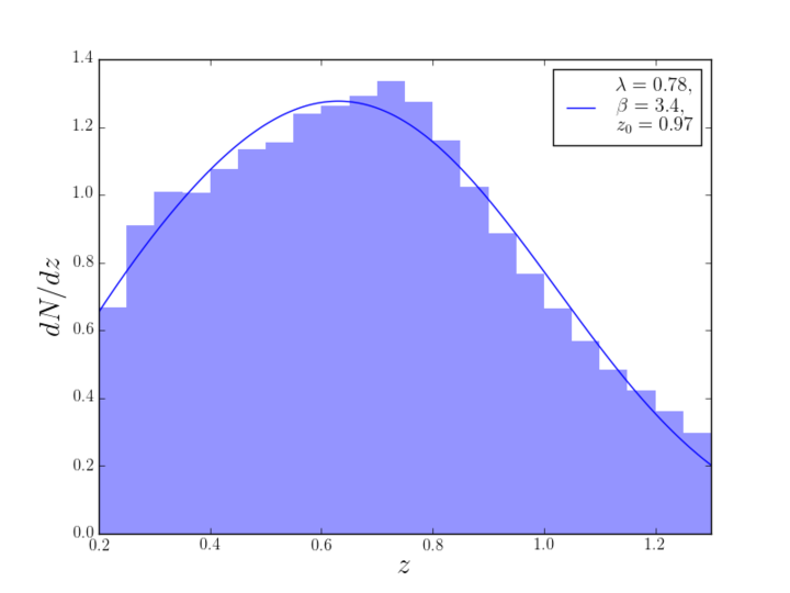
The redshift distribution $dN/dz$ used in Equation (5) is obtained by averaging the individual $P\left(z\right)$ of each galaxy in each redshift bin, ranging from $0.2<z<1.3$ with a bin size $\Delta z$ of $0.05$. This distribution is then fitted for analytic convenience with an incomplete gamma distribution, omitting the negligible error in redshift:

$$\frac{dN}{dz}=\frac{\alpha}{z_{0}}\left(\frac{z}{z_{0}}\right)^{\lambda}\exp\left(-\left(\frac{z}{z_{0}}\right)^{\beta}\right)$$ (44)

as shown in Figure 3. The best-fit values for the galaxy sample are $\lambda=0.78$, $\beta=3.4$, and $z_{0}=0.97$.

Figure 3: Redshift distribution of the CFHTLenS galaxies for all patches. The histogram is the recovered redshift distribution obtained by averaging the individual $P\left(z\right)$ and the solid line represents the best-fit using Equation (44). The best-fit values of $\lambda$, $\beta$, and $z_{0}$ are used in Equation (5) for $W^{g}$.

The galaxy overdensity is computed as a HEALPix map (Górski et al., 2005) with $N_{side}=2048$ (corresponding to a pixel size of $\sim 1.^{\prime}7$) by

$$\delta_{i}=\frac{N_{i}/w_{i}-\left\langle N\right\rangle}{\left\langle N\right\rangle},$$ (45)

where $w_{i}=S_{i}^{u}/S_{i}$ is the ratio between the unmasked surface of a HEALPix pixel and the total suface of this pixel, $N_{i}$ is the number of galaxies counted in a pixel, and $\left\langle N\right\rangle=\left(\sum_{i}N_{i}/w_{i}\right)/N_{pix}$ is the mean number of galaxies per pixel, corresponding to a number density of $\bar{n}=15.1$ galaxies per square arcminute.

3.2 Convergence map

I use the observed and simulated convergence map from the Planck 2015 release (Collaboration et al., 2015) and compare the results with the 2013 release (Planck Collaboration et al., 2014). The 2015 map is produced by applying a quadratic estimator to all nine frequency bands with a galaxy and point-source mask, leaving a total of 67.3% of the sky for analysis. The 2013 map is obtained by combining only the 143 and 217 GHz channels. The 2015 map is released as a $\kappa_{lm}$ map for $8\leq l\leq 2048$, while the 2013 map is a $\bar{\phi}$ map and so is transformed into a convergence map by taking the transform

$$\kappa_{lm}=\frac{1}{R_{l}^{\phi\phi}}\frac{l\left(l+1\right)}{2}\bar{\phi}_{lm}$$ (46)

where $R_{l}^{\phi\phi}$ is a normalization factor explained in Planck Collaboration et al. (2014). The 2013 and 2015 masks are combined for consistency. The final mask for the cross-correlation is obtained by multiplying the convergence mask and the galaxy mask, then applied by converting the convergence multi-poles $\kappa_{lm}$ in real space and multiplying with the mask.

The noise for the auto-correlation has been estimated from the set of 100 simulated lensing maps released by the Planck team. The noise power spectrum $N_{l}^{\kappa\kappa}$ was estimated by averaging over the 100 simulations the autospectrum of the masked difference map between the reconstructed and the input lensing map.

4 Constraints on galaxy bias and cross-correlation amplitude

Following Planck Collaboration et al. (2014) and Collaboration et al. (2015), I introduce a new parameter, $A$, named the lensing amplitude, that scales the amplitude of the cross-correlation: $\tilde{C}_{l_{i}}^{\kappa g}=AC_{l_{i}}^{\kappa g}\left(b\right)$. Its expected value is obviously one. I then use the combined cross- and auto-correlation to constrain the galaxy bias $b$ and the lensing amplitude $A$.

I use the following scheme, developed by e.g. Bianchini et al. (2015) : the cross and auto-correlation are organized in a single vector following

$$\boldsymbol{C}=\left(\boldsymbol{C}^{\kappa g},\boldsymbol{C}^{gg}\right)$$ (47)

where $\boldsymbol{C}^{XY}$ is the vector containing $\left(C_{l_{i}}^{XY}\right)^{i=1..N_{bin}}$ in the $N_{bin}=19$ bins used. The total covariance matrix writes as

$$\Sigma=\left(\begin{array}[]{cc}\Sigma^{\kappa g}&\left(\Sigma^{\kappa g-gg}\right)^{T}\\ \Sigma^{\kappa g-gg}&\Sigma^{gg}\end{array}\right),$$ (48)

where the mixed covariance $\Sigma_{ij}^{\kappa g-gg}$ is defined in Equation (28). The covariances are evaluated for the fiducial values $A=1$ and $b=1$. According to Bayes’ theorem, the posterior probability of a given set of parameters $\left(A,b\right)$ given the data $\boldsymbol{C}$, is

$$P\left(A,b\mid\boldsymbol{C}\right)=\frac{P\left(A,b\right)P\left(\boldsymbol{C}\mid A,b\right)}{P\left(\boldsymbol{C}\right)}$$ (49)

where $P\left(A,b\right)$ is the prior on the parameters, $P\left(\boldsymbol{C}\mid A,b\right)$ is the likelihood function for measuring $\boldsymbol{C}$ given $A,b$, and $P\left(\boldsymbol{C}\right)$ is a normalization factor. I assume a Gaussian likelihood function, which takes the form

$$P\left(\boldsymbol{C}\mid A,b\right)=\frac{1}{\sqrt{\left(2\pi\right)^{2N_{bin}}\det\left(\Sigma\right)}}\exp\left\{-\frac{1}{2}\left(\tilde{\boldsymbol{C}}-\boldsymbol{C}\left(A,b\right)\right)\Sigma^{-1}\left(\tilde{\boldsymbol{C}}-\boldsymbol{C}\left(A,b\right)\right)\right\},$$ (50)

and a flat prior. To sample the parameter space, I use a Monte-Carlo Markov Chain (MCMC) method employing the Python module EMCEE (Foreman-Mackey et al., 2013), which is a public implementation of the affine invariant MCMC ensemble sampler (Goodman & Weare, 2010). The resulting parameters are estimated by the median of the posterior distribution after marginalizing over the other parameters with uncertainties given by the $16^{th}$ and $84^{th}$ percentiles. For a Gaussian distribution, the median is equal to the maximum likelihood value, and the percentiles correspond to the $-1\sigma$ and $+1\sigma$ error bars; here, the recovered distributions are very close to Gaussians.

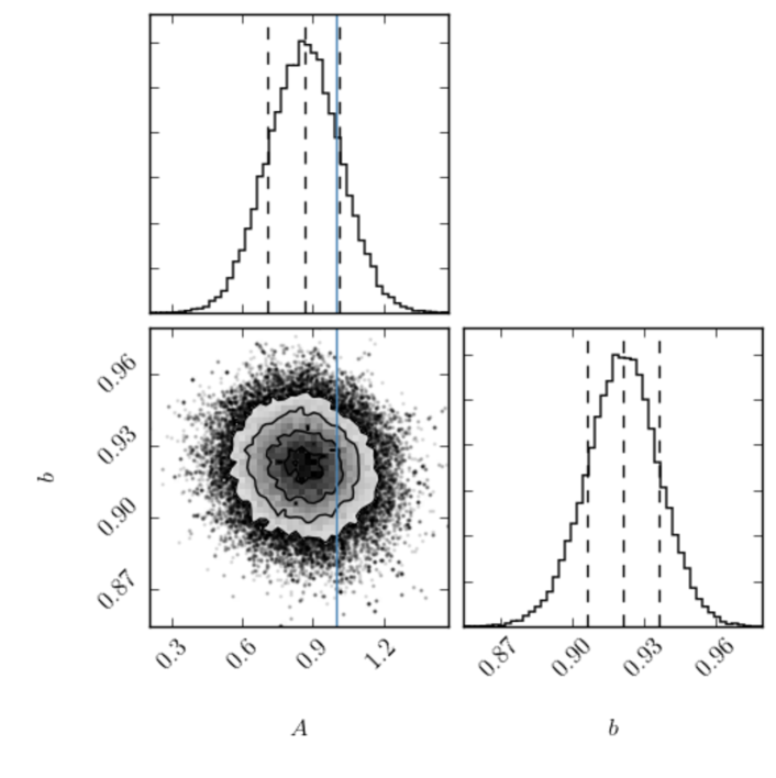
The two-dimensional posterior distribution and the marginalized ones are shown in Figure 4 for the 2013 release, and in Figure 5 for the 2015 release, using all the patches together. Table 2 sums up the values of parameters $A$ and $b$ for each patch and for the two releases with $1\sigma$ error bars, together with the $\chi^{2}$ calculated as $\chi^{2}=\left(\tilde{\boldsymbol{C}}-\boldsymbol{C}\left(A,b\right)\right)\Sigma^{-1}\left(\tilde{\boldsymbol{C}}-\boldsymbol{C}\left(A,b\right)\right)$ for $\nu=2N_{bin}-2$ degrees of freedom. Parameter $b$ is mostly constrained by the galaxy auto-correlation, so it has approximately the same value for the two releases.

Figure 4: Posterior distribution in the $A-b$ plane, together with the marginalized distributions for each parameter, for the 2013 data. The contours show the $0.5\sigma$, $1\sigma$, $1.5\sigma$, and $2\sigma$ lines from the centre to the border. The solid red line represents the fiducial value $A=1$, and the dashed lines the $-1\sigma$ and $+1\sigma$ error bars.

Figure 5: Same plot as in Figure 4, but for the 2015 data.

		2013			2015
Patch	$A$	$b$	$\chi^{2}/\nu$	$A$	$b$	$\chi^{2}/\nu$
All	$1.05_{-0.15}^{+0.15}$	$0.93_{-0.02}^{+0.02}$	$47.2/36$	$0.86_{-0.16}^{+0.15}$	$0.92_{-0.02}^{+0.02}$	$37.4/36$
W1	$0.69_{-0.22}^{+0.23}$	$0.90_{-0.02}^{+0.02}$	$54.3/36$	$0.41_{-0.24}^{+0.24}$	$0.89_{-0.03}^{+0.02}$	$48.2/36$
W2	$1.29_{-0.34}^{+0.34}$	$1.04_{-0.04}^{+0.04}$	$29.0/36$	$1.22_{-0.36}^{+0.35}$	$1.03_{-0.04}^{+0.04}$	$30.9/36$
W3	$1.34_{-0.28}^{+0.28}$	$0.94_{-0.03}^{+0.03}$	$50.9/36$	$0.99_{-0.29}^{+0.29}$	$0.92_{-0.03}^{+0.03}$	$39.6/36$
W4	$1.28_{-0.40}^{+0.40}$	$0.89_{-0.04}^{+0.04}$	$44.1/36$	$1.60_{-0.40}^{+0.42}$	$0.88_{-0.04}^{+0.04}$	$59.1/36$

Table 2: Best-fit values for $A$ and $b$ using both cross- and auto-correlation for the 2013 and 2015 releases.

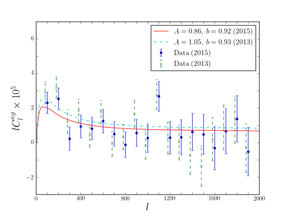
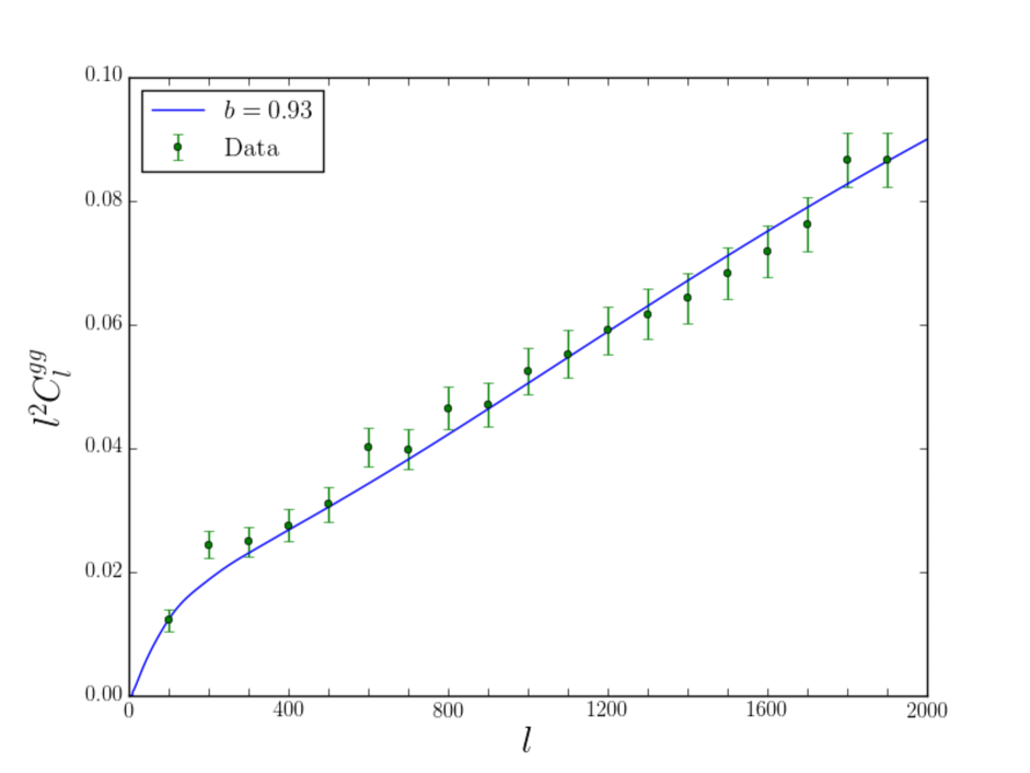
The cross- and auto-correlations, together with the best-fit parameters theoretical prediction (with all patches together), are shown in Figures 6 and 7.

Figure 6: CMB convergence - galaxy over-density cross-correlation $C_{l}^{\kappa g}$ using all patches. Error bars are computed from the theoretical correlation matrix of Equation (24). The solid line and the solid blue points are the 2015 best-fit and the 2015 data, respectively, while the dashed line and the dashed green points are the 2013 best-fit and the 2013 data.

Figure 7: As in Figure 6, but for the galaxy auto-correlation $C_{l}^{gg}$ using all patches. The solid line is the best fit of 2013 and 2015 (which give the same value for $b$), and the data are shown in green.

5 Consistency checks

5.1 Simulations

To validate the algorithm employed to reconstruct the convergence and galaxy maps and to check the consistency of the theoretical error bars in the Gaussian limit, I created $N_{sim}=100$ simulations of the galaxy and convergence maps. I used the Healpy synfast function to generate a set of $\kappa_{lm}$ and $g_{lm}$ and the theoretical $C_{l}^{\kappa\kappa}$, $C_{l}^{\kappa g}$, and $C_{l}^{gg}$ given in Equations (12), (7), and (13), with $b=1$. The multi-pole coefficients are synthetized by

$$\kappa_{lm} = \xi_{1}\left(C_{l}^{\kappa\kappa}\right)^{1/2}$$

$$g_{lm} = \xi_{1}\frac{C_{l}^{\kappa g}}{\left(C_{l}^{\kappa\kappa}\right)^{1/2}}+\xi_{2}\left(C_{l}^{gg}-\frac{\left(C_{l}^{\kappa g}\right)^{2}}{C_{l}^{\kappa\kappa}}\right)^{2},$$ (51)

where for each value of $l$ and $m>0$, $\xi_{1}$ and $\xi_{2}$ are two complex numbers drawn from a Gaussian distribution of mean $0$ and variance $1$, whereas for $m=0$ they are real.

To account for the level of noise in the maps, I replaced $C_{l}^{\kappa\kappa}$ by $C_{l}^{\kappa\kappa}+N_{l}^{\kappa\kappa}$ with $N_{l}^{\kappa\kappa}$ the noise given in the Planck Collaboration release. As pointed out by the Planck 2013 Wiki, this noise is not accurate enough for the auto-correlation, but it should be sufficient for the cross-correlation, which is not biased by this noise term. The noise in the galaxy map was accounted for by drawing the number of galaxies in each pixel from a Poisson distribution with mean

$$\lambda\left(\boldsymbol{\theta}\right)=\left\langle N\right\rangle\left(1+\delta\left(\boldsymbol{\theta}\right)\right)$$ (52)

where $\left\langle N\right\rangle$ is the mean number of galaxies per pixel of the original map, and $\delta\left(\boldsymbol{\theta}\right)$ the simulated overdensity map. I then replaced the galaxy number count $N_{i}/w_{i}$ in Equation 45 by $\lambda\left(\boldsymbol{\theta}\right)$. The Poisson noise of variance $N_{l}^{gg}=1/\bar{n}$ was thus included in this map with $\bar{n}$ the number of galaxies per steradian.

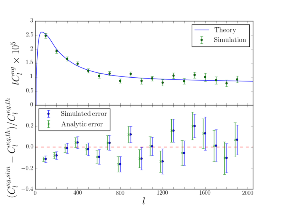
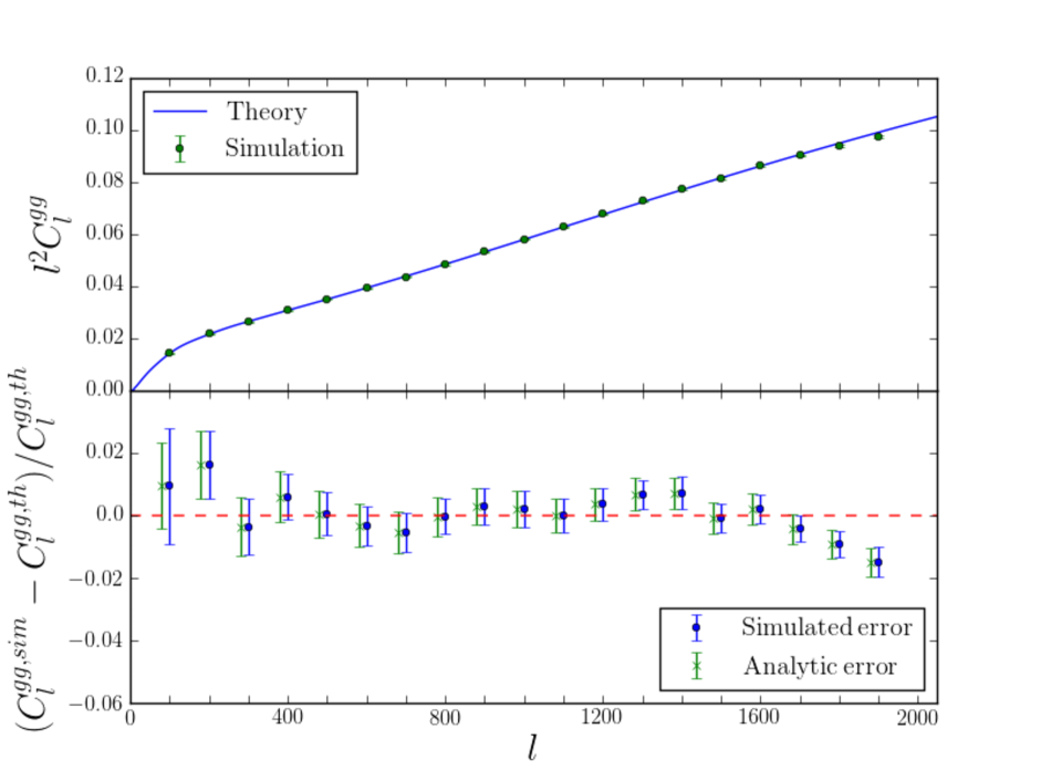
I then applied the spectral estimators described in the previous sections to the simulated convergence and over-density maps. The recovered $C_{l}^{\kappa g}$ and $C_{l}^{gg}$ averaged over the 100 simulations are shown in Figs. 8 and 9. The mean correlation was computed as

$$\left\langle\tilde{C}_{l_{i}}^{XY}\right\rangle=\frac{1}{N_{sim}}\sum_{\alpha=1}^{N_{sim}}\tilde{C}_{l_{i}}^{XY,\alpha}$$ (53)

where $X,Y=\left\{\kappa,g\right\}$, $\alpha$ is the number of the simulation, and $i$ refers to the bin in $l$ of width $\delta l=100$. The covariance matrix of the samples was computed as

$$\tilde{\Sigma}_{ij}^{XY}=\frac{1}{N_{sim}-1}\sum_{\alpha=1}^{N_{sim}}\left(\tilde{C}_{l_{i}}^{XY,\alpha}-\left\langle\tilde{C}_{l_{i}}^{XY}\right\rangle\right)\left(\tilde{C}_{l_{j}}^{XY,\alpha}-\left\langle\tilde{C}_{l_{j}}^{XY}\right\rangle\right).$$ (54)

For comparison, I show the theoretical error bars and the recovered simulated error bars for the mean correlation computed as

$$\Delta\tilde{C}_{l_{i}}^{XY}=\left(\frac{\tilde{\Sigma}_{ii}^{XY}}{N_{sim}}\right)^{1/2}$$ (55)

with the same formula for the theoretical error bars, using only the Gaussian term in Equation (24) because the simulations are Gaussian. They are in very good agreement.

Figure 8: Upper panel: Cross-correlation of the simulated galaxy and lensing maps using $b=1$. The solid line represents the input cross-correlation, and the points represent the reconstructed cross-correlation averaged over $N_{sim}=100$ simulations, together with the simulated error bars.
Lower panel: Fractional difference between the input and the recovered cross-correlations. The blue error bars are recovered from the simulations using Equation (54) for the covariance matrix, and the red ones are analytic using Equation (24) for the covariance, keeping only the Gaussian term.

Figure 9: Same plot as Figure (8), but for $C_{l}^{gg}$.

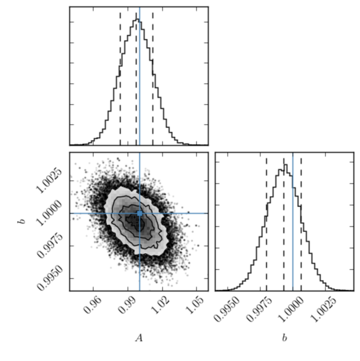
I also fitted a galaxy bias and a lensing amplitude following the pipeline explained in Section 4 and compared them to the fiducial values used in the simulations $A=1$ and $b=1$. To this aim I replaced the correlations $C_{l_{i}}^{XY}$ by the mean correlations $\left\langle\tilde{C}_{l_{i}}^{XY}\right\rangle$ and the covariances matrices $\Sigma^{XY}$ by the mean correlation covariance $\tilde{\Sigma}^{XY}/N_{sim}$. The fitted values of the parameters are $A=0.998_{-0.014}^{+0.014}$ and $b=0.999_{-0.001}^{+0.001}$, indicating that the reconstruction is good. Figure 10 shows a corner plot of the MCMC sampler for the simulations, as in Figure 4.

Figure 10: As in Figure 4, but for the Gaussian simulations. The horizontal and vertical solid lines show the fiducial values $A=1$ and $b=1$ used in the simulations.

5.2 Null tests

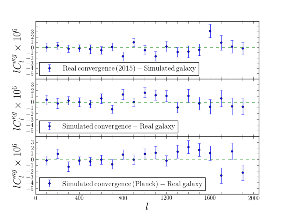
To check that there is no systematics in the pipeline descibed above, I performed a series of null tests consisting in cross-correlating a real map with the $N_{sim}=100$ simulated maps of Section 5.1, both for a real convergence map with a simulated galaxy map and for a simulated convergence map with a real galaxy map, using all the patches together. The expected signal is of null amplitude, with a simulated covariance given by Equation (54) applied to the null test simulations. As shown in Figure 11, in both cases no significant signal was detected. The fitted values of the product $A\times b$ (which is the amplitude of the cross-correlation) are summarized in Table 3.

To validate the use of Gaussian simulations in the computation of covariances, I also cross-correlated the 100 simulated Planck maps given by the Planck collaboration with the real galaxy overdensity field. I obtain a result similar to the Gaussian simulation null test for the error bars, indicating that the use of Gaussian simulations is relevant.

Figure 11: Upper panel: Mean correlation between the true lensing map of 2015 and 100 simulated galaxy maps using all patches.
Middle panel: Mean correlation between the true galaxy map using all patches and 100 gaussian simulated lensing maps.
Lower panel: Mean correlation between the true galaxy map using all patches and 100 Planck simulated lensing maps.
In all cases the signal is consistent with no correlation.

Null test	$A\times b$	$\chi^{2}/\nu$
2013 Real convergence - Simulated galaxy	$-0.013_{-0.018}^{+0.018}$	$24.8/19$
2015 Real convergence - Simulated Galaxy	$-0.001_{-0.018}^{+0.017}$	$21.0/19$
Simulated convergence - Real galaxy	$0.015_{-0.016}^{+0.016}$	$21.5/19$
Simulated convergence (Planck) - Real galaxy	$0.003_{-0.014}^{+0.014}$	$25.3/19$

Table 3: Null tests performed as explained in Section 5.2.

6 Summary and conclusions

I have presented the results from a joint analysis of the cross and auto-correlation of the CFHTLenS galaxy catalogue and Planck CMB lensing, checking the reliability of my result by null tests and Gaussian simulations. I found a galaxy bias of $b=0.92_{-0.02}^{+0.02}$ and a cross-correlation amplitude of $A=0.86_{-0.15}^{+0.15}$ for the 2015 release, whereas for the 2013 release I found $b=0.93_{-0.02}^{+0.02}$ and $A=1.05_{-0.15}^{+0.15}$. This confirms the difference between the two releases shown by Omori & Holder (2015), but the trend is less clear, and both results are compatible with each other. These results are consistent with the amplitudes obtained from the Planck lensing autocorrelation in Collaboration et al. (2015): $A=0.987\pm 0.025$ for the 2015 release and $A=1.005\pm 0.043$ for the 2013 release. The value of the galaxy bias suggests that galaxies in this magnitude range are unbiased tracers of dark matter.

This study suggests that the joint analysis of the cross and auto-correlation can put strong constraints on the properties of tracers of dark matter. Forthcoming wide galaxy surveys probing fainter magnitudes will improve the constraining power of this kind of study, both by a larger survey area to improve statistics and a sufficient galaxy number density to avoid shot noise. They are expected to put better constraints on the cosmological model used in this paper.

Appendix A The halo model power spectrum, bispectrum, and trispectrum

Using the bias parameters given in Section 2.3.2, the halo-halo correlations are (the dependence on $z$ is omitted for clarity, along with the $k$’s and $m$’s when not needed):

$$P_{hh} = b_{1}\left(m_{1}\right)b_{1}\left(m_{2}\right)P^{PT}\left(k\right),$$

$$B_{hhh} = b_{1}\left(m_{1}\right)b_{1}\left(m_{2}\right)b_{1}\left(m_{3}\right)B^{PT}+\left[b_{2}\left(m_{1}\right)b_{1}\left(m_{2}\right)b_{1}\left(m_{3}\right)P^{PT}\left(k_{2}\right)P^{PT}\left(k_{3}\right)+cyc.\right],$$

$$T_{hhhh} = b_{1}\left(m_{1}\right)b_{1}\left(m_{2}\right)b_{1}\left(m_{3}\right)b_{1}\left(m_{4}\right)T^{PT}$$ (56)

$$+ b_{3}\left(m_{1}\right)b_{1}\left(m_{2}\right)b_{1}\left(m_{3}\right)b_{1}\left(m_{4}\right)P^{PT}\left(k_{2}\right)P^{PT}\left(k_{3}\right)P^{PT}\left(k_{4}\right)+cyc.$$

$$+ b_{2}\left(m_{1}\right)b_{1}\left(m_{2}\right)b_{1}\left(m_{3}\right)b_{1}\left(m_{4}\right)\left[P^{PT}\left(k_{2}\right)B^{PT}\left(\boldsymbol{k_{1}}+\boldsymbol{k_{2}},\boldsymbol{k_{3}},\boldsymbol{k_{4}}\right)+\left(2\leftrightarrow 3\right)+\left(2\leftrightarrow 4\right)\right]+cyc.$$

$$+ b_{2}\left(m_{1}\right)b_{1}\left(m_{3}\right)b_{1}\left(m_{4}\right)\left\{b_{2}\left(m_{2}\right)P^{PT}\left(k_{3}\right)P^{PT}\left(k_{4}\right)\left[P^{PT}\left(\left|\boldsymbol{k_{1}}+\boldsymbol{k_{3}}\right|\right)+P^{PT}\left(\left|\boldsymbol{k_{1}}+\boldsymbol{k_{4}}\right|\right)\right]\right.$$

$$\hphantom{b_{2}\left(m_{1}\right)b_{1}\left(m_{3}\right)b_{1}\left(m_{4}\right)}\left.+\left(2\leftrightarrow 3\right)+\left(2\leftrightarrow 4\right)\vphantom{P^{PT}\left(\left|\boldsymbol{k_{1}}+\boldsymbol{k_{3}}\right|\right)}\right\}+cyc.$$

The formula given in Cooray & Sheth (2002) (Equation (90)) for the trispectrum is actually incomplete. Here, $P^{PT}$, $B^{PT}$ and $T^{PT}$ are the power spectrum, bispectrum, and trispectrum at lowest order in perturbation theory (see Bernardeau et al. (2002) for a review) given by

$$B^{PT}\left(\boldsymbol{k_{1}},\boldsymbol{k_{2}},\boldsymbol{k_{3}}\right) = 2F_{2}^{s}\left(\boldsymbol{k_{1}},\boldsymbol{k_{2}}\right)P^{PT}\left(k_{1}\right)P^{PT}\left(k_{2}\right)+\left(\boldsymbol{k_{1}}\leftrightarrow\boldsymbol{k_{3}}\right)+\left(\boldsymbol{k_{2}}\leftrightarrow\boldsymbol{k_{3}}\right)$$

$$T^{PT}\left(\boldsymbol{k_{1}},-\boldsymbol{k_{1}},\boldsymbol{k_{2}},-\boldsymbol{k_{2}}\right) = 4P^{PT}\left(\boldsymbol{k_{1}}+\boldsymbol{k_{2}}\right)\left[F_{2}^{s}\left(-\boldsymbol{k_{1}},\boldsymbol{k_{1}}+\boldsymbol{k_{2}}\right)P^{PT}\left(k_{1}\right)+\left(\boldsymbol{k_{1}}\leftrightarrow\boldsymbol{k_{2}}\right)\right]+\left(\boldsymbol{k_{1}}\leftrightarrow-\boldsymbol{k_{1}}\right)$$ (57)

$$+ 12\left[F_{3}^{s}\left(\boldsymbol{k_{1}},-\boldsymbol{k_{1}},\boldsymbol{k_{2}}\right)P^{PT}\left(k_{1}\right)^{2}P^{PT}\left(k_{2}\right)+\left(\boldsymbol{k_{1}}\leftrightarrow\boldsymbol{k_{2}}\right)\right]$$

where the symmetrized kernels $F_{n}^{s}$ are derived in Goroff et al. (1986). There is a very small dependence of the kernels on the parameter $\Omega_{m}$, which is ignored in this study.

The halo model power spectrum and trispectrum are then computed as (using the notation $M_{ij}\left(k_{1},...,k_{j}\right)$ given in Equation (43)):

$$P\left(k\right) = P^{1h}\left(k\right)+P^{2h}\left(k\right),\quad\mathrm{where}$$

$$P^{1h}\left(k\right) = M_{02}\left(k,k\right)$$

$$P^{2h}\left(k\right) = \left[M_{11}\left(k\right)\right]^{2}P^{PT}\left(k\right).$$ (58)

Since I only need terms of the form $T\left(\boldsymbol{k_{1}},-\boldsymbol{k_{1}},\boldsymbol{k_{2}},-\boldsymbol{k_{2}}\right)$ (see Equation (25)), the trispectrum can be simplified as

$$T_{hhhh}\left(\boldsymbol{k_{1}},-\boldsymbol{k_{1}},\boldsymbol{k_{2}},-\boldsymbol{k_{2}}\right) = T^{1h}+T^{2h}+T^{3h}+T^{4h}$$ (59)

with

$$T^{1h} = M_{04}\left(k_{1},k_{1},k_{2},k_{2}\right)$$

$$T^{2h} = 2M_{11}\left(k_{1}\right)M_{13}\left(k_{1},k_{2},k_{2}\right)P^{PT}\left(k_{1}\right)+\left(k_{1}\leftrightarrow k_{2}\right)$$

$$+ M_{12}\left(k_{1},k_{2}\right)^{2}\left[P^{PT}\left(\left|\boldsymbol{k_{1}}+\boldsymbol{k_{2}}\right|\right)+\left(\boldsymbol{k_{1}}\leftrightarrow-\boldsymbol{k_{1}}\right)\right]$$

$$T^{3h} = 2M_{11}\left(k_{1}\right)M_{11}\left(k_{2}\right)M_{12}\left(k_{1},k_{2}\right)\left[B^{PT}\left(\boldsymbol{k_{1}},\boldsymbol{k_{2}},-\boldsymbol{k_{1}}-\boldsymbol{k_{2}}\right)+\left(\boldsymbol{k_{1}}\leftrightarrow-\boldsymbol{k_{1}}\right)\right]$$

$$+ M_{11}\left(k_{1}\right)^{2}M_{22}\left(k_{2},k_{2}\right)P^{PT}\left(k_{1}\right)^{2}+\left(k_{1}\leftrightarrow k_{2}\right)$$

$$+ 4M_{11}\left(k_{1}\right)M_{11}\left(k_{2}\right)M_{22}\left(k_{1},k_{2}\right)P^{PT}\left(k_{1}\right)P^{PT}\left(k_{2}\right)$$

$$+ 2M_{12}\left(k_{1},k_{2}\right)\left[P^{PT}\left(\left|\boldsymbol{k_{1}}+\boldsymbol{k_{2}}\right|\right)+\left(\boldsymbol{k_{1}}\leftrightarrow-\boldsymbol{k_{1}}\right)\right]\left[M_{21}\left(k_{1}\right)M_{11}\left(k_{2}\right)P^{PT}\left(k_{2}\right)+\left(k_{1}\leftrightarrow k_{2}\right)\right]$$

$$T^{4h} = M_{11}\left(k_{1}\right)^{2}M_{11}\left(k_{2}\right)^{2}T^{PT}\left(\boldsymbol{k_{1}},-\boldsymbol{k_{1}},\boldsymbol{k_{2}},-\boldsymbol{k_{2}}\right)$$ (60)

$$+ 2M_{31}\left(k_{1}\right)M_{11}\left(k_{1}\right)M_{11}\left(k_{2}\right)^{2}P^{PT}\left(k_{1}\right)P^{PT}\left(k_{2}\right)^{2}+\left(k_{1}\leftrightarrow k_{2}\right)$$

$$+ 2M_{21}\left(k_{1}\right)M_{11}\left(k_{1}\right)M_{11}\left(k_{2}\right)^{2}P^{PT}\left(k_{2}\right)\left[B^{PT}\left(\boldsymbol{k_{1}},\boldsymbol{k_{2}},-\boldsymbol{k_{1}}-\boldsymbol{k_{2}}\right)+\left(\boldsymbol{k_{1}}\leftrightarrow-\boldsymbol{k_{1}}\right)\right]+\left(k_{1}\leftrightarrow k_{2}\right)$$

$$+ 2M_{21}\left(k_{1}\right)M_{11}\left(k_{2}\right)P^{PT}\left(k_{2}\right)\left[M_{21}\left(k_{1}\right)M_{11}\left(k_{2}\right)P^{PT}\left(k_{2}\right)+M_{11}\left(k_{1}\right)M_{21}\left(k_{2}\right)P^{PT}\left(k_{1}\right)\right]$$

$$\hphantom{2M_{21}\left(k_{1}\right)M_{11}\left(k_{2}\right)P^{PT}\left(k_{2}\right)}\times\left[P^{PT}\left(\left|\boldsymbol{k_{1}}+\boldsymbol{k_{2}}\right|\right)+P^{PT}\left(\left|\boldsymbol{k_{1}}-\boldsymbol{k_{2}}\right|\right)\right]+\left(k_{1}\leftrightarrow k_{2}\right).$$

This formula corrects the one of Cooray & Hu (2001), which is incomplete for both the three-halo and four-halo terms.

A code implementation in Python computing this trispectrum in the halo model is available upon request to the author.

References

• Benjamin et al. (2012) Benjamin, J., Van Waerbeke, L., Heymans, C., et al. 2012, arXiv:1212.3327 [astro-ph], arXiv: 1212.3327
• Bernardeau et al. (2002) Bernardeau, F., Colombi, S., Gaztanaga, E., & Scoccimarro, R. 2002, Physics Reports, 367, 1, arXiv: astro-ph/0112551
• Bernardeau et al. (2010) Bernardeau, F., Pitrou, C., & Uzan, J.-P. 2010, arXiv:1012.2652 [astro-ph, physics:gr-qc], arXiv: 1012.2652
• Bianchini et al. (2015) Bianchini, F., Bielewicz, P., Lapi, A., et al. 2015, The Astrophysical Journal, 802, 64, arXiv: 1410.4502
• Bleem et al. (2012) Bleem, L. E., van Engelen, A., Holder, G. P., et al. 2012, The Astrophysical Journal, 753, L9, arXiv: 1203.4808
• Bryan & Norman (1998) Bryan, G. L. & Norman, M. L. 1998, The Astrophysical Journal, 495, 80, arXiv: astro-ph/9710107
• Bullock et al. (2001) Bullock, J. S., Kolatt, T. S., Sigad, Y., et al. 2001, Monthly Notices of the Royal Astronomical Society, 321, 559, arXiv: astro-ph/9908159
• Collaboration et al. (2015) Collaboration, P., Ade, P. A. R., Aghanim, N., et al. 2015, arXiv:1502.01591 [astro-ph], arXiv: 1502.01591
• Cooray & Hu (2001) Cooray, A. & Hu, W. 2001, The Astrophysical Journal, 554, 56, arXiv: astro-ph/0012087
• Cooray & Sheth (2002) Cooray, A. & Sheth, R. 2002, Physics Reports, 372, 1, arXiv: astro-ph/0206508
• Erben et al. (2013) Erben, T., Hildebrandt, H., Miller, L., et al. 2013, Monthly Notices of the Royal Astronomical Society, 433, 2545
• Foreman-Mackey et al. (2013) Foreman-Mackey, D., Hogg, D. W., Lang, D., & Goodman, J. 2013, Publications of the Astronomical Society of the Pacific, 125, 306, arXiv: 1202.3665
• Geach et al. (2013) Geach, J. E., Hickox, R. C., Bleem, L. E., et al. 2013, The Astrophysical Journal, 776, L41
• Goodman & Weare (2010) Goodman, J. & Weare, J. 2010, Communications in Applied Mathematics and Computational Science, 5, 65
• Goroff et al. (1986) Goroff, M. H., Grinstein, B., Rey, S.-J., & Wise, M. B. 1986, The Astrophysical Journal, 311, 6
• Górski et al. (2005) Górski, K. M., Hivon, E., Banday, A. J., et al. 2005, The Astrophysical Journal, 622, 759
• Gunn & Gott (1972) Gunn, J. E. & Gott, III, J. R. 1972, The Astrophysical Journal, 176, 1
• Heymans et al. (2012) Heymans, C., Van Waerbeke, L., Miller, L., et al. 2012, Monthly Notices of the Royal Astronomical Society, 427, 146
• Hirata et al. (2008) Hirata, C. M., Ho, S., Padmanabhan, N., Seljak, U., & Bahcall, N. 2008, Physical Review D, 78, arXiv: 0801.0644
• Lewis & Bridle (2002) Lewis, A. & Bridle, S. 2002, Physical Review D, 66, 103511
• LoVerde & Afshordi (2008) LoVerde, M. & Afshordi, N. 2008, Physical Review D, 78, arXiv: 0809.5112
• Mo & White (1995) Mo, H. J. & White, S. D. M. 1995, arXiv:astro-ph/9512127, arXiv: astro-ph/9512127
• Moessner et al. (1998) Moessner, R., Jain, B., & Villumsen, J. V. 1998, Monthly Notices of the Royal Astronomical Society, 294, 291, arXiv: astro-ph/9708271
• Navarro et al. (1997) Navarro, J. F., Frenk, C. S., & White, S. D. M. 1997, The Astrophysical Journal, 490, 493, arXiv: astro-ph/9611107
• Okamoto & Hu (2003) Okamoto, T. & Hu, W. 2003, Physical Review D, 67, arXiv: astro-ph/0301031
• Omori & Holder (2015) Omori, Y. & Holder, G. 2015, arXiv:1502.03405 [astro-ph], arXiv: 1502.03405
• Peter & Uzan (2013) Peter, P. & Uzan, J.-P. 2013, Primordial cosmology, 1st edn., Oxford graduate texts (Oxford: Oxford Univ. Press)
• Planck Collaboration et al. (2014) Planck Collaboration, Ade, P. A. R., Aghanim, N., et al. 2014, Astronomy & Astrophysics, 571, A17
• Press & Schechter (1974) Press, W. H. & Schechter, P. 1974, The Astrophysical Journal, 187, 425
• Scherrer & Bertschinger (1991) Scherrer, R. J. & Bertschinger, E. 1991, The Astrophysical Journal, 381, 349
• Sherwin et al. (2012) Sherwin, B. D., Das, S., Hajian, A., et al. 2012, Physical Review D, 86, arXiv: 1207.4543
• Sheth & Tormen (1999) Sheth, R. K. & Tormen, G. 1999, Monthly Notices of the Royal Astronomical Society, 308, 119
• Smith et al. (2007) Smith, K. M., Zahn, O., & Dore, O. 2007, Physical Review D, 76, arXiv: 0705.3980
• Takada & Hu (2013) Takada, M. & Hu, W. 2013, Physical Review D, 87, arXiv: 1302.6994