Matching next-to-leading order predictions to parton showers in supersymmetric QCD

Abstract

We present a fully automated framework based on the FeynRules and MadGraph5_aMC@NLO programs that allows for accurate simulations of supersymmetric QCD processes at the LHC. Starting directly from a model Lagrangian that features squark and gluino interactions, event generation is achieved at the next-to-leading order in QCD, matching short-distance events to parton showers and including the subsequent decay of the produced supersymmetric particles. As an application, we study the impact of higher-order corrections in gluino pair-production in a simplified benchmark scenario inspired by current gluino LHC searches.

Introduction – The LHC has been designed with the aim of exploring the electroweak symmetry breaking mechanism and to possibly shed light on phenomena beyond the Standard Model. During its first run, both the ATLAS and CMS collaborations have extensively investigated many different channels in order to get hints for new physics. However, no striking signal has been found so that limits have been set on popular models, such as the Minimal Supersymmetric Standard Model (MSSM) Nilles (1984); Haber and Kane (1985), or on simplified models for new physics Alwall et al. (2009); Alves et al. (2012). All these searches will nevertheless be pursued during the next LHC runs, benefiting from larger statistics and higher center-of-mass energy. In this work, we focus on MSSM-inspired simplified new physics scenarios in which gluino pairs can be copiously produced at the LHC. As in many related experimental searches Aad et al. (2014, ); Chatrchyan et al. (2014); Khachatryan et al. (2015), we consider the case where both produced gluinos decay into a pair of jets and an invisible neutralino, and then revisit the phenomenology of such models.

Experimental gluino analyses are currently based on Monte Carlo simulations of the signals where leading-order (LO) matrix elements of different partonic multiplicities are matched to parton showers and merged. The predictions are then normalized to resummed total rates combined with the next-to-leading order (NLO) result Beenakker et al. (1997); Kulesza and Motyka (2009a, b); Beenakker et al. (2009); Gonçalves-Netto et al. (2013). More sophisticated differential theoretical predictions are however always helpful for setting more accurate exclusion limits, possibly refining the search strategies, and measuring the model free parameters in case of a discovery Dreiner et al. (2010). In this context, it has been recently demonstrated that the MadGraph5_aMC@NLO framework Alwall et al. (2014) can provide a general platform for computing (differential) observables within many beyond the Standard Model theories Degrande et al. (2015). This approach relies in particular on the use of the FeynRules Alloul et al. (2014) and NLOCT Degrande packages for (automatically) generating a UFO library Degrande et al. (2012) containing the vertices and the needed counterterms for NLO computations.

Within this framework, we match for the first time NLO QCD matrix-element-based predictions to parton showers for gluino pair-production. Virtual contributions are evaluated following the Ossola-Papadopoulos-Pittau (OPP) formalism as implemented in MadLoop Ossola et al. (2007, 2008a); Hirschi et al. (2011) and combined with real emission contributions by means of the FKS subtraction method as embedded in MadFKS Frixione et al. (1996); Frederix et al. (2009); these two modules being fully incorporated in MadGraph5_aMC@NLO. The matching to parton showers is then achieved by employing the MC@NLO method Frixione and Webber (2002). After accounting for (LO) gluino decays, we study the impact of both the NLO contributions and the parton showers in the context of LHC physics.

Theoretical framework – Our study of gluino pair-production and decay is based on an MSSM-inspired simplified model. We complement the Standard Model with three generations of non-mixing left-handed and right-handed squark fields $\tilde{q}_{L,R}$ of mass $m_{\tilde{q}_{L,R}}$ and with a Majorana fermionic gluino field $\tilde{g}$ of mass $m_{\tilde{g}}$. The dynamics of the new fields is described by the following Lagrangian,

$$\begin{split}&{\cal L}_{\rm SQCD}=D_{\mu}\tilde{q}_{L}^{\dagger}D^{\mu}\tilde{q}_{L}+D_{\mu}\tilde{q}_{R}^{\dagger}D^{\mu}\tilde{q}_{R}+\frac{i}{2}\bar{\tilde{g}}\not{D}\tilde{g}\\ &\quad-m_{\tilde{q}_{L}}^{2}\tilde{q}_{L}^{\dagger}\tilde{q}_{L}-m_{\tilde{q}_{R}}^{2}\tilde{q}_{R}^{\dagger}\tilde{q}_{R}-\frac{1}{2}m_{\tilde{g}}\bar{\tilde{g}}\tilde{g}\\ &\quad+\sqrt{2}g_{s}\Big{[}-\tilde{q}_{L}^{\dagger}T\big{(}\bar{\tilde{g}}P_{L}q\big{)}+\big{(}\bar{q}P_{L}\tilde{g}\big{)}T\tilde{q}_{R}+{\rm h.c.}\Big{]}\\ &\quad-\frac{g_{s}^{2}}{2}\Big{[}\tilde{q}_{R}^{\dagger}T\tilde{q}_{R}-\tilde{q}_{L}^{\dagger}T\tilde{q}_{L}\Big{]}\Big{[}\tilde{q}_{R}^{\dagger}T\tilde{q}_{R}-\tilde{q}_{L}^{\dagger}T\tilde{q}_{L}\Big{]}\ ,\end{split}$$

that contains all interactions allowed by QCD gauge invariance and supersymmetry, as well as squark and gluino kinetic and mass terms. In our notation, $T$ stands for the fundamental representation matrices of $SU(3)$, $P_{L}$ ($P_{R}$) for the left-handed (right-handed) chirality projector and $g_{s}$ is the strong coupling constant. Flavor and color indices are left understood for brevity.

In addition, we enable the (possibly three-body) decays of the colored superpartners by including (s)quark couplings to a gauge-singlet Majorana fermion $\chi$ of mass $m_{\chi}$ that is identified with a bino,

$$\begin{split}&{\cal L}_{\rm decay}=\frac{i}{2}\bar{\chi}\not{\partial}\chi-\frac{1}{2}m_{\chi}\bar{\chi}\chi\\ &\quad+\sqrt{2}g^{\prime}\Big{[}-\tilde{q}_{L}^{\dagger}Y_{q}\big{(}\bar{\chi}P_{L}q\big{)}+\big{(}\bar{q}P_{L}\chi\big{)}Y_{q}\tilde{q}_{R}+{\rm h.c.}\Big{]}\ .\end{split}$$

In this Lagrangian, $Y_{q}$ denotes the hypercharge quantum number of the (s)quarks and $g^{\prime}$ the hypercharge coupling.

$m_{\tilde{g}}$ [GeV]	$\sigma^{\rm LO}$ [pb]	$\sigma^{\rm NLO}$ [pb]
200	$2104^{+30.3\%}_{-21.9\%}{}^{+14.0\%}_{-14.0\%}$	$3183^{+10.8\%}_{-11.6\%}{}^{+1.8\%}_{-1.8\%}$
500	$15.46^{+34.7\%}_{-24.1\%}{}^{+19.5\%}_{-19.5\%}$	$24.90^{+12.5\%}_{-13.4\%}{}^{+3.7\%}_{-3.7\%}$
750	$1.206^{+35.9\%}_{-24.6\%}{}^{+23.5\%}_{-23.5\%}$	$2.009^{+13.5\%}_{-14.1\%}{}^{+5.5\%}_{-5.5\%}$
1000	$1.608\cdot 10^{-1}{}^{+36.3\%}_{-24.8\%}{}^{+26.4\%}_{-26.4\%}$	$2.743\cdot 10^{-1}{}^{+14.4\%}_{-14.8\%}{}^{+7.3\%}_{-7.3\%}$
1500	$6.264\cdot 10^{-3}{}^{+36.2\%}_{-24.7\%}{}^{+29.4\%}_{-29.4\%}$	$1.056\cdot 10^{-2}{}^{+16.1\%}_{-15.8\%}{}^{+11.3\%}_{-11.3\%}$
2000	$4.217\cdot 10^{-4}{}^{+35.6\%}_{-24.5\%}{}^{+29.8\%}_{-29.8\%}$	$6.327\cdot 10^{-4}{}^{+17.7\%}_{-16.6\%}{}^{+17.8\%}_{-17.8\%}$

Table 1: LO and NLO QCD inclusive cross sections for gluino pair-production at the LHC, running at a center-of-mass energy of $\sqrt{s}=13$ TeV. The results are shown together with the associated scale and PDF relative uncertainties.

At the NLO in QCD, gluino pair-production receives contributions from real emission diagrams as well as from the interferences of tree-level diagrams with virtual one-loop diagrams that exhibit ultraviolet divergences. These must be absorbed through a suitable renormalization of the parameters and of the fields appearing in ${\cal L}_{\rm SQCD}$. To this aim, we replace all (non-)fermionic bare fields $\Psi$ ($\Phi$) and bare parameters $y$ by the corresponding renormalized quantities,

$$\begin{split}&\Phi\to\big{[}1+\frac{1}{2}\delta Z_{\Phi}\big{]}\Phi\ ,\ \ \Psi\to\big{[}1+\frac{1}{2}\delta Z^{L}_{\Psi}P_{L}+\frac{1}{2}\delta Z^{R}_{\Psi}P_{R}\big{]}\Psi\ ,\\ &\hskip 85.35826pty\to y+\delta y\ ,\end{split}$$

where the renormalization constants $\delta Z$ and $\delta y$ are truncated at the first order in the strong coupling $\alpha_{s}$.

The wave-function renormalization constants of the massless quarks ($\delta Z_{q}^{L,R}$), of the top quark ($\delta Z_{t}^{L,R}$), of the gluon ($\delta Z_{g}$) and the top mass renormalization constant ($\delta m_{t}$) are given, when adopting the on-shell renormalization scheme, by

$$\begin{split}&\delta Z_{g}=-\frac{g_{s}^{2}}{24\pi^{2}}\bigg{[}-\frac{1}{3}+B_{0}(0,m_{t}^{2},m_{t}^{2})+2m_{t}^{2}B_{0}^{\prime}(0,m_{t}^{2},m_{t}^{2})\\ &\quad-\frac{n_{c}}{3}+n_{c}B_{0}(0,m_{\tilde{g}}^{2},m_{\tilde{g}}^{2})+2n_{c}m_{\tilde{g}}^{2}B_{0}^{\prime}(0,m_{\tilde{g}}^{2},m_{\tilde{g}}^{2})\\ &\quad+\sum_{\tilde{q}}\Big{[}\frac{1}{6}+\frac{1}{4}B_{0}(0,m_{\tilde{q}}^{2},m_{\tilde{q}}^{2})-m_{\tilde{q}}^{2}B_{0}^{\prime}(0,m_{\tilde{q}}^{2},m_{\tilde{q}}^{2})\Big{]}\bigg{]}\ ,\\ &\delta Z_{q}^{L,R}=\frac{g_{s}^{2}C_{F}}{8\pi^{2}}\ B_{1}(0;m_{\tilde{g}}^{2},m_{\tilde{q}_{L,R}}^{2})\ ,\\ &\delta Z_{t}^{L,R}=\frac{g_{s}^{2}C_{F}}{16\pi^{2}}\bigg{[}1+2B_{1}(m_{t}^{2};m_{\tilde{g}}^{2},m_{\tilde{t}_{L,R}}^{2})\\ &\quad+2B_{1}(m_{t}^{2};m_{t}^{2},0)+8m_{t}^{2}B_{0}^{\prime}(m_{t}^{2};m_{t}^{2},0)\\ &\quad+4m_{t}^{2}B_{1}^{\prime}(m_{t}^{2};m_{t}^{2},0)+2m_{t}^{2}\sum_{i=L,R}B_{1}^{\prime}(m_{t}^{2};m_{\tilde{g}}^{2},m_{\tilde{t}_{i}}^{2})\bigg{]}\ ,\\ &\delta m_{t}=-\frac{g_{s}^{2}C_{F}m_{t}}{16\pi^{2}}\bigg{[}-\!1\!+\!4B_{0}(m_{t}^{2};m_{t}^{2},0)\!+\!2B_{1}(m_{t}^{2};m_{t}^{2},0)\\ &\quad+\sum_{i=L,R}B_{1}(m_{t}^{2};m_{\tilde{g}}^{2},m_{\tilde{t}_{i}}^{2})\bigg{]}\ ,\end{split}$$

where the $B_{0,1}$ (and $A_{0}$, for further references) functions and their derivatives stand for the standard two-point (one-point) Passarino-Veltman loop-integrals Passarino and Veltman (1979). Moreover, $n_{c}=3$ and $C_{F}=(n_{c}^{2}-1)/(2n_{c})$ denote respectively the number of colors and the quadratic Casimir invariant associated with the fundamental representation of $SU(3)$. The gluino wave-function and mass renormalization constants $\delta Z_{\tilde{g}}^{L,R}$ and $\delta m_{\tilde{g}}$ are given by

$$\begin{split}&\delta Z_{\tilde{g}}=\frac{g_{s}^{2}}{16\pi^{2}}\bigg{[}n_{c}+2n_{c}B_{1}(m_{\tilde{g}}^{2};m_{\tilde{g}}^{2},0)\\ &\quad+8n_{c}m_{\tilde{g}}^{2}B_{0}^{\prime}(m_{\tilde{g}}^{2};m_{\tilde{g}}^{2},0)+4n_{c}m_{\tilde{g}}^{2}B_{1}^{\prime}(m_{\tilde{g}}^{2};m_{\tilde{g}}^{2},0)\\ &\quad+\sum_{\tilde{q}=\tilde{q}_{L},\tilde{q}_{R}}\Big{\{}B_{1}(m_{\tilde{g}}^{2};m_{q}^{2},m_{\tilde{q}}^{2})+2m_{\tilde{g}}^{2}B_{1}^{\prime}(m_{\tilde{g}}^{2};m_{q}^{2},m_{\tilde{q}}^{2})\Big{\}}\bigg{]}\ ,\\ &\delta m_{\tilde{g}}=\frac{g_{s}^{2}m_{\tilde{g}}}{16\pi^{2}}\bigg{[}n_{c}-4n_{c}B_{0}(m_{\tilde{g}}^{2};m_{\tilde{g}}^{2},0)-2n_{c}B_{1}(m_{\tilde{g}}^{2};m_{\tilde{g}}^{2},0)\\ &\quad-\sum_{\tilde{q}=\tilde{q}_{L},\tilde{q}_{R}}B_{1}(m_{\tilde{g}}^{2};m_{q}^{2},m_{\tilde{q}}^{2})\bigg{]}\ ,\end{split}$$

while the squark wave-function ($\delta Z_{\tilde{q}}$) and mass ($\delta m_{\tilde{q}}^{2}$) renormalization constants read,

$$\begin{split}&\delta Z_{\tilde{q}}=\frac{g_{s}^{2}C_{F}}{8\pi^{2}}\bigg{[}-B_{0}(m_{\tilde{q}}^{2};m_{\tilde{g}}^{2},m_{q}^{2})+B_{0}(m_{\tilde{q}}^{2};m_{\tilde{q}}^{2},0)\\ &\ \ \!+\!(m_{\tilde{g}}^{2}\!-\!m_{\tilde{q}}^{2}\!+\!m_{q}^{2})B_{0}^{\prime}(m_{\tilde{q}}^{2};m_{\tilde{g}}^{2},m_{q}^{2})\!+\!2m_{\tilde{q}}^{2}B_{0}^{\prime}(m_{\tilde{q}}^{2};m_{\tilde{q}}^{2},0)\bigg{]}\ ,\\ &\delta m_{\tilde{q}}^{2}=\frac{g_{s}^{2}C_{F}}{8\pi^{2}}\bigg{[}A_{0}(m_{\tilde{q}}^{2})-A_{0}(m_{\tilde{g}}^{2})-2m_{\tilde{q}}^{2}B_{0}(m_{\tilde{q}}^{2};m_{\tilde{q}}^{2},0)\\ &\ \ +(m_{\tilde{q}}^{2}-m_{\tilde{g}}^{2}-m_{q}^{2})B_{0}(m_{\tilde{q}}^{2};m_{\tilde{g}}^{2},m_{q}^{2})-A_{0}(m_{q}^{2})\bigg{]}\ ,\\ \end{split}$$

with $(-)^{L}\equiv 1$ and $(-)^{R}\equiv-1$, and with $m_{q}\neq 0$ for top squarks only. As a result of the structure of the gluino-squark-quark interactions, squark mixing effects proportional to the corresponding quark masses are generated at the one-loop level and must be accounted for in the renormalization procedure. In our simplified setup, we consider $n_{f}=5$ flavors of massless quarks so that these effects are only relevant for the sector of the top squarks. In this case, matrix renormalization is in order,

$$\begin{pmatrix}\tilde{t}_{L}\\ \tilde{t}_{R}\end{pmatrix}\to\begin{pmatrix}\tilde{t}_{L}\\ \tilde{t}_{R}\end{pmatrix}+\frac{1}{2}\begin{pmatrix}\delta Z_{\tilde{t}_{L}}&\delta Z_{\tilde{t},\rm LR}\\ \delta Z_{\tilde{t},\rm RL}&\delta Z_{\tilde{t}_{R}}\end{pmatrix}\begin{pmatrix}\tilde{t}_{L}\\ \tilde{t}_{R}\end{pmatrix}\ ,$$

and we impose that the stop sector is renormalized so that left-handed and right-handed stops are still defined as non-mixed states at the one-loop level. In the MSSM, this is made possible by stop couplings to the Higgs sector that generate an off-diagonal mass counterterm,

$$\delta{\cal L}_{\rm off}=-\delta m^{2}_{\tilde{t},\rm LR}(\tilde{t}_{L}^{\dagger}\tilde{t}_{R}+\tilde{t}_{R}^{\dagger}\tilde{t}_{L})\ .$$

These Higgs couplings being absent in our simplified model, we therefore introduce $\delta{\cal L}_{\rm off}$ explicitly. The off-diagonal stop wave-function ($\delta Z_{\tilde{t},{\rm LR}}=\delta Z_{\tilde{t},{\rm RL}}$) and mass ($\delta m^{2}_{\tilde{t},\rm LR}$) renormalization constants are then found to be

$$\begin{split}&\delta Z_{\tilde{t},{\rm LR}}=\frac{g_{s}^{2}C_{F}m_{\tilde{g}}m_{t}}{4\pi^{2}(m_{\tilde{t}_{R}}^{2}-m_{\tilde{t}_{L}}^{2})}\sum_{i=L,R}(-)^{i}B_{0}(m_{\tilde{t}_{i}}^{2};m_{t}^{2},m_{\tilde{g}}^{2})\ ,\\ &\delta m^{2}_{\tilde{t},\rm LR}=\frac{g_{s}^{2}C_{F}m_{\tilde{g}}m_{t}}{8\pi^{2}}\sum_{i=L,R}B_{0}(m_{\tilde{t}_{i}}^{2};m_{t}^{2},m_{\tilde{g}}^{2})\ ,\end{split}$$

where $\delta Z_{\tilde{t},{\rm LR}}$ has been symmetrized. In this way, it incorporates the renormalization of the stop mixing angle (taken vanishing in our model) which does not need to be explicitly introduced Eberl et al. (2001).

In order to ensure that the running of $\alpha_{s}$ solely originates from gluons and $n_{f}$ active flavors of light quarks, we renormalize the strong coupling by subtracting at zero-momentum transfer, in the gluon self-energy, all massive particle contributions. This gives

$$\begin{split}&\frac{\delta\alpha_{s}}{\alpha_{s}}=\frac{\alpha_{s}}{2\pi\bar{\epsilon}}\bigg{[}\frac{n_{f}}{3}-\frac{11n_{c}}{6}\bigg{]}+\frac{\alpha_{s}}{6\pi}\bigg{[}\frac{1}{\bar{\epsilon}}-\log\frac{m_{t}^{2}}{\mu_{R}^{2}}\bigg{]}\\ &\quad+\frac{\alpha_{s}n_{c}}{6\pi}\bigg{[}\frac{1}{\bar{\epsilon}}-\log\frac{m_{\tilde{g}}^{2}}{\mu_{R}^{2}}\bigg{]}+\frac{\alpha_{s}}{24\pi}\sum_{\tilde{q}}\bigg{[}\frac{1}{\bar{\epsilon}}-\log\frac{m_{\tilde{q}}^{2}}{\mu_{R}^{2}}\bigg{]}\ .\end{split}$$

The ultraviolet-divergent parts of $\delta\alpha_{s}/\alpha_{s}$ are written in terms of the quantity $\frac{1}{\bar{\epsilon}}=\frac{1}{\epsilon}-\gamma_{E}+\log{4\pi}$ where $\gamma_{E}$ is the Euler-Mascheroni constant and $\epsilon$ is connected to the number of space-time dimensions $D=4-2\epsilon$.

Finally, the artificial breaking of supersymmetry by the mismatch of the two gluino and the ($D-2$) transverse gluon degrees of freedom must be compensated by finite counterterms. Imposing that the definition of the strong coupling $g_{s}$ is identical to the Standard Model one, only quark-squark-gluino vertices and four-scalar interactions have to be shifted Martin and Vaughn (1993),

$$\begin{split}&{\cal L}_{\rm SCT}=\sqrt{2}g_{s}\frac{\alpha_{s}}{3\pi}\Big{[}-\tilde{q}_{L}^{\dagger}T_{a}\big{(}\bar{\tilde{g}}^{a}P_{L}q\big{)}+\big{(}\bar{q}P_{L}\tilde{g}^{a}\big{)}T_{a}\tilde{q}_{R}+{\rm h.c.}\Big{]}\\ &\quad+\frac{g_{s}^{2}}{2}\frac{\alpha_{s}}{4\pi}\Big{[}\tilde{q}_{R}^{\dagger}\{T_{a},T_{b}\}\tilde{q}_{R}+\tilde{q}_{L}^{\dagger}\{T_{a},T_{b}\}\tilde{q}_{L}\Big{]}\\ &\qquad\qquad\times\Big{[}\tilde{q}_{R}^{\dagger}\{T^{a},T^{b}\}\tilde{q}_{R}+\tilde{q}_{L}^{\dagger}\{T^{a},T^{b}\}\tilde{q}_{L}\Big{]}\\ &\quad-\frac{g_{s}^{2}}{2}\frac{\alpha_{s}}{4\pi}\Big{[}\tilde{q}_{R}^{\dagger}T_{a}\tilde{q}_{R}-\tilde{q}_{L}^{\dagger}T_{a}\tilde{q}_{L}\Big{]}\Big{[}\tilde{q}_{R}^{\dagger}T^{a}\tilde{q}_{R}-\tilde{q}_{L}^{\dagger}T^{a}\tilde{q}_{L}\Big{]}\ ,\end{split}$$

where we have introduced adjoint color indices for clarity.

In our phenomenological study, loop-calculations are performed numerically in four dimensions by means of the MadLoop package and therefore require the extraction of rational parts that are related to the $\epsilon$-pieces of the loop-integral denominators ($R_{1}$, which are automatically reconstructed within the OPP reduction procedure) and numerators ($R_{2}$). For any renormalizable theory, the number of $R_{2}$ terms is finite and they can be seen as counterterms derived from the bare Lagrangian Ossola et al. (2008b). In the context of the ${\cal L}_{\rm SQCD}$ Lagrangian, all necessary $R_{2}$ counterterms can be found in Ref. Shao and Zhang (2012).

The setup described above has been implemented in the FeynRules package and we have made use of the NLOCT program to automatically calculate all the ultraviolet and $R_{2}$ counterterms of the model. The specificity of the renormalization of the stop sector has been implemented via a new option of NLOCT, SupersymmetryScheme->"OS", that allows to treat all scalar fields that mix at the loop-level as described above. We have validated the output against our analytical calculations, and these results represent the first validation of NLOCT in the context of computations involving massive Majorana colored particles. We have finally generated a UFO version of the model that can be loaded into MadGraph5_aMC@NLO and which we have made publicly available on http://feynrules.irmp.ucl.ac.be/wiki/NLOModels. We have further validated the model, together with the numerical treatment of the loop-diagrams by MadLoop, by comparing MadGraph5_aMC@NLO predictions to those of the code Prospino Beenakker et al. (1998), using a fully degenerate mass spectrum due to the limitations of the latter.

Figure 1: First five leading jet and gluino-pair transverse-momentum spectra for the production of a pair of gluinos decaying each into two colored partons and a neutralino. We consider two mass configurations and show results at the NLO (red) and LO (blue) accuracy in QCD, at the fixed-order (dashed, fLO and fNLO) and after matching to the Pythia 8 parton shower description (solid). Theoretical uncertainties related to the fixed order calculations are shown as blue (LO) and gray (NLO) bands. The lower insets of the figure present ratios of NLO results to LO ones, both at fixed order (dashed) and after matching to parton showers (solid).

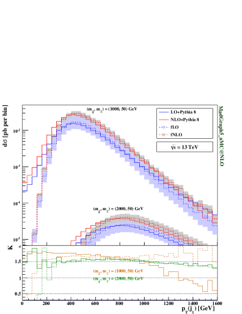
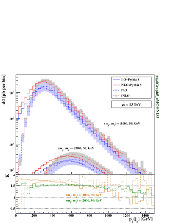
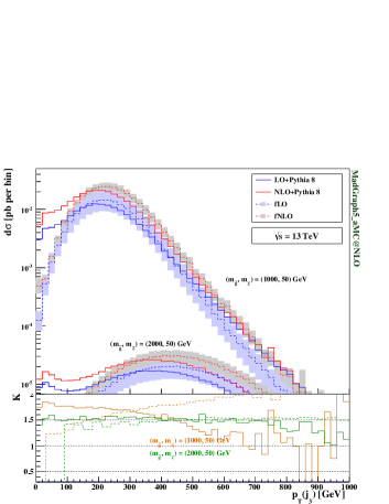
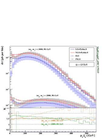
LHC phenomenology – In Table 1, we compute gluino pair-production total cross sections for proton-proton collisions at a center-of-mass energy of $\sqrt{s}=$13 TeV and for different gluino masses. Squarks are decoupled ($m_{\tilde{t}_{L}}=16$ TeV, $m_{\tilde{t}_{R}}=17$ TeV and $m_{\tilde{q}_{L}}=m_{\tilde{q}_{R}}=15$ TeV) so that any resonant squark contribution appearing in the real-emission topologies is off-shell and therefore suppressed. The latter production modes can be seen as the associated production of a gluino and a squark that subsequently decays into a gluino and a quark. Including these contributions as parts of the NLO QCD corrections for gluino pair-production would hence result in a double-counting when considering together all superpartner production processes inclusively. Moreover, these resonant channels require a special treatment in the fully-automated MadGraph5_aMC@NLO framework, that is left to future work Degrande et al. (pear). Our choice for the squark spectrum corresponds to the one made by ATLAS and CMS collaborations in their respective gluino searches Aad et al. (2014, ); Chatrchyan et al. (2014); Khachatryan et al. (2015).

Our results are evaluated both at the LO and NLO accuracy in QCD and presented together with scale and parton distribution (PDF) uncertainties. For the central values, we set the renormalization and factorization scales to half the sum of the transverse mass of all final state particles and use the NNPDF 3.0 set of parton distributions Ball et al. (2015) accessed via the LHAPDF 6 library Buckley et al. (2015). Scale uncertainties are derived by varying both scales independently by factors $\nicefrac{{1}}{{2}}$, $1$ and $2$, and the PDF uncertainties have been extracted from the cross section values spanned by all NNPDF distribution replicas following the NNPDF recommendations Demartin et al. (2010). We observe a significant enhancement of the cross section of about 50% due to genuine NLO contributions, as well as a sizable reduction of the uncertainties. In particular, the apparent drastic reduction of the PDF uncertainties is related to the poor quality of the LO NNPDF fit when compared to the NLO fit Ball et al. (2015).

In order to achieve realistic simulations of LHC collisions, we first handle gluino decays into two colored partons and a neutralino via an off-shell squark by using tree-level decay matrix-elements. For the fixed-order results presented below, we have analytically calculated those decay matrix elements and integrated them over the phase space, after checking our results with the MadSpin Artoisenet et al. (2013) and MadWidth Alwall et al. programs. These latter two programs have been used in the computation of the NLO predictions matched to parton showers. Due to the three-body nature of the gluino decays, spin correlations are here omitted as MadSpin can only handle them for two-body decays. We then interface the partonic events obtained in this way to a parton showering and hadronization description as provided by the Pythia 8 package Sjöstrand et al. (2015), and use the anti-$k_{T}$ jet reconstruction algorithm Cacciari et al. (2008) with a radius parameter set to 0.4, as implemented in FastJet Cacciari et al. (2012), to reconstruct all final state parton-level and hadron-level jets for fixed-order and parton-shower-matched calculations respectively. Finally, the phenomenological analysis of the generated events is performed with MadAnalysis 5 Conte et al. (2013).

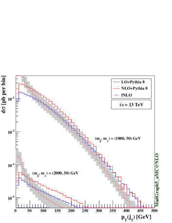
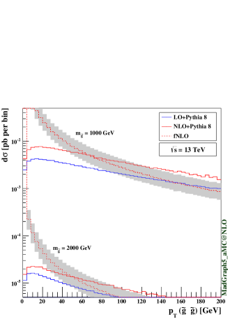
Key differential distributions particularly sensitive to both NLO and shower effects are presented in Fig. 1. We show the transverse-momentum ($p_{T}$) spectra of the first five leading jets (first five subfigures) for two benchmark scenarios featuring either a light ($m_{\tilde{g}}=1$ TeV) or a heavy ($m_{\tilde{g}}=2$ TeV) gluino, as well as a rather light bino ($m_{\chi}=50$ GeV). We compare fixed-order predictions (dashed) to results matched to parton showers (solid) and consider both LO (blue) and NLO (red) accuracy in QCD. We observe that most of the differential $K$-factors (i.e., the bin-by-bin ratios of the NLO result to the LO one) both with and without parton-shower matching strongly depend on the jet $p_{T}$ in the considered $p_{T}$ range. The NLO effects therefore not only increase the overall normalization of the distributions, but also distort their shapes. The $K$-factor is indeed greater at low $p_{T}$ than at high $p_{T}$, so that the traditional procedure of using LO predictions scaled by inclusive $K$-factors cannot be used for an accurate gluino signal description.

Fig. 1 also underlines the effects of matching LO and NLO matrix elements to parton showers. Since most parton-level jets originate from the decay of very massive gluinos, the fixed-order $p_{T}$ distributions peak at large $p_{T}$ values. In addition, the low-$p_{T}$ region of these spectra is depleted, with the exception of the fourth and fifth jet $p_{T}$ spectra where radiation effects are non-negligible. As a result of the matching to parton showers, the fixed-order NLO distributions are distorted and softened. While the change is milder in the large-$p_{T}$ tails whose shapes are controlled by the hard matrix element, the low-$p_{T}$ regions are mostly sensitive to effects due to multiple emissions and hence become populated. The parton shower emissions from hard partons are indeed often not reclustered back with the jet they are issued from, hence distorting the jet $p_{T}$ spectra. For this reason, resummation effects become significant below the peak of the various $p_{T}$ distributions. This effect is also illustrated on the last subfigure of Fig. 1, where we show the $p_{T}$ spectrum of the gluino pair in the small $p_{T}$ range. We have verified that the matched results agree with the fixed-order ones for very large $p_{T}$ values of the order of the gluino mass.

Conclusions – We have performed the first calculation of NLO supersymmetric QCD corrections to gluino pair-production matched to parton showers and have studied the impact of both the NLO contributions and of the parton showers. We have shown that observable effects could be induced on quantities typically used to obtain exclusion limits and that more accurate calculations are crucial for extracting model parameters in case of a discovery.

Our calculation has been performed fully automatically and we have applied it to the case of a simplified model similar to one of those used by the ATLAS and CMS collaborations for their respective gluino searches. In addition, we have publicly released the UFO model associated with our computation, that is sufficiently general to be readily used to explore the phenomenology associated with any supersymmetric QCD process.

Finally, our results also shows that all technical obstacles for automating the matching of fixed-order calculations for inclusive supersymmetric particle production at the NLO in QCD to parton showers have been cleared, up to the ambiguity issue of the double counting arising in real emission resonant contributions Degrande et al. (pear).