The variation of the fine-structure constant from disformal couplings

Abstract

We study a theory in which the electromagnetic field is disformally coupled to a scalar field, in addition to a usual non–minimal electromagnetic coupling. We show that disformal couplings modify the expression for the fine–structure constant, $\alpha$. As a result, the theory we consider can explain the non–zero reported variation in the evolution of $\alpha$ by purely considering disformal couplings. We also find that if matter and photons are coupled in the same way to the scalar field, disformal couplings itself do not lead to a variation of the fine–structure constant. A number of scenarios are discussed consistent with the current astrophysical, geochemical, laboratory and the cosmic microwave background radiation constraints on the cosmological evolution of $\alpha$. The models presented are also consistent with the current type Ia supernovae constraints on the effective dark energy equation of state. We find that the Oklo bound in particular puts strong constraints on the model parameters. From our numerical results, we find that the introduction of a non–minimal electromagnetic coupling enhances the cosmological variation in $\alpha$. Better constrained data is expected to be reported by ALMA and with the forthcoming generation of high–resolution ultra–stable spectrographs such as PEPSI, ESPRESSO, and ELT–HIRES. Furthermore, an expected increase in the sensitivity of molecular and nuclear clocks will put a more stringent constraint on the theory.

1 Introduction

The idea on the variation of the fundamental constants of physics was first raised by Dirac in his ‘large numbers hypothesis’ [1]. The advent of higher-dimensional theories [2, 3], in which the effective (3+1)-dimensional constants can vary in space and time, has led to an increased interest in nature’s fundamental constants and their variation. Despite this, Einstein’s equivalence principle, and hence local position invariance, is one of the building blocks of gravitational metric theories, which include amongst others the well-known gravitational theory of general relativity. Hence, the link between the constancy of fundamental constants and the equivalence principle is a natural one.

Recent observations have shown the possibility of the variation of one of these fundamental constants of nature, the electromagnetic fine-structure constant, $\alpha=e^{2}/4\pi\epsilon_{0}\hbar c\simeq 1/137$ [4]. Weaker constraints on the variation of the electromagnetic fine-structure constant have been derived from Big Bang Nucleosynthesis (BBN) at $z\sim 10^{9}$ [5] and the cosmic microwave background (CMB) radiation at $z\sim 10^{3}$ [6]. More stringent bounds have been reported at lower redshifts from astrophysical [7, 8, 9, 10, 11, 12, 13, 14, 15, 16, 17, 18], geochemical [19, 20, 21] and laboratory [22] constraints.

In this work, we will be considering a theoretical model containing three distinct metrics, related by a disformal transformation. We will specify our scalar-gravitational sector in what we will later call the Einstein Frame, in which the action looks like general relativity with an added scalar field. We then specify two other distinct frames in which we define matter and radiation separately. The latter two frames are described by two separate metrics, $\tilde{g}^{(i)}_{\mu\nu}$, although both of these metrics are disformally related with the scalar-gravitational metric, $g_{\mu\nu}$. Such disformal transformations have been introduced by Bekenstein [23], where in general a disformal transformation is characterized by the following relation

$$\tilde{g}^{(i)}_{\mu\nu}=C_{i}(\phi,X)g_{\mu\nu}+D_{i}(\phi,X)\phi_{,\mu}\phi_{,\nu}$$ (1.1)

where $X=(1/2)g^{\mu\nu}\phi_{,\mu}\phi_{,\nu}$ is the kinetic term. The first term is the widely known conformal coupling, whereas the second term is referred to as the disformal coupling. In what follows, we will be considering both couplings to depend on $\phi$ only. The line elements of these disformal metrics are now related by $d\tilde{s}_{i}^{2}=C_{i}ds^{2}+D_{i}(\phi_{,\mu}dx^{\mu})^{2}$, and as a result null four-vectors with respect to $g_{\mu\nu}$ could be either spacelike or timelike four-vectors with respect to the disformal metric $\tilde{g}^{(i)}_{\mu\nu}$. Furthermore, a conformal transformation can be viewed as an angle preserving metric rescaling mapping, although a disformal transformation deforms the spacetime to a preferred direction characterized by the gradient of the fields resulting in a distortion of both angles and lengths [24].

Disformal relations as described in (1.1) have been used in different scenarios, including inflation [25], varying speed of light theories [26, 27, 28], massive gravity [29, 30], dark energy [31, 32, 33, 34] and others. It was shown in [35] that disformal transformations preserve second order field equations and play, in the Horndeski theory, a similar role conformal transformations play in the scalar-tensor theories. See e.g. [36] on current constraints on universal disformal couplings.

The most immediate way to obtain a space and time variation of the electromagnetic fine-structure constant is to introduce a non–minimal coupling between the scalar field and electromagnetic fields [37, 38, 39, 40, 41]. It has been shown that such a non–minimal coupling give rise to nonconservation of the photon number along geodesics [42] which result in a modification of the distance-duality relation [37, 43, 44, 45, 46, 47, 48] and CMB spectrum distortion [37, 49, 50]. Similar results have also been reported in disformal scalar-tensor theories [51, 52]. We will show that such non–minimal coupling is not necessary to explain this non-zero variation of $\alpha$, as we can reproduce a varying electromagnetic fine-structure coupling purely by the introduced disformally related metrics.

We introduce our model in Section 2 and present the cosmological equations in Section 2.1 in which we give the relevant equations that we then use for our examples. In Section 3 we list the observational constraints that we use in order to choose our model parameters, which we then present and discuss in Section 4.

2 Disformal Electrodynamics: The Model

We consider the following action, consisting of a gravitational sector, a matter sector and an electromagnetic sector, respectively:

$${\cal S}={\cal S}_{\rm grav}\left(g_{\mu\nu},\phi\right)+S_{\rm matter}({\tilde{g}}_{\mu\nu}^{(m)})+S_{\rm EM}(A_{\mu},{\tilde{g}}_{\mu\nu}^{(r)}).$$ (2.1)

The metrics ${\tilde{g}}_{\mu\nu}^{(m)}$ and ${\tilde{g}}_{\mu\nu}^{(r)}$ are related to $g_{\mu\nu}$ via a disformal transformation:

$${\tilde{g}}_{\mu\nu}^{(m)} =C_{m}g_{\mu\nu}+D_{m}\phi_{,\mu}\phi_{,\nu}~{},$$ (2.2)

$${\tilde{g}}_{\mu\nu}^{(r)} =C_{r}g_{\mu\nu}+D_{r}\phi_{,\mu}\phi_{,\nu}~{}.$$ (2.3)

Here, $C_{r,m}$ and $D_{r,m}$ are functions of the scalar field. The functions $C_{r,m}$ are conformal factors, whereas the functions $D_{r,m}$ are disformal couplings. At this point, we do not specify the gravitational sector. Instead, we study the consequences of the disformally coupled scalar field on the propagation of electromagnetic waves. We aim to work in the Jordan Frame, by which we mean the frame in which matter is decoupled from the scalar degree of freedom. We therefore perform a disformal transformation of the action above such that all parts of the action are written in terms of the metric $\tilde{g}_{\mu\nu}^{(m)}$. The electromagnetic sector is specified by

$${\cal S}_{\rm EM}=-\frac{1}{4}\int d^{4}x\sqrt{-\tilde{g}^{(r)}}h(\phi)\tilde{g}_{(r)}^{\mu\nu}\tilde{g}_{(r)}^{\alpha\beta}F_{\mu\alpha}F_{\nu\beta}-\int d^{4}x\sqrt{-\tilde{g}^{(m)}}\tilde{g}_{(m)}^{\mu\nu}j_{\mu}A_{\mu},$$ (2.4)

where $F_{\mu\nu}$ is the standard antisymmetric Faraday tensor, $F_{\mu\nu}=\partial_{\mu}A_{\nu}-\partial_{\nu}A_{\mu}$, and $j^{\mu}$ is the four–current. The function $h(\phi)$ is the direct coupling between the electromagnetic field and the scalar. Note that $\tilde{g}^{(r)}_{\mu\nu}$ can also be written as

$$\tilde{g}^{(r)}_{\mu\nu}=\frac{C_{r}}{C_{m}}\tilde{g}_{\mu\nu}^{(m)}+\left(D_{r}-\frac{C_{r}D_{m}}{C_{m}}\right)\phi_{,\mu}\phi_{,\nu}\equiv A\tilde{g}^{(m)}_{\mu\nu}+B\phi_{,\mu}\phi_{,\nu},$$ (2.5)

Then, in terms of this metric the electromagnetic sector becomes

$$\begin{split}{\cal S}_{\rm EM}=&-\frac{1}{4}\int d^{4}x\sqrt{-\tilde{g}^{(m)}}h(\phi)Z\left[\tilde{g}^{\mu\nu}_{(m)}\tilde{g}^{\alpha\beta}_{(m)}-2\gamma^{2}\tilde{g}^{\mu\nu}_{(m)}\phi^{,\alpha}\phi^{,\beta}\right]F_{\mu\alpha}F_{\nu\beta}~{}\\ &-\int d^{4}x\sqrt{-\tilde{g}^{(m)}}{\tilde{g}}_{(m)}^{\mu\nu}j_{\mu}A_{\mu}~{},\end{split}$$ (2.6)

where we raise the indices with the metric $\tilde{g}^{(m)}_{\mu\nu}$ and define

$$Z=\left(1+\frac{B}{A}\tilde{g}^{\mu\nu}_{(m)}\partial_{\mu}\phi\partial_{\nu}\phi\right)^{1/2},$$ (2.7)

together with

$$\gamma^{2}=\frac{B}{A+B\tilde{g}^{\mu\nu}_{(m)}\partial_{\mu}\phi\partial_{\nu}\phi}~{}.$$ (2.8)

Note that the term proportional to $\gamma^{4}$ vanishes due to the antisymmetry of $F_{\mu\nu}$. Furthermore, note that gauge invariance implies $\tilde{\nabla}_{\mu}j^{\mu}=0$, where the covariant derivative is compatible with the metric $\tilde{g}_{\mu\nu}^{(m)}$. The field equations can be readily obtained by varying the action with respect to $A_{\mu}$, which results in

$$\tilde{\nabla}_{\epsilon}\left(h(\phi)ZF^{\epsilon\rho}\right)-\tilde{\nabla}_{\epsilon}\left(h(\phi)Z\gamma^{2}\phi^{,\beta}\left(\tilde{g}_{(m)}^{\epsilon\nu}\phi^{,\rho}-\tilde{g}_{(m)}^{\rho\nu}\phi^{,\epsilon}\right)F_{\nu\beta}\right)=j^{\rho}~{}.$$ (2.9)

where we again raise the indices with $\tilde{g}_{\mu\nu}^{(m)}$. The first term in the action (2.6) contains two parts: the first part consists of the kinetic term for the vector potential $A_{\mu}$; the second part is an interaction term between the disformally coupled scalar field and $A_{\mu}$. The latter vanishes in the case of vanishing disformal couplings. From the form of the action (2.6) we might naively think that the fine-structure coupling is simply given by $\alpha\propto 1/hZ$. This is not the case, as we shall show. To identify the effective electromagnetic coupling (or the ”fine–structure constant”) $\alpha$, we start by deriving the field equation for the electric field in Minkowski space $\left(\tilde{g}_{\mu\nu}^{(m)}=\eta_{\mu\nu}\right)$ and set the bare speed of light $c=1$. We also consider the scalar field to be a function of time only. From the obtained field equation (2.9), and using the fact that the electric field is identified by, $E^{i}=F^{i0}$, we find that the field equation for the electric field is given by

$$\nabla\cdot{\bf E}=\frac{Z\rho}{h(\phi)}$$ (2.10)

where $\rho=j^{0}$ is the charge density. By integrating this equation over a volume ${\cal V}$, it is straightforward to derive the electrostatic potential $V$ (for which ${\bf E}=-\nabla V$), which is found to be $V(r)=ZQ/(4\pi h(\phi)r)$, where $Q$ is the total charge contained in ${\cal V}$. Comparing this to the standard expression for the tree-level-potential from QED, one finds that $\alpha$ has the following dependence on $Z$ and $h$:

$$\alpha\propto\frac{Z}{h(\phi)}.$$ (2.11)

Note that if matter and radiation couple in the same way to the scalar field (i.e. ${\tilde{g}}_{\mu\nu}^{(m)}={\tilde{g}}_{\mu\nu}^{(r)}$ for which $A=1$ and $B=0$) we have $Z=1$ and we recover the usual form $\alpha\propto h(\phi)^{-1}$ [37, 53, 54, 55, 56, 57, 58, 59, 60].

2.1 Cosmology

We now specify our gravitational-scalar action to be as follows

$${\cal S}_{\rm grav}\left(g_{\mu\nu},\phi\right)=\int d^{4}x\sqrt{-g}\left(\frac{M_{\rm Pl}^{2}}{2}R-\frac{1}{2}g^{\mu\nu}\partial_{\mu}\phi\partial_{\nu}\phi-V(\phi)\right)$$ (2.12)

where $R$ is the Ricci scalar calculated with respect to the metric $g_{\mu\nu}$. From now on, reduced Planck units are assumed: $M_{\rm Pl}=1$. Hence, the theory we consider is given in the Einstein Frame as

$$\begin{split}{\cal S}=&\int d^{4}x\sqrt{-g}\left(\frac{1}{2}R-\frac{1}{2}g^{\mu\nu}\partial_{\mu}\phi\partial_{\nu}\phi-V(\phi)\right)+S_{\rm matter}({\tilde{g}}_{\mu\nu}^{(m)})\\ &-\frac{1}{4}\int d^{4}x\sqrt{-\tilde{g}^{(r)}}h(\phi)\tilde{g}_{(r)}^{\mu\nu}\tilde{g}_{(r)}^{\alpha\beta}F_{\mu\alpha}F_{\nu\beta}.\end{split}$$ (2.13)

The last term in the action above describes the dynamics of the CMB photons. From now on, we will refer to the three distinctive frames as the Einstein Frame (EF), Radiation Frame (RF) and Jordan Frame (JF) corresponding to the metrics $g_{\mu\nu},\;\tilde{g}_{\mu\nu}^{(r)}$ and $\tilde{g}_{\mu\nu}^{(m)}$ respectively. We define the RF as the frame in which all electromagnetic quantities are defined in their standard way. Furthermore, we define the JF as the frame in which matter is uncoupled from the scalar field. Since the gravity-scalar part of the action is written in its simplest form in the EF, we will be working in this frame and not in the other two frames where in general this part of the action has a nonstandard form.

By the variation of the action (2.13) with respect to the metric $g_{\mu\nu}$, we obtain the Einstein Field Equations

$$G^{\mu\nu}=T^{\mu\nu}_{\phi}+T^{\mu\nu}_{(m)}+T^{\mu\nu}_{(r)},$$ (2.14)

with $G^{\mu\nu}=R^{\mu\nu}-\frac{1}{2}g^{\mu\nu}R$ being the usual Einstein tensor in the EF. The energy-momentum tensors of the scalar field, matter and radiation are denoted by $T^{\mu\nu}_{\phi},\;T^{\mu\nu}_{(m)}$ and $T^{\mu\nu}_{(r)}$ respectively. We specify these energy-momentum tensors to be as follows

$$T_{\mu\nu}^{\phi} =\partial_{\mu}\phi\partial_{\nu}\phi-g_{\mu\nu}\left(\frac{1}{2}g^{\rho\sigma}\partial_{\rho}\phi\partial_{\sigma}\phi+V(\phi)\right),$$ (2.15)

$$T^{(m)}_{\mu\nu} =-\frac{2}{\sqrt{-g}}\frac{\delta(\sqrt{-\tilde{g}^{(m)}}\tilde{\mathcal{L}}_{m})}{\delta g^{\mu\nu}},$$ (2.16)

$$T^{(r)}_{\mu\nu} =-\frac{2}{\sqrt{-g}}\frac{\delta(\sqrt{-\tilde{g}^{(r)}}\tilde{\mathcal{L}}_{EM})}{\delta g^{\mu\nu}},$$ (2.17)

where we define the electromagnetic Lagrangian by $\tilde{\mathcal{L}}_{EM}=-\frac{1}{4}h(\phi)\tilde{g}_{(r)}^{\mu\nu}\tilde{g}_{(r)}^{\alpha\beta}F_{\mu\alpha}F_{\nu\beta}$ and denote the matter Lagrangian by $\mathcal{\tilde{L}}_{m}$. We now use the variation of the action (2.13) with respect to the scalar field, which leads us to the Klein-Gordon equation

$$\square\phi-V^{\prime}=-Q_{m}-Q_{r},$$ (2.18)

where we have introduced a matter coupling strength, $Q_{m}$, and a radiation coupling strength, $Q_{r}$, as follows

$$Q_{m} =\frac{C_{m}^{\prime}}{2C_{m}}T_{(m)}+\frac{D_{m}^{\prime}}{2C_{m}}\phi_{,\mu}\phi_{,\nu}T^{\mu\nu}_{(m)}-\nabla_{\mu}\left[\frac{D_{m}}{C_{m}}\phi_{,\nu}T^{\mu\nu}_{(m)}\right],$$ (2.19)

$$Q_{r} =\frac{C_{r}^{\prime}}{2C_{r}}T_{(r)}+\frac{D_{r}^{\prime}}{2C_{r}}\phi_{,\mu}\phi_{,\nu}T^{\mu\nu}_{(r)}+\frac{h^{\prime}}{h}C_{r}^{2}\sqrt{1+\frac{D_{r}}{C_{r}}g^{\mu\nu}\phi_{,\mu}\phi_{,\nu}}\;\mathcal{\tilde{L}}_{EM}-\nabla_{\mu}\left[\frac{D_{r}}{C_{r}}\phi_{,\nu}T^{\mu\nu}_{(r)}\right],$$ (2.20)

where $T_{(r)}$ and $T_{(m)}$ are the trace of $T^{\mu\nu}_{(r)}$ and $T^{\mu\nu}_{(m)}$ respectively, and in (2.20) we have also used (A.4). As a result of the Bianchi identities, the total energy-momentum tensor in the EF is covariantly conserved with respect to the EF metric, leading to the following conservation relation

$$\nabla_{\mu}(T^{\mu\nu}_{\phi}+T^{\mu\nu}_{(m)}+T^{\mu\nu}_{(r)})=0.$$ (2.21)

Although this holds for the total energy-momentum tensor, the couplings under consideration do not allow each of the energy-momentum tensors to be individually conserved. Indeed, by using (2.15), (2.18) and (2.21), we find that the matter and radiation conservation equations now read as follows

$$\nabla_{\mu}T^{\mu}_{(m)\nu} =Q_{m}\phi_{,\nu},$$ (2.22)

$$\nabla_{\mu}T^{\mu}_{(r)\nu} =Q_{r}\phi_{,\nu}.$$ (2.23)

A similar derivation is described in [51, 61, 62, 63, 64]. We shall now consider perfect fluid energy-momentum tensors for radiation and matter in the EF

$$T^{\mu\nu}_{(r)} =(\rho_{r}+p_{r})u^{\mu}u^{\nu}+p_{r}g^{\mu\nu},$$ (2.24)

$$T^{\mu\nu}_{(m)} =(\rho_{m}+p_{m})u^{\mu}u^{\nu}+p_{m}g^{\mu\nu},$$ (2.25)

where $\rho_{r}$ and $p_{r}$ are the EF radiation energy density and pressure respectively, similarly, $\rho_{m}$ and $p_{m}$ are the EF matter energy density and pressure respectively, and $u^{\mu}$ is the 4-velocity in the EF. By projecting the matter and radiation conservation equations along the 4-velocity, we obtain the following modified conservation equations

$$u^{\mu}\nabla_{\mu}\rho_{r}+(\rho_{r}+p_{r})\nabla_{\mu}u^{\mu} =-Q_{r}u^{\mu}\phi_{,\mu},$$ (2.26)

$$u^{\mu}\nabla_{\mu}\rho_{m}+(\rho_{m}+p_{m})\nabla_{\mu}u^{\mu} =-Q_{m}u^{\mu}\phi_{,\mu}.$$ (2.27)

These modified conservation equations show that energy is transferred from the scalar field, depicted by the term projecting the field gradient along the 4-velocity. We also define a perfect fluid energy-momentum tensor for both radiation and matter in the RF and JF respectively

$$\tilde{T}^{\mu\nu}_{(r)} =(\tilde{\rho}_{r}+\tilde{p}_{r})\tilde{u}^{\mu}\tilde{u}^{\nu}+\tilde{p}_{r}\tilde{g}^{\mu\nu}_{(r)},$$ (2.28)

$$\tilde{T}^{\mu\nu}_{(m)} =(\tilde{\rho}_{m}+\tilde{p}_{m})\tilde{u}^{\mu}\tilde{u}^{\nu}+\tilde{p}_{m}\tilde{g}^{\mu\nu}_{(m)}.$$ (2.29)

From now on, we will be considering a time-dependent scalar field, and a zero curvature Friedmann-Robertson-Walker (FRW) EF metric, given by $ds^{2}=g_{\mu\nu}dx^{\mu}dx^{\nu}=-dt^{2}+a^{2}(t)\delta_{ij}dx^{i}dx^{j}$, where $a(t)$ is the expansion scale factor. Following [39], we introduce an electromagnetic parametrisation,

$$\eta\equiv\frac{\mathcal{\tilde{L}}_{EM}}{\tilde{\rho}_{r}},$$ (2.30)

where $\eta$ could be positive or negative and have a modulus between 0 and $\approx 1$. We should note that in [39] they associate the $\eta$ parameter with matter energy density and not with radiation energy density. Also, by setting $\eta=1$ in the introduced electromagnetic parametrisation, and considering the special case $C_{r}(\phi)=C_{m}(\phi)=1$ together with $D_{r}(\phi)=D_{m}(\phi)=0$, we recover all the relevant equations given in [37], in which a statistical microscopic approach was employed. Using (A.10) we obtain a relationship between the energy density in the RF and that in the EF as follows

$$\tilde{\rho}_{r}=\frac{\rho_{r}}{C_{r}^{2}}\sqrt{1+\frac{D_{r}}{C_{r}}\phi_{,\mu}\phi^{,\mu}}.$$ (2.31)

Hence, we can then write the radiation coupling, $Q_{r}$, in terms of this $\eta$-parametrisation as follows

$$Q_{r}=\frac{C_{r}^{\prime}}{2C_{r}}T_{(r)}+\frac{D_{r}^{\prime}}{2C_{r}}\phi_{,\mu}\phi_{,\nu}T^{\mu\nu}_{(r)}+\frac{h^{\prime}}{h}\left[1+\frac{D_{r}}{C_{r}}\phi_{,\mu}\phi^{,\mu}\right]\eta\rho_{r}-\nabla_{\mu}\left[\frac{D_{r}}{C_{r}}\phi_{,\nu}T^{\mu\nu}_{(r)}\right].$$ (2.32)

For FRW cosmology, we find that the Klein-Gordon equation, (2.18), together with the conservation equations, (2.22) and (2.23), reduce to the following

$$\ddot{\phi}+3H\dot{\phi}+V^{\prime} =Q_{m}+Q_{r},$$ (2.33)

$$\dot{\rho}_{m}+3H(\rho_{m}+p_{m}) =-Q_{m}\dot{\phi},$$ (2.34)

$$\dot{\rho}_{r}+3H(\rho_{r}+p_{r}) =-Q_{r}\dot{\phi},$$ (2.35)

where $H=\dot{a}/a$ is the Hubble parameter and dot represents an EF time derivative. By using (2.33), (2.34), and (2.35), we can rewrite (2.19) and (2.32) as follows

$$Q_{m} =\frac{A_{r}}{A_{r}A_{m}-D_{r}D_{m}\rho_{r}\rho_{m}}\left[B_{m}-\frac{D_{m}B_{r}}{A_{r}}\rho_{m}\right],$$ (2.36)

$$Q_{r} =\frac{A_{m}}{A_{r}A_{m}-D_{r}D_{m}\rho_{r}\rho_{m}}\left[B_{r}-\frac{D_{r}B_{m}}{A_{m}}\rho_{r}\right],$$ (2.37)

where

$$A_{r} =C_{r}+D_{r}(\rho_{r}-\dot{\phi}^{2}),$$ (2.38)

$$A_{m} =C_{m}+D_{m}(\rho_{m}-\dot{\phi}^{2}),$$ (2.39)

$$B_{r} =\frac{1}{2}C_{r}^{\prime}[3w_{r}-1]\rho_{r}-\frac{1}{2}D_{r}^{\prime}\dot{\phi}^{2}\rho_{r}+\frac{h^{\prime}}{h}[C_{r}-D_{r}\dot{\phi}^{2}]\eta\rho_{r}+D_{r}\rho_{r}\left[\frac{C_{r}^{\prime}}{C_{r}}\dot{\phi}^{2}+V^{\prime}+3H\dot{\phi}\left(1+w_{r}\right)\right],$$ (2.40)

$$B_{m} =\frac{1}{2}C_{m}^{\prime}[3w_{m}-1]\rho_{m}-\frac{1}{2}D_{m}^{\prime}\dot{\phi}^{2}\rho_{m}+D_{m}\rho_{m}\left[\frac{C_{m}^{\prime}}{C_{m}}\dot{\phi}^{2}+V^{\prime}+3H\dot{\phi}\left(1+w_{m}\right)\right].$$ (2.41)

Using (A.12), it follows that for pressureless matter, the equation of state parameter in both frames is still zero, although according to (A.12), the equation of state parameter for radiation in the EF is now modified to [51, 65]

$$w_{r}=\frac{1}{3}\left(1-\frac{D_{r}}{C_{r}}\dot{\phi}^{2}\right),$$ (2.42)

where we have used the fact that in the RF, $\tilde{w}_{r}=1/3$. We find that the exact solutions for (2.34) and (2.35) are the following

$$\rho_{m} \propto\frac{C_{m}^{2}}{Y_{m}}\left(aC_{m}^{\frac{1}{2}}\right)^{-3},$$ (2.43)

$$\rho_{r} \propto\frac{C_{r}^{2}}{h^{\eta}Y_{r}}\left(aC_{r}^{\frac{1}{2}}\right)^{-4},$$ (2.44)

where we define $Y_{m}^{2}=1-(D_{m}/C_{m})\dot{\phi}^{2}$, $Y_{r}^{2}=1-(D_{r}/C_{r})\dot{\phi}^{2}$ and assume constant $\eta$ in (2.44). As expected, we find that $\tilde{\rho}_{m}\propto\tilde{a}_{(m)}^{-3}$ where $\tilde{a}_{(m)}$ is the scale factor in the JF, and that $\tilde{\rho}_{r}\propto h^{-\eta}\tilde{a}_{(r)}^{-4}$ where $\tilde{a}_{(r)}$ is the RF scale factor.

We now give the Friedmann equations in the EF obtained from the Einstein Field Equations (2.14)

$$H^{2} =\frac{1}{3}\left(\rho_{m}+\rho_{r}+\rho_{\phi}\right),$$ (2.45)

$$\dot{H} =-\frac{1}{6}\left[3\left(\rho_{m}+\dot{\phi}^{2}\right)+\rho_{r}\left(4-\frac{D_{r}}{C_{r}}\dot{\phi}^{2}\right)\right],$$ (2.46)

where we have also used (2.42), and defined the energy-momentum tensor of the scalar field as that of a perfect fluid with $\rho_{\phi}=(1/2)\dot{\phi}^{2}+V(\phi)$ and $p_{\phi}=(1/2)\dot{\phi}^{2}-V(\phi)$.

We admit that the scalar field characterizing the disformal coupling is also responsible for the current acceleration of the Universe, i.e., it is the dark energy. In order to compare our model’s dark energy equation of state parameter to type Ia supernova data set [66], we need to derive an effective equation of state parameter, $w_{\text{eff}}$, following [67, 65]. Experimental constraints on dark energy assume a non-interacting dark sector. On assuming that dark energy is given by a non-interacting perfect fluid, described by its equation of state parameter, $w_{\text{eff}}$, we can write the energy conservation equation as follows

$$\dot{\rho}^{\text{eff}}_{\text{DE}}=-3H(1+w_{\text{eff}})\rho^{\text{eff}}_{\text{DE}}.$$ (2.47)

By our dark sector assumption, dark matter is also assumed to be non-interacting, hence we can write the following Friedmann equation

$$H^{2}=\frac{1}{3}\left(a^{-4}\rho_{0,r}+a^{-3}\rho_{0,m}+\rho_{\text{DE}}^{\text{eff}}\right).$$ (2.48)

By comparing (2.48) and (2.45), we get the energy density of the effective dark energy fluid

$$\rho^{\text{eff}}_{\text{DE}}=\rho_{m}+\rho_{r}+\rho_{\phi}-a^{-4}\rho_{0,r}-a^{-3}\rho_{0,m}.$$ (2.49)

By taking the EF time derivative of (2.49), substituting the Klein-Gordon equation, (2.33), the matter conservation equation, (2.34), the radiation conservation equation, (2.35), and comparing the final equation with (2.47), we get the effective equation of state parameter as follows

$$w_{\text{eff}}=\frac{p_{\phi}+\rho_{r}\left(w_{r}-\frac{1}{3}a^{-4}\frac{\rho_{0,r}}{\rho_{r}}\right)}{\rho_{\text{DE}}^{\text{eff}}},$$ (2.50)

where $w_{r}$ is the equation of state parameter for radiation in the EF given by (2.42). We should mention that in the absence of radiation, matter and electromagnetic couplings, $w_{\text{eff}}$ reduces to the usual equation of state parameter for a quintessence scalar field, $w_{\phi}=p_{\phi}/\rho_{\phi}$.

3 Observational Constraints

We will only consider a choice of parameters for our models such that we agree with the measured cosmological, astrophysical, geochemical and laboratory parameters. Since we now have identified the fine-structure coupling $\alpha\propto Z\;h(\phi)^{-1}$, we can also define the temporal variation of $\alpha$, denoted by $\dot{\alpha}/\alpha$, where dot refers to the temporal derivative. As we are interested in solving our equations in a spatially-flat, homogeneous and isotropic Friedmann gravitational metric, and also a time-dependent scalar field, we here give the temporal variation of $\alpha$ in the mentioned setting. In this scenario, the coupling function $Z$, defined in (2.7), reduces to

$$Z=\left(\frac{1-\frac{D_{r}}{C_{r}}\dot{\phi}^{2}}{1-\frac{D_{m}}{C_{m}}\dot{\phi}^{2}}\right)^{\frac{1}{2}}~{}.$$ (3.1)

Furthermore, by considering the electromagnetic coupling, $h$, together with all the conformal and disformal couplings to be a function of $\phi$ only, it follows that $Z(\phi,\dot{\phi})$. We then arrive to the equation for the temporal variation of the fine-structure coupling

$$\frac{\dot{\alpha}}{\alpha}=\frac{1}{Z}\left(\frac{\partial Z}{\partial\phi}\dot{\phi}+\frac{\partial Z}{\partial\dot{\phi}}\ddot{\phi}\right)-\frac{1}{h}\frac{dh}{d\phi}\dot{\phi}.$$ (3.2)

Also, the redshift evolution of the fine-structure coupling is specified by the quantity

$$\frac{\Delta\alpha}{\alpha}(z)\equiv\frac{\alpha(z)-\alpha(z=0)}{\alpha(z=0)}=\frac{h(\phi_{0})Z(z)}{h(\phi(z))Z_{0}}-1,$$ (3.3)

where $\phi_{0}$ is the field value today and $Z_{0}$ is the value of $Z$ evaluated today. We recover the usual forms of the temporal variation and evolution of the fine-structure coupling, in Refs. [37, 53, 54, 55, 56, 57, 58, 59, 60], in the absence of disformal couplings. In order to choose our parameters will use:

1. the Union2.1 SNe Ia data set [66] and the Planck collaboration results [68], such that the present time measurements of our Universe agree with our final time boundary conditions. These results are summarized in Table 1. Since we are using a spatially-flat FRW EF metric, it follows that $\Omega_{0,\phi}\approx 0.7$.

   Parameter	Estimated value	Ref.
   $w_{0,\phi}$	$-1.006\pm 0.045$	[68]
   $H_{0}$	$(67.8\pm 0.9)\;\text{km}\;\text{s}^{-1}\text{Mpc}^{-1}$	[68]
   $\Omega_{0,m}$	$0.308\pm 0.012$	[68]

   Table 1: Listed are, respectively, the cosmological parameter, its estimated value, and the original reference.

2. the currently, most stringent atomic clock (AC) constraint on the present temporal variation of $\alpha$ [22]

   $$\left.\frac{\dot{\alpha}}{\alpha}\right|_{0}=(-1.6\pm 2.3)\times 10^{-17}\;\text{yr}^{-1},$$ (3.4)

3. an Oklo natural reactor constraint, in which self-sustained natural fission reactions took place at $\sim$ 2 Gyr ago $(z\simeq 0.16)$ [20, 21]

   $$\frac{|\Delta\alpha|}{\alpha}<1.1\times 10^{-8},$$ (3.5)

4. the ${{}^{187}}\text{Re}$ meteorite constraint over the age of the solar system $\sim$ 4.6 Gyr $(z\simeq 0.43)$ [19]

   $$\frac{\Delta\alpha}{\alpha}=(-8\pm 8)\times 10^{-7},$$ (3.6)

5. astrophysical data, including the 11 recently measured data set which contains the results of the Ultraviolet and Visual Echelle Spectrograph (UVES) [12, 13]. We list these measurements in Table 2, and plot the corresponding data points for the redshift evolution of $\Delta\alpha/\alpha$ in the figures of Section 4. We also use the large data set from Keck telescope and ESO’s Very Large Telescope (VLT) surveys carried out by Webb et al [7]. By assuming that $\Delta\alpha/\alpha$ values are described by a simple weighted mean, it is found that [17] $(\Delta\alpha/\alpha)_{\text{w}}=(-0.57\pm 0.11)\times 10^{-5}$ for the Keck quasi-stellar object (QSO) observations; while for the VLT quasar spectra observations, it is found that [15] $(\Delta\alpha/\alpha)_{\text{w}}=(0.208\pm 0.124)\times 10^{-5}$. These results differ from one another at the $\sim 4.7\sigma$ level, suggesting a dipole-like variation in $\alpha$. The binned many-multiplet (MM) VLT+Keck combined sample is also used in our $\Delta\alpha/\alpha$ redshift evolution plots, in which statistical errors for certain points have been increased prior to binning as reported in King et al [15]. We also use the weighted mean of the 21 Si IV doublets, $(\Delta\alpha/\alpha)_{\text{w}}=(-0.5\pm 1.3)\times 10^{-5}$, reported in Murphy et al [18] using the alkali-doublet (AD) method, together with two other results; $\Delta\alpha/\alpha=(-0.10\pm 0.22)\times 10^{-5}$ at $z=0.25$ and $\Delta\alpha/\alpha=(-0.08\pm 0.27)\times 10^{-5}$ at $z=0.68$; in which HI 21 cm absorption lines were used [14]. Other consistent results can be found in [16], and a detailed review on the constraints on $\Delta\alpha/\alpha$ can be found in [60, 69].

   Object	$z$	$(\Delta\alpha/\alpha)\times 10^{6}$	Spectrograph	Ref.
   Three sources	1.08	$4.3\pm 3.4$	HIRES	[8]
   HS1549+1919	1.14	$-7.5\pm 5.5$	UVES/HIRES/HDS	[13]
   HE0515-4414	1.15	$-0.1\pm 1.8$	UVES	[9]
   HE0515-4414	1.15	$0.5\pm 2.4$	HARPS/UVES	[10]
   HS1549+1919	1.34	$-0.7\pm 6.6$	UVES/HIRES/HDS	[13]
   HE0001-2340	1.58	$-1.5\pm 2.6$	UVES	[11]
   HE1104-1805A	1.66	$-4.7\pm 5.3$	HIRES	[8]
   HE2217-2818	1.69	$1.3\pm 2.6$	UVES	[12]
   HS1946+7658	1.74	$-7.9\pm 6.2$	HIRES	[8]
   HS1549+1919	1.80	$-6.4\pm 7.2$	UVES/HIRES/HDS	[13]
   Q1101-264	1.84	$5.7\pm 2.7$	UVES	[9]

   Table 2: Listed are, respectively, the object along each line of sight, the redshift of the absorber, the measurements of $\Delta\alpha/\alpha$, the spectrograph, and the original reference. The first measurement is the weighted average from eight absorbers in the redshift range $0.73<z<1.53$ along the lines of sight of three quasars reported in [8].

6. and the cosmic microwave background (CMB) radiation constraint $(z\simeq 10^{3})$ reported in [6]

   $$\frac{\Delta\alpha}{\alpha}=(3.6\pm 3.7)\times 10^{-3}.$$ (3.7)

The models presented in Section 4 satisfy the above constraints, even though, there are combinations of parameters that lead to cases which do not respect the Oklo bound. For example, some models in Fig. 1 do not pass the Oklo bound.

4 Analysis

In general, we will consider these specific forms of couplings and scalar field potential:

$$C_{i}(\phi) =\beta_{i}e^{x_{i}\phi},$$ (4.1)

$$D_{i}(\phi) =M_{i}^{-4}e^{y_{i}\phi},$$ (4.2)

$$h(\phi) =1-\zeta(\phi-\phi_{0}),$$ (4.3)

$$V(\phi) =M_{V}^{4}e^{-\lambda\phi}.$$ (4.4)

The introduced mass scales, $M_{i}$ and $M_{V}$, are tuned in order to obtain the correct cosmological parameters as listed in Table 1 together with an agreement with the temporal variation of the fine-structure coupling (3.4). Typically we find that $M_{i}\sim M_{V}\sim$ meV. In our models, we will only consider disformally coupled radiation, and hence we set $C_{r}(\phi)=1$ for all the models under consideration. On the other hand, whenever we consider a scalar field dependent conformal matter coupling, we also tune the dimensionless parameter, $\beta_{m}$, together with the other mass scales in order to agree with the measured cosmological parameters and temporal variation of the fine-structure coupling stringent constraint. Following the symmetry breaking argument in [70] for a slowly evolving time dependent scalar field, we only consider a linear electromagnetic coupling function. We are constrained on the magnitude of the dimensionless electromagnetic coupling parameter, $\zeta$, from local tests of the equivalence principle [60]

$$|\zeta_{\text{local}}|<10^{-3}$$ (4.5)

Another constraint on $\zeta$ was obtained in [71] using the CMB and large-scale structure data in combination with direct measurements of the expansion of the Universe, and more recently, another tighter constraint was obtained in [72] using more recent data, in which it was found that $|\zeta|<5\times 10^{-6}$.

We will now consider several models with different parameters. From our numerical results, we found that a change in the magnitude of $|\eta|$ between $0$ and $1$ has negligible effect on the results, so we set $\eta=1$ in all the models. We summarize the different parameter values for each specific model in Table 3, where we have neglected the parameters, $y_{m}$ and $y_{r}$, from the table as these parameters are both set to zero for the models shown in Fig. 1-3, although we do discuss a model with exponential disformal couplings in Section 4.1.

Fig.	$M_{r}$	$M_{m}$	$\beta_{m}$	$x_{m}$	$|\zeta|$	$M_{V}$	$\lambda$	$\left.(\dot{\alpha}/\alpha)\right|_{0}\times 10^{17}$
1	$\sim$ meV	$\sim$ meV	1	0	$<5\times 10^{-6}$	2.69 meV	0.45	$-2.14\sim-1.62$
2	$\sim$ meV	15 meV	8	0.14	0	2.55 meV	0.45	$-2.41\sim 0.70$
3	$\sim$ meV	15 meV	8	0.14	$<5\times 10^{-6}$	2.55 meV	0.45	$-2.10\sim-1.24$

Table 3: Listed are, respectively, the figure reference, the parameter values for each specific model, and the range of $\left.(\dot{\alpha}/\alpha)\right|_{0}$ for the range of parameter values considered in each figure.

The data points shown in the evolution with redshift of $\Delta\alpha/\alpha$ in Fig. 1-3 were taken from Section 3, as described therein. The respective data sets of the data points are listed in the legend of each plot, where UVES+HIRES+HDS+HARPS refer to the tabulated data points in Table 2. The constraints on $w_{\text{eff}}$ used in the plots depicting the evolution with redshift of the theoretical $w_{\text{eff}},w_{\phi}$ in Fig. 1-3 were taken from [66], where the results were obtained assuming a flat Universe for the joint data set of SNe, BAO, CMB, and $H_{0}$, with (dark/orange) and without (light/yellow) SN systematics. The dotted and dot-dashed lines in these plots depict the central value of $w_{\text{eff}}$ constraints with and without SN systematics in each redshift bin respectively. Although we start integrating our equations from $z=10^{3}$, at which we set $\phi_{\text{ini}}=1.5\;\text{M}_{\text{Pl}}$ as our initial condition, we restrict our plots in Fig. 1-3 to the redshift range where observational data is mostly concentrated.

4.1 Disformal couplings

In our first model, we consider disformally coupled radiation and matter in the absence of matter and radiation conformal couplings and set $\zeta=0$ in order to get a purely disformal case, without the addition of an electromagnetic coupling. This purely disformal case is an interesting model to consider, since it still predicts a non-zero variation of the fine-structure coupling, without the need of an electromagnetic coupling. The redshift evolution of $\Delta\alpha/\alpha$ is shown in Fig. 1, in which we consider constant matter and radiation disformal couplings. We have also considered a purely disformal case with exponential disformal couplings, by setting $M_{m}=M_{r}=100$ meV, $y_{m}=23.5$ and $y_{r}=1$, together with $M_{V}=4.75$ meV and $\lambda=2$. The latter two parameters were changed from those presented in Table 3 in order to be in agreement with the current cosmological parameters, whereas the exponential disformal coupling parameters were chosen such that the calculated temporal variation of the fine-structure coupling lies within the bounds of the estimated value measured by AC. Since the redshift evolutions of $\Delta\alpha/\alpha$, $\Omega_{i}$’s, $w_{\text{eff}}$, and $w_{\phi}$, for constant disformal couplings and exponential disformal couplings are indistinguishable, we only show the constant disformal couplings case in Fig. 1.

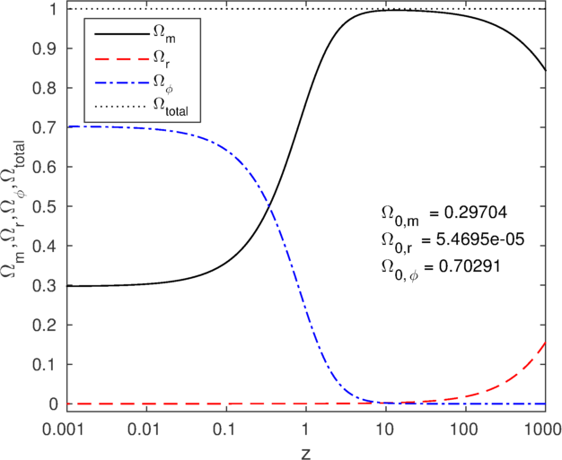
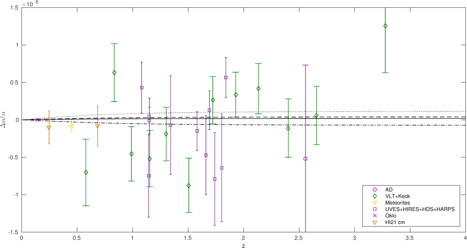
Figure 1: Redshift evolution of $\Omega_{i}$’s, $w_{\text{eff}}$, $w_{\phi}$ and $\Delta\alpha/\alpha$ when considering disformally coupled matter and radiation with and without an electromagnetic coupling. The solid line is the purely disformal case, whereas the dot-dashed, dashed, and dotted lines correspond to $\zeta=-4.9\times 10^{-6},\;1\times 10^{-6},\;4.9\times 10^{-6}$ respectively. The other model parameters are summarized in Table 3.

4.2 Conformal and disformal couplings

We now analyse the case in which we only consider matter to be conformally and disformally coupled together with disformally coupled radiation. An exponential matter conformal coupling together with constant disformal matter and radiation couplings are considered, as summarized in Table 3. The range of values for the constant disformal couplings are chosen such that the predicted current temporal variation in the fine-structure constant lies within the limits of the constraint given by (3.4), as these are the model parameters which directly affect the evolution of $\alpha$. We also restrict the values of the other model parameters, mainly the scalar field potential and the conformal matter coupling parameters in order to be in agreement with the current cosmological values listed in Table 1. Four different constant radiation energy scales are used in this model and shown in Fig. 2. We demonstrate that one can also get a non-zero value for the variation of $\alpha$, without the introduction of an electromagnetic coupling. This shows that we can still explain observational evidence for such a variation in the fine-structure coupling, without the need of an extra electromagnetic coupling. In these models $|\Delta\alpha/\alpha|$ at the CMB era is predicted to be $\mathcal{O}(10^{-8}-10^{-7})$ which is well within the current bounds.

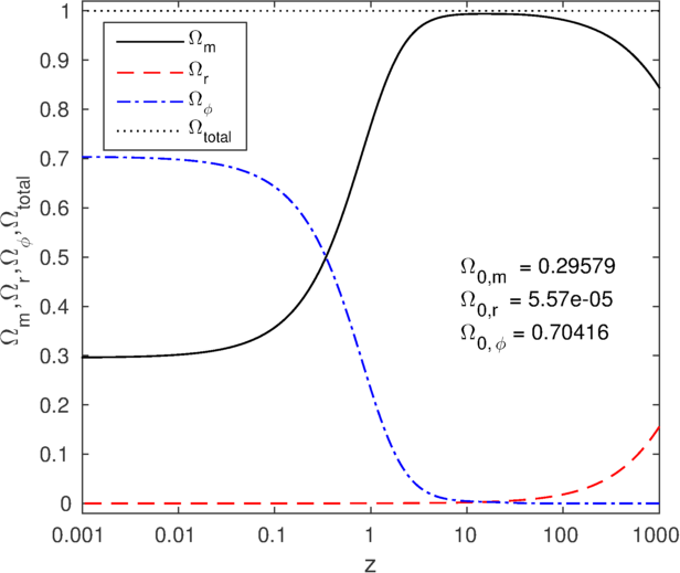
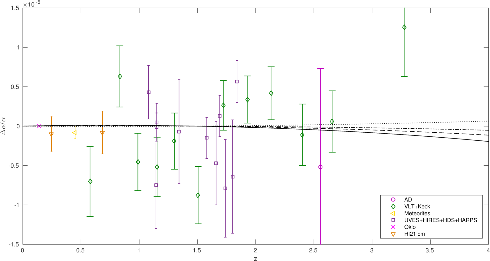
Figure 2: Redshift evolution of $\Omega_{i}$’s, $w_{\text{eff}}$, $w_{\phi}$ and $\Delta\alpha/\alpha$ when considering conformally and disformally coupled matter together with disformally coupled radiation in the absence of an electromagnetic coupling. The solid, dashed, dot-dashed, and dotted lines shown in the redshift evolution of $\Delta\alpha/\alpha$ plot correspond to $M_{r}=24.91,25.45,25.91,26.91$ meV respectively. The other parameters are summarized in Table 3.

4.3 Disformal and electromagnetic couplings

In this case, we consider matter and radiation to be disformally coupled together with an electromagnetic coupling. We again choose our model parameters so that we are in agreement with the data mentioned in Section  3. In Fig. 1 we only consider constant matter and radiation couplings, as described in Table 3. These disformal mass scales together with the non-zero $\zeta$ determine the evolution of the fine-structure coupling. We consider three different choices of these parameters, each giving a different redshift evolution of $\alpha$, although they all predict the same cosmology as long as the other independent parameters are left the same. The range of $|\Delta\alpha/\alpha|$ for these models at the CMB redshift is $\mathcal{O}(10^{-8}-10^{-6})$ which lies within the current CMB constraint. In Fig. 1 we also plot the purely disformal case, discussed in Section 4.1, in order to see the effect of the electromagnetic coupling on disformally coupled matter and radiation. We can clearly see that an electromagnetic coupling enhances the cosmological evolution of $\Delta\alpha/\alpha$.

4.4 Disformal, conformal and electromagnetic couplings

We now combine the previous cases together, where we are considering conformally and disformally coupled matter, and disformally coupled radiation, in the presence of an electromagnetic coupling. We choose a linear electromagnetic coupling as in (4.3) and an exponential conformal matter coupling. As in the previous cases, we choose our model parameters so that we are in agreement with the data mentioned in Section  3. In Fig. 3 we show different theoretical predictions of the variation of $\alpha$, when considering four different $\zeta$ and $M_{r}$ parameter choices as summarized in Table 3. In general, at least for our chosen parameters, we can conclude that the introduction of an electromagnetic coupling slightly enhances the variation of the fine-structure constant, still in agreement with current observational data. Indeed, for these models, $|\Delta\alpha/\alpha|$ at the CMB era is $\mathcal{O}(10^{-7}-10^{-6})$, still within the CMB constraint.

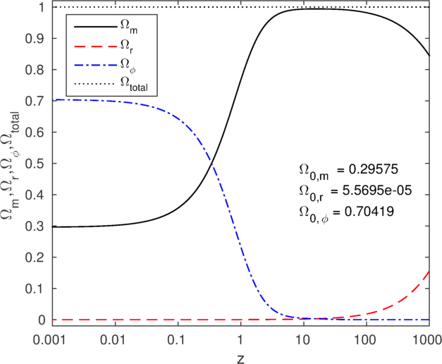
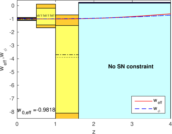
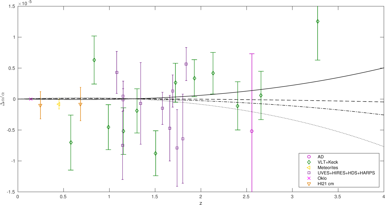
Figure 3: Redshift evolution of $\Omega_{i}$’s, $w_{\text{eff}}$, $w_{\phi}$ and $\Delta\alpha/\alpha$ when considering conformally and disformally coupled matter, and disformally coupled radiation in the presence of an electromagnetic coupling. The solid, dashed, dot-dashed and dotted lines correspond to $\zeta=-4.9\times 10^{-6},\;-1\times 10^{-6},\;1\times 10^{-6},\;4.9\times 10^{-6}$ respectively. The other model parameters are summarized in Table 3.

5 Conclusions

We have introduced the idea of disformally related metrics in order to explain the reported variations in the fine-structure constant. Our main conclusion is that we can naturally explain a non-zero variation in $\alpha$ by only considering disformally coupled radiation and matter. The introduction of an electromagnetic coupling has been exhaustively discussed in the literature and such models also predict a varying fine-structure constant. We have also considered the effect of this electromagnetic coupling in some of our models, and we can say that this coupling enhances the variational evolution of $\alpha$. We made sure that our chosen model parameters predict the current cosmological parameters in agreement with the experimental values together with an agreement with the reported bounds on variations in the fine-structure constant. From our numerical results, we found that when the present temporal variation of the fine-structure constant constraint is satisfied, the other geochemical and astrophysical constraints are also satisfied. We should still mention that the Oklo bound is not always satisfied by the chosen model parameters, although we do find some specific models which predict a variation in $\alpha$ that lies well within the Oklo constraint. We have also considered the weak constraint from the CMB, which is well satisfied in all our models.

High-resolution ultra-stable spectrographs are expected to increase the accuracy of the currently reported spectroscopic measurements. Such next generation spectrographs include PEPSI at the Large Binocular Telescope (LBT) in Arizona, ESPRESSO at the VLT [73], and ELT-HIRES at the European Extremely Large Telescope (E-ELT) [74, 75]. Consistency tests like the Sandage-Loeb cosmological redshift drift test could also be carried out in such facilities [76, 77, 78, 79]. The Atacama Large Millimeter/submillimeter Array (ALMA) [80, 81] is also expected to increase the sensitivity to detect radio continuum sources. Laboratory measurements with molecular and nuclear clocks are also expected to increase their sensitivity to as high as $10^{-21}\;\text{yr}^{-1}$ [82]. Other observational constraints coming from compact objects, such as white-dwarfs [83, 84], are equally being explored.

Appendix A: Disformal Transformations

We here derive some variable transformations between the EF and the tilde frames, the JF and RF. These mappings are also discussed in [51, 61, 62, 63, 64, 65], although we reproduce the relevant transformations for completeness. To keep the discussion simple, we write the JF metric (2.2) and RF metric (2.3) as a single tilde metric, which we write as

$$\tilde{g}_{\mu\nu}=Cg_{\mu\nu}+D\phi_{,\mu}\phi_{,\nu},$$ (A.1)

and then apply the variable transformations to each frame. From (A.1), it follows that the inverse metric is given by

$$\tilde{g}^{\mu\nu}=\frac{1}{C}\left(g^{\mu\nu}-\bar{\gamma}^{2}\partial^{\mu}\phi\partial^{\nu}\phi\right),$$ (A.2)

where

$$\bar{\gamma}^{2}=\frac{D}{C+Dg^{\mu\nu}\phi_{,\mu}\phi_{,\nu}}.$$ (A.3)

The determinants are related via

$$\sqrt{\frac{-\tilde{g}}{-g}}=C^{2}\sqrt{1+\frac{D}{C}\phi_{,\mu}\phi^{,\mu}}.$$ (A.4)

We now derive a relationship between the energy-momentum tensors in the EF metric and in the tilde metric (A.1). Using the definition of the energy-momentum tensor and the chain rule, we obtain the following

$$T^{\mu\nu}=\frac{2}{\sqrt{-g}}\frac{\delta(\sqrt{-\tilde{g}}\mathcal{\tilde{L}})}{\delta g_{\mu\nu}}=\sqrt{\frac{-\tilde{g}}{-g}}\frac{\delta\tilde{g}_{\alpha\beta}}{\delta g_{\mu\nu}}\left(\frac{2}{\sqrt{-\tilde{g}}}\frac{\delta(\sqrt{-\tilde{g}}\mathcal{\tilde{L}})}{\delta\tilde{g}_{\alpha\beta}}\right)=\sqrt{\frac{-\tilde{g}}{-g}}\frac{\delta\tilde{g}_{\alpha\beta}}{\delta g_{\mu\nu}}\tilde{T}^{\alpha\beta}.$$ (A.5)

Hence, together with (A.1)–(A.4), the contravariant and mixed energy-momentum tensor relations between the EF metric and tilde metric are as follows

$$T^{\mu\nu} =C^{3}\sqrt{1+\frac{D}{C}\phi_{,\mu}\phi^{,\mu}}\tilde{T}^{\mu\nu},$$ (A.6)

$$T^{\mu}_{\;\;\;\nu} =C^{2}\sqrt{1+\frac{D}{C}\phi_{,\mu}\phi^{,\mu}}\left[\delta^{\rho}_{\;\;\;\nu}-\frac{D\phi_{,\nu}\phi^{,\rho}}{C+D\phi_{,\mu}\phi^{,\mu}}\right]\tilde{T}^{\mu}_{\;\;\;\rho}.$$ (A.7)

On specifying a perfect fluid energy-momentum tensor in both frames,

$$T^{\mu\nu} =(\rho+p)u^{\mu}u^{\nu}+pg^{\mu\nu},$$ (A.8)

$$\tilde{T}^{\mu\nu} =(\tilde{\rho}+\tilde{p})\tilde{u}^{\mu}\tilde{u}^{\nu}+\tilde{p}\tilde{g}^{\mu\nu}.$$ (A.9)

we get the following mappings for the energy density, pressure and the equation of state parameter

$$\tilde{\rho} =\frac{\rho}{C^{2}}\sqrt{1+\frac{D}{C}\phi_{,\mu}\phi^{,\mu}},$$ (A.10)

$$\tilde{p} =\frac{p}{C^{2}\sqrt{1+\frac{D}{C}\phi_{,\mu}\phi^{,\mu}}},$$ (A.11)

$$\tilde{w}\equiv\frac{\tilde{p}}{\tilde{\rho}} =\frac{w}{1+\frac{D}{C}\phi_{,\mu}\phi^{,\mu}},$$ (A.12)

when considering a spatially-flat FRW EF metric and a time-dependent scalar field. Using this tilde metric (A.1), we also derive a relationship between the 4-velocity in the EF, $u^{\mu}$, and that in the tilde frame, $\tilde{u}^{\mu}$, given by the following equation

$$\tilde{u}^{\mu}=\frac{u^{\mu}}{\sqrt{C}\sqrt{1+\frac{D}{C}\phi_{,\mu}\phi^{,\mu}}}.$$ (A.13)

References

- [1] P. A. M. Dirac, The Cosmological constants, Nature 139 (1937) 323.
- [2] A. Chodos and S. L. Detweiler, Where Has the Fifth-Dimension Gone?, Phys. Rev. D21 (1980) 2167.
- [3] Y.-S. Wu and Z. Wang, The Time Variation of Newton’s Gravitational Constant in Superstring Theories, Phys. Rev. Lett. 57 (1986) 1978.
- [4] P. Mohr, B. Taylor, and D. Newell, The 2014 codata recommended values of the fundamental physical constants (web version 7.0), 2015. This database was developed by J. Baker, M. Douma, and S. Kotochigova. Available: http://physics.nist.gov/constants [Thursday, 27-Aug-2015 10:53:20 EDT]. National Institute of Standards and Technology, Gaithersburg, MD 20899.
- [5] F. Iocco, G. Mangano, G. Miele, O. Pisanti, and P. D. Serpico, Primordial Nucleosynthesis: from precision cosmology to fundamental physics, Phys. Rept. 472 (2009) 1–76, [arXiv:0809.0631].
- [6] Planck: Collaboration, P. A. R. Ade et al., Planck intermediate results - XXIV. Constraints on variations in fundamental constants, Astron. Astrophys. 580 (2015) A22, [arXiv:1406.7482].
- [7] J. K. Webb, J. A. King, M. T. Murphy, V. V. Flambaum, R. F. Carswell, and M. B. Bainbridge, Indications of a spatial variation of the fine structure constant, Phys. Rev. Lett. 107 (2011) 191101, [arXiv:1008.3907].
- [8] A. Songaila and L. L. Cowie, Constraining the Variation of the Fine Structure Constant with Observations of Narrow Quasar Absorption Lines, Astrophys. J. 793 (2014) 103, [arXiv:1406.3628].
- [9] P. Molaro, D. Reimers, I. I. Agafonova, and S. A. Levshakov, Bounds on the fine structure constant variability from FeII absorption lines in QSO spectra, Eur. Phys. J. ST 163 (2008) 173–189, [arXiv:0712.4380].
- [10] H. Chand, R. Srianand, P. Petitjean, B. Aracil, R. Quast, and D. Reimers, On the variation of the fine-structure constant: Very high resolution spectrum of QSO HE 0515-4414, Astron. Astrophys. 451 (2006) 45–56, [astro-ph/0601194].
- [11] I. I. Agafonova, P. Molaro, S. A. Levshakov, and J. L. Hou, First measurement of Mg isotope abundances at high redshifts and accurate estimate of , Astron. Astrophys. 529 (2011) A28, [arXiv:1102.2967].
- [12] P. Molaro et al., The UVES Large Program for Testing Fundamental Physics: I Bounds on a change in alpha towards quasar HE 2217-2818, Astron. Astrophys. 555 (2013) A68, [arXiv:1305.1884].
- [13] T. M. Evans et al., The UVES Large Program for testing fundamental physics – III. Constraints on the fine-structure constant from three telescopes, Mon. Not. Roy. Astron. Soc. 445 (2014), no. 1 128–150, [arXiv:1409.1923].
- [14] M. T. Murphy, J. K. Webb, V. V. Flambaum, M. J. Drinkwater, F. Combes, and T. Wiklind, Improved constraints on possible variation of physical constants from H I 21cm and molecular QSO absorption lines, Mon. Not. Roy. Astron. Soc. 327 (2001) 1244, [astro-ph/0101519].
- [15] J. A. King, J. K. Webb, M. T. Murphy, V. V. Flambaum, R. F. Carswell, M. B. Bainbridge, M. R. Wilczynska, and F. E. Koch, Spatial variation in the fine-structure constant – new results from VLT/UVES, Mon. Not. Roy. Astron. Soc. 422 (2012) 3370–3413, [arXiv:1202.4758].
- [16] H. Rahmani, R. Srianand, N. Gupta, P. Petitjean, P. Noterdaeme, and D. A. Vásquez, Constraining the variation of fundamental constants at z using 21-cm absorbers, Mon. Not. Roy. Astron. Soc. 425 (2012) 556–576, [arXiv:1206.2653].
- [17] M. T. Murphy, V. V. Flambaum, J. K. Webb, V. V. Dzuba, J. X. Prochaska, and A. M. Wolfe, Constraining variations in the fine - structure constant, quark masses and the strong interaction, Lect. Notes Phys. 648 (2004) 131–150, [astro-ph/0310318].
- [18] M. T. Murphy, J. K. Webb, V. V. Flambaum, J. X. Prochaska, and A. M. Wolfe, Further constraints on variation of the fine structure constant from alkali doublet QSO absorption lines, Mon. Not. Roy. Astron. Soc. 327 (2001) 1237, [astro-ph/0012421].
- [19] K. A. Olive, M. Pospelov, Y.-Z. Qian, G. Manhes, E. Vangioni-Flam, A. Coc, and M. Casse, A Re-examination of the Re-187 bound on the variation of fundamental couplings, Phys. Rev. D69 (2004) 027701, [astro-ph/0309252].
- [20] Y. Fujii, A. Iwamoto, T. Fukahori, T. Ohnuki, M. Nakagawa, H. Hidaka, Y. Oura, and P. Moller, Nuclear data in Oklo and time variability of fundamental coupling constants, in International Conference on Nuclear Data for Science and Technology (ND 2001): Embracing the Future at the Beginning of the 21st Century Tsukuba, Japan, October 7-12, 2001, 2002. hep-ph/0205206.
- [21] E. D. Davis and L. Hamdan, Reappraisal of the limit on the variation in implied by the Oklo natural fission reactors, Phys. Rev. C92 (2015), no. 1 014319, [arXiv:1503.06011].
- [22] T. Rosenband, D. Hume, P. Schmidt, C. Chou, A. Brusch, L. Lorini, W. Oskay, R. Drullinger, T. Fortier, J. Stalnaker, S. Diddams, W. Swann, N. Newbury, W. Itano, D. Wineland, and B. J., Frequency Ratio of and Single-Ion Optical Clocks; Metrology at the 17th Decimal Place, Science 319 (2008), no. 5871 1808.
- [23] J. D. Bekenstein, The Relation between physical and gravitational geometry, Phys. Rev. D48 (1993) 3641–3647, [gr-qc/9211017].
- [24] T. Koivisto, D. Wills, and I. Zavala, Dark D-brane Cosmology, JCAP 1406 (2014) 036, [arXiv:1312.2597].
- [25] N. Kaloper, Disformal inflation, Phys. Lett. B583 (2004) 1–13, [hep-ph/0312002].
- [26] M. A. Clayton and J. W. Moffat, Dynamical mechanism for varying light velocity as a solution to cosmological problems, Phys. Lett. B460 (1999) 263–270, [astro-ph/9812481].
- [27] J. Magueijo, New varying speed of light theories, Rept. Prog. Phys. 66 (2003) 2025, [astro-ph/0305457].
- [28] B. A. Bassett, S. Liberati, C. Molina-Paris, and M. Visser, Geometrodynamics of variable speed of light cosmologies, Phys. Rev. D62 (2000) 103518, [astro-ph/0001441].
- [29] C. de Rham and G. Gabadadze, Generalization of the Fierz-Pauli Action, Phys. Rev. D82 (2010) 044020, [arXiv:1007.0443].
- [30] C. de Rham, G. Gabadadze, and A. J. Tolley, Resummation of Massive Gravity, Phys. Rev. Lett. 106 (2011) 231101, [arXiv:1011.1232].
- [31] T. S. Koivisto, Disformal quintessence, arXiv:0811.1957.
- [32] M. Zumalacárregui, T. S. Koivisto, D. F. Mota, and P. Ruiz-Lapuente, Disformal Scalar Fields and the Dark Sector of the Universe, JCAP 1005 (2010) 038, [arXiv:1004.2684].
- [33] J. Sakstein, Towards Viable Cosmological Models of Disformal Theories of Gravity, Phys. Rev. D91 (2015), no. 2 024036, [arXiv:1409.7296].
- [34] J. Sakstein, Disformal Theories of Gravity: From the Solar System to Cosmology, JCAP 1412 (2014) 012, [arXiv:1409.1734].
- [35] D. Bettoni and S. Liberati, Disformal invariance of second order scalar-tensor theories: Framing the Horndeski action, Phys. Rev. D88 (2013) 084020, [arXiv:1306.6724].
- [36] P. Brax and C. Burrage, Constraining Disformally Coupled Scalar Fields, Phys. Rev. D90 (2014), no. 10 104009, [arXiv:1407.1861].
- [37] A. Hees, O. Minazzoli, and J. Larena, Breaking of the equivalence principle in the electromagnetic sector and its cosmological signatures, Phys. Rev. D90 (2014) 124064, [arXiv:1406.6187].
- [38] J. D. Bekenstein, Fine Structure Constant: Is It Really a Constant?, Phys. Rev. D25 (1982) 1527–1539.
- [39] H. B. Sandvik, J. D. Barrow, and J. Magueijo, A simple cosmology with a varying fine structure constant, Phys. Rev. Lett. 88 (2002) 031302, [astro-ph/0107512].
- [40] J. D. Barrow and S. Z. W. Lip, A Generalized Theory of Varying Alpha, Phys. Rev. D85 (2012) 023514, [arXiv:1110.3120].
- [41] J. D. Barrow and A. A. H. Graham, General Dynamics of Varying-Alpha Universes, Phys. Rev. D88 (2013) 103513, [arXiv:1307.6816].
- [42] O. Minazzoli, Conservation laws in theories with universal gravity/matter coupling, Phys. Rev. D88 (2013) 027506, [arXiv:1307.1590].
- [43] O. Minazzoli and A. Hees, Late-time cosmology of a scalar-tensor theory with a universal multiplicative coupling between the scalar field and the matter Lagrangian, Phys. Rev. D90 (2014), no. 2 023017, [arXiv:1404.4266].
- [44] I. Etherington, On the definition of distance in general relativity, Philos. Mag. 15 (1933), no. 7 761.
- [45] I. Etherington, Republication of: LX. On the definition of distance in general relativity, Gen. Relativ. Gravit. 39 (2007), no. 7 1055.
- [46] G. Ellis, On the definition of distance in general relativity: I. M. H. Etherington (Philosophical Magazine ser. 7, vol. 15, 761 (1933)), Gen. Relativ. Gravit. 39 (2007), no. 7 1047.
- [47] G. F. R. Ellis, Relativistic cosmology, Gen. Rel. Grav. 41 (2009) 581–660. [Proc. Int. Sch. Phys. Fermi47,104(1971)].
- [48] G. F. R. Ellis, R. Poltis, J.-P. Uzan, and A. Weltman, Blackness of the cosmic microwave background spectrum as a probe of the distance-duality relation, Phys. Rev. D87 (2013), no. 10 103530, [arXiv:1301.1312].
- [49] J. A. S. Lima, Thermodynamics of decaying vacuum cosmologies, Phys. Rev. D54 (1996) 2571–2577, [gr-qc/9605055].
- [50] J. A. S. Lima, A. I. Silva, and S. M. Viegas, Is the radiation temperature redshift relation of the standard cosmology in accordance with the data?, Mon. Not. Roy. Astron. Soc. 312 (2000) 747–752.
- [51] C. van de Bruck, J. Morrice, and S. Vu, Constraints on Nonconformal Couplings from the Properties of the Cosmic Microwave Background Radiation, Phys. Rev. Lett. 111 (2013) 161302, [arXiv:1303.1773].
- [52] P. Brax, C. Burrage, A.-C. Davis, and G. Gubitosi, Cosmological Tests of the Disformal Coupling to Radiation, JCAP 1311 (2013) 001, [arXiv:1306.4168].
- [53] T. Damour, F. Piazza, and G. Veneziano, Violations of the equivalence principle in a dilaton runaway scenario, Phys. Rev. D66 (2002) 046007, [hep-th/0205111].
- [54] T. Damour, F. Piazza, and G. Veneziano, Runaway dilaton and equivalence principle violations, Phys. Rev. Lett. 89 (2002) 081601, [gr-qc/0204094].
- [55] T. Damour and A. M. Polyakov, The String dilaton and a least coupling principle, Nucl. Phys. B423 (1994) 532–558, [hep-th/9401069].
- [56] T. Damour and A. M. Polyakov, String theory and gravity, Gen. Rel. Grav. 26 (1994) 1171–1176, [gr-qc/9411069].
- [57] E. J. Copeland, N. J. Nunes, and M. Pospelov, Models of quintessence coupled to the electromagnetic field and the cosmological evolution of alpha, Phys. Rev. D69 (2004) 023501, [hep-ph/0307299].
- [58] K. A. Olive and M. Pospelov, Evolution of the fine structure constant driven by dark matter and the cosmological constant, Phys. Rev. D65 (2002) 085044, [hep-ph/0110377].
- [59] N. J. Nunes and J. E. Lidsey, Reconstructing the dark energy equation of state with varying alpha, Phys. Rev. D69 (2004) 123511, [astro-ph/0310882].
- [60] J.-P. Uzan, Varying Constants, Gravitation and Cosmology, Living Rev. Rel. 14 (2011) 2, [arXiv:1009.5514].
- [61] M. Zumalacárregui and J. García-Bellido, Transforming gravity: from derivative couplings to matter to second-order scalar-tensor theories beyond the Horndeski Lagrangian, Phys. Rev. D89 (2014) 064046, [arXiv:1308.4685].
- [62] M. Zumalacárregui, T. S. Koivisto, and D. F. Mota, DBI Galileons in the Einstein Frame: Local Gravity and Cosmology, Phys. Rev. D87 (2013) 083010, [arXiv:1210.8016].
- [63] M. Minamitsuji, Disformal transformation of cosmological perturbations, Phys. Lett. B737 (2014) 139–150, [arXiv:1409.1566].
- [64] T. S. Koivisto, D. F. Mota, and M. Zumalacárregui, Screening Modifications of Gravity through Disformally Coupled Fields, Phys. Rev. Lett. 109 (2012) 241102, [arXiv:1205.3167].
- [65] C. van de Bruck and J. Morrice, Disformal couplings and the dark sector of the universe, JCAP 1504 (2015), no. 04 036, [arXiv:1501.03073].
- [66] N. Suzuki et al., The Hubble Space Telescope Cluster Supernova Survey: V. Improving the Dark Energy Constraints Above and Building an Early-Type-Hosted Supernova Sample, Astrophys. J. 746 (2012) 85, [arXiv:1105.3470].
- [67] S. Das, P. S. Corasaniti, and J. Khoury, Super-acceleration as signature of dark sector interaction, Phys. Rev. D73 (2006) 083509, [astro-ph/0510628].
- [68] Planck Collaboration, P. A. R. Ade et al., Planck 2015 results. XIII. Cosmological parameters, arXiv:1502.01589.
- [69] T. Chiba, The Constancy of the Constants of Nature: Updates, Prog. Theor. Phys. 126 (2011) 993–1019, [arXiv:1111.0092].
- [70] G. R. Dvali and M. Zaldarriaga, Changing with time: Implications for fifth force type experiments and quintessence, Phys. Rev. Lett. 88 (2002) 091303, [hep-ph/0108217].
- [71] E. Calabrese, E. Menegoni, C. J. A. P. Martins, A. Melchiorri, and G. Rocha, Constraining Variations in the Fine Structure Constant in the presence of Early Dark Energy, Phys. Rev. D84 (2011) 023518, [arXiv:1104.0760].
- [72] C. J. A. P. Martins and A. M. M. Pinho, Fine-structure constant constraints on dark energy, Phys. Rev. D91 (2015), no. 10 103501, [arXiv:1505.02196].
- [73] F. Pepe et al., ESPRESSO — An Echelle SPectrograph for Rocky Exo-planets Search and Stable Spectroscopic Observations, The Messenger (ESO) 153 (2013) 6.
- [74] ESO, “The e-elt construction proposal.” http://www.eso.org/public/products/books/book_0046, 2011. Accessed: 25/09/2015.
- [75] R. Maiolino et al., A Community Science Case for E-ELT HIRES, arXiv:1310.3163.
- [76] A. Sandage, The Change of Redshift and Apparent Luminosity of Galaxies due to the Deceleration of Selected Expanding Universes., Astrophys. J. 136 (1962) 319.
- [77] A. Loeb, Direct Measurement of Cosmological Parameters from the Cosmic Deceleration of Extragalactic Objects, Astrophys. J. 499 (1998) L111–L114, [astro-ph/9802122].
- [78] J. Liske et al., Cosmic dynamics in the era of Extremely Large Telescopes, Mon. Not. Roy. Astron. Soc. 386 (2008) 1192–1218, [arXiv:0802.1532].
- [79] P. E. Vielzeuf and C. J. A. P. Martins, Probing dark energy beyond with CODEX, Phys. Rev. D85 (2012) 087301, [arXiv:1202.4364].
- [80] V. Fish et al., High-Angular-Resolution and High-Sensitivity Science Enabled by Beamformed ALMA, arXiv:1309.3519.
- [81] R. P. J. Tilanus et al., Future mmVLBI Research with ALMA: A European vision, arXiv:1406.4650.
- [82] C. J. A. P. Martins, Fundamental cosmology in the E-ELT era: The status and future role of tests of fundamental coupling stability, Gen. Rel. Grav. 47 (2015), no. 1 1843, [arXiv:1412.0108].
- [83] J. Bagdonaite, E. J. Salumbides, S. P. Preval, M. A. Barstow, J. D. Barrow, M. T. Murphy, and W. Ubachs, Limits on a Gravitational Field Dependence of the Proton-Electron Mass Ratio from H2 in White Dwarf Stars, Phys. Rev. Lett. 113 (2014), no. 12 123002, [arXiv:1409.1000].
- [84] J. C. Berengut, V. V. Flambaum, A. Ong, J. K. Webb, J. D. Barrow, M. A. Barstow, S. P. Preval, and J. B. Holberg, Limits on the dependence of the fine-structure constant on gravitational potential from white-dwarf spectra, Phys. Rev. Lett. 111 (2013), no. 1 010801, [arXiv:1305.1337].