Preconditioning rectangular spectral collocation

Abstract

Rectangular spectral collocation (RSC) methods have recently been proposed to solve linear and nonlinear differential equations with general boundary conditions and/or other constraints. The involved linear systems in RSC become extremely ill-conditioned as the number of collocation points increase. By introducing suitable Birkhoff-type interpolation problems, we present pseudospectral integration preconditioning matrices for the ill-conditioned linear systems in RSC. The condition numbers of the preconditioned linear systems are independent of the number of collocation points. Numerical examples are given.

mmsxxxxxxxx–x

1 Introduction

Rectangular spectral collocation methods [3] have recently been demonstrated to be a convenient means of solving the problems when the row replacement or ‘boundary bordering’ strategy of standard spectral collocation methods [4, 11, 1, 2, 9] becomes ambiguous. Specifically, an $m$th-order differential operator is discretized by a rectangular matrix directly, allowing $m$ constraints to be appended to form an invertible square system. However, the involved linear systems become extremely ill-conditioned as the number of collocation points increases. Typically, the condition number grows like $N^{2m}$. Efficient preconditioners are highly required when solving the linear systems by an iterative method.

Recently, Wang, Samson, and Zhao [12] proposed a well-conditioned collocation method to solve linear differential equations with various types of boundary conditions. By introducing a suitable Birkhoff interpolation problem [10], they constructed a pseudospectral integration preconditioning matrix, which is the exact inverse of the pseudospectral discretization matrix of the $m$th-order derivative operator together with $m$ boundary conditions. In this paper, we employ the similar idea to construct a pseudospectral integration matrix, which is the exact inverse of the discretization matrix arising in the rectangular spectral collocation method for $m$th-order derivative operator together with $m$ general linear constraints. The condition number of the resulting linear system is independent of the number of collocation points when the new pseudospectral integration matrix is used as a right preconditioner for an $m$th-order linear differential operator together with the same constraints.

The rest of the paper is organized as follows. In §2, we review several topics required in the following sections. In §3, we introduce the new pseudospectral integration matrix by a suitable Birkhoff-type interpolation problem. In §4, we present the preconditioning rectangular spectral collocation method. Numerical examples are reported in §5. We present brief concluding remarks in §6.

2 Preliminaries

2.1 Barycentric resampling matrix

Let $\{x_{j}\}_{j=0}^{N}$ be a set of distinct interpolation points satisfying

(2.1) $$-1\leq x_{0}<x_{1}<\cdots<x_{N-1}<x_{N}\leq 1.$$

The associated barycentric weights are defined by

(2.2) $$w_{j,N}=\prod_{n=0,n\neq j}^{N}(x_{j}-x_{n})^{-1},\qquad j=0,1,\ldots,N.$$

Let $\{y_{j}\}_{j=0}^{M}$ be another set of distinct interpolation points satisfying

(2.3) $$-1\leq y_{0}<y_{1}<\cdots<y_{M-1}<y_{M}\leq 1.$$

The barycentric resampling matrix [3], ${\bf P}^{{\bf x}\mapsto{\bf y}}\in{\mathbb{R}^{(M+1)\times(N+1)}}$, which interpolates between the points $\{x_{j}\}_{j=0}^{N}$ and $\{y_{j}\}_{j=0}^{M}$, is defined by

$${\bf P}^{{\bf x}\mapsto{\bf y}}=[p^{{\bf x}\mapsto{\bf y}}_{ij}]_{i=0,j=0}^{M,N},$$

where

$$p^{{\bf x}\mapsto{\bf y}}_{ij}=\left\{\begin{array}[]{ll}\displaystyle\frac{w_{j,N}}{y_{i}-x_{j}}\left(\sum_{l=0}^{N}\displaystyle\frac{w_{l,N}}{y_{i}-x_{l}}\right)^{-1},&y_{i}\neq x_{j},\\ 1,&y_{i}=x_{j}.\end{array}\right.$$

Lemma 1.

If $N\geq M$, then ${\bf P}^{{\bf x}\mapsto{\bf y}}{\bf P}^{{\bf y}\mapsto{\bf x}}={\bf I}_{M+1}.$

2.2 Pseudospectral differentiation matrices

The Lagrange interpolation basis polynomials of degree $N$ associated with the points $\{x_{j}\}_{j=0}^{N}$ are defined by

$$\ell_{j,N}(x)=w_{j,N}\prod_{n=0,n\neq j}^{N}(x-x_{n}),\qquad j=0,1,\ldots,N,$$

where $w_{j,N}$ is the barycentric weight (2.2). Define the pseudospectral differentiation matrices:

$${\bf D}^{(m)}_{{\bf x}\mapsto{\bf x}}=\left[\ell_{j,N}^{(m)}(x_{i})\right]_{i,j=0}^{N},\qquad{\bf D}^{(m)}_{{\bf x}\mapsto{\bf y}}=\left[\ell_{j,N}^{(m)}(y_{i})\right]_{i=0,j=0}^{M,N}.$$

There hold

$${\bf D}^{(m)}_{{\bf x}\mapsto{\bf x}}=\left({\bf D}^{(1)}_{{\bf x}\mapsto{\bf x}}\right)^{m},\qquad m\geq 1,$$

and

$${\bf D}^{(m)}_{{\bf x}\mapsto{\bf y}}={\bf P}^{{\bf x}\mapsto{\bf y}}{\bf D}^{(m)}_{{\bf x}\mapsto{\bf x}}.$$

The matrix ${\bf D}^{(m)}_{{\bf x}\mapsto{\bf y}}$ is called a rectangular $m$th-order differentiation matrix, which maps values of a polynomial defined on $\{x_{j}\}_{j=0}^{N}$ to the values of its $m$th-order derivative on $\{y_{j}\}_{j=0}^{M}$. Explicit formulae and recurrences for rectangular differentiation matrices are given in [13].

2.3 Chebyshev polynomials and Chebyshev points

The most widely used spectral methods for non-periodic problems are those based on Chebyshev polynomials and Chebyshev points. In this paper, we focus on these polynomials and points. However, everything we discuss can be easily generalized to the case of Jacobi polynomials and corresponding points.

The Chebyshev points of the first kind (also known as Gauss-Chebyshev points) are given by

$$\nu_{j,N}=-\cos\frac{(2j+1)\pi}{2N+2},\qquad j=0,1,\ldots,N.$$

In this case, the Gauss-Chebyshev quadrature weights are given by [5]

$$\omega_{j,N}^{\nu}=\frac{\pi}{N+1},\qquad j=0,1,\ldots,N,$$

and the barycentric weights are given by [6]

$$w_{j,N}^{\nu}=(-1)^{N-j}\frac{2^{N}}{N+1}\sin\frac{(2j+1)\pi}{2N+2},\qquad j=0,1,\ldots,N.$$

Let $\mathbb{P}_{n}$ be the set of all algebraic polynomials of degree at most $n$. We have

(2.4) $$\int_{-1}^{1}\frac{p(x)}{\sqrt{1-x^{2}}}{\rm d}x=\sum_{j=0}^{N}\omega_{j,N}^{\nu}p(\nu_{j,N}),\qquad\forall p(x)\in\mathbb{P}_{2N+1}.$$

The Chebyshev points of the second kind (also known as Gauss-Chebyshev-Lobatto points) are given by

$$\tau_{j,N}=-\cos\frac{j\pi}{N},\qquad j=0,1,\ldots,N.$$

In this case, the Gauss-Chebyshev-Lobatto quadrature weights are given by [5]

$$\omega_{j,N}^{\tau}=\frac{\pi}{\rho_{j}N},\qquad j=0,\ldots,N,$$

and the barycentric weights are given by [8]

$$w_{j,N}^{\tau}=(-1)^{N-j}\frac{2^{N-1}}{\rho_{j}N},\qquad j=0,1,\ldots,N,$$

where

$$\rho_{0}=\rho_{N}=2,\qquad\rho_{1}=\rho_{2}=\cdots=\rho_{N-1}=1.$$

We have

$$\int_{-1}^{1}\frac{p(x)}{\sqrt{1-x^{2}}}{\rm d}x=\sum_{j=0}^{N}\omega_{j,N}^{\tau}p(\tau_{j,N}),\qquad\forall p(x)\in\mathbb{P}_{2N-1}.$$

Let $T_{n}(x)$ be the Chebyshev polynomials (see, for example, [5]) given by

$$T_{n}(x)=\cos(n\arccos x),\qquad x\in[-1,1].$$

They are mutually orthogonal:

(2.5) $$\int_{-1}^{1}\frac{T_{k}(x)T_{j}(x)}{\sqrt{1-x^{2}}}{\rm d}x=\frac{\varrho_{k}\pi}{2}\delta_{kj},$$

where

$$\varrho_{k}=\left\{\begin{array}[]{ll}2,&k=0,\\ 1,&k\geq 1,\end{array}\right.\qquad\delta_{kj}=\left\{\begin{array}[]{ll}1,&k=j,\\ 0,&k\neq j.\end{array}\right.$$

Let $\{\ell_{j,M}(x)\}_{j=0}^{M}$ denote the Lagrange interpolation basis polynomials of degree $M$ associated with the points $\{y_{j}\}_{j=0}^{M}$. The polynomial $\ell_{j,M}(x)$ can be rewritten as

(2.6) $$\ell_{j,M}(x)=\sum_{k=0}^{M}\beta_{kj}T_{k}(x),\qquad j=0,1,\ldots,M.$$

If $\{y_{j}\}_{j=0}^{M}$ is a subset of $\{\nu_{j,N}\}_{j=0}^{N}$ or $\{\tau_{j,N}\}_{j=0}^{N}$, $\beta_{kj}$ can be obtained with ease. For example, suppose that $\{y_{j}\}_{j=0}^{M}$ is a proper subset of $\{\nu_{j,N}\}_{j=0}^{N}$. Let $\varpi(\cdot)$ denote the map such that $y_{j}=\nu_{\varpi(j),N}$. Let $\mathcal{I}$ denote the set such that if $i\in\mathcal{I}$ then $\nu_{i,N}\notin\{y_{j}\}_{j=0}^{M}$. By (2.4) and (2.5), we have, for $j=0,1,\ldots,M,$

$$\beta_{kj}=\frac{2}{\varrho_{k}\pi}\left(T_{k}(y_{j})\omega_{\varpi(j),N}^{\nu}+\sum_{i\in\mathcal{I}}T_{k}(\nu_{i,N})\omega_{i,N}^{\nu}\ell_{j,M}(\nu_{i,N})\right),\qquad k=0,1,\ldots,M.$$

Here $\ell_{j,M}(\nu_{i,N})$, $i\in\mathcal{I}$, can be obtained by solving the following linear system

$$T_{k}(y_{j})\omega_{\varpi(j),N}^{\nu}+\sum_{i\in\mathcal{I}}T_{k}(\nu_{i,N})\omega_{i,N}^{\nu}\ell_{j,M}(\nu_{i,N})=0,\qquad k=M+1,\ldots,N.$$

In particular, if $\{\ell_{j,N}^{\nu}(x)\}_{j=0}^{N}$ denote the Lagrange interpolation basis polynomials of degree $N$ associated with $\{\nu_{j,N}\}_{j=0}^{N}$, we have

$$\ell_{j,N}^{\nu}(x)=\sum_{k=0}^{N}\beta_{kj}^{\nu}T_{k}(x),\qquad j=0,1,\ldots,N,$$

where, for $j=0,1,\ldots,N,$

$$\beta_{0j}^{\nu}=\frac{1}{N+1},$$

$$\beta_{kj}^{\nu}=\frac{2T_{k}(\nu_{j,N})}{N+1},\qquad k=1,2,\ldots,N-1,$$

$$\beta_{Nj}^{\nu}=(-1)^{N-j}\frac{2}{N+1}\sin\frac{(2j+1)\pi}{2N+2}.$$

If $\{\ell_{j,N}^{\tau}(x)\}_{j=0}^{N}$ denote the Lagrange interpolation basis polynomials of degree $N$ associated with $\{\tau_{j,N}\}_{j=0}^{N}$, we have

$$\ell_{j,N}^{\tau}(x)=\sum_{k=0}^{N}\beta_{kj}^{\tau}T_{k}(x),\qquad j=0,1,\ldots,N,$$

where, for $j=0,1,\ldots,N,$

$$\beta_{0j}^{\tau}=\frac{1}{\rho_{j}N},$$

$$\beta_{kj}^{\tau}=\frac{2T_{k}(\tau_{j,N})}{\rho_{j}N},\qquad k=1,2,\ldots,N-1,$$

$$\beta_{Nj}^{\tau}=\frac{(-1)^{N-j}}{\rho_{j}N}.$$

Define the integral operators:

$$\partial_{x}^{-1}v(x)=\int_{-1}^{x}v(t){\rm d}t;\qquad\partial_{x}^{-k}v(x)=\partial_{x}^{-1}\left(\partial_{x}^{-(k-1)}v(x)\right),\quad k\geq 2.$$

By

$$T_{n}(x)=\frac{T_{n+1}^{\prime}(x)}{2(n+1)}-\frac{T_{n-1}^{\prime}(x)}{2(n-1)},\qquad n\geq 2,$$

and

$$T_{n}(\pm 1)=(\pm 1)^{n},\qquad T_{n}^{\prime}(\pm 1)=\pm(\pm 1)^{n}n^{2},$$

we have

$$\partial_{x}^{-1}T_{0}(x)=1+x,$$

(2.7) $$\partial_{x}^{-1}T_{1}(x)=\frac{x^{2}-1}{2},$$

$$\partial_{x}^{-1}T_{n}(x)=\frac{T_{n+1}(x)}{2(n+1)}-\frac{T_{n-1}(x)}{2(n-1)}-\frac{(-1)^{n}}{n^{2}-1},\quad n\geq 2.$$

and

$$\partial_{x}^{-2}T_{0}(x)=\frac{(x+1)^{2}}{2},$$

$$\partial_{x}^{-2}T_{1}(x)=\frac{(x-2)(x+1)^{2}}{6},$$

(2.8) $$\partial_{x}^{-2}T_{2}(x)=\frac{x(x-2)(x+1)^{2}}{6}$$

$$\partial_{x}^{-2}T_{n}(x)=\frac{T_{n+2}(x)}{4(n+1)(n+2)}-\frac{T_{n}(x)}{2(n^{2}-1)}+\frac{T_{n-2}(x)}{4(n-1)(n-2)}$$

$$\hskip 56.9055pt-\frac{(-1)^{n}(1+x)}{n^{2}-1}-\frac{3(-1)^{n}}{(n^{2}-1)(n^{2}-4)},\quad n\geq 3.$$

3 Pseudospectral integration matrices

Given $\{y_{j}\}_{j=0}^{M}$ and $\{c_{j}\}_{j=0}^{M+m}$ with $m\geq 1$, we consider the Birkhoff-type interpolation problem:

$${\rm Find}\ p(x)\in\mathbb{P}_{M+m}\ {\rm such\ that}\ \left\{\begin{array}[]{ll}p^{(m)}(y_{j})=c_{j},&j=0,\ldots,M,\\ \mathcal{L}_{i}\left(p,\ldots,p^{(m-1)}\right)=c_{M+i},&i=1,\ldots,m,\end{array}\right.$$

where each $\mathcal{L}_{i}$ is a linear functional. Let $\{\ell_{j,M}(x)\}_{j=0}^{M}$ be the Lagrange interpolation basis polynomials of degree $M$ associated with the points $\{y_{j}\}_{j=0}^{M}$. Then the Birkhoff-type interpolation polynomial takes the form

(3.1) $$p(x)=\sum_{j=0}^{M}c_{j}\partial_{x}^{-m}\ell_{j,M}(x)+\sum_{i=0}^{m-1}{\alpha_{i}}x^{i},$$

where $\alpha_{i}$ can be determined by the linear constraints $\mathcal{L}_{i}(p,\ldots,p^{(m-1)})=c_{M+i}.$ Obviously, the existence and uniqueness of the Birkhoff-type interpolation polynomial is equivalent to that of $\{\alpha_{i}\}_{i=0}^{m-1}$. After obtaining $\alpha_{i}$, we can rewrite (3.1) as

$$p(x)=\sum_{j=0}^{M+m}c_{j}B_{j}(x),\qquad B_{j}(x)\in\mathbb{P}_{M+m}.$$

Let $N=M+m$ and $\{x_{i}\}_{i=0}^{N}$ be the points as in (2.1). Define the $m$th-order pseudospectral integration matrix (PSIM) as:

$${\bf B}^{(-m)}_{{\bf y}\mapsto{\bf x}}=\left[B_{j}(x_{i})\right]_{i,j=0}^{N}.$$

Define the matrices

$${\bf B}^{(k-m)}_{{\bf y}\mapsto{\bf x}}=\left[B_{j}^{(k)}(x_{i})\right]_{i,j=0}^{N},\qquad k\geq 1.$$

It is easy to show that

(3.2) $${\bf B}^{(k-m)}_{{\bf y}\mapsto{\bf x}}={\bf D}^{(k)}_{{\bf x}\mapsto{\bf x}}{\bf B}^{(-m)}_{{\bf y}\mapsto{\bf x}},\qquad k\geq 1.$$

Let ${\bf L}_{m}$ be the discretization of the linear constraints $\mathcal{L}_{i}$, $1\leq i\leq m$. We have the following theorem.

Theorem 2.

If for any $p(x)\in\mathbb{P}_{N}$,

$$\left[\begin{array}[]{c}\mathcal{L}_{1}\left(p,\ldots,p^{(m-1)}\right)\\ \vdots\\ \mathcal{L}_{m}\left(p,\ldots,p^{(m-1)}\right)\end{array}\right]={\bf L}_{m}\left[\begin{array}[]{c}p(x_{0})\\ \vdots\\ p(x_{N})\end{array}\right],$$

then

$$\left[\begin{array}[]{c}{\bf D}^{(m)}_{{\bf x}\mapsto{\bf y}}\\ {\bf L}_{m}\end{array}\right]{\bf B}^{(-m)}_{{\bf y}\mapsto{\bf x}}={\bf I}_{N+1}.$$

Proof.

The result follows from

$${\bf D}^{(m)}_{{\bf x}\mapsto{\bf x}}{\bf B}^{(-m)}_{{\bf y}\mapsto{\bf x}}=\left[\begin{array}[]{ll}{\bf P}^{{\bf y}\mapsto{\bf x}}&{\bm{0}}\end{array}\right],\qquad{\bf L}_{m}{\bf B}^{(-m)}_{{\bf y}\mapsto{\bf x}}=\left[\begin{array}[]{ll}{\bm{0}}&{\bf I}_{m}\end{array}\right],$$

and Lemma 1. ∎

Now we give concrete examples. Consider the non-separable linear constraint

(3.3) $$ap(-1)+bp(1)=\sigma,$$

and the global linear constraint

(3.4) $$\int_{-1}^{1}p(x){\rm d}x=\sigma,$$

where $a$, $b$ and $\sigma$ are given constants. They are straightforward to discretize: for (3.3),

$$\left[\begin{array}[]{lllll}a&0&\cdots&0&b\end{array}\right]{\bf p}=\sigma$$

and for (3.4),

$${\bf q}^{\rm T}{\bf p}={\bf\sigma},$$

where

$${\bf p}=\left[\begin{array}[]{cccc}p(x_{0})&p(x_{1})&\cdots&p(x_{N})\end{array}\right]^{\rm T}$$

and ${\bf q}$ is a column vector of Clenshaw-Curtis quadrature weights [5].

The first-order Birkhoff-type interpolation problem takes the form:

$${\rm Find}\ \ p(x)\in\mathbb{P}_{M+1}\ \ {\rm such\ that}\ \ \left\{\begin{array}[]{ll}p^{\prime}(y_{j})=c_{j},&j=0,1,\ldots,M,\\ \mathcal{L}p=c_{M+1}.&\end{array}\right.$$

• Given $\mathcal{L}p:=ap(-1)+bp(1)$ with $a+b\neq 0$, we have

  $$B_{j}(x)=\partial_{x}^{-1}\ell_{j,M}(x)-\frac{b}{a+b}\int_{-1}^{1}\ell_{j,M}(x){\rm d}x,\quad j=0,1,\ldots,M,$$

  $$B_{M+1}(x)=\frac{1}{a+b}.$$

• Given $\displaystyle\mathcal{L}p:=\int_{-1}^{1}p(x){\rm d}x$, we have

  $$B_{j}(x)=\partial_{x}^{-1}\ell_{j,M}(x)-\frac{1}{2}\int_{-1}^{1}\partial_{x}^{-1}\ell_{j,M}(x){\rm d}x,\quad j=0,1,\ldots,M,$$

  $$B_{M+1}(x)=\frac{1}{2}.$$

By (2.6) and (2.7), the matrix ${\bf B}^{(-1)}_{{\bf y}\mapsto{\bf x}}$ can be computed stably even for thousands of collocation points.

The second-order Birkhoff-type interpolation problem takes the form:

$${\rm Find}\ \ p(x)\in\mathbb{P}_{M+2}\ \ {\rm such\ that}\ \ \left\{\begin{array}[]{ll}p^{\prime\prime}(y_{j})=c_{j},&j=0,1,\ldots,M,\\ \mathcal{L}_{i}\left(p,p^{\prime}\right)=c_{M+i},&i=1,2.\end{array}\right.$$

• Given $\mathcal{L}_{1}(p,p^{\prime}):=ap(-1)+bp(1)$ with $a\neq b$, and $\mathcal{L}_{2}(p,p^{\prime})=\displaystyle\int_{-1}^{1}p(x){\rm d}x$, we have

  $$B_{j}(x)=\partial_{x}^{-2}\ell_{j,M}(x)-\frac{bx}{b-a}\int_{-1}^{1}\partial_{x}^{-1}\ell_{j,M}(x){\rm d}x$$

  $$\qquad\qquad+\left(\frac{(a+b)x}{2(b-a)}-\frac{1}{2}\right)\int_{-1}^{1}\partial_{x}^{-2}\ell_{j,M}(x){\rm d}x,\quad j=0,1,\ldots,M,$$

  $$B_{M+1}(x)=\frac{x}{b-a},$$

  $$B_{M+2}(x)=\frac{1}{2}-\frac{(a+b)x}{2(b-a)},$$

  and

  $$B_{j}^{\prime}(x)=\partial_{x}^{-1}\ell_{j,M}(x)-\frac{b}{b-a}\int_{-1}^{1}\partial_{x}^{-1}\ell_{j,M}(x){\rm d}x$$

  $$\qquad\qquad+\frac{a+b}{2(b-a)}\int_{-1}^{1}\partial_{x}^{-2}\ell_{j,M}(x){\rm d}x,\quad j=0,1,\ldots,M,$$

  $$B_{M+1}^{\prime}(x)=\frac{1}{b-a},$$

  $$B_{M+2}^{\prime}(x)=-\frac{a+b}{2(b-a)}.$$

By (2.6), (2.7) and (2.8), the matrices ${\bf B}^{(-2)}_{{\bf y}\mapsto{\bf x}}$ and ${\bf B}^{(1-2)}_{{\bf y}\mapsto{\bf x}}$ can be computed stably even for thousands of collocation points.

4 Preconditioning rectangular spectral collocation

Consider the $m$th-order differential equations of the form

(4.1) $$a_{m}(x)u^{(m)}(x)+\cdots+a_{1}(x)u^{\prime}(x)+a_{0}(x)u(x)=f(x),$$

together with linear constraints

(4.2) $$\mathcal{L}_{i}(u,\ldots,u^{(m-1)})=c_{M+i},\qquad i=1,2,\ldots,m.$$

Let $\{x_{j}\}_{j=0}^{N}$ (with $N=M+m$) and $\{y_{j}\}_{j=0}^{M}$ be the points as defined in (2.1) and (2.3), respectively. The rectangular spectral collocation discretization [3] of (4.1) is given by

$${\bf A}_{M+1}{\bf u}={\bf f},$$

where

$${\bf A}_{M+1}={\rm diag}\{{\bf a}_{m}\}{\bf D}^{(m)}_{{\bf x}\mapsto{\bf y}}+\cdots+{\rm diag}\{{\bf a}_{1}\}{\bf D}^{(1)}_{{\bf x}\mapsto{\bf y}}+{\rm diag}\{{\bf a}_{0}\}{\bf D}^{(0)}_{{\bf x}\mapsto{\bf y}}.$$

Here we use boldface letters to indicate a column vector obtained by discretizing at the points $\{y_{j}\}_{j=0}^{M}$ except for the unknown ${\bf u}$. For example,

$${\bf a}_{0}=\left[\begin{array}[]{cccc}a_{0}(y_{0})&a_{0}(y_{1})&\cdots&a_{0}(y_{M})\end{array}\right]^{\rm T},$$

$${\bf f}=\left[\begin{array}[]{cccc}f(y_{0})&f(y_{1})&\cdots&f(y_{M})\end{array}\right]^{\rm T}.$$

Let

$${\bf L}_{m}{\bf u}={\bf c}_{m}$$

be the discretization of the linear constraints (4.2) and satisfy the condition in Theorem 2, where

$${\bf c}_{m}=\left[\begin{array}[]{cccc}c_{M+1}&c_{M+2}&\cdots&c_{M+m}\end{array}\right]^{\rm T}.$$

The global collocation system is given by

(4.5) $${\bf Au=g}$$

where

$${\bf A}=\left[\begin{array}[]{c}{\bf A}_{M+1}\\ {\bf L}_{m}\end{array}\right],\quad{\bf g}=\left[\begin{array}[]{c}{\bf f}\\ {\bf c}_{m}\end{array}\right].$$

Consider the pseudospectral integration matrix ${\bf B}^{(-m)}_{{\bf y}\mapsto{\bf x}}$ (3) as a right preconditioner for the linear system (4.5). We need to solve the right preconditioned linear system

$${\bf A}{\bf B}^{(-m)}_{{\bf y}\mapsto{\bf x}}{\bf v}={\bf g}.$$

By (see Theorem 2)

$${\bf L}_{m}{\bf B}^{(-m)}_{{\bf y}\mapsto{\bf x}}=\left[\begin{array}[]{ll}{\bm{0}}&{\bf I}_{m}\end{array}\right],$$

we have

(4.7) $${\bf A}_{M+1}{\bf B}^{(-m)}_{{\bf y}\mapsto{\bf x}}\left[\begin{array}[]{c}{\bf I}_{M+1}\\ {\bm{0}}\end{array}\right]{\bf v}_{M+1}={\bf f}-{\bf A}_{M+1}{\bf B}^{(-m)}_{{\bf y}\mapsto{\bf x}}\left[\begin{array}[]{c}{\bm{0}}\\ {\bf I}_{m}\end{array}\right]{\bf c}_{m}.$$

There hold

$${\bf A}_{M+1}{\bf B}^{(-m)}_{{\bf y}\mapsto{\bf x}}\left[\begin{array}[]{c}{\bf I}_{M+1}\\ {\bm{0}}\end{array}\right]$$

$$= {\rm diag}\{{\bf a}_{m}\}+{\rm diag}\{{\bf a}_{m-1}\}\widetilde{\bf B}^{(m-1-m)}_{{\bf y}\mapsto{\bf y}}+\cdots+{\rm diag}\{{\bf a}_{0}\}\widetilde{\bf B}^{(0-m)}_{{\bf y}\mapsto{\bf y}},$$

and

$${\bf A}_{M+1}{\bf B}^{(-m)}_{{\bf y}\mapsto{\bf x}}\left[\begin{array}[]{c}{\bm{0}}\\ {\bf I}_{m}\end{array}\right]={\rm diag}\{{\bf a}_{m-1}\}\widehat{\bf B}^{(m-1-m)}_{{\bf y}\mapsto{\bf y}}+\cdots+{\rm diag}\{{\bf a}_{0}\}\widehat{\bf B}^{(0-m)}_{{\bf y}\mapsto{\bf y}},$$

where, for $k=0,1,\cdots,m-1$,

$$\widetilde{\bf B}^{(k-m)}_{{\bf y}\mapsto{\bf y}}=\left[B_{j}^{(k)}(y_{i})\right]_{i,j=0}^{M},\qquad\widehat{\bf B}^{(k-m)}_{{\bf y}\mapsto{\bf y}}=\left[B_{j}^{(k)}(y_{i})\right]_{i=0,j=M+1}^{M,M+m}.$$

After solving (4.7), we obtain ${\bf u}$ by

$${\bf u}={\bf B}^{(-m)}_{{\bf y}\mapsto{\bf x}}\left[\begin{array}[]{c}{\bf v}_{M+1}\\ {\bf c}_{m}\end{array}\right].$$

5 Numerical results

In this section, we compare the rectangular spectral collocation (RSC) scheme (4.5) and the preconditioned rectangular spectral collocation (P-RSC) scheme (4.7). In all computations, the Chebyshev points of the second kind are chosen as $\{x_{j}\}_{j=0}^{N}$ and the Chebyshev points of the first kind are chosen as $\{y_{j}\}_{j=0}^{M}$.

Example 1

We consider the equation

(5.1) $$u^{\prime}(x)+a_{0}(x)u(x)=f(x)$$

with the linear constraint

(5.2) $$u(-1)+u(1)=\sigma,$$

or the linear constraint

(5.3) $$\int_{-1}^{1}u(x){\rm d}x=\sigma,$$

where $\sigma$ is a given constant. We report in Table 1 the condition numbers of the linear systems in RSC and P-RSC with $a_{0}(x)=2x,-\sin x$, and various $N$. We observe that the condition numbers of P-RSC are independent of $N$, while those of RSC behave like $\mathcal{O}(N^{2.5})$.

Table 1: Comparison of condition numbers.

	$a_{0}(x)=2x$				$a_{0}(x)=-\sin x$
	Constraint (5.2)		Constraint (5.3)		Constraint (5.2)		Constraint (5.3)
$N$	RSC	P-RSC	RSC	P-RSC	RSC	P-RSC	RSC	P-RSC
128	6.86e+04	3.19	3.37e+04	2.54	3.04e+04	1.95	4.07e+04	1.95
256	3.87e+05	3.19	1.91e+05	2.54	1.72e+05	1.95	2.29e+05	1.95
512	2.19e+06	3.19	1.08e+06	2.54	9.68e+05	1.95	1.30e+06	1.95
1024	1.24e+07	3.19	6.10e+06	2.54	5.47e+06	1.95	7.32e+06	1.95

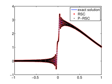
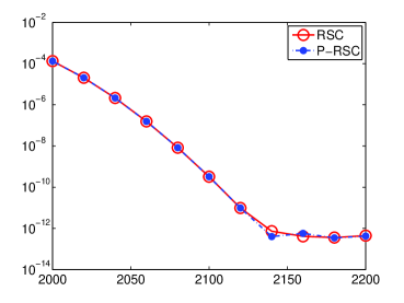
    (a)                                                                     (b)

Fig. 1: (a): exact solution versus numerical solutions. (b): comparison of numerical errors

We next consider (5.1) with $a_{0}(x)=2x$ and the linear constraint (5.2). The function $f(x)$ and $\sigma$ are chosen such that an oscillatory solution of (5.1) is

$$u(x)=100\exp(-x^{2})\int_{-1}^{x}\exp(t^{2})\sin(2000t^{2}){\rm d}t.$$

In Figure 1 (a) we plot the exact solution against the numerical solutions obtained by RSC and P-RSC with $N=2200$. In Figure 1 (b) we plot the maximum point-wise errors of RSC and P-RSC. It indicates that for this example, even for very large $N$, both RSC and P-RSC are very stable.

Example 2

We consider the equation

(5.4) $$\varepsilon u^{\prime\prime}(x)-xu^{\prime}(x)-u(x)=f(x)$$

with the linear constraints

$$u(-1)-u(1)=\sigma_{1},\qquad\int_{-1}^{1}u(x){\rm d}x=\sigma_{2}.$$

The function $f(x)$, $\sigma_{1}$ and $\sigma_{2}$ are chosen such that the exact solution of (5.4) is

$$u(x)=\exp\left(\frac{x^{2}-1}{2\varepsilon}\right).$$

Table 2: Comparison of condition numbers and iterations of different schemes for $\varepsilon=1$.

	RSC			P-RSC
$N$	Condition	Error	Iterations	Condition	Error	Iterations
128	1.95e+08	8.41e-10	$>$1000	2.73	6.66e-16	8
256	4.39e+09	9.23e-09	$>$1000	2.73	6.66e-16	8
512	9.94e+10	7.84e-08	$>$1000	2.73	8.88e-16	8
1024	2.25e+12	2.49e-06	$>$1000	2.73	1.11e-15	8

In Tables 2-4, we present the condition numbers, the maximum point-wise errors, and the number of iterations via the GMRES algorithm [7] with the relative tolerance equal to $10^{-10}$ and the restart number equal to $40$, for the cases $\varepsilon=1$, $\varepsilon=0.1$, and $\varepsilon=0.01$, respectively. We observe that the condition numbers of P-RSC are independent of $N$, while those of RSC behave like $\mathcal{O}(N^{4.5})$.

Table 3: Comparison of condition numbers and iterations of different schemes for $\varepsilon=0.1$.

	RSC			P-RSC
$N$	Condition	Error	Iterations	Condition	Error	Iterations
128	6.74e+07	2.65e-10	$>$1000	5.11e+02	1.14e-14	16
256	1.50e+09	5.95e-10	$>$1000	5.11e+02	1.62e-14	16
512	3.35e+10	4.12e-09	$>$1000	5.11e+02	1.58e-14	16
1024	7.55e+11	1.69e-07	$>$1000	5.11e+02	1.49e-14	16

Table 4: Comparison of condition numbers and iterations of different schemes for $\varepsilon=0.01$.

	RSC			P-RSC
$N$	Condition	Error	Iterations	Condition	Error	Iterations
128	4.47e+07	2.23e-10	$>$1000	3.70e+05	3.11e-13	64
256	9.77e+08	2.20e-09	$>$1000	3.70e+05	1.04e-12	65
512	2.16e+10	7.95e-09	$>$1000	3.70e+05	1.34e-12	67
1024	4.84e+11	4.69e-07	$>$1000	3.70e+05	5.35e-13	67

6 Concluding remarks

We have proposed a preconditioning rectangular spectral collocation scheme for $m$th-order ordinary differential equations together with $m$ general linear constraints. The condition number of the resulting linear system is typically independent of the number of collocation points. And the linear system can be solved by an iterative solver within a few iterations. The application of the preconditioning scheme to nonlinear problems is straightforward.

References

- [1] J. P. Boyd, Chebyshev and Fourier spectral methods, Dover Publications, Inc., Mineola, NY, second ed., 2001.
- [2] C. Canuto, M. Y. Hussaini, A. Quarteroni, and T. A. Zang, Spectral methods: Fundamentals in single domains, Scientific Computation, Springer-Verlag, Berlin, 2006.
- [3] T. A. Driscoll and N. Hale, Rectangular spectral collocation, IMA Journal of Numerical Analysis, to appear (2015).
- [4] B. Fornberg, A practical guide to pseudospectral methods, vol. 1 of Cambridge Monographs on Applied and Computational Mathematics, Cambridge University Press, Cambridge, 1996.
- [5] D. Funaro, Polynomial approximation of differential equations, vol. 8 of Lecture Notes in Physics. New Series m: Monographs, Springer-Verlag, Berlin, 1992.
- [6] P. Henrici, Essentials of numerical analysis with pocket calculator demonstrations, John Wiley & Sons, Inc., New York, 1982.
- [7] Y. Saad and M. H. Schultz, GMRES: a generalized minimal residual algorithm for solving nonsymmetric linear systems, SIAM J. Sci. Statist. Comput., 7 (1986), pp. 856–869.
- [8] H. E. Salzer, Lagrangian interpolation at the Chebyshev points , ; some unnoted advantages, Comput. J., 15 (1972), pp. 156–159.
- [9] J. Shen, T. Tang, and L.-L. Wang, Spectral methods, vol. 41 of Springer Series in Computational Mathematics, Springer, Heidelberg, 2011. Algorithms, analysis and applications.
- [10] Y. G. Shi, Theory of Birkhoff interpolation, Nova Science Publishers, Inc., Hauppauge, NY, 2003.
- [11] L. N. Trefethen, Spectral methods in MATLAB, vol. 10 of Software, Environments, and Tools, Society for Industrial and Applied Mathematics (SIAM), Philadelphia, PA, 2000.
- [12] L.-L. Wang, M. D. Samson, and X. Zhao, A well-conditioned collocation method using a pseudospectral integration matrix, SIAM J. Sci. Comput., 36 (2014), pp. A907–A929.
- [13] K. Xu and N. Hale, Explicit construction of rectangular differentiation matrices, IMA Journal of Numerical Analysis, to appear (2015).