A New Method for tackling Asymmetric Decision Problems

Abstract

Chain Event Graphs are probabilistic graphical models designed especially for the analysis of discrete statistical problems which do not admit a natural product space structure. We show here how they can be used for decision analysis, and describe an optimal decision strategy based on an efficient local computation message passing scheme. We briefly describe a method for producing a parsimonious decision CEG, analogous to the parsimonious ID, and touch upon the CEG-analogues of Shachter’s barren node deletion and arc reversal for ID-based solution.

Keywords: Chain Event Graph, decision analysis, Influence diagram

1 Introduction

In this paper we demonstrate how the Chain Event Graph (CEG) (see for example [14, 16, 15, 12, 1]) can be used for tackling asymmetric decision problems.

Extensive form (EF) decision trees (in which variables appear in the order in which they are observed by a decision maker) are flexible and expressive enough to represent asymmetries within both the decision and outcome spaces, doing this through the topological structure of the tree. They can however become unwieldy, and are not convenient representations from which to read the conditional independence structure of a problem.

Other graphical representations have been developed which to some extent deal with the complexity issue associated with decision trees, and also allow for local computation. The most commonly used of these is the Influence diagram (ID). Because of their popularity, ID solution techniques have developed considerably since their first introduction. However a major drawback of the ID representation is that many decision problems are asymmetric in that different actions can result in different choices in the future, and IDs are not ideally suited to this sort of problem [5]. As decision makers have become more ambitious in the complexity of the problems they wish to solve, standard ID and tree-based methods have proven to be inadequate, and new techniques have become necessary.

There have consequently been many attempts to adapt IDs for use with asymmetric problems (see for example  [13, 9, 8]), or to develop new techniques which use both IDs and trees [4]. There have also been several new structures suggested, such as Sequential Decision Diagrams (SDDs) [5] and Valuation Networks (VNs) [11]. Asymmetric problems have recently also been represented via decision circuits [2]. An overview of many of these developments is given by Bielza & Shenoy in [3]. They note that none of the methods available is consistently better than the others.

CEGs are probabilistic graphical models designed especially for the representation and analysis of discrete statistical problems which do not admit a natural product space structure. Unlike Bayesian Networks (BNs) they are functions of event trees, and this means that they are able to express the complete sample space structure associated with a problem. They are particularly useful for the analysis of processes where the future development at any specific point depends on the particular history of the problem up to that point. Such dependencies can be thought of as context-specific conditional independence properties; and the structure implied by these properties is fully expressed by the topology of the CEG. This is a distinct advantage over context-specific BNs, which require supplementary information usually in the form of trees or conditional probability tables attached to some of the vertices of the graph. Like BNs, CEGs provide a suitable framework for efficient local computation algorithms.

Using CEGs for asymmetric decision analysis overcomes drawbacks associated with the current graphs and techniques used for this purpose. They are an advance on decision trees as they encode the conditional independence structure of problems. They can represent probability models consistently (which SDDs don’t), and do not require dummy states or supplementing with extra tables or trees (a drawback of both VNs and Smith et als’ adaptations of IDs). They can model all asymmetries (which VNs cannot), and their semantics are very straightforward, making them an appropriate tool for use by non-experts (both VN & SDD methodologies are very complicated).

Call & Miller [4] have drawn attention to the value of coalescence in tree-based approaches to decision problems. They also point out that the difficulties in reading conditional independence structure from trees has meant that analysts using them have not fully taken advantage of the idea of coalescence. They remark that the ability to exploit asymmetry can be a substantial advantage for trees. If trees could naturally exploit coalescence, the efficiency advantage is even greater. SDDs go some way towards exploiting this [3], but decision CEGs use coalescence both as a key tool for the expression of conditional independence structure, and to power the analysis.

We show here how CEGs can be used for decision analysis, and describe how to arrive at an optimal decision strategy via an efficient local computation message passing scheme. We briefly describe a method for producing a parsimonious decision CEG, analogous to the parsimonious ID, which contains only those variables and dependencies which the decision maker needs to consider when making decisions; and touch upon the CEG-analogues of Shachter’s [10] barren node deletion and arc reversal for ID-based solution.

2 CEGs and decision CEGs

We start this section with a brief introduction to CEGs – we direct readers to one of [14, 15] if they would like a more detailed definition. The CEG is a function of a coloured event tree, so we begin with a description of these graphs.

• A coloured event tree $\cal{T}$ is a directed tree with a single root-node.

• Each non-leaf-node $v$ has an associated random variable whose state space corresponds to the subset of directed edges of $\cal{T}$ which emanate from $v$.

• Each edge leaving a node $v$ carries a label which identifies a possible immediate future development given the partial history corresponding to the node $v$.

• The non-leaf-node set of $\cal{T}$ is partitioned into equivalence classes called stages: Nodes in the same stage have sets of outgoing edges with the same labels, and edges with the same labels have the same probabilities.

• The edge-set of $\cal{T}$ is partitioned into equivalence classes, whose members have the same colour: Edges have the same colour when the vertices from which they emanate are in the same stage and the edges have the same label (& hence probability).

• The non-leaf-node set of $\cal{T}$ is also partitioned into equivalence classes called positions: Nodes are in the same position if the coloured subtrees rooted in these nodes are isomorphic both in topology and in colouring (so edges in one subtree are coloured (and labelled) identically with their corresponding edges in another).

Note that nodes are in the same position when the sets of complete future developments from each node are the same, and have the same probability distribution.

To produce a CEG $\cal{C}$ from our tree $\cal{T}$, nodes in the same position are combined (as in the coalesced tree), and all leaf-nodes are combined into a single sink-node. We note that for CEGs used for decision problems it is often more convenient to replace the single sink-node by a set of terminal utility nodes, each of which corresponds to a different utility value. We return to this idea in our example in Section 3.

So the nodes of our CEG $\cal{C}$ are the positions of the underlying tree $\cal{T}$. We transfer the ideas of stage and colour from $\cal{T}$ to $\cal{C}$, and it is this combination of positions and stages that enables the CEG to encode the full conditional independence structure of the problem being modelled [14].

Many discrete statistical processes are asymmetric in that some variables have quite different collections of possible outcomes given different developments of the process up to that point. It was for these sorts of problem that the CEG was created, and one area where they have proved particularly useful is that of causal analysis [16, 15]. In much causal analysis the question being asked is If I make this manipulation, what are the effects?, but graphical models set up to answer such questions can also be readily used for questions such as If I want to maximise my utility over this process, what are the manipulations (decisions) I need to make?

In attempting to answer this second question, we notice that there are only certain nodes or positions in the CEG which can actually be manipulated. We concentrate in this paper on manipulations which impose a probability of one onto one edge emanating from any such node (equivalent to making a firm decision). Hence the probabilistic nature of these nodes is removed – they become decision nodes, and we therefore draw them as squares.

We draw our CEG in EF order – as with decision trees this is necessary in order to calculate optimal decision rules. If two decision nodes in $\cal{T}$ are in the same position, then the optimal strategy is the same for the decision maker (DM) at each of the two decision nodes: it is conditionally independent of the path taken to reach the decision node. A similar interpretation can be given to two chance nodes in the same position.

The only other modification that is required to use the CEG for decision analysis is the addition of utilities. This can be done in two ways (1) adding utilities to edges, or (2) expanding the sink-node $w_{\infty}$ into a set of utility nodes, each corresponding to a distinct utility value (see our example in Section 3). We make our terminal nodes diamond-shaped whether they are leaf nodes or a single sink-node.

When we manipulate a CEG we prune edges that are given zero probability by the manipulation, and also any edge or position which lies downstream of such edges only. No other edges (except those we manipulate to) have probabilities changed by the manipulation [15]. This is not the case when we simply observe an event, when edge-probabilities upstream of the observation can also change.

In [7], Dawid outlines how a decision-theoretic approach can be taken to causal inference. In this paper we are perhaps doing the opposite; we show how established causal analysis techniques for CEGs have a natural application in the field of decision analysis.

Our propagation algorithm is illustrated in Table 1 – at the end of the local message passing, the root node will contain the maximum expected utility. In the pseudocode we use $C$ & $D$ for the sets of chance & decision nodes, $p$ represents a probability or weight, and $u$ a utility. The utility part of a position $w$ is denoted by $w[u]$, the probability part of an edge by $e(w,w^{\prime})[p]$ etc. The set of child nodes of a position $w$ is denoted by $ch(w)$. Note that there may be more than one edge connecting two positions, if say two different decisions have the same consequence. This has significant ramifications for more complicated problems, as described in our example.

Table 1: Local propagation algorithm for finding an optimal decision sequence

• Find a topological ordering of the positions. Without loss of generality call this $w_{1},w_{2},\ldots,w_{n}$, so that $w_{1}$ is the root-node, and $w_{n}$ is the sink-node.

• Initialize the utility value $w_{n}[u]$ of the sink node to zero.

• Iterate: for $i=n-1$ step minus 1 until $i=1$ do:

  • If $w_{i}\in C$ then $w_{i}[u]=\sum_{w\in ch(w_{i})}\big{[}\sum_{e(w_{i},w)}\big{[}e(w_{i},w)[p]*(w[u]+e(w_{i},w)[u])\big{]}\big{]}$

  • If $w_{i}\in D$ then $w_{i}[u]=\max_{w\in ch(w_{i})}\big{[}\max_{e(w_{i},w)}\big{[}(w[u]+e(w_{i},w)[u])\big{]}\big{]}$

• Mark the sub-optimal edges.

Note that when we choose to confine utilities to terminal utility nodes, this algorithm is much simplified since both the initializing step and the $e(w_{i},w)[u]$ components are no longer required.

3 Representing and solving asymmetric decision problems using extensive form CEGs

We concentrate here on how the CEG compares with the augmented ID of Smith, Holtzman & Matheson [13] for the representation and solution of asymmetric decision problems. We show that the ID-based solution techniques of barren-node deletion [10] and parsimony have direct analogues in the CEG-analysis, and that arc-reversal [10] is not required for the solution of EF CEGs. The distribution trees [13] added to the nodes of IDs to describe the asymmetry of a problem can simply be thought of as close-ups of interesting parts of the CEG-depiction, where they are an integral part of the representation rather than bolt-on as is the case with IDs. We illustrate this comparison through an example.

We first consider what is meant by conditional independence statements which involve decision variables.

The statement $X\amalg Y\ |\ Z$ is true if and only if we can write $P(x\ |\ y,z)$ as $a(x,z)$ for some function $a$ of $x$ and $z$, for all values $x,y,z$ of the variables $X,Y,Z$ [6]. So clearly, for chance variables $X,Y,Z$ and decision variable $D$, where the value taken by $X$ is not known to the DM when she makes a decision at $D$, we can write statements such as $X\amalg D\ |\ Z$ and $X\amalg Y\ |\ D$ since the expressions $P(x\ |\ d,z)=a(x,z)$ and $P(x\ |\ y,d)=a(x,d)$ are unambiguous in this situation ($d$ representing a value taken by $D$).

Note that $P(d\ |\ y,z)$ is not unambiguously defined, and so conditional independence is no longer a symmetric property when we add decision variables to the mix. By a slight abuse of notation we can also write $U\amalg(Y,D_{1})\ |\ (Z,D_{2})$ if $U(y,z,d_{1},d_{2})=U(z,d_{2})$ for all values $y,z,d_{1},d_{2}$ of the chance variables $Y,Z$ and decision variables $D_{1},D_{2}$.

Example. Patients suffering from some disease are given one of a set of possible treatments. There is an initial reaction to the treatment in that the patient’s body either accepts the treatment without problems or attempts to reject it. After this initial reaction, the patient responds to the treatment at some level measurable by their doctor, and this response is independent of the initial reaction conditioned on which treatment has been given. The patient’s doctor has to make a second decision on how to continue treatment.

There is also the possibility of the patient having some additional condition which affects how they will respond to the treatment. Whether or not they have this condition will remain unknown to the doctor, but she can estimate the probability of a patient having it or not (conditioned on their response to their particular treatment) from previous studies.

The doctor is concerned with the medium-term health of the patient following her decisions, and knows that this is dependent on whether or not the patient has the additional condition, how they respond to the first treatment, and the decision made regarding treatment continuation.

Table 2 summarises this information in the form of a list of variables and relationships.

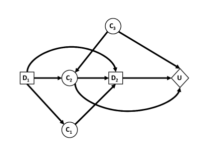
Figure 1: EF ID for our example

Table 2: Variables & relationships; plus $U$ as a function of $C_{3},D_{2}$ and $C_{2}$

$D_{1}$: Choice of treatment $C_{1}$: Initial reaction $C_{2}$: Response to treatment – $C_{2}\amalg C_{1}\ |\ D_{1}$ $D_{2}$: Decision on how to continue treatment $C_{3}$: Condition affecting response to treatment and medium-term health Can estimate $P(C_{3}\ |\ D_{1},C_{2})$ $U$: Medium-term health, a function of $C_{2},D_{2}$ and $C_{3}$        $C_{3}$ $C_{2}$ $D_{2}$ $U$ 1 1 1 $A$ 1 1 2 $A$ 1 2 1 $B$ 1 2 2 $C$ 2 1 1 $A$ 2 1 2 $A$ 2 2 1 $D$ 2 2 2 $E$

To avoid making the problem too complex for easy understanding we let all variables be binary except $U$, and introduce only two asymmetric features: So suppose that if a patient fails to respond to the first treatment ($C_{2}=1$), then the patient will inevitably have the lowest medium-term health rating ($U=A$). We can express this as $U\amalg(C_{3},D_{2})\ |\ (C_{2}=1)$ (see Table 2). Suppose also that if $D_{1}=2$ (Treatment 2 is given) then $C_{1}$ takes the value 1 (the patient’s body always accepts the treatment). The problem can be represented by the EF ID in Figure 1.

To express the asymmetry of the problem we can add distribution trees to the nodes $C_{1}$ and $U$ as in Figure 2. These have been drawn in a manner consistent with the other diagrams in this paper, rather than with those in [13].

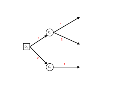
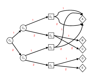
Figure 2: Distribution trees for nodes $C_{1}$ and $U$

The ID in Figure 1 is not the most parsimonious representation of the problem. If we can partition the parents of a decision node $D$ (those nodes with arrows into $D$) into two sets $Q^{A}(D),Q^{B}(D)$ such that $U\amalg Q^{B}(D)\ |\ (D,Q^{A}(D))$, then the set $Q^{B}(D)$ can be considered irrelevant for the purposes of maximising utility, and the edges from nodes in $Q^{B}(D)$ into $D$ can be removed from the ID. Here we find that $C_{1}\in Q^{B}(D_{2})$, and so the edge from $C_{1}$ to $D_{2}$ can be removed from the ID. The node $C_{1}$ is now barren, so it can also be removed (together with the edge $D_{1}\rightarrow C_{1}$).

Once we have our parsimonious ID we can use one of the standard solution methods to produce an optimal decision strategy and expected utility for this strategy. Using Shachter’s method (reversing the arc between $C_{3}$ and $C_{2}$, and adding a new arc from $D_{1}$ to $C_{3}$) we eventually get

$$U^{final}=\max_{D_{1}}\Big{[}\sum_{C_{2}}P(C_{2}\ |\ D_{1})\Big{[}\max_{D_{2}}\Big{[}\sum_{C_{3}}P(C_{3}\ |\ D_{1},C_{2})\ U(C_{2},C_{3},D_{2})\Big{]}\Big{]}\Big{]}$$

which does not however reflect the asymmetries in the problem. These can be built into the solution technique, but as the principal asymmetry concerns $U(C_{2},C_{3},D_{2})$, any advantage conveyed by the compactness of the ID is lost in the messy arithmetic.

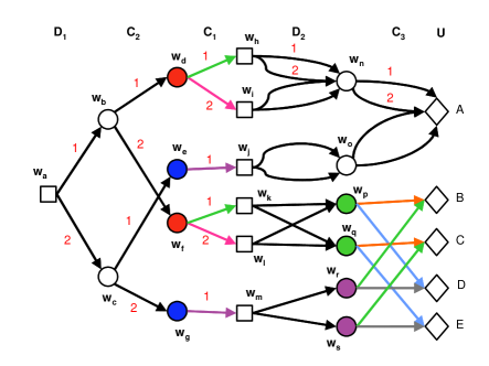
Figure 3: Initial EF CEG for our example

We now turn our attention to a CEG-representation of the problem. There are two EF orderings of the variables: $D_{1},C_{2},C_{1},D_{2},C_{3},U$ and one where $C_{1}$ & $C_{2}$ are interchanged. Note that $D_{2}$ precedes $C_{3}$ since the value of $C_{3}$ is not known to the DM when she comes to make a decision at $D_{2}$. The first ordering leads to a slightly more transparent graph.

As we are comparing CEGs and IDs here, we do not put any utilities onto edges, but restrict them to terminal utility nodes. We also separate out our single utility node into distinct utility nodes for each value taken by $U$. In more complex decision problems this can lead to greater transparency. We have elsewhere called this form of CEG without utilities on edges, and with separated utility nodes, a Type 2 decision CEG. The Type 2 CEG for the ordering $D_{1},C_{2},C_{1},D_{2},C_{3},U$ is given in Figure 3.

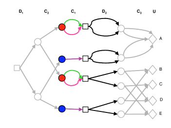
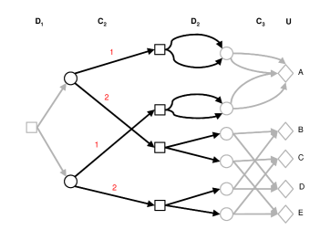
Figure 4: First and second simplifications

Conditional independence structure in a CEG can be read from individual positions, from stages, and from cuts through these [14]. Recall that nodes in the underlying tree are coalesced into positions when the sets of complete future developments from each node are the same and have the same probability distribution. So for example, the position $w_{n}$ yields the information that

$$(C_{3},U) \amalg(C_{1},D_{2})\ |\ (D_{1}=1,C_{2}=1) (3.1)$$

The position $w_{p}$ similarly yields $(C_{3},U)\amalg C_{1}\ |\ (D_{1}=1,C_{2}=2,D_{2}=1)$.

Recall that positions in a CEG are in the same stage if their sets of outgoing edges carry the same labels and have the same probability distribution. The positions $w_{p}$ & $w_{q}$ are in the same stage (indicated by the colouring), and so the probabilities on the edges leaving these positions have the same distibution, and hence

$$C_{3} \amalg(C_{1},D_{2})\ |\ (D_{1}=1,C_{2}=2) (3.2)$$

The expressions (3.1) & (3.2) result from the fact that in our EF CEG ordered $D_{1},C_{2},C_{1},D_{2},C_{3},U$, the variable $C_{3}$ is dependent on $D_{1}$ and $C_{2}$. This is not clear from the ID in Figure 1, but is reflected in the expression for $U^{final}$. But the form of this expected utility expression is a consequence of the arc-reversal required for successful ID-based solution of our problem. So this arc-reversal is already explicitly represented in the original EF CEG, and is not (as with IDs) an additional requirement of the solution technique.

A cut through a CEG is a set of positions or stages which partitions the set of root-to-sink/leaf paths. So the set of positions $\{w_{n},w_{o},w_{p},w_{q},w_{r},w_{s}\}$ is a cut of our CEG. A conditional independence statement associated with a cut is the union of those statements associated with the component positions (or stages) of the cut. So the cut through $\{w_{n},w_{o},w_{p},w_{q},w_{r},w_{s}\}$ gives us that

$$U \amalg C_{1}\ |\ (D_{1},C_{2},D_{2})$$

which is clearly of the form $U\amalg Q(D_{2}^{B})\ |\ (D_{2},Q(D_{2}^{A}))$, and tells us that $C_{1}$ is irrelevant to $D_{2}$ for the purposes of maximising utility.

For a Type 2 CEG drawn in EF order, two (or more) decision nodes are in the same position if the sub-CEGs rooted in each decision node have the same topology, equivalent edges in these sub-CEGs have the same labels & (where appropriate) probabilities, and equivalent branches terminate in the same utility node. So in Figure 3, the nodes $w_{h}$ & $w_{i}$ are in the same position, as are the nodes $w_{k}$ & $w_{l}$. Decision nodes in the same position can simply be coalesced, giving us the first graph in Figure 4.

For a Type 2 EF decision CEG with all positions coalesced (as in this graph), a barren node is simply a position $w$ for which $ch(w)$ (defined as in section 2) contains a single element. Barren nodes can be deleted in a similar manner to those in BNs – see Table 3 (where $pa(w)$ denotes the set of parent nodes of $w$).

Table 3: Barren node deletion algorithm (Type 2 decision CEGs)

• Choose a topological ordering of the positions excluding the terminal utility nodes: $w_{1},w_{2},\ldots,w_{m}$, such that $w_{1}$ is the root-node.

• Iterate: for $i=2$ step plus 1 until $i=m$ do:

  • If $ch(w_{i})$ contains only one node then Label this node $w_{\succ i}$ For each node $w_{\prec i}\in pa(w_{i})$ Replace all edges $e(w_{\prec i},w_{i})$ by a single edge $e(w_{\prec i},w_{\succ i})$ Delete all edges $e(w_{i},w_{\succ i})$ & the node $w_{i}$.

Four iterations of the algorithm applied to the first graph in Figure 4 yield the second graph in Figure 4. Further iterations will remove the first two $D_{2}$ nodes and the first two $C_{3}$ nodes to give the parsimonious CEG in Figure 5.

We can clearly see that $C_{1}$ is irrelevant for maximising $U$, and moreover if $C_{2}=1$ then both $D_{2}$ and $C_{3}$ are also irrelevant for this purpose (so the DM actually only needs to make one decision in this context). This latter property of the problem is not one that can be deduced from an ID-representation, although it could with some effort be worked out from the second distribution tree in Figure 2. It is however obvious in the parsimonious CEG.

Solution follows the method described in section 2 (the process obviously being simpler as there are no rewards or costs on the edges), and results in the expression

$$U^{final} =$$

$$\max\big{[} P(C_{2}=1\ |\ D_{1}=1)U_{A}+P(C_{2}=2\ |\ D_{1}=1)\times$$

$$\max\big{[} P(C_{3}=1\ |\ D_{1}=1,C_{2}=2)U_{B}+P(C_{3}=2\ |\ D_{1}=1,C_{2}=2)U_{D},$$

$$P(C_{3}=1\ |\ D_{1}=1,C_{2}=2)U_{C}+P(C_{3}=2\ |\ D_{1}=1,C_{2}=2)U_{E}\big{]},$$

$$P(C_{2}=1\ |\ D_{1}=2)U_{A}+P(C_{2}=2\ |\ D_{1}=2)\times$$

$$\max\big{[} P(C_{3}=1\ |\ D_{1}=2,C_{2}=2)U_{B}+P(C_{3}=2\ |\ D_{1}=2,C_{2}=2)U_{D},$$

$$P(C_{3}=1\ |\ D_{1}=2,C_{2}=2)U_{C}+P(C_{3}=2\ |\ D_{1}=2,C_{2}=2)U_{E}\big{]}\big{]}$$

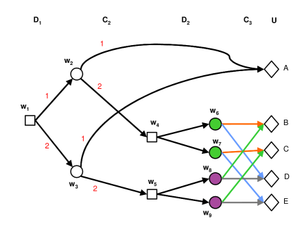
Figure 5: Parsimonious CEG

This expression is obviously more complex than that for the ID, but it is much more robust since it has been produced using the asymmetry of the problem to power the analysis, rather than treating it as an added complication.

4 Discussion

In this paper we have concentrated on how CEGs compare with IDs for the analysis of asymmetric decision problems. It is however worth pointing out two advantages of CEGs over coalesced trees: Firstly, the ability to read conditional independence structure from CEGs allowed us to create an analogue of the parsimonious ID, and secondly, the explicit representation of stage structure in CEGs gave rise to our barren node deletion algorithm.

A paper providing a more detailed discussion of parsimony, barren node deletion and arc reversal as they relate to CEGs is imminent. This paper will also provide a comparison of CEGs with VNs, SDDs and augmented IDs through a worked example. A further paper on the use of decision CEGs for multi-agent problems and games is also in the pipeline.

Acknowledgement: This research is being supported by the EPSRC (project EP/M018687/1).

References

- [1] Barclay L. M., Hutton J. L., and Smith J. Q. (2013) Refining a Bayesian Network using a Chain Event Graph, International Journal of Approximate Reasoning, 54:1300–1309.
- [2] Bhattacharjya D. and Shachter R. D. (2012) Formulating asymmetric decision problems as decision circuits, Decision Analysis, 9:138–145.
- [3] Bielza C. and Shenoy P. P. (1999) A comparison of graphical techniques for asymmetric decision problems, Management Science, 45:1552–1569.
- [4] Call H. J. and Miller W. A. (1990) A comparison of approaches and implementations for automating Decision analysis, Reliability Engineering and System Safety, 30:115–162.
- [5] Covaliu Z. and Oliver R. M. (1995) Representation and solution of decision problems using sequential decision diagrams, Management Science, 41(12).
- [6] Dawid A. P. (1979) Conditional independence in statistical theory, Journal of the Royal Statistical Society, Series B, 41:1–31.
- [7] Dawid A. P. (2012) The decision-theoretic approach to causal inference. In C. Berzuini, A. P. Dawid, and L. Bernardinelli, editors, Causality: Statistical Perspectives and Applications, pages 25–42. Wiley.
- [8] Jensen F. V., Nielsen T. D., and Shenoy P. P. (2006) Sequential influence diagrams: A unified asymmetry framework, International Journal of Approximate Reasoning, 42:101–118.
- [9] Qi R., Zhang N., and Poole D. (1994) Solving asymmetric decision problems with influence diagrams. In Proceedings of the 10th Conference on Uncertainty in Artificial Intelligence, pages 491–499.
- [10] Shachter R. D. (1986) Evaluating Influence diagrams, Operations Research, 34(6):871–882.
- [11] Shenoy P. P. (1996) Representing and solving asymmetric decision problems using valuation networks. In D. Fisher and H-J. Lenz, editors, Learning from Data: Artificial Intelligence and Statistics V. Springer-Verlag.
- [12] Silander T. and Leong T-Y. (2013) A Dynamic Programming Algorithm for Learning Chain Event Graphs. In Discovery Science, volume 8140 of Lecture Notes in Computer Science, pages 201–216. Springer.
- [13] Smith J. E., Holtzman S., and Matheson J. E. (1993) Structuring conditional relationships in influence diagrams, Operations Research, 41:280–297.
- [14] Smith J. Q. and Anderson P. E. (2008) Conditional independence and Chain Event Graphs, Artificial Intelligence, 172:42–68.
- [15] Thwaites P. A. (2013) Causal identifiability via Chain Event Graphs, Artificial Intelligence, 195:291–315.
- [16] Thwaites P. A., Smith J. Q., and Riccomagno E. M. (2010) Causal analysis with Chain Event Graphs, Artificial Intelligence, 174:889–909.