The Ba_0.6K_0.4Fe₂As₂ superconducting four-gap temperature evolution: a multi-band Chebyshev-BdG approach

Abstract

We generalize the Chebyshev-Bogoliubov-deGennes method to treat multi-band systems to address the temperature dependence of the superconducting (SC) gaps of iron based superconductors. Four SC gaps associated with different electron and hole pockets of optimally doped Ba_0.6K_0.4Fe₂As₂ were clearly identified by angle resolved photo-emission spectroscopy. The few approaches that reproduces with success this gap structure are based on strong-coupling theories and required many adjustable parameters. We show that an approach with a redistribution of electron population between the hole and electron pockets $\nu$ with evolving temperature reproduces the different coupling ratios $2\Delta^{\nu}(0)/k_{\rm B}T_{c}$ in these materials. We define the values that fit the four zero temperature gaps $\Delta^{\nu}(0)$ and after that all $\Delta^{\nu}(T)$ is obtained without any additional parameter.

I Introduction

Iron based high-$T_{c}$ superconductors (FeSCs) have been intensely studied, but there are still many fundamental open question concerning their mechanism of pairing. The main difficulty stems from their multi-band structure with indications of hybridisation among them. In this complex context, the strength of the electron-electron correlation is an issue of debate and this is one of the main points addressed here. The temperature dependence of the SC gap often indicates the coupling regime of Cooper pairs. Conventional BCS superconductors are characterized by a weak-coupling strength ratio of $2\Delta(0)/k_{\rm B}T_{c}\approx 3.52$, whereas strongly correlated superconductors display much higher values. In the case of Ba_0.6K_0.4Fe₂As₂ a ratio of $\approx 7.5$ is observed in the $\alpha$, $\gamma$ and $\delta$ pockets, while a ratio of $\approx 3.7$ is seen in the $\beta$ pocket at the Fermi surface Ding et al. (2008); Terashima et al. (2009); Nakayama et al. (2008). However, it is still unclear whether the strenght of the electron-electron interaction in the FeSCs is the cause of such high coupling ratios.

Despite the clear distinction of four different SC band-gaps Nakayama et al. (2008), optimally doped Ba_0.6K_0.4Fe₂As₂ displays a single critical temperature $T_{c}=37$ K. According to a well known result, this is a signal that the bands have an inter-dependent dynamics Suhl et al. (1959). The different coupling strength ratios $2\Delta^{\nu}(0)/k_{\rm B}T_{c}$ in the FeSCs are frequently interpreted as a coexistence of different coupling regimes Richard et al. (2011, 2015). It is not intuitive that bands originated from different iron $d$-orbitals would possess distinct regimes.

To deal with this problem we develop a generalization of the Chebyshev-Bogoliubov-deGennes (CBdG) method Covaci et al. (2010) to treat multi-band systems. This weak-coupling mean-field approach reproduces the four-gap structure in Ba_0.6K_0.4Fe₂As₂, by allowing the electron population to redistribute among the bands with evolving temperature. We show that bands with monotonically varying electron population with temperature can generate high coupling strength ratios $2\Delta^{\nu}(0)/k_{\rm B}T_{c}$ in multi-band systems, as would be expected in strong-coupling systems. After fitting the values of $\Delta^{\nu}(0)$, our theory reproduces the temperature evolution of the four $\Delta^{\nu}(T)$ exactly as in BCS, without introducing any new parameters. Then we show that a typical gap dependence $\Delta(T)$ is obtained by following a geodesic of constant chemical potential $\mu$ on the surface of $\Delta(\mu,T)$. The main point tackled in this paper shows that the four-gap structure of Ba_0.6K_0.4Fe₂As₂ is reproduced by geodesics on the surface of $\Delta(\mu,T)$, where $\mu=\mu(T)$. Whereas $\mu(T)$ varies monotonically for each band (and hence also the band population) the total density of the system is constant.

II The model

While in the cuprates the low-energy physical properties are captured by a single band, it is generally believed that a minimal model for the FeSCs must include all five $3d$ orbitals of iron Hirschfeld et al. (2011). It has been shown that the charge excitations in different orbitals can be decoupled, so that it can be effectively described by a collection of doped Hubbard-like Hamiltonians, each with a different electron population De Medici et al. (2014). As mentioned, angle resolved photo-emission spectroscopy (ARPES) on Ba_0.6K_0.4Fe₂As₂ measures four SC bands labeled $\alpha$, $\beta$, $\gamma$ and $\delta$ at the Fermi surface Nakayama et al. (2008).

Here we address only these four bands because our main goal is to reproduce their SC gap temperature dependence and, in doing so, obtain some insights on the paring mechanism. To set the CBdG method for the Ba_0.6K_0.4Fe₂As₂, we model each SC band by a square lattice, where each site represents a single decoupled orbital of Fe. Therefore, we model the Fe square lattice by four square lattices (sheets), each corresponding to a single band composed of decoupled $3d$ orbitals. This brings about a scenario where different pairing potentials may coexist. Inter-bands scattering is included as a single-particle scattering among these sheets.

Table 1: Effective hopping parameters $t_{1}$ (nearest neighbor) and $t_{2}$ (next-nearest neighbor) consistent with APRES band dispersion fit Richard et al. (2011). $U_{0}$ is the on-site $s$-wave pairing potential used in the BdG calculations of $\Delta^{\nu}_{\mathbf{i}}$.

(meV)	$\bm{\alpha}$	$\beta$	$\gamma$	$\delta$
$t_{1}$	160	13	380	380
$t_{2}$	-52	42	800	800
$U_{0}$	227	52	1013	982

Our multi-band Bogoliubov-deGennes (BdG) Hamiltonian Möckli and de Mello (2015) is then composed by two parts, an intra-band and an inter-band component: $\mathcal{H}=\mathcal{H}_{\mathrm{intra}}+\mathcal{H}_{\mathrm{inter}}$, where

$$\begin{split}\mathcal{H}_{\mathrm{intra}}&=\sum_{\langle\mathbf{ij}\rangle,\nu,\sigma}t_{\mathbf{ij}}^{\nu}\,c^{\dagger}_{\mathbf{i}\nu\sigma}c_{\mathbf{i}\nu\sigma}-\sum_{\mathbf{i,\nu,\sigma}}\mu_{\nu}(T)\,c^{\dagger}_{\mathbf{i}\nu\sigma}c_{\mathbf{i}\nu\sigma}\\ &+\sum_{\mathbf{i},\nu}\left(\Delta_{\mathbf{i}}^{\nu}\,c^{\dagger}_{\mathbf{i}\nu\uparrow}c^{\dagger}_{\mathbf{i}\nu\downarrow}+\mathrm{h.c.}\right)\\ &+\sum_{\langle\mathbf{ij}\rangle,\nu}\left(\Delta_{\mathbf{ij}}^{\nu}\,c^{\dagger}_{\mathbf{i}\nu\uparrow}c^{\dagger}_{\mathbf{j}\nu\downarrow}+\mathrm{h.c.}\right),\end{split}$$ (1)

with

$$\Delta_{\mathbf{i}}^{\nu}=U_{\mathbf{i}}^{\nu}\langle c_{\mathbf{i}\nu\downarrow}c_{\mathbf{i}\nu\uparrow}\rangle,\quad\mbox{and}\quad\Delta_{\mathbf{ij}}^{\nu}=U_{\mathbf{ij}}^{\nu}\langle c_{\mathbf{j}\nu\downarrow}c_{\mathbf{i}\nu\uparrow}\rangle,$$ (2)

describes the intra-band dynamics, where the band index $\nu$ runs over the $\alpha$, $\beta$, $\gamma$ and $\delta$ band. The $t_{\mathbf{ij}}^{\nu}$ are intra-band hoppings between lattice sites $\mathbf{i}$ and $\mathbf{j}$ up to second nearest neighbors as derived by ARPES band dispersion tight-binding fit Richard et al. (2011); see table 1. The temperature dependent band chemical potential $\mu_{\nu}(T)$ allows for self-consistent regulation of the band fillings with temperature evolution. The local gap amplitude $\Delta_{\mathbf{i}}^{\nu}$ realizes a constant $s$-wave gap. The non-local gap amplitudes $\Delta_{\mathbf{ij}}^{\nu}$, which can be nearest or next-nearest neighbors, realize unconventional gap symmetries.

Single particle inter-sheet scattering is usually described by Zhang et al. (2014); Balatsky et al. (2006)

$$\mathcal{H}_{\mathrm{inter}}=\sum_{\langle\mathbf{ij}\rangle,\mu\neq\nu,\sigma}\left(V_{\mathbf{ij}}^{\mu\nu}c^{\dagger}_{\mathbf{i}\mu\sigma}c_{\mathbf{j}\nu\sigma}+\mathrm{h.c.}\right),$$ (3)

where $V_{\mathbf{ij}}^{\mu\nu}$ is a non-local (nearest-neighbor) scattering potential among the bands and causes the multi-gaps to vanish at a common critical temperature $T_{c}=37$ K Möckli and de Mello (2015); Suhl et al. (1959). The scattering strength is strong between bands close in momentum space (low momentum transfer), and weak for distant bands (high momentum transfer) Zhang et al. (2014). Taking this into account, we use $V^{\alpha\beta}=V^{\gamma\delta}=100$ meV and neglect all other distant bands scatterings.

III The multi-band CB$\rm d$G method

As it is common to BdG method, we determine self consistently the gap-functions $\Delta_{\mathbf{i}}^{\nu}$ and $\Delta_{\mathbf{ij}}^{\nu}$, the local density of states (LDOS) $\rho_{\mathbf{i}}$, and the local density $n_{\mathbf{i}}$ (the sum of all sheet populations). To do so, we generalize the Chebyshev-BdG (CBdG) method Covaci et al. (2010) to determine the real-space time-ordered Nambu-Gor’kov Green’s function of a multi-band superconductor. The CBdG method is an efficient numerical method generally applied to inhomogeneous superconductors, where exact diagonalization techniques impose severe restrictions on system’s sizes. Here, we take advantage of the CBdG method to investigate homogeneous multi-band superconductors; thereby circumventing the limitations imposed by the size of the matrix Hamiltonian of multi-band materials. We outline the basic steps below; for more details we refer the reader to reference Weisse et al. (2006).

We write the double-time Green’s function for band $\nu$ as

$$G_{\mathbf{ij}}^{\nu}(t,0)=-\frac{i}{\hbar}\begin{bmatrix}\langle\mathcal{T}c_{\mathbf{i}\nu\uparrow}(t)c^{\dagger}_{\mathbf{j}\nu\uparrow}(0)\rangle&\langle\mathcal{T}c_{\mathbf{i}\nu\uparrow}(t)c_{\mathbf{j}\nu\downarrow}(0)\rangle\\ \langle\mathcal{T}c^{\dagger}_{\mathbf{i}\nu\downarrow}(t)c^{\dagger}_{\mathbf{j}\nu\uparrow}(0)\rangle&\langle\mathcal{T}c^{\dagger}_{\mathbf{i}\nu\downarrow}(t)c_{\mathbf{j}\nu\downarrow}(0)\rangle\end{bmatrix},$$ (4)

where $\mathcal{T}$ is the time-ordering operator and $\langle\ldots\rangle$ are thermal-averages. One can rewrite equation (4) with energy arguments as

$$G_{\mathbf{ij}}^{\nu}(E)=\begin{bmatrix}\langle c_{\mathbf{i}\nu\uparrow}|G(E)|c^{\dagger}_{\mathbf{j}\nu\uparrow}\rangle&\langle c_{\mathbf{i}\nu\uparrow}|G(E)|c_{\mathbf{j}\nu\downarrow}\rangle\\ \langle c^{\dagger}_{\mathbf{i}\nu\downarrow}|G(E)|c^{\dagger}_{\mathbf{j}\nu\uparrow}\rangle&\langle c^{\dagger}_{\mathbf{i}\nu\downarrow}|G(E)|c_{\mathbf{j}\nu\downarrow}\rangle\end{bmatrix},$$ (5)

where

$$G(E)=\lim_{\eta\rightarrow 0}\frac{1}{E-\mathcal{H}+i\eta},$$ (6)

and $\eta$ is a positive infinitesimal. For an L$\times$ L square lattice and b bands, the matrix representation of $\mathcal{H}$ has dimension 2bL². Here we use b=4 and L=30. In our calculations no significant changes were observed for $L>30$.

The diagonal ($\kappa=1$) and off-diagonal ($\kappa=2$) components of equation (5) – $G_{\mathbf{ij}}^{\nu,1\kappa}(E)$ – correspond to the normal and anomalous (superconducting) Green’s functions respectively. In order to expand these components in terms of orthogonal Chebyshev polynomials, we must rescale energy related quantities as $\tilde{E}=(E-b)/a$, where $a=(E_{\mathrm{max}}-E_{\mathrm{min}})/(2-\epsilon)$ and $b=(E_{\mathrm{max}}-E_{\mathrm{min}})/2$, where $\epsilon$ is a small cutoff to avoid stability problems. $E_{\mathrm{max}}$ and $E_{\mathrm{max}}$ are estimates of the bounded extremal values of the eigenvalue spectra of the Hamiltonian. Since we treat a homogeneous system, these estimates can be exactly obtained by diagonalizing a much smaller version of the full $\rm 2{bL}^{2}\times 2{bL}^{2}$ matrix. The Hamiltonian operator rescales as $\tilde{\mathcal{H}}=(\mathcal{H}-b\mathbb{1})/a$. We indicate all rescaled quantities with a tilde thereafter.

The components of the Green’s function (5) can be expanded in terms of orthogonal Chebyshev polynomials, which we write as

$$\tilde{G}_{\mathbf{ij}}^{\nu,1\kappa}(\tilde{E})=-\frac{i}{\sqrt{1-\tilde{E}^{2}}}\sum_{n=0}^{N}\mu_{\mathbf{ij}}^{\nu,1\kappa}(n)\,e^{-in{\rm arccos}(\tilde{E})},$$ (7)

where the expansion moments are given by

$$\mu_{\mathbf{ij}}^{\nu,11}(n)=\frac{2}{1+\delta_{n,0}}\langle c_{\mathbf{i}\nu\uparrow}|T_{n}(\tilde{\mathcal{H}})|c^{\dagger}_{\mathbf{j}\nu\uparrow}\rangle,$$ (8)

$$\mu_{\mathbf{ij}}^{\nu,12}(n)=\frac{2}{1+\delta_{n,0}}\langle c^{\dagger}_{\mathbf{i}\nu\downarrow}|T_{n}(\tilde{\mathcal{H}})|c^{\dagger}_{\mathbf{j}\nu\uparrow}\rangle.$$ (9)

In this paper only these two components are necessary. We calculate the moments up to expansion order $n=3000$. The expansion (7) must be convoluted with a proper kernel in order to damp the resulting Gibbs oscillations originating from the Chebyshev polynomials $T_{n}(\mathcal{\tilde{H}})$. To do so we use the Lorentz kernel, which is designed for Green’s functions Weisse et al. (2006). The Chebyshev matrix polynomials $T_{n}(\tilde{\mathcal{H}})$ obey the recurrence relation

$$T_{n+1}(\tilde{\mathcal{H}})=2\,\tilde{\mathcal{H}}\,T_{n}(\tilde{\mathcal{H}})-T_{n-1}(\tilde{\mathcal{H}}).$$ (10)

Using equation (10), the expansion moments (8) and (9) are obtained by an efficient and stable iterative procedure involving repeated applications of the rescaled Hamiltonian via (10) on iterative vectors $|c^{\dagger}_{\mathbf{j}\nu\uparrow}\rangle$. The diagonal moments (8) are used to calculate the local density of states (LDOS)

$$\tilde{\rho}_{\mathbf{i}}^{\uparrow(\downarrow)}=-\frac{1}{\pi}\sum_{\nu}\mathrm{Im}\,\tilde{G}_{\mathbf{ii}}^{\nu,11(22)}(\tilde{E}).$$ (11)

For no external magnetic fields $\tilde{\rho}_{\mathbf{i}}^{\uparrow}=\tilde{\rho}_{\mathbf{i}}^{\downarrow}$, such that $\tilde{\rho}_{\mathbf{i}}=2\tilde{\rho}_{\mathbf{i}}^{\uparrow}$. A final back-scaling yields $\rho_{\mathbf{i}}$. The local charge density is determined by

$$n_{\mathbf{i}}=\int_{-1}^{1}\mathrm{d}\tilde{E}\,\tilde{\rho}_{\mathbf{i}}(\tilde{E})\tilde{f}(\tilde{E}),$$ (12)

where the integral is performed in the Chebyshev interval $[-1,1]$ and $\tilde{f}(\tilde{E})$ is the rescaled Fermi distribution. Such integrals can be efficiently calculated using Chebyshev-Gauss techniques Weisse et al. (2006).

The off-diagonal moments (9) determine the temperature dependence of the real part of the superconducting gaps

$$\Delta_{\mathbf{i}}^{\nu}(T)=\frac{|U^{\nu}_{\mathbf{i}}|}{2\pi}\int_{-1}^{1}\mathrm{d}\tilde{E}\,\mathrm{Im}\,\tilde{G}_{\mathbf{ii}}^{\nu,12}(\tilde{E})\tanh\left(\frac{\tilde{E}}{2\tilde{k}_{B}T}\right);$$ (13)

$$\Delta_{\mathbf{ij}}^{\nu}(T)=\frac{|U^{\nu}_{\mathbf{ij}}|}{2\pi}\int_{-1}^{1}\mathrm{d}\tilde{E}\,\mathrm{Im}\,\tilde{G}_{\mathbf{ij}}^{\nu,12}(\tilde{E})\tanh\left(\frac{\tilde{E}}{2\tilde{k}_{B}T}\right).$$ (14)

Figure 1: Real space superconducting gap profiles with an underlining square lattice (black dots) correspondent to the gap structures: $s$-wave $\Delta(k_{x},k_{y})\propto\mathrm{const.}$ (upper-left panel), $s$-wave $\Delta(k_{x},k_{y})\propto\cos{k_{x}}+\cos{k_{y}}$ (upper-right panel), $d$-wave $\Delta(k_{x},k_{y})\propto\cos{k_{x}}-\cos{k_{y}}$ (lower-left panel), and $s$-wave $\Delta(k_{x},k_{y})\propto\cos{k_{x}}\cos{k_{y}}$ (lower-right panel). Lighter colors correspond to higher gap values. The upper-left and lower-right panels show the most likely candidates to describe the FeSCs.

For a homogeneous system, we need the list $\{\mu_{\mathbf{ii}}^{\nu,11}(n)\}$ with $\nu=\alpha,\beta,\gamma,\delta$ to calculate the density of states (DOS) from (11), for any $\mathbf{i}$. Similarly, the constant local $s$-wave gap is determined from the list $\{\mu_{\mathbf{ii}}^{\nu,12}(n)\}$, and the nearest neighbor and next-nearest neighbor gaps $\Delta_{\mathbf{ij}}$ are extracted from the list $\{\mu_{\mathbf{ij}}^{\nu,12}(n)\}$ for any fixed $\mathbf{i}$.

Different combinations of the gap functions (14) emulate a menu of gap symmetries in $\mathbf{k}$-space. In table 2 we show the correspondence of four well-known gap structures in momentum space, with its counterpart in lattice space. To understand the form of the lattice-space combinations, we show the real space profile – the Fourier transformed momentum gap structures – with an underlining square lattice in figure 1. To determine the local unconventional gap value, we take the mean value of the inter-site gap profile Soininen et al. (1994); Schmid et al. (2010), see table 2.

Table 2: Correspondence between different gap structures in momentum space and lattice space. The vector $\mathbf{x}$ ($\mathbf{y}$) connects two neighboring horizontal (vertical) lattice sites. The vector $\mathbf{d}=\mathbf{x}+\mathbf{y}$ and $\mathbf{g}=\mathbf{y}-\mathbf{x}$.

$\mathbf{k}$-space	Lattice space
const.	$\Delta_{\mathbf{i}}=\Delta_{\mathbf{i}}$
$\cos k_{x}+\cos k_{y}$	$\Delta_{\mathbf{i}}=(\Delta_{\mathbf{i},\mathbf{i}+\mathbf{x}}+\Delta_{\mathbf{i},\mathbf{i}-\mathbf{x}}+\Delta_{\mathbf{i},\mathbf{i}+\mathbf{y}}+\Delta_{\mathbf{i},\mathbf{i}-\mathbf{y}})/4$
$\cos k_{x}-\cos k_{y}$	$\Delta_{\mathbf{i}}=(\Delta_{\mathbf{i},\mathbf{i}+\mathbf{x}}+\Delta_{\mathbf{i},\mathbf{i}-\mathbf{x}}-\Delta_{\mathbf{i},\mathbf{i}+\mathbf{y}}-\Delta_{\mathbf{i},\mathbf{i}-\mathbf{y}})/4$
$\cos k_{x}\cos k_{y}$	$\Delta_{\mathbf{i}}=(\Delta_{\mathbf{i},\mathbf{i}+\mathbf{d}}+\Delta_{\mathbf{i},\mathbf{i}-\mathbf{d}}+\Delta_{\mathbf{i},\mathbf{i}+\mathbf{g}}+\Delta_{\mathbf{i},\mathbf{i}-\mathbf{g}})/4$

IV Temperature dependence of the four-gap structure

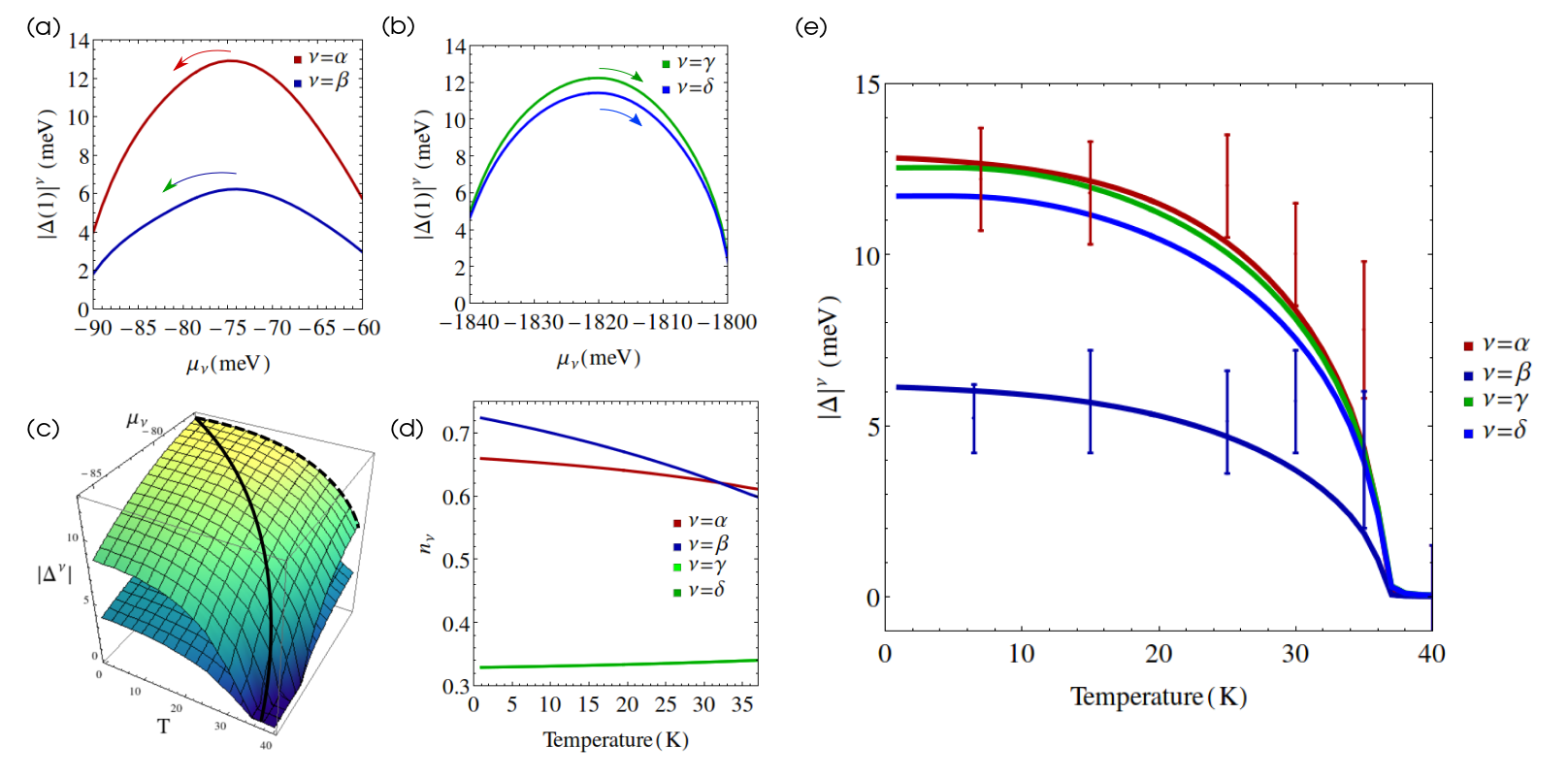
Figure 2: (a) Behavior of the superconducting gap in the $\alpha$ and $\beta$ bands with varying chemical potential. A monotonic loss (or gain) in intra-band electron population causes higher coupling ratios than the usual BCS result of $2\Delta/k_{\rm B}T\approx 3.52$. The red and the blue arrows indicate the direction of the chemical potential when temperature increases. This implies a monotonic reduction of electron population in the $\alpha$ and $\beta$ bands. See figure c for the 3D version. (b) The gaps in the $\gamma$ and $\delta$ bands as a function of the chemical potential. To conserve the total electron population, the $\gamma$ and $\delta$ bands gain electrons as indicated by the green and blue arrows. (c) The surface of $\Delta^{\alpha}(\mu_{\alpha},T)$ above with the the surface of $\Delta^{\beta}(\mu_{\beta},T)$ beneath. The dashed line shows the constant $\mu$ BCS-geodesic $\Delta^{\alpha}(-76,T)$. The solid line shows a geodesic with varying chemical potential, with initial point at $\Delta^{\alpha}(-76,1)$ and final point at $\Delta^{\alpha}(-84.5,37)$, that reproduces the temperature dependence of the energy gaps in FeSCs. Geodesics for the other bands are similar. (d) Redistribution of electron population among the superconducting bands with temperature along the four geodesics. In the present case, $\alpha$ and $\beta$ bands loose electrons, while $\gamma$ and $\delta$ bands gain electrons. The $\gamma$ and $\delta$ curves coincide. (e) Projections of the four geodesics onto the $\Delta^{\nu}(T)$ plane. We show error bars as extracted from ARPES for the $\alpha$ and $\beta$ band-gaps. The gap in $\gamma$ almost coincides with $\alpha$, and experimental points for the $\delta$-gap were not available.

We examine the case of constant local $s$-wave superconductivity in equation (13), that is, $U_{\mathbf{i}}^{\nu}=\mathrm{const.}$ and all $U_{\mathbf{ij}}^{\nu}=0$; see table 1. Weak-coupling BCS multi-band models cannot simultaneously reproduce the experimental values of the superconducting critical temperature and energy gaps, because they yield coupling rations $2\Delta/k_{B}T_{c}\approx 3.52$. A BCS-like temperature dependence of the energy gap has constant chemical potential $\Delta^{\nu}(T)\equiv\Delta^{\nu}(\mu=\mathrm{const},T)$. This is certainly the case in single-band systems such as the cuprates, where band filling remains constant. However, the FeSCs are intrinsically multi-band systems – the total electron population $n=\sum_{\nu}n_{\nu}$ is fixed, but band electron population $n_{\nu}(T)$ may vary, and hence $\mu_{\nu}(T)$. This opens the possibility that $\Delta^{\nu}(T)$ may be a geodesic over the surface of $\Delta^{\nu}(\mu_{\nu},T)$, in which the chemical potential $\mu$ is allowed to vary monotonically in a specific band in contrast to the BCS-like constant $\mu$ geodesic over $\Delta^{\nu}(\mu,T)$, see figure 2c. To show how the energy gap varies with electron population, we plot $\Delta^{\nu}(\mu,1)$ in figure 2a and figure 2b for $\nu=\alpha,\beta$ and $\nu=\beta,\gamma$ respectively. We call attention to the peaks of the gap intensity in $\alpha$ and $\beta$ bands at $\mu_{\alpha,\beta}=-76$ meV that have correspondent electron populations of $n_{\alpha}=0.66$ and $n_{\beta}=0.72$. These band populations can be extracted from the components of equation (11). Simultaneously, the gaps in the $\gamma$ and $\delta$ bands peak at $\mu_{\gamma,\delta}=-1820$ meV, which is consistent with their smaller band population $n_{\gamma,\delta}=0.33$; consistent with pocket sizes as observed by ARPES Richard et al. (2011, 2015).

Our main calculation is explained in figure 2 where the calculated $\Delta^{\nu}(\mu,T)$ follows a geodesic to left (red and blue arrows in figure 2a) of the peak in the $\alpha$ and $\beta$ hole bands, while $\Delta^{\nu}(\mu,T)$ in the $\gamma$ and $\delta$ bands follow a geodesic to the right (green and light-blue arrows in figure 2b) on their correspondent peaks. The paths must be different to conserve the total density of the multi-band system. This allows for high coupling ratios caused by a redistribution of electron population among the bands with varying temperature. While electron population increases in the $\alpha$ and $\beta$ bands with increasing temperature, electron population decreases at the same rate in the $\gamma$ and $\delta$ bands, thus maintaining the total density of the system constant; see figure 2d.

In figure 2c we show the geodesic on the $\Delta^{\alpha}(\mu,T)$ surface to illustrate the idea, which is analogous for the other surfaces. In figure 2e we plot our main results, the projections of the four geodesics on the four $\Delta^{\nu}(\mu,T)$-surfaces. These projections reproduce the experimental superconducting gap dependence with temperature. Unfortunately, little experimental data is available for optimally doped Ba_1-xK_xFe₂As₂. The experimental error bars we show in figure 2e are one of the earliest papers on the temperature dependence of the multi-gap structure in these materials Ding et al. (2008). However, by studying the temperature dependence of the energy gaps for other dopings, it is generally accepted that the formula $\Delta^{\nu}(T)=\Delta^{\nu}(0)\tanh(\pi/2\sqrt{T_{c}/T-1})$ fits the experimental in the FeSCs Evtushinsky et al. (2009). Our theoretical CBdG curves coincide exactly with this empirical formula.

We also investigated the unconventional gap structure with $U_{\mathbf{i}}^{\nu}=0$ and non-zero second-nearset neigbors $U_{\mathbf{ij}}^{\nu}$, which emulates $\cos k_{x}\cos k_{y}$ gap symmetry in $\mathbf{k}$-space; see figure 1d. By properly readjusting the $U_{\mathbf{ij}}^{\nu}$ and slightly different chemical potentials, one can obtain similar results as obtained by the constant $s$-wave case following the same charge redistribution arguments as discussed above.

V Conclusion

We generalized the CBdG method to treat multi-band superconductors. This allowed us to evaluate $7200\times 7200$ ($\rm 2{bL}^{2}\times 2{bL}^{2}$) matrices, which would be unfeasible with the exact diagonalization BdG technique. We used the CBdG method’s efficiency to address four bands simultaneously, instead of studying inhomogeneous superconductivity.

We demonstrated that a multi-band BdG theory can reproduce at a single calculation the high and low coupling ratios $2\Delta/k_{\rm B}T_{c}$ observed in high-$T_{c}$ multi-band FeSCs. The central point of our theory is the SC calculations at the maxima of $\Delta^{\nu}(\mu,T)$ with slightly variation of $\mu(T)$ with the temperature (of the order of 10 - 20 meV). This represents a small exchange of particle between the overlaping bands $\alpha$ - $\beta$ and $\gamma$ - $\delta$. The calculated $\Delta^{\nu}(\mu,T)$ curves were in completely agreement with the empirical estimates of the experimental results. Surely these cannot be used for single-band superconductors such as the cuprates. A multi-band context is indispensable, where band electron populations can redistribute.

References

- Ding et al. (2008) H. Ding, P. Richard, K. Nakayama, T. Sugawara, T. Arakane, Y. Sekiba, A. Takayama, S. Souma, T. Sato, T. Takahashi, Z. Wang, X. Dai, Z. Fang, G. F. Chen, J. L. Luo, and N. L. Wang, EPL 83, 0295 (2008).
- Terashima et al. (2009) K. Terashima, Y. Sekiba, J. H. Bowen, K. Nakayama, T. Kawahara, T. Sato, P. Richard, Y.-M. Xu, L. J. Li, G. H. Cao, Z.-A. Xu, H. Ding, and T. Takahashi, Proc. Natl. Acad. Sci. U. S. A. 106, 7330 (2009).
- Nakayama et al. (2008) K. Nakayama, T. Sato, P. Richard, Y. M. Xu, Y. Sekiba, S. Souma, G. F. Chen, J. L. Luo, N. L. Wang, H. Ding, and T. Takahashi, EPL 85, 4 (2008).
- Suhl et al. (1959) H. Suhl, B. Matthias, and L. Walker, Phys. Rev. Lett. 3, 552 (1959).
- Richard et al. (2011) P. Richard, T. Sato, K. Nakayama, T. Takahashi, and H. Ding, Reports Prog. Phys. 74, 124512 (2011).
- Richard et al. (2015) P. Richard, T. Qian, and H. Ding, J. Phys. Condens. Matter 27, 293203 (2015).
- Covaci et al. (2010) L. Covaci, F. M. Peeters, and M. Berciu, Phys. Rev. Lett. 105, 167006 (2010).
- Hirschfeld et al. (2011) P. J. Hirschfeld, M. M. Korshunov, and I. I. Mazin, Reports Prog. Phys. 74, 124508 (2011).
- De Medici et al. (2014) L. De Medici, G. Giovannetti, and M. Capone, Phys. Rev. Lett. 112, 1 (2014).
- Möckli and de Mello (2015) D. Möckli and E. V. L. de Mello, EPL 109, 17011 (2015).
- Zhang et al. (2014) P. Zhang, P. Richard, T. Qian, X. Shi, J. Ma, L. K. Zeng, X. P. Wang, E. Rienks, C. L. Zhang, P. Dai, Y. Z. You, Z. Y. Weng, X. X. Wu, J. P. Hu, and H. Ding, Phys. Rev. X 4, 1 (2014).
- Balatsky et al. (2006) a. V. Balatsky, I. Vekhter, and J. X. Zhu, Rev. Mod. Phys. 78, 373 (2006).
- Weisse et al. (2006) A. Weisse, G. Wellein, A. Alvermann, and H. Fehske, Rev. Mod. Phys. 78, 275 (2006).
- Soininen et al. (1994) P. Soininen, C. Kallin, and A. Berlinsky, Phys. Rev. B 50, 13883 (1994).
- Schmid et al. (2010) M. Schmid, B. M. Andersen, A. P. Kampf, and P. J. Hirschfeld, New J. Phys. 12, 053043 (2010).
- Evtushinsky et al. (2009) D. V. Evtushinsky, D. S. Inosov, V. B. Zabolotnyy, M. S. Viazovska, R. Khasanov, A. Amato, H.-H. Klauss, H. Luetkens, C. Niedermayer, G. L. Sun, V. Hinkov, C. T. Lin, A. Varykhalov, A. Koitzsch, M. Knupfer, B. Büchner, A. A. Kordyuk, and S. V. Borisenko, New J. Phys. 11, 055069 (2009).