Experimental Study of Synchronization of Coupled Electrical Self-Oscillators and Comparison to the Sakaguchi-Kuramoto model

Abstract

We explore the collective phase dynamics of Wien-bridge oscillators coupled resistively. We carefully analyze the behavior of two coupled oscillators, obtaining a transformation from voltage to effective phase. From the phase dynamics we show that the coupling can be quantitatively described by Sakaguchi’s modification to the Kuramoto model. We also examine an ensemble of oscillators whose frequencies are taken from a flat distribution within a fixed frequency interval. We characterize in detail the synchronized cluster, its initial formation, as well as its effect on unsynchronized oscillators, all as a function of a global coupling strength.

I Introduction

The study of spontaneous synchronization is a rich and cross-disciplinary field of research. The phenomenon can be identified to play a crucial role in many real biological buck ; walker , chemical kiss ; fukuda ; solomon , and mechanical systems bridge ; mertens ; zhang , as well as in neuroscience michaels ; sompolinsky ; breakspear . Powerful mathematical tools kura ; sakaguchi ; kuramoto ; strogatz ; pikovsky-book ; OttAntonsen have been developed to analyze synchronization. In spite of the utility and breadth of the concept, the vast majority of empirical work on synchronization has been numerical: simple experimental testbeds are rare in the literature.

A number of complicated experimental systems have been shown to synchronize. Although some have seen use in testing theories of synchronization, most are experimentally less accessible. Experiments with pedestrians on the Millennium Bridge in London bridge are difficult to repeat (for obvious reasons). Lasers lasers , Josephson junctions josephson , nickel-electrodes submerged in sulfuric acid kiss , and Belousov-Zhabotinsky reactors bz-reactors require substantial experimental setup. Resonantly coupled cell-phone vibrators mertens push the limits of conventional synchronization theory but do not allow much control in the coupling. Arrays of Belousov-Zhabotinsky droplets bz-droplets only support 1D or 2D lattice topologies. The circuit of Bergner and coworkers along with that of Gambuzza et al. offers an implementation of electronic oscillators based on analog multipliers to model Stuart-Landau oscillators and neurons, respectively, but even these are complicated circuits bergner ; FHN-circuit . In many of these systems, the detailed time- and oscillator-resolved phase dynamics is difficult to capture experimentally, and the coupling network topology limited or essentially fixed.

In contrast to all of the given systems, the oscillator circuit of Temirbayev et al. is simple to build and flexibly couple rosenblum ; moro . The underlying circuit design is a Wien-bridge oscillator, an electronic implementation of a relaxation oscillator. Electronic oscillatory systems possess a number of advantages for testing theories of synchronization. They have near-perfect measurement accessibility. They are easy to prototype or to fabricate in bulk. The coupling between oscillators can be varied from all-to-all to lattice to complex network by merely rearranging wires. Wien-bridge oscillators can be made to exhibit phase-oscillator behavior with near-constant amplitude, even when coupled to other oscillators. As we will show in this paper, coupled Wien-bridge oscillators can be quantitatively modeled by the simple Sakaguchi-Kuramoto model sakaguchi .

This paper is structured as follows. In Section II, we describe the experimental system, detailing individual and coupled circuit designs. In Section III we present a series of measurements for a pair of coupled oscillators in which one oscillator’s uncoupled speed is increased with each measurement, and use this data to obtain a simple phase-oscillator model for our system. In Section IV we explore the synchronization dynamics of a system of 19 and 20 coupled oscillators in which the coupling topology is systematically altered, and present measurements of the transient approach to synchronization.

II Experimental system and setup

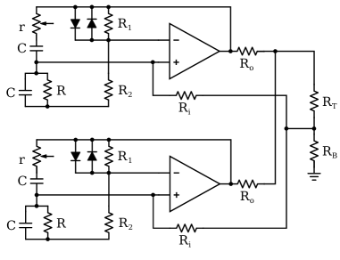
Figure 1: Circuit diagram of two coupled Wien-bridge oscillators. The intrinsic frequency is determined by the values of r, R and C. The resistor $R_{i}$ receives the voltage from the shared voltage divider, whereas the resistor $R_{o}$ transmits to the voltage divider. For our experiments we have $R_{1}=27\,\mbox{k$\Omega$}$, $R_{2}=3\,\mbox{k$\Omega$}$, $C=0.1\,\mbox{$\mu$F}$, $R=4.7\,\mbox{k$\Omega$}$, $r$ represents a $5\,\mbox{k$\Omega$}$ potentiometer, $R_{i}=62\,\mbox{k}\Omega$, and $R_{o}=1.1\,\mbox{k}\Omega$.

Figure 1 gives the circuit diagram of two Wien-bridge oscillators coupled to one another. We will first consider the circuit for uncoupled oscillators, obtained by removing the $R_{i}$ and $R_{o}$ resistors. Each oscillator principally consists of two branches, the resistor/capacitor branch and the resistor/diode branch, configured as a non-inverting amplifier. The resistor/capacitor branch sets the primary frequency of the oscillator, $\omega_{0}=\sqrt{\frac{1}{RrC^{2}}}$. We can easily change this frequency by altering the resistance of the potentiometer $r$, and we operate our oscillators between $200\,\mbox{Hz}$ and $400\,\mbox{Hz}$. The resistor/diode branch dictates the shape of the waveform and its sensitivity to perturbations. A pure but sensitive sine-wave results by setting the gain, $\left(R_{1}+R_{2}\right)/R_{2}$, to 3. To produce coupled oscillations with robust amplitudes, the gain for our setup is 10. The signal at such a high gain is far from sinusoidal, characterized by multiple harmonics, but the constant amplitude justifies treating them as phase oscillators.

The topology, direction, and nature of the coupling is highly configurable. In Fig. 1, two oscillators are coupled via two additional resistors for each oscillator, namely the $R_{o}$ output resistor and the $R_{i}$ input resistor rosenblum . This coupling method can then be easily extended to $N$ oscillators, as shown in Fig. 2. Connecting the oscillators to a common tank circuit would produce an experiment equivalent to the Millennium Bridge bridge . Connecting the oscillators to a tank circuit with two resonant frequencies would give an analog to the coupled rotors of Mertens and Weaver mertens . Connecting the oscillators in series using unity-gain buffers can produce a 1D nearest-neighbor lattice suitable for testing the renormalization theory of Lee et al. chain-universality , while purely resistive coupling would lead to non-local effects suitable for testing theories of chimeras chimera-theory . Complex network coupling could be used to test the coupling extraction methods of Kraleman et al. reconstructing-networks . Temirbayev et al. introduced additional electronics that led to a nonlinear shift in the phase coupling rosenblum . In this paper, we focus on a form of directed coupling in which all oscillators are influenced by a selected subset of the oscillators, which we call all-to-some coupling.

As shown in Fig. 2, the individual input resistors are all connected to a common bus, as are the individual output resistors. The coupling strength is determined by the settings of the voltage-divider resistors, $R_{B}$ and $R_{T}$, where we maintain the constraint $R_{B}+R_{T}=4\,\mbox{k$\Omega$}$. (To see why, notice that $R_{i}\gg R_{B}$ implies that the voltage drop across $R_{T}+R_{B}$ is the average of the oscillator output voltages. In that case, the mid-point between $R_{T}$ and $R_{B}$ serves as a simple voltage divider.) We have also included DIP switches, $S_{1}$ and $S_{2}$, at every oscillator’s input and the output, which serves both as a measurement convenience and as a simple means for changing which oscillators can effect and are effected by the common signal on the bus. With all switches closed, we obtain the conventional all-to-all coupling. By opening an oscillator’s $S_{1}$ and $S_{2}$, we isolate the oscillator and can measure its uncoupled behavior. By closing $S_{1}$ and $S_{2}$ for an individual oscillator and opening $S_{1}$ and $S_{2}$ for all other oscillators, we can measure the oscillator’s self-coupled behavior. Closing $S_{1}$ and $S_{2}$ for only two oscillators produces the pair-coupled configuration shown in Fig. 1. Finally, by closing $S_{1}$ for all oscillators and selectively opening $S_{2}$, we couple all oscillators to the common bus but choose which oscillators contribute to the common bus.

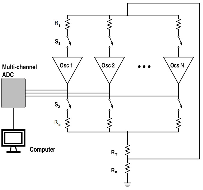
Figure 2: A schematic of the $N$ Wien-bridge oscillators. We incorporate two sets of switches, one to prevent particular oscillators from “talking”, and the other to prevent them from “listening” to the others. The oscillillators operate at frequencies between $200\,\mbox{Hz}$ and $400\,\mbox{Hz}$, and their voltages are sampled every $0.1\,\mbox{ms}$.

The voltages at the output of each oscillator are simultaneously digitized using a 14-bit multi-channel DAC with a time resolution of $0.1\,\mbox{ms}$. The data is streamed to and stored at an acquisition card of a computer. We trigger the measurement using a pulse generator. For some measurements where transients are recorded, the pulse generator also drives an analog switch (ADG 452B). This switch, when closed, bypasses resistor $R_{B}$ to ground and essentially turns the coupling strength to zero. Upon opening the switch, the coupling is abruptly turned on.

There are many frequencies that describe the behavior of these oscillators. In some of our measurements we will focus on the time series of frequencies averaged over individual oscillation periods, termed dynamic frequencies. To compute the dynamics frequencies, we note the time of all upward zero crossings of our voltage time series, $T_{1},\,T_{2},\,\dots,\,T_{N}$. From these zero crossings we can compute the time series $\left(t_{i},\,f_{dyn,i}\right)=\left(\frac{T_{i}+T_{i+1}}{2},\frac{1}{T_{i+1}-T_{i}}\right)$. The time scales of the interactions among oscillators are much longer than the oscillators’ individual periods, so this gives a suitable characterization of the instantaneous behavior of each oscillator. We can also compute the average frequency over the whole time series using $\bar{f}=\frac{N-1}{T_{N}-T_{1}}$. With both $S_{1}$ and $S_{2}$ open, the frequency of an individual oscillator is stable and is termed the uncoupled frequency. This frequency can be changed by adjusting the oscillator’s potentiometer. The frequency is also stable if both $S_{1}$ and $S_{2}$ are closed but the switches for all other oscillators are open. This self-coupled frequency can be effected by the oscillator’s potentiometer as well as the resistors on the common bus, $R_{T}$ and $R_{B}$. When multiple oscillators are coupled together, comparing dynamic frequencies to self-coupled frequencies is advantageous because some degree of self-coupling operates in both contexts.

For the ensemble measurements presented in Section IV, the self-coupled frequencies of the oscillators are set so that they are roughly equally spaced and cover a range from $240\,\mbox{Hz}$ to $315\,\mbox{Hz}$.

III Pairwise Interactions

Let us begin by examining the dynamics of just two coupled oscillators. We would expect two such oscillators to come into synchrony if the coupling strength is sufficiently strong and the natural frequency mismatch sufficiently small. In order to test this we performed a series of measurements. The coupling was set as strong as possible by setting $R_{B}=4\,\mbox{k$\Omega$}$ and $R_{T}=0\,\mbox{$\Omega$}$. We kept the uncoupled frequency of one oscillator fixed while varying that of the other oscillator.

Figure 3(a) summarizes the series of measurements. We plot the self-coupled frequency of the variable oscillator horizontally, and the average frequencies of the two oscillators vertically. We observe that over a large range of frequency settings, the oscillator pair manages to synchronize to the same frequency. The dashed black line and the dotted red line show the self-coupled frequencies of the two oscillators, respectively. Between about $215\,\mbox{Hz}$ and $320\,\mbox{Hz}$, the two oscillators remain phase locked, but outside of that interval, the frequencies split and tend toward their self-coupled frequencies.

In order to examine what happens at the branching points more closely, the right subfigures of Fig. 3 depict how the dynamic frequencies vary over time. The coupling is turned on (via the analog switch) at time $0.05\,\mbox{s}$. It is clear that when the pair manages to synchronize, Fig. 3(b), the frequencies quickly approach each other and remain locked for the entirety of the run.

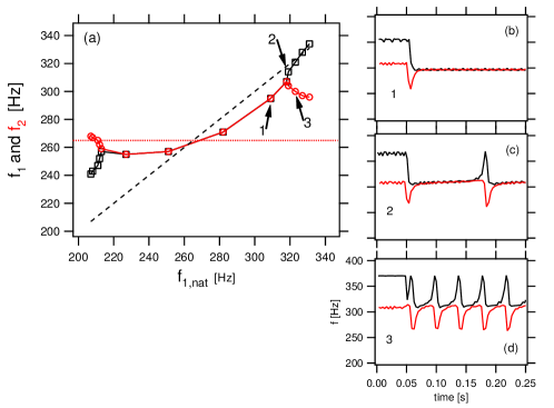
Figure 3: (Color online) (a) Average oscillator frequencies as we vary one of the oscillators’ natural frequencies, indicating the range of frequency mismatch over which two oscillators will still synchronize. These are based on the average period of oscillation over the full $500\,\mbox{ms}$ time series. The dashed black and dotted red lines indicate the self-coupled frequencies of oscillator 1 and 2, respectively; notice that we vary the frequency of the first, but not the second. (b-d) The dynamic frequencies of the two oscillators when coupled, corresponding to points enumerated in (a). The coupling is initially set to zero and then abruptly turned on at $t=0.05\,\mbox{s}$. For (b), the two oscillators quickly come into stable synchronization, but for (c) and (d) this is not the case, as dephasing occurs in bursts. These bursts occur more frequently with larger frequency mismatch.

Figure 3(c) and (d) show how this synchronized state is lost. In (c), we are just beyond the frequency cutoff for synchronization. The two dynamic frequencies initially come together and remain close for many cycles, just like in (b). But then, an abrupt phase slippage occurs (here around $0.18\,\mbox{s}$), at which time the frequency of the faster oscillator momentarily speeds up while the slower oscillator momentarily slows down. During this time the faster oscillator laps the other, and upon catching up their frequencies again match over multiple cycles before the process repeats itself. In (d) the phase breakage occurs more frequently in time. However, even here the frequencies stay intermittently matched over multiple periods of oscillation.

These data present a number of behaviors that are inconsistent with the original Kuramoto model. In Fig. 3(a), the synchronized frequencies exhibit upward curvature; the Kuramoto model predicts linear behavior. At the tail ends of the unsynchronized behavior, the frequencies of the faster oscillators are even faster than their self-coupled frequencies, whereas the Kuramoto model predicts convergence. In (c) and (d), the oscillators’ extreme speeds do not coincide in time, but instead the fast oscillator spikes slightly ahead of the slow oscillator. Upon initial inspection, we expected that a complicated model would be necessary to capture all of these details. Rather than attempt a theoretical derivation of the coupling behavior, we chose instead to find a phenomenological phase oscillator model that explains the system.

To obtain the parameters for our coupling function, we employed an approach similar to that of Kralemann et al. reconstruction , which we describe briefly. Measurements of Wein-bridge oscillators give their voltage. The voltage time series $V\left(t\right)$ must be transformed into a phase time series $\theta\left(t\right)$, called the protophase, by inverting the projection $V\left(t\right)=V_{0}\cos\left(\theta\left(t\right)\right).$ One typically employs the Hilbert transform to obtain the protophase of each oscillator pikovsky-book . If the protophases were taken as the underlying phases, the abrupt phase velocity changes inherent in the behavior of the relaxation oscillators would lead to apparent self-coupling terms. That is, $\dot{\theta}$ depends upon $\theta$. We wish to transform the protophases such that the phase velocity extracted from the uncoupled oscillator data is constant and does not depend upon phase. Therefore, the next step is to obtain a mapping from protophase $\theta\left(t\right)$ to phase $\phi\left(t\right)$. Kralemann suggests obtaining the mapping as $\phi\left(\theta\right)=\omega\int_{0}^{\theta}d\theta^{\prime}\,\sigma\left(\theta^{\prime}\right),$ where $\sigma\left(\theta\right)$ is the probability density of the protophase. We instead obtained the mapping $\theta\to\phi$ directly from the uncoupled time series by assuming that as $\theta$ proceeds from $-\pi$ to $+\pi$ at a variable rate, $\phi$ proceeds from $-\pi$ to $+\pi$ at a constant rate. This set of data forms the basis of a simple interpolation-based mapping that performed as well as the more sophisticated mapping techniques that we tried.

Our next step is to obtain the parameters for a phase oscillator model that adequately describes our results. Knowing that the original Kuramoto model was insufficient, we started by attempting to fit our data to the Sakaguchi-Kuramoto model sakaguchi , which in this case takes the form

$$\dot{\phi}_{i}=\omega_{i}+\frac{K}{N}\sum_{j=1}^{N}\sin\left(\phi_{j}-\phi_{i}-\alpha\right).$$ (1)

Here $\omega_{i}$ represents the uncoupled (angular) frequency of oscillator $i$, which we computed from the average frequency of the uncoupled oscillator time series. We estimated the $\dot{\phi}_{i}$ by performing numerical differentiation on the $\phi_{i}$ time series. To obtain $K$ and $\alpha$, we simultaneously fit the data from both oscillators and across all measurements, obtaining $\alpha=0.509\,\mbox{rad}$ and $K=376\,\mbox{rad/s}$.

Using these best-fit parameters obtained from the extracted phase data, we can now ascertain how well the Sakaguchi-Kuramoto model performs in matching experimental results. For two oscillators, it is fairly straightforward to derive a prediction for the synchronization frequency as a function of mismatch in self-coupled frequency. One thing to remember is that the self-coupled frequency is governed by the case where $N=1$, coming out to $\omega_{i,self}=\omega_{i}-K\sin\alpha$, whereas the pair-coupled behavior is governed by the case where $N=2$. Using this relationship and employing various trigonometric identities, the prediction for the mutually entrained frequency is obtained as

$$f_{entrained}= \frac{f_{1,self}+f_{2,self}}{2}+\frac{K\sin\alpha}{4\pi}$$

$$-\frac{K\sin\alpha}{4\pi}\left(\sqrt{1-4\pi^{2}\frac{\left(f_{1,self}-f_{2,self}\right)^{2}}{K^{2}\cos^{2}\alpha}}\right).$$ (2)

When the oscillators do not mutually entrain, it is possible to compute the amount of time for the faster oscillator to lap the slower oscillator, as well as the phase accumulated by each oscillator. Dividing the phase by the time gives the average phase velocity, from which the average unsychronized frequencies can be calculated:

$$f_{coupled\pm}= \frac{f_{1,self}+f_{2,self}}{2}+\frac{K\sin\alpha}{4\pi}$$

$$\pm\frac{K\cos\alpha}{4\pi}\left(\sqrt{4\pi^{2}\frac{\left(f_{1,self}-f_{2,self}\right)^{2}}{K^{2}\cos^{2}\alpha}-1}\right).$$ (3)

The faster oscillator’s average frequency is $f_{coupled+}$, while the slower oscillator’s average frequency is $f_{coupled-}$. This prediction matches the experimental data extremely closely, as shown in Fig. 4(a). The figure superimposes the analytical result of Eqs. (2) and (3) on the data already presented in Fig. 3. We reiterate that the solid line is not a direct fit to the frequency data points, but the theoretical prediction of the model for our given $\alpha$ and $K$.

The Sakaguchi-Kuramoto model accurately predicts the regime over which the two Wien-bridge oscillators synchronize. The bifurcation occurs at the boundary between Eqs. (2) and (3), which is $\left|f_{1,self}-f_{2,self}\right|=K\,\cos\alpha/\left(2\,\pi\right)$. For our parameters, this condition translates into a predicted maximum self-coupled frequency of $f_{1,self}=319\,\mbox{Hz}$, and a minimum frequency of $214\,\mbox{Hz}$. Inspection of Fig. 4 for these cutoffs reveals excellent agreement with experimental data.

Other features, such as the curvature and asymptotic frequencies, are also correctly predicted. The entrained frequency is predicted to have concave-up curvature. Indeed, just above the the lower-frequency bifurcation point, the mutually entrained frequency drops with increasing $f_{1,self}$, a counterintuitive feature seen in both the prediction and the data. The frequencies at the tail-ends of the measurements can be approximated by assuming that the $-1$ term in Eq. (3) is negligible, leading to an approximation $f_{coupled+}\approx f_{self}+K\sin\alpha/\left(4\pi\right)$; since $\alpha$ is positive, the pair-coupled unsynchronized frequencies far from the entrainment bifurcation will be larger than the self-coupled frequencies.

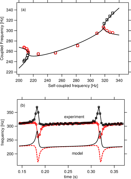
Figure 4: (Color online) (a) A comparison between the theoretical prediction of the Sakaguchi-Kuramoto model, Eqs.(2) and (3), for the 2-oscillator synchronization-frequency (solid line) and the experimental data points shown previously (black squares and red circles, explained in Fig. 3). Good quantitative agreement is found across the whole set of experiments. (b) Just above the highest phase-locked frequency, rapid phase-slippage events at regular time intervals were observed in the experiment: black squares and red circles with connecting lines represent the measured dynamic frequencies of the faster and slower oscillator, respectively. The phenomenon is faithfully reproduced in simulations of the Sakaguchi-Kuramoto model, for which the black solid line and red dashed line represent the faster and slower oscillator, respectively. (In the graph, the trace obtained by numerical simulation is shifted lower for visual clarity.)

As we have seen, above the maximum phase-locked frequency the two oscillators stay in phase with one another for most of the time, but regular phase-slippage events now occur. The time separation of these events decreases with larger oscillator frequency difference. This phenomenon can be reproduced in simulations of the Sakaguchi-Kuramoto model, as depicted in Fig. 4(b). In particular, in both the experimental data and the numerical simulations, we observe the oscillator with the larger self-coupled frequency to break away from the common frequency first, followed in short order by the lower-frequency oscillator. Notice that the simulations also capture the time duration of the phase-slippage events as well as the magnitude of deviation from the common frequency in both directions. This detailed agreement further demonstrates the direct applicability of the Sakaguchi-Kuramoto model to this experimental system of electrical oscillators.

The quantitative accuracy of the Sakaguchi-Kuramoto model is surprising in part because the model is inconsistent with some of the data that we have not presented here. In particular, the phase time series obtained from the self-coupled data can be used to obtain phase velocity as a function of phase, and these phase velocities clearly show a phase dependence. Theorists and modelers often assume that the coupling function can be written as $\Gamma\left(\phi_{j}-\phi_{i}\right)$; Miyazaki and Kinoshita present a concise explanation for why this should be bz-reactors . However, any such model (the Sakaguchi-Kuramoto model being among them) would predict that the self-coupled speeds are related to the uncoupled speeds by a constant offset. They are unable to explain any phase dependence. Fortunately, it appears that these discrepancies are only minor matters.

Our Wien-bridge oscillators were specified to operate in a regime that is characterized by a relaxation oscillator. The dynamics of the protophases seem complicated and aspects of the coupled behavior seemed counter-intuitive. In spite of these complexities, the underlying phase dynamics are surprisingly simple, and can be characterized by the simple and well-studied Sakaguchi-Kuramoto model. Next, we turn our attention to collective behavior that arises simply by altering the coupling topology of an ensemble of such oscillators.

IV Ensemble Measurements

The asymmetries found in the pairwise data have implications for the coupled behavior of larger collections of oscillators. To explore these implications, we prepared a set of 19 oscillators, initially coupled together in an all-to-all network. The self-coupled frequencies of the ensemble were roughly evenly spaced over a frequency range of $\Delta f_{self}=75\,\mbox{Hz}$. In this section we explore the asymmetries, which become even more striking when we consider an all-to-some network.

We begin by systematically examining the fully coupled configuration over a range of coupling values. Figure 5(a) reports the average dynamic frequency of all oscillators for three different values of coupling for this configuration. Series A is for the strongest coupling at $R_{B}=4\,\mbox{k$\Omega$}$ while Series C is for the weakest coupling at $R_{B}=2.5\,\mbox{k$\Omega$}$. Full synchronization could be achieved with a narrower frequency range $\Delta f_{self}$, a stronger coupling, or (as we will show) an altered coupling topology. We chose this combination to highlight an asymmetry in the synchronization that arises for positive $\alpha$: as coupling decreases, the slowest oscillators remain intact while the faster oscillators fall out of synchronization.

Due to this observed asymmetry, we hypothesized that we could increase the degree of synchrony by silencing the slowest oscillators. By opening the $S_{2}$ for some of the slowest oscillators, the equation describing the dynamics changes in a simple but important way. The original Sakaguchi-Kuramoto model includes a self-coupling term, made evident by pulling it out of the all-to-all sum:

$$\dot{\phi}_{i}=\omega_{i}-\frac{K\sin\alpha}{N}+\frac{K}{N}\sum_{j\neq i}\sin\left(\phi_{j}-\phi_{i}-\alpha\right).$$ (4)

Opening $S_{2}$ effectively removes this self-coupling term for the oscillator; from the standpoint of the oscillator just removed, we have essentially increased its natural frequency by an amount $K\sin\alpha/N$. From the standpoint of the other oscillators, the coupling has gotten stronger, going from $K/N$ to $K/\left(N-1\right)$, and the width of the population has gotten narrower because the lower end of the flat spectrum has risen. Also, the self-coupled frequencies of the oscillators at the higher end should be lower (due to higher self-coupling) and the average velocity of the cluster should be closer to the high end of the spectrum. Assuming that the oscillators are indexed in order of increasing frequency and we have silenced the first $n$ of them, we have

$$\dot{\phi}_{i}=\omega_{i}+\frac{K}{N-n}\sum_{j=n+1}^{N}\sin\left(\phi_{j}-\phi_{i}-\alpha\right).$$ (5)

Thus the oscillators that are still “talking” should be more tightly bound than they would have been with the other oscillator present, while the just-removed oscillator will have a higher natural frequency and be interacting with a stronger cluster. Silencing the slowest oscillators should increase synchrony.

Figure 5(b) reports a systematic test of this hypothesis. There are N=19 oscillators altogether, and the horizontal axis records how many of them are talking, i.e. $N-n$ (again, all are listening). The vertical axis marks the value of $R_{B}$. Thus, Fig. 5(b) yields the behavior within accessible parameter space. The color indicates the size of the largest cluster. Not surprisingly, as the coupling is weakened, the synchronized state deteriorates. Full sync is achieved for this system when the coupling is sufficiently strong and/or enough of the slow oscillators have been silenced. Only toward the very right of the figure do we start to lose the slower oscillators.

The figure also depicts the analytically predicted threshold for full synchronization (line and filled circles). Here we first computed, based on the Sakaguchi-Kuramoto model, the value of K at which all the talkers fully synchronized, as well as the associated magnitudes of the mean field $r$ and the coupled frequency $\Omega$. Then, in a second step, it was determined if the non-talkers would be able to entrain to that frequency for a driving signal with magnitude $r\cdot K$. If not, we used an iterative approach to identify the minimum coupling strength at which all oscillators synchronized. The iterative step was only necessary for $N-n\leq 11$ and gives rise to the turning point in the predictions. We see that the computed curve loosely follows the experimental phase boundary.

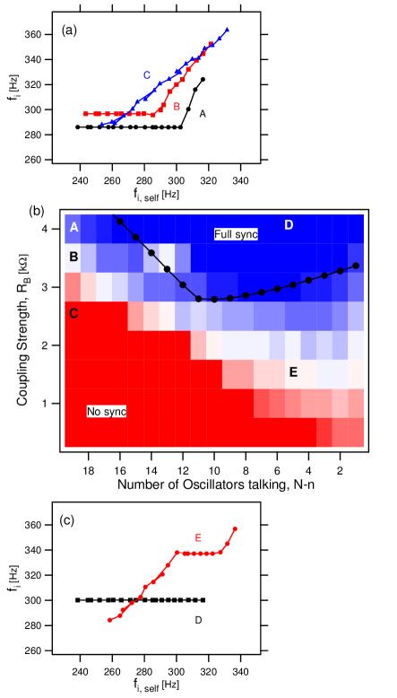
Figure 5: (Color online) (a) Plot of long-time average dynamic frequencies vs self-coupled frequencies for three coupling strengths. The strength decreases from A to C, as indicated by y-value of the same letter in the next figure. (b) The y-axis represents the coupling strength between oscillators as given by the value of $R_{B}$. The x-axis indicates the number of talkers. As we move from left the right, incrementally more low-frequency oscillators are silenced (by opening switch $S_{2}$). The color indicates the size of the largest cluster, ranging from 0 (red, no sync) to 19 (blue, full sync). The line and dots indicates the theoretically predicted threshold for full synchronization. (c) Plot similar to (a) for only five talkers. As with (a), the strength is indicated by the y-value of the same letter in figure (b).

The series presented in 5(a) and 5(c) correspond to the letters in Fig. 5(b). These series provide a detailed snapshot of the behavior at different locations in parameter space. When all oscillators are talking, we see that we lose oscillators from the high-frequency side of the distribution exclusively, until synchronization is completely destroyed. When only the five top oscillators remain as talkers, shown in series D and E, global sync is achieved at the largest coupling strengths, and as the coupling is weakened the cluster loses oscillators on both sides of the distribution.

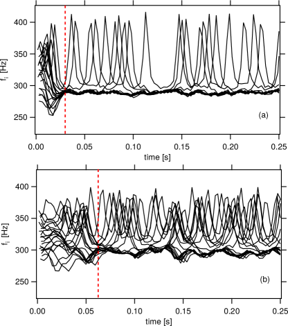
Figure 6: (Color online) Capturing the transients on route to synchronization. Switches, $S_{1}$ and $S_{2}$, are closed for all oscillators. (a) Full coupling strength ($R_{B}=4\,\mbox{k$\Omega$}$) and (b) Reduced coupling strength ($R_{B}=3.5\,\mbox{k$\Omega$}$). The dashed red line marks the approximate end of the transient and the full formation of the synchronized cluster.

Finally we turn to an experimental examination of the route towards synchronization in this system. For this purpose, we capture the initial transients before the steady state establishes itself. In Fig. 6, the dynamic frequency of each oscillator is displayed as a function of time, where t=0 marks the time when the coupling is first turned on. (Before t=0, the oscillators are allowed to free-run.) Here all switches are closed and N=20. In Fig. 6(a), $R_{B}=4\,\mbox{k$\Omega$}$ and in (b) $R_{B}=3.5\,\mbox{k$\Omega$}$.

For the larger coupling strength, we observe that all but the fastest oscillators manage to come in sync within a time of $\Delta t=0.03\,\mbox{s}$. At $300\,\mbox{Hz}$, this corresponds to about 10 periods of oscillation. When the coupling strength is lowered (Fig. 6(b)), the transients last for a longer time, $\Delta t\cong 0.06\,\mbox{s}$, before the synchronized cluster has fully formed.

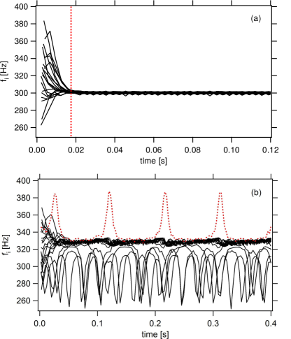
Figure 7: (Color online) Transients for the case where the switches S2 are open for all but the top six oscillators. (a) Full coupling strength ($R_{B}=4\,\mbox{k$\Omega$}$) and (b) Reduced coupling strength ($R_{B}=1.5\,\mbox{k$\Omega$}$). Notice the oscillator with the highest natural frequency (depicted in the dotted red line) experiences periodic bursts in frequency, corresponding to times when its phase detaches from that of the cluster. A few lower-frequency oscillators form a desynchronized random background.

To illustrate the full range of dynamic behavior, it is instructive to repeat this experiment for a point further to the right in parameter space. For this purpose, we open switch $S_{2}$ for all but the fastest six oscillators and consider two values of the coupling. Figure 7 depicts the results. At the largest coupling, Fig. 7(a) clearly indicates global synchronization. In fact, all the oscillators have been entrained within a time of $\Delta t<0.02\,\mbox{s}$, or just a few periods. When the coupling is substantially lowered, a number of interesting behaviors are observed, shown in see Fig. 7(b). Here again the cluster is quickly formed, but we can clearly distinguish the two kinds of unsynchronized behavior. One is a set of “silenced” oscillators, with lower frequencies, and the other is the top oscillator which is also unable to follow the synchronized cluster. Both types of unsynchronized oscillator exhibit the characteristic spike in dynamic frequency indicating a rapid phase-slip event. However, the cluster only responds, to the phase slip event of the faster, talking oscillator. This is evident by the small dip in cluster frequency that slightly lags the frequency spike of the fast oscillator. This lead/lag behavior was also seen in the pairwise interactions (Fig. 3). The magnitude of the change differs, reflecting a single oscillator interacting with a cluster of many oscillators, in agreement with the Sakaguchi-Kuramoto model.

V Conclusion

In this work, we have studied a network of simple Wien-bridge oscillators in an experimental regime for which they can be approximated as phase oscillators. Using the experimental data for a pair of oscillators, we determined the two adjustable parameters within the Sakaguchi-Kuramoto model. We then tested detailed, quantitative predictions of this model against experimental findings. Such a comparison yielded surprisingly good agreement.

As an additional illustration of the effectiveness of the model, we introduced and experimentally measured the behavior of a new kind of coupling, termed all-to-some, in which all oscillators are coupled to a signal that is constructed from only some of the oscillators. For positive $\alpha$, we demonstrated that selective removal of the slowest oscillators can improve the degree of global synchronization, an observation that is consistent with the Sakaguchi-Kuramoto model. The experimental data clearly shows the evolution towards collective synchronization in this system when the coupling is turned on. It also illustrates the way synchronization is lost when the coupling is incrementally weakened.

These oscillators are ideal for synchronization experiments. They are easy to build. As we have illustrated, the underlying phase dynamics are well described by a simple model commonly studied in the synchronization literature. The topology and nature of the interactions can be easily prescribed. Nearly every aspect of the system can be easily measured. In a field where numerical simulations are the norm, we believe that a collection of electronic oscillators built using this design can serve as a general-purpose system for real experimental tests of the theories of synchronization.

References

- (1) J. Buck and E. Buck, Sci. Am. 234, 7485 (1976).
- (2) T. J. Walker, Science 166, 891 (1969).
- (3) I. Z. Kiss, Y. Zhai, and J. L. Hudson, Phys. Rev. E 77, 046204 (2008).
- (4) H. Fukuda, N. Tamari, H. Morimura, and S. Kai, J. Phys. Chem. A 109, 11250 (2005).
- (5) M.S. Paoletti, C. R. Nugent, and T. H. Solomon, Phys. Rev. Lett. 96, 124101 (2006).
- (6) S. Strogatz, D. Abrams, A. McRobie, B. Eckhardt, and E. Ott, Nature 438, 43 (2005).
- (7) D. Mertens and R. Weaver, Phys. Rev. E 83, 046221 (2011).
- (8) M. Zhang, G. S. Wiederhecker, S. Manipatruni, A. Barnard, P. McEuen, and M. Lipson, Phys. Rev. Lett. 109, 233906 (2012).
- (9) D. Michaels, E. Matyas, and J. Jalife, Circulation Res. 61, 704 (1987).
- (10) H. Sompolinsky, D. Golomb, and D. Kleinfeld, Phys. Rev. A 43, 6990 (1991).
- (11) M. Breakspear, S. Heitmann and A. Daffertshofer, Front. Hum. Neurosci. 4, 190 (2010).
- (12) Kuramoto, Y., Chemical Oscillations, Waves and Turbulence. 1984, (Berlin: Springer Verlag).
- (13) H. Sakaguchi and Y. Kuramoto, Prog. Theor. Phys. 76, 576 (1986).
- (14) Y. Kuramoto and I. Nishikawa, J. Stat. Phys., 49, 569 (1987).
- (15) S. H. Strogatz, Physica D 143, 1 (2000).
- (16) A. Pikovsky, M. Rosenblum, J. Kurths, Synchronization: A Universal Concept in Nonlinear Sciences. 2003 (Cambridge university press).
- (17) E. Ott T. M. Antonsen. Chaos 18, 037113 (2008).
- (18) S. Yu. Kourtchatov, V. V. Likhanskii, A. P. Napartovich, F. T. Arecchi, A. Lapucci, Phys. Rev. A 52, 4089 (1995).
- (19) K. Wiesenfeld, P. Colet, S. H. Strogatz, Phys. Rev. Lett. 76, 404 (1996).
- (20) J. Miyazaki, S. Kinoshita. Physical Review Letters 96, 194101 (2006).
- (21) J. Delgado, N. Li, M. Leda, H. O. Gonzalez-Ochoa, S. Fraden, I. R. Epstein. Soft Matter 7, 3155-67 (2011).
- (22) A. Bergner, M. Frasca, G. Sciuto, A. Buscarino, E. J. Ngamga, L. Fortuna, and J. Kurths. Physical Review E 85, (2012): 026208.
- (23) L. V. Gambuzza, A. Buscarino, S. Chessari, L. Fortuna, R. Meucci, M. Frasca. Physical Review E 90, (2014): 032905.
- (24) A. A. Temirbayev, Z. Z. Zhanabaev, S. B. Tarasov, V. I. Ponomarenko, M. Rosenblum, Phys. Rev. E 85, 015204 (2012).
- (25) S. Moro, Y. Nishio, and S. Mori, IEICE Trans. Fundamentals E78-A, 244 (1995).
- (26) T. E. Lee, G. Refael, M. C. Cross, O. Kogan, J. L. Rogers. Physical Review E 80, 046210 (2009).
- (27) D. M. Abrams, S. H. Strogatz. International Journal of Bifurcation and Chaos 16, 21 (2006).
- (28) B. Kralemann, A. Pikovsky, M. Rosenblum. Chaos 21, 025104 (2011).
- (29) B. Kralemann, L. Cimponeriu, M. Rosenblum, A. Pikovsky, R. Mrowka. Physical Review E 77, 066205 (2008).