Robust A Posteriori Error Estimation for Finite Element Approximation to $\bm{H}(\mathbf{curl})$ Problem

Abstract

In this paper, we introduce a novel a posteriori error estimator for the conforming finite element approximation to the $\bm{H}(\mathbf{curl}\hskip 0.7pt)$ problem with inhomogeneous media and with the right-hand side only in $\bm{L}^{2}$. The estimator is of the recovery type. Independent with the current approximation to the primary variable (the electric field), an auxiliary variable (the magnetizing field) is recovered in parallel by solving a similar $\bm{H}(\mathbf{curl}\hskip 0.7pt)$ problem. An alternate way of recovery is presented as well by localizing the error flux. The estimator is then defined as the sum of the modified element residual and the residual of the constitutive equation defining the auxiliary variable. It is proved that the estimator is approximately equal to the true error in the energy norm without the quasi-monotonicity assumption. Finally, we present numerical results for several $\bm{H}(\mathbf{curl}\hskip 0.7pt)$ interface problems.

1 Introduction

Let $\Omega$ be a bounded and simply-connected polyhedral domain in $\mathbb{R}^{3}$ with boundary $\partial\Omega=\bar{\Gamma}_{D}\cup\bar{\Gamma}_{N}$ and $\Gamma_{D}\cap\Gamma_{N}=\emptyset$, and let $\bm{n}=(n_{1},n_{2},n_{3})$ be the outward unit vector normal to the boundary. Denote by $\bm{u}$ the electric field, we consider the following $\bm{H}(\mathbf{curl}\hskip 0.7pt)$ model problem originated from a second order hyperbolic equation by eliminating the magnetic field in Maxwell’s equations:

$$\left\{\begin{array}[]{rcll}\nabla\!\times\!(\mu^{-1}\nabla\!\times\!\bm{u})+\beta\,\bm{u}&=&\bm{f},&\;\text{ in }\,\Omega,\\[5.69054pt] \bm{u}\!\times\!\bm{n}&=&\bm{g}_{{}_{D}},&\;\text{ on }\,\Gamma_{D},\\[5.69054pt] (\mu^{-1}\nabla\!\times\!\bm{u})\!\times\!\bm{n}&=&\bm{g}_{{}_{N}},&\;\text{ on }\,\Gamma_{N},\end{array}\right.$$ (1.1)

where $\nabla\!\times\!$ is the curl operator; the $\bm{f}$, $\bm{g}_{{}_{D}}$, and $\bm{g}_{{}_{N}}$ are given vector fields which are assumed to be well-defined on $\Omega$, $\Gamma_{D}$, and $\Gamma_{N}$, respectively; the $\mu$ is the magnetic permeability; and the $\beta$ depends on the electrical conductivity, the dielectric constant, and the time step size. Assume that the coefficients $\mu^{-1}\in\bm{L}^{\infty}(\Omega)$ and $\beta\in\bm{L}^{\infty}(\Omega)$ are bounded below

$$0<\mu_{0}^{-1}\leq\mu^{-1}(\bm{x})\quad\mbox{and}\quad 0<\beta_{0}\leq\beta(\bm{x})$$

for almost all $\bm{x}\in\Omega$.

The a posteriori error estimation for the conforming finite element approximation to the $\bm{H}(\mathbf{curl}\hskip 0.7pt)$ problem in (1.1) has been studied recently by several researchers. Several types of a posteriori error estimators have been introduced and analyzed. These include residual-based estimators and the corresponding convergence analysis (explicit [3, 10, 11, 12, 27, 29, 34], and implicit [18]), equilibrated estimators [4], and recovery-based estimators [6, 28]. There are four types of errors in the explicit residual-based estimator (see [3]). Two of them are standard, i.e., the element residual, and the interelement face jump induced by the discrepancy induced by integration by parts associated with the original equation in (1.1). The other two are also the element residual and the interelement face jump, but associated with the divergence of the original equation: $\nabla\!\cdot\!(\beta\bm{u})=\nabla\!\cdot\!\bm{f}$, where $\nabla\!\cdot\!$ is the divergence operator. These two quantities measure how good the approximation is in the kernel space of the curl operator.

Recently, the idea of the robust recovery estimator explored in [7, 8] for the diffusion interface problem has been extended to the $\bm{H}(\mathbf{curl}\hskip 0.7pt)$ interface problem in [6]. Instead of recovering two quantities in the continuous polynomial spaces like the extension of the popular Zienkiewicz-Zhu (ZZ) error estimator in [28], two quantities related to $\mu^{-1}\nabla\!\times\!\bm{u}$ and $\beta\bm{u}$ are recovered in the respective $\bm{H}(\mathbf{curl}\hskip 0.7pt)$- and $\bm{H}(\operatorname{div})$-conforming finite element spaces. The resulting estimator consists of four terms similar to the residual estimator in the pioneering work [3] on this topic by Beck, Hiptmair, Hoppe, and Wohlmuth: two of them measure the face jumps of the tangential components and the normal component of the numerical approximations to $\mu^{-1}\nabla\!\times\!\bm{u}$ and $\beta\bm{u}$, respectively, and the other two are element residuals of the recovery type.

All existing a posteriori error estimators for the $\bm{H}(\mathbf{curl}\hskip 0.7pt)$ problem assume that the right-hand side $\bm{f}$ is in $\bm{H}(\operatorname{div})$ or divergence free. This assumption does not hold in many applications (e.g. the implicit marching scheme mentioned in [19]). Moreover, two terms of the estimators are associated with the divergence of the original equation. In the proof, these two terms come to existence up after performing the integration by parts for the irrotational gradient part of the error, which lies in the kernel of the curl operator. One of the key technical tools, a Helmholtz decomposition, used in this proving mechanism, relies on $\bm{f}$ being in $\bm{H}(\operatorname{div})$, and fails if $\bm{f}\notin\bm{H}(\operatorname{div})$. In [12], the assumption that $\bm{f}\in\bm{H}(\operatorname{div})$ is weakened to $\bm{f}$ being in the piecewise $\bm{H}(\operatorname{div})$ space with respect to the triangulation, at the same time, the divergence residual and norm jump are modified to incorporate this relaxation. Another drawback of using Helmholtz decomposition on the error is that it introduces the assumption of the coefficients’ quasi-monotonicity into the proof pipeline. An interpolant with a coefficient independent stability bound is impossible to construct in a “checkerboard” scenario (see [32] for diffusion case, and [6] for $\bm{H}(\mathbf{curl}\hskip 0.7pt)$ case). To gain certain robustness for the error estimator in the proof, one has to assume the coefficients distribution is quasi-monotone. However, in an earlier work of Chen, Xu, and Zou ([11]), it is shown that numerically this quasi-monotonicy assumption is more of an artifact introduced by the proof pipeline, at least for the irrotational vector fields. As a result, we conjecture that the divergence related terms should not be part of an estimator if it is appropriately constructed. In Section 5, some numerical justifications are presented to show the unnecessity of including the divergence related terms.

The pioneering work in using the dual problems for a posteriori error estimation dates back to [30]. In [30], Oden, Demkowicz, Rachowicz, and Westermann studied the a posteriori error estimation through duality for the diffusion-reaction problem. The finite element approximation to a dual problem is used to estimate the error for the original primal problem (diffusion-reaction). The result shares the same form to the Prague-Synge identity ([33]) for diffusion-reaction problem. The method presented in this paper may be viewed as an extension of the duality method in [30] to the $\bm{H}(\mathbf{curl}\hskip 0.7pt)$ interface problem. The auxiliary magnetizing field introduced in Section 3 is the dual variable resembling the flux variable in [30]. The connection is illustrated in details in Section 4.1.

Later, Repin ([31]) proposes a functional type a posteriori error estimator of $\bm{H}(\mathbf{curl}\hskip 0.7pt)$ problem, which can be viewed as an extension of the general approach in [30]. Repin et al ([26]) improve the estimate by assuming that the data $\bm{f}$ is divergence free and the finite element approximation is in $\bm{H}(\operatorname{div})$. In [31], the upper bound is established through integration by parts by introducing an auxiliary variable in an integral identity for $\bm{H}(\mathbf{curl}\hskip 0.7pt)$. An auxiliary variable is recovered by globally solving an $\bm{H}(\mathbf{curl}\hskip 0.7pt)$ finite element approximation problem and is used in the error estimator. For the global lower bound, the error equation is solved globally in an $\bm{H}(\mathbf{curl}\hskip 0.7pt)$ conforming finite element space. Then the solution is inserted into the functional as the error estimator of which the maximizer corresponds to the solution to the error equation.

The purpose of this paper is to develop a novel a posteriori error estimator for the conforming finite element approximation to the $\bm{H}(\mathbf{curl}\hskip 0.7pt)$ problem in (2.1) that overcomes the above drawbacks of the existing estimators, e.g. the Helmholtz decomposition proof mechanism, restricted by the assumption that $\bm{f}\in\bm{H}(\operatorname{div};\Omega)$ or divergence free, which brings in the divergence related terms. Specifically, the estimator studied in this paper is of the recovery type, requires the right-hand side merely having a regularity of $\bm{L}^{2}$, and has only two terms that measure the element residual and the tangential face jump of the original equation. Based on the current approximation to the primary variable $\bm{u}$ (the electric field), an auxiliary variable $\bm{\sigma}$ (the magnetizing field) is recovered by approximating a similar auxiliary $\bm{H}(\mathbf{curl}\hskip 0.7pt)$ problem. To this end, a multigrid smoother is used to approximate this auxiliary problem, which is independent of the primary equation and is performed in parallel with the primary problem. The cost is the same order of complexity with computing the residual-based estimator, which is much less than solving the original $\bm{H}(\mathbf{curl}\hskip 0.7pt)$ problem.

An alternate route is illustrated as well in Section 3.2 by approximating a localized auxiliary problem. While embracing the locality, the parallel nature using the multigrid smoother is gone. The recovery through approximating localized problem requires the user to provide element residual and tangential face jump of the numerical magnetizing field based on the finite element solution of the primary equation. The estimator is then defined as the sum of the modified element residual and the residual of the auxiliary constitutive equation. It is proved that the estimator is equal to the true error in the energy norm globally. Moreover, in contrast to the mechanism of the proof using Helmholtz decomposition mentioned previously, the decomposition is avoided by using the joint energy norm. As a result, the new estimator’s reliability does not rely on the coefficients distribution (Theorem 4.2).

Meanwhile, in this paper, the method and analysis extend the functional-type error estimator in [31] to a more pragmatic context by including the mixed boundary conditions, and furthermore, the auxiliary variable $\bm{\sigma}$ is approximated by a fast multigrid smoother, or by solving a localized $\bm{H}(\mathbf{curl}\hskip 0.7pt)$ problem on vertex patches, to avoid solving a global finite element approximation problem.

Lastly, in order to compare the new estimator introduced in this paper with existing estimators, we present numerical results for $\bm{H}(\mathbf{curl}\hskip 0.7pt)$ intersecting interface problems. When $\bm{f}\notin\bm{H}(\operatorname{div})$, the mesh generated by our indicator is much more efficient than those by existing indicators (Section 5).

2 Primal Problem and The Finite Element Approximation

Denote by $\bm{L}^{2}(\Omega)$ the space of the square integrable vector fields in $\mathbb{R}^{3}$ equipped with the standard $\bm{L}^{2}$ norm: $\left\|{\bm{v}}\right\|_{\omega}=\sqrt{(\bm{v},\,\bm{v})_{\omega}}$, where $(\bm{u},\,\bm{v})_{\omega}:=\displaystyle\int_{\omega}\bm{u}\cdot\bm{v}\,d\bm{x}$ denotes the standard $\bm{L}^{2}$ inner product over an open subset $\omega\subseteq\Omega$, when $\omega=\Omega$, the subscript is dropped for $\left\|{\bm{v}}\right\|:=\left\|{\bm{v}}\right\|_{\Omega}$ and $(\bm{u},\,\bm{v})=(\bm{u},\,\bm{v})_{\Omega}$. Let

$$\bm{H}(\mathbf{curl}\hskip 0.7pt;\Omega):=\{\bm{v}\in\bm{L}^{2}(\Omega):\nabla\!\times\!\bm{v}\in\bm{L}^{2}(\Omega)\},$$

which is a Hilbert space equipped with the norm

$$\left\|{\bm{v}}\right\|_{\bm{H}(\mathbf{curl}\hskip 0.7pt)}=\Bigl{(}\left\|{\bm{v}}\right\|^{2}+\left\|{\nabla\!\times\!\bm{v}}\right\|^{2}\Bigr{)}^{1/2}.$$

Denote its subspaces by

$$\begin{array}[]{l}\bm{H}_{B}(\mathbf{curl}\hskip 0.7pt;\Omega):=\{\bm{v}\in\bm{H}(\mathbf{curl}\hskip 0.7pt;\Omega):\bm{v}\!\times\!\bm{n}=\bm{g}_{{}_{B}}\text{ on }\Gamma_{B}\}\\[5.69054pt] \mbox{and}\quad{\mathop{{}\bm{H}}\limits^{\vbox to-0.3014pt{\kern-1.50694pt\hbox{$\scriptstyle\circ$}\vss}}}_{B}(\mathbf{curl}\hskip 0.7pt;\Omega):=\{\bm{v}\in\bm{H}_{B}(\mathbf{curl}\hskip 0.7pt;\Omega):\bm{g}_{{}_{B}}={\bf 0}\}\end{array}$$

for $B=D$ or $N$.

For any $\bm{v}\in{\mathop{{}\bm{H}}\limits^{\vbox to-0.3014pt{\kern-1.50694pt\hbox{$\scriptstyle\circ$}\vss}}}_{D}(\mathbf{curl}\hskip 0.7pt;\Omega)$, multiplying the first equation in (1.1) by a suitable test function $\bm{v}$ with vanishing tangential part on $\Gamma_{D}$, integrating over the domain $\Omega$, and using integration by parts formula for $\bm{H}(\mathbf{curl}\hskip 0.7pt)$-regular vector fields (e.g. see [2]), we have

$$(\bm{f},\,\bm{v}) = \big{(}\nabla\!\times\!(\mu^{-1}\nabla\!\times\!\bm{u}),\,\bm{v}\big{)}+(\beta\,\bm{u},\,\bm{v})$$

$$= (\mu^{-1}\nabla\!\times\!\bm{u},\,\nabla\!\times\!\bm{v})+(\beta\,\bm{u},\,\bm{v})-\int_{\Gamma_{N}}\bm{g}_{{}_{N}}\cdot\bm{v}\,dS.$$

Then the weak form associated to problem (1.1) is to find $\bm{u}\in\bm{H}_{D}(\mathbf{curl}\hskip 0.7pt;\Omega)$ such that

$$A_{\mu,\beta}(\bm{u},\bm{v})=f_{{}_{N}}(\bm{v}),\quad\forall\;\bm{v}\in{\mathop{{}\bm{H}}\limits^{\vbox to-0.3014pt{\kern-1.50694pt\hbox{$\scriptstyle\circ$}\vss}}}_{D}(\mathbf{curl}\hskip 0.7pt;\Omega),$$ (2.1)

where the bilinear and linear forms are given by

$$\begin{gathered}A_{\mu,\beta}(\bm{u},\bm{v})=(\mu^{-1}\nabla\!\times\!\bm{u},\nabla\!\times\!\bm{v})+(\beta\,\bm{u},\bm{v})\quad\mbox{and}\quad f_{{}_{N}}(\bm{v})=(\bm{f},\bm{v})+{\left\langle{\bm{g}_{{}_{N}}},{\bm{v}}\right\rangle}_{\Gamma_{N}},\end{gathered}$$

respectively. Here, ${\left\langle{\bm{g}_{{}_{N}}},{\bm{v}}\right\rangle}_{\Gamma_{N}}=\displaystyle\int_{\Gamma_{N}}\bm{g}_{{}_{N}}\cdot\bm{v}\,dS$ denotes the duality pair over $\Gamma_{N}$. Denote by

$$\mathopen{|\mkern-2.5mu|\mkern-2.5mu|}\bm{v}\mathclose{|\mkern-2.5mu|\mkern-2.5mu|}_{\mu,\beta}=\sqrt{A_{\mu,\beta}(\bm{v},\bm{v})}$$

the “energy” norm induced by the bilinear form $A_{\mu,\beta}(\cdot,\,\cdot)$.

Theorem 2.1.

Assume that $\bm{f}\in\bm{L}^{2}(\Omega)$, $\bm{g}_{{}_{D}}\in\bm{X}_{\mathop{\mathchoice{\textstyle\mathbin{\!/\mkern-5.0mu/\!}}{\scriptstyle\mathbin{\!/\mkern-5.0mu/\!}}{\scriptscriptstyle\mathbin{\!/\mkern-5.0mu/\!}}{\scriptscriptstyle\mathbin{\!/\mkern-5.0mu/\!}}}\nolimits}(\Gamma_{D})$, and $\bm{g}_{{}_{N}}\in\bm{H}^{1/2}_{\perp}(\Gamma_{N})$. Then the weak formulation of (1.1) has a unique solution $\bm{u}\in\bm{H}_{D}(\mathbf{curl}\hskip 0.7pt;\Omega)$ satisfying the following a priori estimate

$$\mathopen{|\mkern-2.5mu|\mkern-2.5mu|}\bm{u}\mathclose{|\mkern-2.5mu|\mkern-2.5mu|}_{\mu,\beta}\leq\|{\beta^{-1/2}\bm{f}}\|+\left\|{\bm{g}_{{}_{D}}}\right\|_{-1/2,\mu,\beta,\Gamma_{D}}+\left\|{\bm{g}_{{}_{N}}}\right\|_{1/2,\mu,\beta,\Gamma_{N}}.$$ (2.2)

Proof.

For the notations and proof, see the Appendix A. ∎

2.1 Finite Element Approximation

For simplicity of the presentation, only the tetrahedral elements are considered. Let ${\mathcal{T}}=\{K\}$ be a finite element partition of the domain $\Omega$. Denote by $h_{K}$ the diameter of the element $K$. Assume that the triangulation ${\mathcal{T}}$ is regular and quasi-uniform.

Let $\bm{P}_{k}(K)=P_{k}(K)^{3}$ where $P_{k}(K)$ is the space of polynomials of degree less than or equal to $k$. Let $\widetilde{P}_{k+1}(K)$ and $\widetilde{\bm{P}}_{k+1}(K)$ be the spaces of homogeneous polynomials of scalar functions and vector fields. Denote by the first or second kind Nédélec elements (e.g. see [24, 25])

$$\bm{{\mathcal{N}}\!{\mathcal{D}}}^{k}=\{\bm{v}\in\bm{H}(\mathbf{curl}\hskip 0.7pt;\Omega):\bm{v}\big{|}_{\raisebox{-0.5pt}{\scriptsize$K$}}\in\bm{{\mathcal{N}}\!{\mathcal{D}}}^{k,i}(K)\,\;\forall\,\,K\in{\mathcal{T}}\}\subset\bm{H}(\mathbf{curl}\hskip 0.7pt;\Omega),$$

for $i=1,\,2$, respectively, where the local Nédélec elements are given by

$$\bm{{\mathcal{N}}\!{\mathcal{D}}}^{k,1}(K)=\{\bm{p}+\bm{s}:\bm{p}\in\bm{P}_{k}(K),\bm{s}\in\widetilde{\bm{P}}_{k+1}(K)\text{ such that }\bm{s}\cdot\bm{x}=0\}$$

and $$\bm{{\mathcal{N}}\!{\mathcal{D}}}^{k,2}(K)=\{\bm{p}+\nabla s:\bm{p}\in\bm{{\mathcal{N}}\!{\mathcal{D}}}^{k,1}(K),s\in\widetilde{P}_{k+2}(K)\}.$$

For simplicity of the presentation, we assume that both boundary data $\bm{g}_{{}_{D}}$ and $\bm{g}_{{}_{N}}$ are piecewise polynomials, and the polynomial extension (see [14]) of the Dirichlet boundary data as the tangential trace is in $\bm{{\mathcal{N}}\!{\mathcal{D}}}^{k}$. Now, the conforming finite element approximation to (1.1) is to find $\bm{u}_{{}_{\mathcal{T}}}\in\bm{{\mathcal{N}}\!{\mathcal{D}}}^{k}\cap{\bm{H}}_{D}(\mathbf{curl}\hskip 0.7pt;\Omega)$ such that

$$A_{\mu,\beta}(\bm{u}_{{}_{\mathcal{T}}},\,\bm{v})=f_{{}_{N}}(\bm{v}),\quad\forall\,\,\bm{v}\in\bm{{\mathcal{N}}\!{\mathcal{D}}}^{k}\cap{\mathop{{}\bm{H}}\limits^{\vbox to-0.3014pt{\kern-1.50694pt\hbox{$\scriptstyle\circ$}\vss}}}_{D}(\mathbf{curl}\hskip 0.7pt;\Omega).$$ (2.3)

Assume that $\bm{u}$ and $\bm{u}_{{}_{\mathcal{T}}}$ are the solutions of the problems in (1.1) and (2.3), respectively, and that $\bm{u}\in\bm{H}^{k+1}(\Omega)$, $\nabla\!\times\!\bm{u}\in\bm{H}^{k+1}(\Omega)$ (When the regularity assumption is not met, one can construct a curl-preserving mollification, see [16]), by the interpolation result from [24] Chapter 5 and Céa’s lemma, one has the following a priori error estimation:

$$\mathopen{|\mkern-2.5mu|\mkern-2.5mu|}\bm{u}-\bm{u}_{{}_{\mathcal{T}}}\mathclose{|\mkern-2.5mu|\mkern-2.5mu|}_{\mu,\beta}\leq C\,h^{k+1}\Big{(}\|\bm{u}\|_{{}_{\bm{H}^{k+1}(\Omega)}}+\|\nabla\!\times\!\bm{u}\|_{{}_{\bm{H}^{k+1}(\Omega)}}\Big{)},$$ (2.4)

where $C$ is a positive constant independent of the mesh size $h=\max\limits_{K\in{\mathcal{T}}}h_{K}$.

3 Auxiliary Problem of Magnetizing Field

3.1 Recovery of the magnetizing field

Introducing the magnetizing field

$$\bm{\sigma}=\mu^{-1}\nabla\!\times\!\bm{u},$$ (3.1)

then the first equation in (1.1) becomes

$$\nabla\!\times\!\bm{\sigma}+\beta\,\bm{u}=\bm{f},\;\mbox{ in }\,\Omega.$$ (3.2)

The boundary condition on $\Gamma_{N}$ may be rewritten as follows

$$\bm{\sigma}\!\times\!\bm{n}=\bm{g}_{{}_{N}},\;\text{ on }\,\Gamma_{N}.$$

For any $\bm{\tau}\in{\mathop{{}\bm{H}}\limits^{\vbox to-0.3014pt{\kern-1.50694pt\hbox{$\scriptstyle\circ$}\vss}}}_{N}(\mathbf{curl}\hskip 0.7pt;\Omega)$, multiplying equation (3.2) by $\beta^{-1}\nabla\!\times\!\bm{\tau}$, integrating over the domain $\Omega$, and using integration by parts and (3.1), we have

$$(\beta^{-1}\bm{f},\,\nabla\!\times\!\bm{\tau}) = (\beta^{-1}\nabla\!\times\!\bm{\sigma},\,\nabla\!\times\!\bm{\tau})+(\bm{u},\,\nabla\!\times\!\bm{\tau})$$

$$= (\beta^{-1}\nabla\!\times\!\bm{\sigma},\,\nabla\!\times\!\bm{\tau})+(\nabla\!\times\!\bm{u},\,\bm{\tau})$$

$$\;+\int_{\Gamma_{D}}(\bm{u}\!\times\!\bm{n})\cdot\bm{\tau}\,ds-\int_{\Gamma_{N}}\bm{u}\cdot(\bm{\tau}\!\times\!\bm{n})\,ds$$

$$= (\beta^{-1}\nabla\!\times\!\bm{\sigma},\,\nabla\!\times\!\bm{\tau})+(\mu\,\bm{\sigma},\,\bm{\tau})+\int_{\Gamma_{D}}\bm{g}_{{}_{D}}\cdot\bm{\tau}\,ds.$$

Hence, the variational formulation for the magnetizing field is to find $\bm{\sigma}\in\bm{H}_{N}(\mathbf{curl}\hskip 0.7pt;\Omega)$ such that

$$A_{\beta,\mu}(\bm{\sigma},\bm{\tau})=f_{{}_{D}}(\bm{\tau}),\quad\forall\;\bm{\tau}\in{\mathop{{}\bm{H}}\limits^{\vbox to-0.3014pt{\kern-1.50694pt\hbox{$\scriptstyle\circ$}\vss}}}_{N}(\mathbf{curl}\hskip 0.7pt;\Omega),$$ (3.3)

where the bilinear and linear forms are given by

$$A_{\beta,\mu}(\bm{\sigma},\bm{\tau})=(\beta^{-1}\nabla\!\times\!\bm{\sigma},\nabla\!\times\!\bm{\tau})+(\mu\,\bm{\sigma},\bm{\tau})\quad\mbox{and}\quad f_{{}_{D}}(\bm{\tau})=(\beta^{-1}\bm{f},\nabla\!\times\!\bm{\tau})-{\left\langle{\bm{g}_{{}_{D}}},{\bm{\tau}}\right\rangle}_{\Gamma_{D}},$$

respectively. The natural boundary condition for the primary problem becomes the essential boundary condition for the auxiliary problem, while the essential boundary condition for the primary problem is now incorporated into the right-hand side and becomes the natural boundary condition. Denote the “energy” norm induced by $A_{\beta,\mu}(\cdot,\,\cdot)$ by

$$\mathopen{|\mkern-2.5mu|\mkern-2.5mu|}\bm{\tau}\mathclose{|\mkern-2.5mu|\mkern-2.5mu|}_{\beta,\mu}=\sqrt{A_{\beta,\mu}(\bm{\tau},\bm{\tau})}.$$

Theorem 3.1.

Assume that $\bm{f}\in\bm{L}^{2}(\Omega)$, $\bm{g}_{{}_{D}}\in\bm{H}^{1/2}_{\perp}(\Gamma_{D})$, and $\bm{g}_{{}_{N}}\in\bm{X}_{\mathop{\mathchoice{\textstyle\mathbin{\!/\mkern-5.0mu/\!}}{\scriptstyle\mathbin{\!/\mkern-5.0mu/\!}}{\scriptscriptstyle\mathbin{\!/\mkern-5.0mu/\!}}{\scriptscriptstyle\mathbin{\!/\mkern-5.0mu/\!}}}\nolimits}(\Gamma_{N})$. Then problem (3.3) has a unique solution $\bm{\sigma}\in\bm{H}_{N}(\mathbf{curl}\hskip 0.7pt;\Omega)$ satisfying the following a priori estimate

$$\mathopen{|\mkern-2.5mu|\mkern-2.5mu|}\bm{\sigma}\mathclose{|\mkern-2.5mu|\mkern-2.5mu|}_{\beta,\mu}\leq\|\beta^{-1/2}\bm{f}\|+\left\|{\bm{g}_{{}_{D}}}\right\|_{1/2,\mu,\beta,\Gamma_{D}}+\left\|{\bm{g}_{{}_{N}}}\right\|_{-1/2,\beta,\mu,\Gamma_{N}}.$$ (3.4)

Proof.

The theorem may be proved in a similar fashion as Theorem 2.1. ∎

Similarly to that for the essential boundary condition, it is assumed that the polynomial extension of the Neumman boundary data as the tangential trace is in $\bm{{\mathcal{N}}\!{\mathcal{D}}}^{k}$ as well. Now, the conforming finite element approximation to (3.3) is to find $\bm{\sigma}_{{}_{\mathcal{T}}}\in\bm{{\mathcal{N}}\!{\mathcal{D}}}^{k}\cap\bm{H}_{N}(\mathbf{curl}\hskip 0.7pt;\Omega)$ such that

$$A_{\beta,\mu}(\bm{\sigma}_{{}_{\mathcal{T}}},\,\bm{\tau})=f_{{}_{D}}(\bm{\tau}),\quad\forall\;\bm{\tau}\in\bm{{\mathcal{N}}\!{\mathcal{D}}}^{k}\cap{\mathop{{}\bm{H}}\limits^{\vbox to-0.3014pt{\kern-1.50694pt\hbox{$\scriptstyle\circ$}\vss}}}_{N}(\mathbf{curl}\hskip 0.7pt;\Omega).$$ (3.5)

Assume that $\bm{\sigma}$ and $\bm{\sigma}_{{}_{\mathcal{T}}}$ are the solutions of the problems in (3.1) and (3.5), respectively, and that $\bm{\sigma}\in\bm{H}^{k+1}(\Omega)$, $\nabla\!\times\!\bm{\sigma}\in\bm{H}^{k+1}(\Omega)$, one has the following a priori error estimation similar to (2.4)

$$\mathopen{|\mkern-2.5mu|\mkern-2.5mu|}\bm{\sigma}-\bm{\sigma}_{{}_{\mathcal{T}}}\mathclose{|\mkern-2.5mu|\mkern-2.5mu|}_{\mu,\beta}\leq C\,h^{k+1}\Big{(}\|\bm{\sigma}\|_{{}_{\bm{H}^{k+1}(\Omega)}}+\|\nabla\!\times\!\bm{\sigma}\|_{{}_{\bm{H}^{k+1}(\Omega)}}\Big{)}.$$ (3.6)

The a priori estimate shows that heuristically, for the auxiliary magnetizing field $\bm{\sigma}$, using the same order $\bm{H}(\mathbf{curl}\hskip 0.7pt)$-conforming finite element approximation spaces with the primary variable $\bm{u}$ may be served as the building blocks for the a posteriori error estimation.

3.2 Localization of the recovering procedure

The localization of the recovery of $\bm{\sigma}_{{}_{\mathcal{T}}}$ for this new $\bm{H}(\mathbf{curl}\hskip 0.7pt)$ recovery shares similar methodology with the one used in the equilibrated flux recovery (see [4, 5]). However, due to the presence of the $\bm{L}^{2}$-term, exact equilibration is impossible due to several discrepancies: $\nabla\!\times\!\bm{\sigma}_{{}_{\mathcal{T}}}+\beta\bm{u}_{{}_{\mathcal{T}}}\neq\bm{f}$ if $\bm{\sigma}_{{}_{\mathcal{T}}}$ and $\bm{u}_{{}_{\mathcal{T}}}$ are in Nédélec spaces of the same order; If $\bm{{\mathcal{N}}\!{\mathcal{D}}}^{k+1}$ is used for $\bm{\sigma}_{{}_{\mathcal{T}}}$ and $\bm{{\mathcal{N}}\!{\mathcal{D}}}^{k}$ for $\bm{u}_{{}_{\mathcal{T}}}$, the inter-element continuity conditions come into the context in that $\nabla\!\times\!\bm{{\mathcal{N}}\!{\mathcal{D}}}^{k+1}\subset\bm{\mathcal{R}\!{\mathcal{T}}}^{k}$, which has different inter-element continuity requirement than $\bm{{\mathcal{N}}\!{\mathcal{D}}}^{k}$. Due to these two concerns, the local problem is approximated using a constraint $\bm{H}(\mathbf{curl}\hskip 0.7pt)$-minimization.

Let $\bm{\sigma}^{\Delta}$ be the correction from $\mu^{-1}\nabla\!\times\!\bm{u}_{{}_{\mathcal{T}}}$ to the true magnetizing field: $\bm{\sigma}^{\Delta}:=\bm{\sigma}-\mu^{-1}\nabla\!\times\!\bm{u}_{{}_{\mathcal{T}}}$. Now $\bm{\sigma}^{\Delta}$ can be decomposed using a partition of unity: let $\lambda_{\bm{z}}$ be the linear Lagrange nodal basis function associated with a vertex $\bm{z}\in{\mathcal{N}}$, which is the collection of all the vertices,

$$\bm{\sigma}^{\Delta}=\sum_{\bm{z}\in{\mathcal{N}}_{h}}\bm{\sigma}^{\Delta}_{\bm{z}},\text{ with }\bm{\sigma}^{\Delta}_{\bm{z}}:=\lambda_{\bm{z}}\bm{\sigma}^{\Delta}.$$ (3.7)

Denote $\bm{e}_{\bm{z}}:=\lambda_{\bm{z}}\bm{e}$. Let the vertex patch $\omega_{\bm{z}}:=\cup_{\{K\in{\mathcal{T}}:\;\bm{z}\in{\mathcal{N}}_{K}\}}K$, where ${\mathcal{N}}_{K}$ is the collection of vertices of element $K$. Then the following local problem is what the localized magnetizing field correction satisfies:

$$\left\{\begin{aligned} \mu\bm{\sigma}^{\Delta}_{\bm{z}}-\nabla\!\times\!\bm{e}_{\bm{z}}&=-\nabla\lambda_{\bm{z}}\!\times\!\bm{e},\quad&\text{ in }K\subset\omega_{\bm{z}},\\ \nabla\!\times\!\bm{\sigma}^{\Delta}_{\bm{z}}+\beta\bm{e}_{\bm{z}}&=\lambda_{\bm{z}}\bm{r}_{K}+\nabla\lambda_{\bm{z}}\!\times\!(\mu^{-1}\nabla\!\times\!\bm{e}),\quad&\text{ in }K\subset\omega_{\bm{z}},\end{aligned}\right.$$ (3.8)

with the following jump condition on each interior face $F\in{\mathcal{F}}_{\bm{z}}:=\{F\in{\mathcal{F}}:F\in{\mathcal{F}}_{K}\text{ for }K\subset\omega_{\bm{z}},\;F\cap\partial\omega_{\bm{z}}=\emptyset\}$, and boundary face $F\subset\partial\omega_{\bm{z}}$:

$$\left\{\begin{aligned} [[{\bm{\sigma}^{\Delta}_{\bm{z}}\!\times\!\bm{n}_{F}}]]_{\raisebox{-2.0pt}{\scriptsize$F$}}&=-\lambda_{\bm{z}}\bm{j}_{t,F},\quad&\text{ on }F\in{\mathcal{F}}_{\bm{z}},\\ \bm{\sigma}^{\Delta}_{\bm{z}}\!\times\!\bm{n}_{F}&=\bm{0},\quad&\text{ on }F\subset\partial\omega_{\bm{z}}.\end{aligned}\right.$$ (3.9)

The element residual is $\bm{r}_{K}:=\bigl{(}\bm{f}-\beta\bm{u}_{{}_{\mathcal{T}}}-\nabla\!\times\!(\mu^{-1}\nabla\!\times\!\bm{u}_{{}_{\mathcal{T}}})\bigr{)}\big{|}_{\raisebox{-0.5pt}{\scriptsize$K$}}$, and the tangential jump is $\bm{j}_{t,F}:=[[{(\mu^{-1}\nabla\!\times\!\bm{u}_{{}_{\mathcal{T}}})\!\times\!\bm{n}_{F}}]]_{\raisebox{-2.0pt}{\scriptsize$F$}}$.

To find the correction, following piecewise polynomial spaces are defined:

$$\bm{{\mathcal{N}}\!{\mathcal{D}}}^{k}_{-1}(\omega_{\bm{z}})=\{\bm{\tau}\in\bm{L}^{2}(\omega_{\bm{z}}):\,\bm{\tau}\big{|}_{\raisebox{-0.5pt}{\scriptsize$K$}}\in\bm{{\mathcal{N}}\!{\mathcal{D}}}^{k}(K),\;\forall K\subset\omega_{\bm{z}}\},$$ (3.10)

$$\bm{\mathcal{W}}^{k}({\mathcal{F}}_{\bm{z}})=\{\bm{\tau}\in\bm{L}^{2}({\mathcal{F}}_{\bm{z}}):\,\bm{\tau}\big{|}_{\raisebox{-0.5pt}{\scriptsize$F$}}\in\bm{\mathcal{R}\!{\mathcal{T}}}^{k}(F),\;\forall F\in{\mathcal{F}}_{\bm{z}};$$

$$\hskip 20.00003pt\bm{\tau}\big{|}_{\raisebox{-0.5pt}{\scriptsize$F_{i}$}}\cdot(\bm{t}_{ij}\!\times\!\bm{n}_{i})=\bm{\tau}\big{|}_{\raisebox{-0.5pt}{\scriptsize$F_{j}$}}\cdot(\bm{t}_{ij}\!\times\!\bm{n}_{j}),\forall F_{i},F_{j}\in{\mathcal{F}}_{\bm{z}},\partial F_{i}\cap\partial F_{j}=e_{ij}\},$$

$$\bm{\mathcal{H}}_{\bm{z}}=\{\bm{\tau}\in\bm{{\mathcal{N}}\!{\mathcal{D}}}^{k}_{-1}(\omega_{\bm{z}}):\;[[{\bm{\tau}\!\times\!\bm{n}_{F}}]]_{\raisebox{-2.0pt}{\scriptsize$F$}}=-\overline{\bm{j}}_{F,\bm{z}}\;\forall\,F\in{\mathcal{F}}_{\bm{z}}\},$$

and $$\bm{\mathcal{H}}_{{\bf 0},\bm{z}}=\{\bm{\tau}\in\bm{\mathcal{H}}_{\bm{z}}:\,\bm{\tau}\!\times\!\bm{n}_{F}\big{|}_{\raisebox{-0.5pt}{\scriptsize$F$}}={\bf 0},\;\forall\;F\,\subset\omega_{\bm{z}}\}.$$

Here $\bm{\mathcal{R}\!{\mathcal{T}}}^{k}(F)$ is the planar Raviart-Thomas space on a given face $F$, of which the degrees of freedom can be defined using conormal of an edge with respect to the face normal $\bm{n}_{F}$. For example, $\bm{t}_{ij}$ is the unit tangential vector of edge $e_{ij}$ joining face $F_{i}$ and $F_{j}$, then the conormal vector of $e_{ij}$ with respect to face $F_{i}$ is $\bm{t}_{ij}\!\times\!\bm{n}_{i}$. $\bm{\mathcal{W}}^{k}({\mathcal{F}}_{\bm{z}})$ can be viewed as the trace space of the broken Nédélec space $\bm{{\mathcal{N}}\!{\mathcal{D}}}^{k}_{-1}(\omega_{\bm{z}})$. For detail please refer to Section 4 and 5 in [13].

To approximate the local correction for magnetizing field, $\lambda_{\bm{z}}\bm{r}_{K}$ and $\lambda_{\bm{z}}\bm{j}_{t,F}$ are projected onto proper piecewise polynomial spaces. To this end, let

$$\overline{\bm{r}}_{K,\bm{z}}:=\mathop{\mathchoice{\textstyle\prod}{\prod}{\prod}{\prod}}\nolimits_{K}\big{(}\lambda_{\bm{z}}\bm{r}_{K}\big{)},\quad\mbox{and}\quad\overline{\bm{j}}_{F,\bm{z}}:=\mathop{\mathchoice{\textstyle\prod}{\prod}{\prod}{\prod}}\nolimits_{F}\big{(}\lambda_{\bm{z}}\bm{j}_{t,F}\big{)},$$ (3.11)

where $\mathop{\mathchoice{\textstyle\prod}{\prod}{\prod}{\prod}}\nolimits_{K}$ is the $\bm{L}^{2}$ projection onto the space $\bm{\mathcal{R}\!{\mathcal{T}}}^{k-1}(K)$, and $\mathop{\mathchoice{\textstyle\prod}{\prod}{\prod}{\prod}}\nolimits_{F}$ is the $\bm{L}^{2}$ projection onto the space $\bm{\mathcal{R}\!{\mathcal{T}}}^{k}(F)$. Dropping the uncomputable terms in (3.8), and using (3.9) as a constraint, the following local $\bm{H}(\mathbf{curl}\hskip 0.7pt)$-minimization problem is to be approximated:

$$\min_{\bm{\sigma}^{\Delta}_{\bm{z},\raisebox{-0.5pt}{$\scriptscriptstyle{{\mathcal{T}}}$}}\in\bm{\mathcal{H}}_{{\bf 0},\bm{z}}}\Biggl{\{}\left\|{\mu^{1/2}\bm{\sigma}^{\Delta}_{\bm{z},\raisebox{-0.5pt}{$\scriptscriptstyle{{\mathcal{T}}}$}}-\mu^{-1/2}\nabla\!\times\!\bm{e}_{\bm{z}}}\right\|^{2}_{\omega_{\bm{z}}}+\left\|{\beta^{-1/2}(\nabla\!\times\!\bm{\sigma}^{\Delta}_{\bm{z},\raisebox{-0.5pt}{$\scriptscriptstyle{{\mathcal{T}}}$}}+\beta\bm{e}_{\bm{z}}-\overline{\bm{r}}_{K,\bm{z}})}\right\|^{2}_{\omega_{\bm{z}}}\Biggr{\}}.$$ (3.12)

The hybridized problem associated with above minimization is obtained by taking variation with respect to $\bm{\sigma}^{\Delta}_{\bm{z},\raisebox{-0.5pt}{$\scriptscriptstyle{{\mathcal{T}}}$}}$ of the functional by the tangential face jump as a Lagrange multiplier:

$${\mathcal{J}}^{*}_{\bm{z}}(\bm{\sigma}^{\Delta}_{\bm{z},\raisebox{-0.5pt}{$\scriptscriptstyle{{\mathcal{T}}}$}},\bm{\xi}) :=\frac{1}{2}\left\|{\mu^{1/2}\bm{\sigma}^{\Delta}_{\bm{z},\raisebox{-0.5pt}{$\scriptscriptstyle{{\mathcal{T}}}$}}-\mu^{-1/2}\nabla\!\times\!\bm{e}_{\bm{z}}}\right\|^{2}_{\omega_{\bm{z}}}$$ (3.13)

$$\quad+\frac{1}{2}\left\|{\beta^{-1/2}(\nabla\!\times\!\bm{\sigma}^{\Delta}_{\bm{z},\raisebox{-0.5pt}{$\scriptscriptstyle{{\mathcal{T}}}$}}+\beta\bm{e}_{\bm{z}}-\overline{\bm{r}}_{K,\bm{z}})}\right\|^{2}_{\omega_{\bm{z}}}$$

$$\quad+\sum_{F\in{\mathcal{F}}_{\bm{z}}}\bigl{(}{[[{\bm{\sigma}^{\Delta}_{\bm{z},\raisebox{-0.5pt}{$\scriptscriptstyle{{\mathcal{T}}}$}}\!\times\!\bm{n}_{F}}]]_{\raisebox{-2.0pt}{\scriptsize$F$}}+\overline{\bm{j}}_{F,\bm{z}}},\,{\bm{\xi}}\bigr{)}_{F}.$$

For any $\bm{\tau}\in\bm{{\mathcal{N}}\!{\mathcal{D}}}^{k}_{-1}(\omega_{\bm{z}})$, using the fact that $\bm{e}_{\bm{z}}\in\bm{H}(\mathbf{curl}\hskip 0.7pt;\omega_{\bm{z}})$, and $\bm{e}_{\bm{z}}=\bm{0}$ on $\partial\omega_{\bm{z}}$

$$0= \;\bigl{(}{\mu^{1/2}\bm{\sigma}^{\Delta}_{\bm{z},\raisebox{-0.5pt}{$\scriptscriptstyle{{\mathcal{T}}}$}}-\mu^{-1/2}\nabla\!\times\!\bm{e}_{\bm{z}}},\,{\mu^{1/2}\bm{\tau}}\bigr{)}_{\omega_{\bm{z}}}$$ (3.14)

$$+\bigl{(}{\beta^{-1/2}\nabla\!\times\!\bm{\sigma}^{\Delta}_{\bm{z},\raisebox{-0.5pt}{$\scriptscriptstyle{{\mathcal{T}}}$}}+\beta^{1/2}\bm{e}_{\bm{z}}-\beta^{-1/2}\overline{\bm{r}}_{K,\bm{z}}},\,{\beta^{-1/2}\nabla\!\times\!\bm{\tau}}\bigr{)}_{\omega_{\bm{z}}}$$

$$+\sum_{F\in{\mathcal{F}}_{\bm{z}}}\bigl{(}{[[{\bm{\tau}\!\times\!\bm{n}_{F}}]]_{\raisebox{-2.0pt}{\scriptsize$F$}}},\,{\bm{\xi}}\bigr{)}_{F}$$

$$= \;\bigl{(}{\mu\bm{\sigma}^{\Delta}_{\bm{z},\raisebox{-0.5pt}{$\scriptscriptstyle{{\mathcal{T}}}$}}},\,{\bm{\tau}}\bigr{)}_{\omega_{\bm{z}}}+\bigl{(}{\beta^{-1}\nabla\!\times\!\bm{\sigma}^{\Delta}_{\bm{z},\raisebox{-0.5pt}{$\scriptscriptstyle{{\mathcal{T}}}$}}},\,{\nabla\!\times\!\bm{\tau}}\bigr{)}_{\omega_{\bm{z}}}$$

$$+\sum_{F\in{\mathcal{F}}_{\bm{z}}}\bigl{(}{[[{\bm{\tau}\!\times\!\bm{n}_{F}}]]_{\raisebox{-2.0pt}{\scriptsize$F$}}},\,{\bm{\xi}-\bm{e}_{\bm{z}}}\bigr{)}_{F}-\bigl{(}{\beta^{-1}\overline{\bm{r}}_{K,\bm{z}}},\,{\nabla\!\times\!\bm{\tau}}\bigr{)}_{\omega_{\bm{z}}}.$$

As a result, the local approximation problem is:

$$\left\{\begin{aligned} &\text{Find }(\bm{\sigma}^{\Delta}_{\bm{z},\raisebox{-0.5pt}{$\scriptscriptstyle{{\mathcal{T}}}$}},\bm{\theta}_{\bm{z}})\in\bm{{\mathcal{N}}\!{\mathcal{D}}}^{k}_{-1}(\omega_{\bm{z}})\!\times\!\bm{\mathcal{W}}^{k}({\mathcal{F}}_{\bm{z}})\text{ such that:}\\[5.0pt] &A_{\beta,\mu;{\bm{z}}}\big{(}\bm{\sigma}^{\Delta}_{\bm{z},\raisebox{-0.5pt}{$\scriptscriptstyle{{\mathcal{T}}}$}},{\bm{\tau}}\big{)}+B_{\bm{z}}\big{(}\bm{\tau},\bm{\theta}_{\bm{z}}\big{)}=\bigl{(}{\beta^{-1}\overline{\bm{r}}_{K,\bm{z}}},\,{\nabla\!\times\!\bm{\tau}}\bigr{)}_{\omega_{\bm{z}}},\quad\forall\,\bm{\tau}\in\bm{{\mathcal{N}}\!{\mathcal{D}}}^{k}_{-1}(\omega_{\bm{z}}),\\[5.0pt] &\qquad\qquad\qquad\quad B_{\bm{z}}\big{(}\bm{\sigma}^{\Delta}_{\bm{z},\raisebox{-0.5pt}{$\scriptscriptstyle{{\mathcal{T}}}$}},\bm{\gamma}\big{)}=-\sum_{F\in{\mathcal{F}}_{\bm{z}}}\bigl{(}{\overline{\bm{j}}_{F,\bm{z}}},\,{\bm{\gamma}}\bigr{)}_{F},\quad\forall\,\bm{\gamma}\in\bm{\mathcal{W}}^{k}({\mathcal{F}}_{\bm{z}}),\end{aligned}\right.$$ (3.15)

wherein the local bilinear forms are defined as follows:

$$A_{\beta,\mu;\bm{z}}(\bm{\sigma},\bm{\tau}) :=\bigl{(}{\beta^{-1}\nabla\!\times\!\bm{\sigma}},\,{\nabla\!\times\!\bm{\tau}}\bigr{)}_{\omega_{\bm{z}}}+\bigl{(}{\mu\bm{\sigma}},\,{\bm{\tau}}\bigr{)}_{\omega_{\bm{z}}},$$ (3.16)

$$\text{ and }\;B_{\bm{z}}(\bm{\tau},\bm{\gamma}) :=\sum_{F\in{\mathcal{F}}_{\bm{z}}}\bigl{(}{[[{\bm{\tau}\!\times\!\bm{n}_{F}}]]_{\raisebox{-2.0pt}{\scriptsize$F$}}},\,{\bm{\gamma}}\bigr{)}_{F}.$$

Proposition 3.2.

Problem (3.15) has a unique solution.

Proof.

For a finite dimensional problem, uniqueness implies existence. It suffices to show that letting both the right hand sides be zeros results trivial solution. First by $[[{\bm{\tau}\!\times\!\bm{n}_{F}}]]_{\raisebox{-2.0pt}{\scriptsize$$}}\in\bm{\mathcal{W}}^{k}({\mathcal{F}}_{\bm{z}})$ for any $\bm{\tau}\in\bm{{\mathcal{N}}\!{\mathcal{D}}}^{k}_{-1}(\omega_{\bm{z}})$ (direct implication of Proposition 4.3 and Theorem 4.4 in [13]), setting $\bm{\gamma}\big{|}_{\raisebox{-0.5pt}{\scriptsize$F$}}=[[{\bm{\sigma}^{\Delta}_{\bm{z},\raisebox{-0.5pt}{$\scriptscriptstyle{{\mathcal{T}}}$}}\!\times\!\bm{n}_{F}}]]_{\raisebox{-2.0pt}{\scriptsize$F$}}$ in the second equation of (3.15) immediately implies that $[[{\bm{\sigma}^{\Delta}_{\bm{z},\raisebox{-0.5pt}{$\scriptscriptstyle{{\mathcal{T}}}$}}\!\times\!\bm{n}_{F}}]]_{\raisebox{-2.0pt}{\scriptsize$F$}}=0$. As a result, $\bm{\sigma}^{\Delta}_{\bm{z},\raisebox{-0.5pt}{$\scriptscriptstyle{{\mathcal{T}}}$}}\in\bm{H}(\mathbf{curl}\hskip 0.7pt;\omega_{\bm{z}})$. Now let $\bm{\tau}=\bm{\sigma}^{\Delta}_{\bm{z},\raisebox{-0.5pt}{$\scriptscriptstyle{{\mathcal{T}}}$}}$ in the first equation of (3.15), since $A_{\beta,\mu;\bm{z}}(\cdot,\cdot)^{1/2}$ induces a norm in $\bm{H}(\mathbf{curl}\hskip 0.7pt;\omega_{\bm{z}})$, $\bm{\sigma}^{\Delta}_{\bm{z},\raisebox{-0.5pt}{$\scriptscriptstyle{{\mathcal{T}}}$}}=\bm{0}$. For $\bm{\theta}_{\bm{z}}$, it suffices to show that $\bm{\theta}_{\bm{z}}=\bm{0}$ on each $F$ if

$$\sum_{F\in{\mathcal{F}}_{\bm{z}}}\bigl{(}{[[{\bm{\tau}\!\times\!\bm{n}_{F}}]]_{\raisebox{-2.0pt}{\scriptsize$F$}}},\,{\bm{\theta}_{\bm{z}}}\bigr{)}_{F}=0,\quad\,\forall\bm{\tau}\in\bm{{\mathcal{N}}\!{\mathcal{D}}}^{k}_{-1}(\omega_{\bm{z}})\backslash\bm{H}(\mathbf{curl}\hskip 0.7pt;\omega_{\bm{z}}).$$

Using Theorem 4.4 in [13], if $\bm{\theta}_{\bm{z}}\in\bm{\mathcal{W}}^{k}({\mathcal{F}}_{\bm{z}})$ is non-trivial and satisfies above equation, there always exists a $\bm{\tau}_{\bm{\theta}}\in\bm{{\mathcal{N}}\!{\mathcal{D}}}^{k}_{-1}(\omega_{\bm{z}})$ such that $[[{\bm{\tau}_{\bm{\theta}}\!\times\!\bm{n}_{F}}]]_{\raisebox{-2.0pt}{\scriptsize$F$}}=\bm{\theta}\big{|}_{\raisebox{-0.5pt}{\scriptsize$F$}}$. As a result, $\sum_{F\in{\mathcal{F}}_{\bm{z}}}\left\|{\bm{\theta}_{\bm{z}}}\right\|_{F}^{2}=0$, which is a contradiction. Thus, the local problem (3.15) is uniquely solvable. ∎

With the local correction to the magnetizing field, $\bm{\sigma}^{\Delta}_{\bm{z},\raisebox{-0.5pt}{$\scriptscriptstyle{{\mathcal{T}}}$}}$ for all $\bm{z}\in{\mathcal{N}}$, computed above, let

$$\widetilde{\bm{\sigma}}^{\Delta}_{K,{\mathcal{T}}}=\sum_{\bm{z}\in{\mathcal{N}}(K)}\bm{\sigma}^{\Delta}_{\bm{z},\raisebox{-0.5pt}{$\scriptscriptstyle{{\mathcal{T}}}$}},\quad\text{and}\quad\widetilde{\bm{\sigma}}^{\Delta}_{{\mathcal{T}}}=\sum_{\bm{z}\in{\mathcal{N}}}\bm{\sigma}^{\Delta}_{\bm{z},\raisebox{-0.5pt}{$\scriptscriptstyle{{\mathcal{T}}}$}},$$ (3.17)

then the recovered magnetizing field is

$$\widetilde{\bm{\sigma}}_{{\mathcal{T}}}=\widetilde{\bm{\sigma}}^{\Delta}_{{\mathcal{T}}}+\mu^{-1}\nabla\!\times\!\bm{u}_{{}_{\mathcal{T}}}.$$ (3.18)

4 A Posteriori Error Estimator

In this section, we study the following a posteriori error estimator:

$$\eta=\left(\sum_{K\in{\mathcal{T}}}\eta_{K}^{2}\right)^{1/2}$$

where the local indicator $\eta_{K}$ is defined by

$$\eta_{K}=\left(\left\|{\mu^{-1/2}\left(\mu\,\bm{\sigma}_{{}_{\mathcal{T}}}\!-\nabla\!\times\!\bm{u}_{{}_{\mathcal{T}}}\right)}\right\|_{K}^{2}+\left\|{\beta^{-1/2}\left(\nabla\!\times\!\bm{\sigma}_{{}_{\mathcal{T}}}+\beta\,\bm{u}_{{}_{\mathcal{T}}}\!-\bm{f}\right)}\right\|_{K}^{2}\right)^{1/2}.$$ (4.1)

It is easy to see that

$$\eta=\left(\left\|{\mu^{-1/2}\left(\mu\,\bm{\sigma}_{{}_{\mathcal{T}}}\!-\nabla\!\times\!\bm{u}_{{}_{\mathcal{T}}}\right)}\right\|^{2}+\left\|{\beta^{-1/2}\left(\nabla\!\times\!\bm{\sigma}_{{}_{\mathcal{T}}}+\beta\,\bm{u}_{{}_{\mathcal{T}}}\!-\bm{f}\right)}\right\|^{2}\right)^{1/2}.$$ (4.2)

The $\bm{u}_{{}_{\mathcal{T}}}$ and $\bm{\sigma}_{{}_{\mathcal{T}}}$ are the finite element approximations in problems (2.3) and (3.5) respectively.

With the locally recovered $\widetilde{\bm{\sigma}}_{{\mathcal{T}}}$, the local error indicator $\widetilde{\eta}_{K}$ and the global error estimator $\widetilde{\eta}$ are defined in the same way as (4.1) and (4.2):

$$\widetilde{\eta}_{K}=\left(\left\|{\mu^{-1/2}\left(\mu\,\widetilde{\bm{\sigma}}_{{\mathcal{T}}}\!-\nabla\!\times\!\bm{u}_{{}_{\mathcal{T}}}\right)}\right\|_{K}^{2}+\left\|{\beta^{-1/2}\left(\nabla\!\times\!\widetilde{\bm{\sigma}}_{{}_{\mathcal{T}}}+\beta\,\bm{u}_{{}_{\mathcal{T}}}\!-\bm{f}\right)}\right\|_{K}^{2}\right)^{1/2},$$ (4.3)

and

$$\widetilde{\eta}=\left(\left\|{\mu^{-1/2}\left(\mu\,\widetilde{\bm{\sigma}}_{{}_{\mathcal{T}}}\!-\nabla\!\times\!\bm{u}_{{}_{\mathcal{T}}}\right)}\right\|^{2}+\left\|{\beta^{-1/2}\left(\nabla\!\times\!\widetilde{\bm{\sigma}}_{{}_{\mathcal{T}}}+\beta\,\bm{u}_{{}_{\mathcal{T}}}\!-\bm{f}\right)}\right\|^{2}\right)^{1/2}.$$ (4.4)

Remark 4.1.

In practice, $\bm{\sigma}_{{}_{\mathcal{T}}}$ does not have to be the finite element solution of a global problem. In the numerical computation, the Hiptmair-Xu multigrid preconditioner in [20] is used for discrete problem (3.5) with two $V(1,1)$ multigrid V-cycles for each component of the vector Laplacian, and two $V(2,2)$ multigrid V-cycles for the kernel part of the curl operator. The $\bm{\sigma}_{{}_{\mathcal{T}}}$ used to evaluate the estimator is the PCG iterate. The computational cost is the same order with computing the explicit residual based estimator in [3].

Generally speaking, to approximate the auxiliary problem, the same black-box solver for the original $\bm{H}(\mathbf{curl}\hskip 0.7pt)$ problem can be applied requiring minimum modifications. For example, if the BoomerAMG in hypre ([17, 22]) is used for the discretizations of the primary problem, then the user has to provide exactly the same discrete gradient matrix and vertex coordinates of the mesh, and in constructing the the HX preconditioner, the assembling routines for the vector Laplacian and scalar Laplacian matrices can be called twice with only the coefficients input switched.

Theorem 4.2.

Locally, the indicator $\eta_{{}_{K}}$ and $\widetilde{\eta}_{{}_{K}}$ both have the following efficiency bound

$$\eta_{{}_{K}}(\text{or }\widetilde{\eta}_{{}_{K}})\leq\,\left(\mathopen{|\mkern-2.5mu|\mkern-2.5mu|}\bm{u}-\bm{u}_{{}_{\mathcal{T}}}\mathclose{|\mkern-2.5mu|\mkern-2.5mu|}_{\mu,\beta,K}^{2}+\mathopen{|\mkern-2.5mu|\mkern-2.5mu|}\bm{\sigma}-\bm{\sigma}_{{}_{\mathcal{T}}}\mathclose{|\mkern-2.5mu|\mkern-2.5mu|}_{\beta,\mu,K}^{2}\right)^{1/2}$$ (4.5)

for all $K\in{\mathcal{T}}$. The estimator $\eta$ and $\widetilde{\eta}$ satisfy the following global upper bound

$$\left(\mathopen{|\mkern-2.5mu|\mkern-2.5mu|}\bm{u}-\bm{u}_{{}_{\mathcal{T}}}\mathclose{|\mkern-2.5mu|\mkern-2.5mu|}_{\mu,\beta}^{2}+\mathopen{|\mkern-2.5mu|\mkern-2.5mu|}\bm{\sigma}-\bm{\sigma}_{{}_{\mathcal{T}}}\mathclose{|\mkern-2.5mu|\mkern-2.5mu|}_{\beta,\mu}^{2}\right)^{1/2}=\eta\leq\widetilde{\eta}.$$ (4.6)

Proof.

Denote the true errors in the electric and magnetizing fields by

$$\bm{e}=\bm{u}-\bm{u}_{{}_{\mathcal{T}}},\quad\mbox{and}\quad\bm{E}=\bm{\sigma}-\bm{\sigma}_{{}_{\mathcal{T}}},$$

respectively. It follows from (3.1), (3.2), and the triangle inequality that

$$\eta_{K}^{2} = \left\|{\mu^{1/2}\bm{E}-\mu^{-1/2}\nabla\!\times\!\bm{e}}\right\|_{K}^{2}+\left\|{\beta^{-1/2}\nabla\!\times\!\bm{E}+\beta^{1/2}\bm{e}}\right\|_{K}^{2}$$

$$\leq \left(\left\|{\mu^{1/2}\bm{E}}\right\|_{K}^{2}+\left\|{\mu^{-1/2}\nabla\!\times\!\bm{e}}\right\|_{K}^{2}+\left\|{\beta^{-1/2}\nabla\!\times\!\bm{E}}\right\|^{2}_{K}+\left\|{\beta^{1/2}\bm{e}}\right\|_{K}^{2}\right)$$

$$= \left(\mathopen{|\mkern-2.5mu|\mkern-2.5mu|}\bm{e}\mathclose{|\mkern-2.5mu|\mkern-2.5mu|}_{\mu,\beta,K}^{2}+\mathopen{|\mkern-2.5mu|\mkern-2.5mu|}\bm{E}\mathclose{|\mkern-2.5mu|\mkern-2.5mu|}_{\beta,\mu,K}^{2}\right),$$

which implies the validity of (4.5) for $\eta_{{}_{K}}$. For $\widetilde{\eta}_{{}_{K}}$, the exact same argument follows except by switching $\bm{E}=\bm{\sigma}-\bm{\sigma}_{{}_{\mathcal{T}}}$ by locally recovered $\widetilde{\bm{E}}=\bm{\sigma}-\widetilde{\bm{\sigma}}_{{}_{\mathcal{T}}}$. To prove the global identity in (4.6), summing (4) over all $K\in{\mathcal{T}}$ gives

$$\eta^{2} = \left\|{\mu^{1/2}\bm{E}-\mu^{-1/2}\nabla\!\times\!\bm{e}}\right\|^{2}+\left\|{\beta^{-1/2}\nabla\!\times\!\bm{E}+\beta^{1/2}\bm{e}}\right\|^{2}$$

$$= \mathopen{|\mkern-2.5mu|\mkern-2.5mu|}\bm{e}\mathclose{|\mkern-2.5mu|\mkern-2.5mu|}_{\mu,\beta}^{2}+\mathopen{|\mkern-2.5mu|\mkern-2.5mu|}\bm{E}\mathclose{|\mkern-2.5mu|\mkern-2.5mu|}_{\beta,\mu}^{2}-2(\bm{E},\,\nabla\!\times\!\bm{e})+2(\nabla\!\times\!\bm{E},\,\bm{e}).$$

Now, (4.6) follows from the fact that

$$-(\bm{E},\,\nabla\!\times\!\bm{e})+(\nabla\!\times\!\bm{E},\,\bm{e})=0.$$

Lastly, the global upper bound for the locally recovered $\widetilde{\eta}$ follows from the fact that $\bm{u}_{{}_{\mathcal{T}}}$ and $\bm{\sigma}_{{}_{\mathcal{T}}}$ are the solutions to the following global problem:

$$\inf_{\begin{subarray}{c}\bm{\tau}\in\bm{H}_{N}(\mathbf{curl}\hskip 0.7pt;\Omega)\cap\bm{{\mathcal{N}}\!{\mathcal{D}}}^{k}\\ \bm{v}\in\bm{H}_{D}(\mathbf{curl}\hskip 0.7pt;\Omega)\cap\bm{{\mathcal{N}}\!{\mathcal{D}}}^{k}\end{subarray}}\left\|{\mu^{-1/2}\left(\mu\,\bm{\tau}-\nabla\!\times\!\bm{v}\right)}\right\|^{2}+\left\|{\beta^{-1/2}\left(\nabla\!\times\!\bm{\tau}+\beta\bm{v}-\bm{f}\right)}\right\|^{2}.$$ (4.8)

As a result, $\widetilde{\eta}\geq\eta$ which is the global minimum achieved in the finite element spaces. This completes the proof of the theorem. ∎

Remark 4.3.

In Theorem 4.2 it is assumed that the boundary data are admissible so that they can be represented as tangential traces of the finite element space $\bm{{\mathcal{N}}\!{\mathcal{D}}}^{k}$. If this assumption is not met, it can be still assumed that divergence-free extension $\bm{u}_{\bm{g}_{D}}$ of its tangential trace $\bm{g}_{{}_{D}}$ to each boundary tetrahedron $K$ on $\Gamma_{D}$ is at least $\bm{H}^{1/2+\delta}$-regular ($\delta>0$), and $\nabla\!\times\!\bm{u}_{\bm{g}_{D}}\in\bm{L}^{p}(K)$ as well ($p>2$), so that the conventional edge interpolant is well-defined (e.g. see [24] Chapter 5). When the same assumption is applied to $\bm{\sigma}$ and $\nabla\!\times\!\bm{\sigma}$, the reliability bound derived by (4) still holds (for notations please refer to Appendix A):

$$\eta^{2}=\mathopen{|\mkern-2.5mu|\mkern-2.5mu|}\bm{e}\mathclose{|\mkern-2.5mu|\mkern-2.5mu|}_{\mu,\beta}^{2}+\mathopen{|\mkern-2.5mu|\mkern-2.5mu|}\bm{E}\mathclose{|\mkern-2.5mu|\mkern-2.5mu|}_{\beta,\mu}^{2}+{\left\langle{\bm{e}\!\times\!\bm{n}},{\pi_{\top,D}\bm{E}}\right\rangle}_{\Gamma_{D}}+{\left\langle{\pi_{\top,N}\bm{e}},{\bm{E}\!\times\!\bm{n}}\right\rangle}_{\Gamma_{N}}.$$

Using the fact that $\bm{u}$ and $\bm{\sigma}$ are approximated by the conventional edge interpolants ${\mathcal{I}}\bm{u}$ on $\Gamma_{D}$ and ${\mathcal{I}}\bm{\sigma}$ on $\Gamma_{N}$ respectively yields:

$${\left\langle{\bm{e}\!\times\!\bm{n}},{\pi_{\top,D}\bm{E}}\right\rangle}_{\Gamma_{D}}+{\left\langle{\pi_{\top,N}\bm{e}},{\bm{E}\!\times\!\bm{n}}\right\rangle}_{\Gamma_{N}}$$

$$\leq \left\|{\gamma_{\top,D}(\bm{u}-{\mathcal{I}}\bm{u})}\right\|_{1/2,\mu,\beta,\Gamma_{D}}\left\|{\pi_{\top,D}\bm{E}}\right\|_{-1/2,\beta,\mu,\Gamma_{D}}$$

$$+\left\|{\pi_{\top,N}\bm{e}}\right\|_{-1/2,\mu,\beta,\Gamma_{N}}\left\|{\gamma_{\top,N}(\bm{\sigma}-{\mathcal{I}}\bm{\sigma})}\right\|_{1/2,\beta,\mu,\Gamma_{N}}.$$

By the interpolation estimates for boundary elements together with the weighted trace inequalities (A.14) from Appendix A, the reliability constant is not harmed if the interface singularity does not touch the boundary.

4.1 Relation to Duality Method

A posteriori error estimation by the duality method for the diffusion-reaction problem was studied by Oden, Demkowicz, Rachowicz, and Westermann in [30]. In this section, we describe the duality method for the $\bm{H}(\mathbf{curl}\hskip 0.7pt)$ problem and its relation with the estimator $\eta$ defined in (4.2).

To this end, define the energy and complimentary functionals by

$${\mathcal{J}}(\bm{v}) = \frac{1}{2}A_{\mu,\beta}(\bm{v},\bm{v})-f_{{}_{N}}(\bm{v})$$

$$\mbox{and}\quad{\mathcal{J}}^{*}(\bm{\tau}) = -\frac{1}{2}(\mu\,\bm{\tau},\,\bm{\tau})-\frac{1}{2}\bigl{(}{\beta^{-1}(\bm{f}-\nabla\!\times\!\bm{\tau})},\,{\bm{f}-\nabla\!\times\!\bm{\tau}}\bigr{)}-{\left\langle{\bm{g}_{{}_{D}}},{\bm{\tau}}\right\rangle}_{\Gamma_{D}},$$

respectively. Then problems (2.1) and (3.3) are equivalent to the following minimization and maximization problems:

$${\mathcal{J}}(\bm{u})=\inf_{\bm{v}\in\bm{H}_{D}(\mathbf{curl}\hskip 0.7pt;\Omega)}{\mathcal{J}}(\bm{v})\quad\mbox{and}\quad{\mathcal{J}}^{*}(\bm{\sigma})=\sup_{\bm{\tau}\in\bm{H}_{N}(\mathbf{curl}\hskip 0.7pt;\Omega)}{\mathcal{J}}^{*}(\bm{\tau}),$$

respectively. By the duality theory for a lower semi-continuous convex functional (see e.g. [15]), we have

$${\mathcal{J}}(\bm{u})={\mathcal{J}}^{*}(\bm{\sigma})\quad\mbox{and}\quad\bm{\sigma}=\mu^{-1}\nabla\times\bm{u}.$$

A simple calculation gives that the true errors of the finite element approximations in the “energy” norm can be represented by the difference between the functional values as follows:

$$\mathopen{|\mkern-2.5mu|\mkern-2.5mu|}\bm{u}-\bm{u}_{{}_{\mathcal{T}}}\mathclose{|\mkern-2.5mu|\mkern-2.5mu|}_{\mu,\beta}^{2}=2\Big{(}{\mathcal{J}}(\bm{u}_{{}_{\mathcal{T}}})-{\mathcal{J}}(\bm{u})\Big{)}\,\mbox{ and }\,\mathopen{|\mkern-2.5mu|\mkern-2.5mu|}\bm{\sigma}-\bm{\sigma}_{{}_{\mathcal{T}}}\mathclose{|\mkern-2.5mu|\mkern-2.5mu|}_{\beta,\mu}^{2}=2\Big{(}{\mathcal{J}}^{*}(\bm{\sigma})-{\mathcal{J}}^{*}(\bm{\sigma}_{{}_{\mathcal{T}}})\Big{)}.$$ (4.9)

Hence, the “energy” error in the finite element approximation is bounded above by the estimator $\eta$ defined in (4.2) (and the locally-recovered $\widetilde{\eta}$ as well):

$$\mathopen{|\mkern-2.5mu|\mkern-2.5mu|}\bm{u}-\bm{u}_{{}_{\mathcal{T}}}\mathclose{|\mkern-2.5mu|\mkern-2.5mu|}_{\mu,\beta}^{2} = 2\Big{(}{\mathcal{J}}(\bm{u}_{{}_{\mathcal{T}}})-{\mathcal{J}}(\bm{u})\Big{)}=2\Big{(}{\mathcal{J}}(\bm{u}_{{}_{\mathcal{T}}})-{\mathcal{J}}^{*}(\bm{\sigma})\Big{)}$$

$$\leq 2\Big{(}{\mathcal{J}}(\bm{u}_{{}_{\mathcal{T}}})-{\mathcal{J}}^{*}(\bm{\sigma}_{{}_{\mathcal{T}}})\Big{)}=\eta^{2},$$

where the last equality is obtained by evaluating $2\Big{(}{\mathcal{J}}(\bm{u}_{{}_{\mathcal{T}}})-{\mathcal{J}}^{*}(\bm{\sigma}_{{}_{\mathcal{T}}})\Big{)}$ through integration by parts. Note that the above calculation indicates

$$\eta^{2}=\mathopen{|\mkern-2.5mu|\mkern-2.5mu|}\bm{u}-\bm{u}_{{}_{\mathcal{T}}}\mathclose{|\mkern-2.5mu|\mkern-2.5mu|}_{\mu,\beta}^{2}+\mathopen{|\mkern-2.5mu|\mkern-2.5mu|}\bm{\sigma}-\bm{\sigma}_{{}_{\mathcal{T}}}\mathclose{|\mkern-2.5mu|\mkern-2.5mu|}_{\beta,\mu}^{2}=2\Big{(}{\mathcal{J}}(\bm{u}_{{}_{\mathcal{T}}})-{\mathcal{J}}^{*}(\bm{\sigma}_{{}_{\mathcal{T}}})\Big{)},$$

which leads us back to the identity on the global reliability in (4.6).

5 Numerical Examples

In this section, we present numerical results for interface problems, i.e., the problem parameters $\mu$ and $\beta$ in (1.1) are piecewise constants with respect to a partition of the domain $\overline{\Omega}=\cup^{n}_{i=1}\overline{\Omega}_{i}$. Assume that interfaces $\mathfrak{I}=\{\partial\Omega_{i}\cap\partial\Omega_{j}:i,j=1,\,...,\,n\}$ do not cut through any element $K\in{\mathcal{T}}$. The $\bm{u}_{{}_{\mathcal{T}}}$ is solved in $\bm{{\mathcal{N}}\!{\mathcal{D}}}^{0}$, and the $\bm{\sigma}_{{}_{\mathcal{T}}}$ is recovered in $\bm{{\mathcal{N}}\!{\mathcal{D}}}^{0}$ as well.

The numerical experiments are prepared using delaunayTriangulation in MATLAB for generating meshes, L. Chen’s iFEM ([9]) for the adaptively refining procedure, the matlab2hypre interface in BLOPEX ([21]) for converting sparse matrices, and MFEM ([23]) to set up the serial version of Auxiliary-space Maxwell Solver (AMS) in hypre ([17]) as preconditioners. We compare numerical results generated by adaptive finite element method using following error estimators:

• the new indicator $\eta_{{}_{\text{New},K}}$ defined in (4.1), and its locally-recovered sibling $\widetilde{\eta}_{{}_{\text{New},K}}$ defined in (4.3).

• the residual-based indicator $\eta_{{}_{\text{Res},K}}$ introduced in [3] with the appropriate weights for piecewise constant coefficients defined in [6]:

  $$\eta_{{}_{\text{Res},K}}^{2} =\mu_{K}h_{K}^{2}\left\|{\bm{f}-\beta\bm{u}_{{}_{\mathcal{T}}}-\nabla\!\times\!(\mu^{-1}\nabla\!\times\!\bm{u}_{{}_{\mathcal{T}}})}\right\|_{\bm{L}^{2}(K)}^{2}+\beta_{K}^{-1}h_{K}^{2}\left\|{\nabla\!\cdot\!(\beta\bm{u}_{{}_{\mathcal{T}}}-\bm{f})}\right\|_{\bm{L}^{2}(K)}^{2}$$

  $$+\sum_{F\in{\mathcal{F}}_{h}(K)}\frac{h_{F}}{2}\left(\beta_{F}^{-1}\left\|{[[{\beta\bm{u}_{{}_{\mathcal{T}}}\cdot\bm{n}_{F}}]]_{\raisebox{-2.0pt}{\scriptsize$F$}}}\right\|_{L^{2}(F)}^{2}+\mu_{F}\left\|{[[{(\mu^{-1}\nabla\!\times\!\bm{u}_{{}_{\mathcal{T}}})\!\times\!\bm{n}}]]_{\raisebox{-2.0pt}{\scriptsize$F$}}}\right\|_{\bm{L}^{2}(F)}^{2}\right),$$

• the recovery-based indicator $\eta_{{}_{\text{Rec},K}}$ presented in [6]:

  $$\eta_{{}_{\text{Rec},K}} =\mu_{K}h_{K}^{2}\left\|{\bm{f}-\beta\bm{u}_{{}_{\mathcal{T}}}-\nabla\!\times\!(\mu^{-1}\nabla\!\times\!\bm{u}_{{}_{\mathcal{T}}})}\right\|_{\bm{L}^{2}(K)}^{2}+\left\|{\beta^{-1/2}\bm{\tau}_{{}_{\mathcal{T}}}-\beta^{1/2}\bm{u}_{{}_{\mathcal{T}}}}\right\|_{\bm{L}^{2}(K)}^{2}$$

  $$\qquad+\left\|{\mu^{1/2}\bm{\sigma}_{{}_{\mathcal{T}}}-\mu^{-1/2}\nabla\!\times\!\bm{u}_{{}_{\mathcal{T}}}}\right\|_{\bm{L}^{2}(K)}^{2},$$

  where $\bm{\sigma}_{{}_{\mathcal{T}}}\in\bm{{\mathcal{N}}\!{\mathcal{D}}}_{0}$ and $\bm{\tau}_{{}_{\mathcal{T}}}\in\bm{\mathcal{B}\!{\mathcal{D}}\!\mathcal{M}}_{1}$ are the $L^{2}$ recoveries of $\mu^{-1}\nabla\!\times\!\bm{u}_{{}_{\mathcal{T}}}$ and $\beta\bm{u}_{{}_{\mathcal{T}}}$, respectively.

In our computation, the energy norms

$$\mathopen{|\mkern-2.5mu|\mkern-2.5mu|}\bm{v}\mathclose{|\mkern-2.5mu|\mkern-2.5mu|}_{\mu,\beta}\quad\mbox{and}\quad\mathopen{|\mkern-2.5mu|\mkern-2.5mu|}(\bm{v},\,\bm{\tau})\mathclose{|\mkern-2.5mu|\mkern-2.5mu|}=\left(\mathopen{|\mkern-2.5mu|\mkern-2.5mu|}\bm{v}\mathclose{|\mkern-2.5mu|\mkern-2.5mu|}_{\mu,\beta}^{2}+\mathopen{|\mkern-2.5mu|\mkern-2.5mu|}\bm{\tau}\mathclose{|\mkern-2.5mu|\mkern-2.5mu|}_{\beta,\mu}^{2}\right)^{1/2}$$

are used for the estimators $\eta_{{}_{\text{Res}}}$ and $\eta_{{}_{\text{Rec}}}$ and the estimator $\eta_{{}_{\text{New}}}$, respectively. The respective relative errors and effectivity indices are computed at each iteration by

$$\text{rel-error}:=\frac{\mathopen{|\mkern-2.5mu|\mkern-2.5mu|}\bm{u}-\bm{u}_{{}_{{\mathcal{T}},\#\text{Iter}}}\mathclose{|\mkern-2.5mu|\mkern-2.5mu|}_{\mu,\beta}}{\mathopen{|\mkern-2.5mu|\mkern-2.5mu|}\bm{u}\mathclose{|\mkern-2.5mu|\mkern-2.5mu|}_{\mu,\beta}}\quad\mbox{and}\quad\text{eff-index}:=\frac{\eta_{{}_{\#\text{Iter}}}}{\mathopen{|\mkern-2.5mu|\mkern-2.5mu|}\bm{u}-\bm{u}_{{}_{{\mathcal{T}},\#\text{Iter}}}\mathclose{|\mkern-2.5mu|\mkern-2.5mu|}_{\mu,\beta}}$$

for the estimators $\eta_{{}_{\text{Res}}}$ and $\eta_{{}_{\text{Rec}}}$ and by

$$\text{rel-error}:=\frac{\xi}{\mathopen{|\mkern-2.5mu|\mkern-2.5mu|}(\bm{u},\,\bm{\sigma})\mathclose{|\mkern-2.5mu|\mkern-2.5mu|}}\quad\mbox{and}\quad\text{eff-index}:=\frac{\eta_{{}_{\#\text{Iter}}}}{\xi}$$

for the estimator $\eta_{{}_{\text{New}}}$ and $\widetilde{\eta}_{{}_{\text{New}}}$, where $\xi=\mathopen{|\mkern-2.5mu|\mkern-2.5mu|}(\bm{u}-\bm{u}_{{}_{{\mathcal{T}},\#\text{Iter}}},\,\bm{\sigma}-\bm{\sigma}_{{}_{{\mathcal{T}},\#\text{Iter}}})\mathclose{|\mkern-2.5mu|\mkern-2.5mu|}$. In all the experiements, the lowest order Nédélec element space is used, and, hence, the optimal rate of convergence for the adaptive algorithm is $O(\texttt{\#DoF}^{-1/3})$.

Example 1: This is an example similar to that in [6, 11] with a few additions and tweaks, in which the Kellogg intersecting interface problem is adapted to the $\bm{H}(\mathbf{curl}\hskip 0.7pt)$-problem. The computational domain is a slice along $z$-direction: $\Omega=(-1,1)^{2}\!\times\!(-\delta,\delta)$ with $\delta=0.25$. Let $\alpha$ be a piecewise constant given by

$$\alpha=\begin{cases}R&\text{ in }(0,1)^{2}\!\times\!(-\delta,\delta)\cup(−1,0)^{2}\!\times\!(-\delta,\delta),\\ 1&\text{ in }\Omega\backslash\Big{(}(0,1)^{2}\!\times\!(-\delta,\delta)\cup(−1,0)^{2}\!\times\!(-\delta,\delta)\Big{)}.\end{cases}$$

The exact solution $\bm{u}$ of (1.1) is given in cylindrical coordinates $(r,\theta,z)$:

$$\bm{u}=\nabla\psi=\nabla\bigl{(}r^{\gamma}\phi(\theta)\bigr{)}\in\bm{H}^{\gamma-\epsilon}(\Omega)\,\,\mbox{ for any }\,\,\epsilon>0,$$

where $\phi(\theta)$ is a continuous function defined by

$$\phi(\theta)=\begin{cases}\cos\big{(}(\pi/2-\sigma)\gamma\big{)}\cdot\cos\big{(}(\theta-\pi/2+\rho)\gamma\big{)},&\text{for }0\leq\theta\leq\pi/2,\\ \cos(\rho\gamma)\cdot\cos\big{(}(\theta-\pi+\sigma)\gamma\big{)},&\text{for }\pi/2\leq\theta\leq\pi,\\ \cos(\sigma\gamma)\cdot\cos\big{(}(\theta-\pi-\rho)\gamma\big{)},&\text{for }\pi\leq\theta\leq 3\pi/2,\\ \cos\big{(}(\pi/2-\rho)\gamma\big{)}\cdot\cos\big{(}(\theta-3\pi/2-\sigma)\gamma\big{)},&\text{for }3\pi/2\leq\theta\leq 2\pi.\end{cases}$$

Here we set parameters to be

$$\gamma=0.5,\quad R\approx 5.8284271247461907,\quad\rho=\pi/4,\,\text{ and }\,\sigma\approx−2.3561944901923448.$$

The initial mesh is depicted in Figure 1 which is aligned with four interfaces.

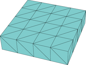
Figure 1: Initial Mesh of Example 1

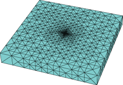
(a) Refined mesh based on $\eta_{{}_{\text{Res},K}}$ cut on $z\!=\!0$

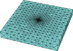
(b) Refined mesh based on $\eta_{{}_{\text{New},K}}$ cut on $z\!=\!0$

Figure 2: Mesh results of Example 1, $\nabla\!\cdot\!\bm{f}=0$

It is easy to see that the exact solution of the auxiliary problem in (3.1) for this example is $\bm{\sigma}=\mu^{-1}\nabla\!\times\!\bm{u}={\bf 0}$. Hence, the true error for the finite element approximation to (3.1) is simply the energy norm of the finite element solution $\bm{\sigma}_{{}_{\mathcal{T}}}$ defined in (3.3)

$$\mathopen{|\mkern-2.5mu|\mkern-2.5mu|}\bm{\sigma}-\bm{\sigma}_{{}_{\mathcal{T}}}\mathclose{|\mkern-2.5mu|\mkern-2.5mu|}_{\mu,\beta}^{2}=\mathopen{|\mkern-2.5mu|\mkern-2.5mu|}\bm{\sigma}_{{}_{\mathcal{T}}}\mathclose{|\mkern-2.5mu|\mkern-2.5mu|}_{\mu,\beta}^{2}=\left\|{\beta^{-1/2}\nabla\!\times\!\bm{\sigma}_{{}_{\mathcal{T}}}}\right\|^{2}+\left\|{\mu^{1/2}\bm{\sigma}_{{}_{\mathcal{T}}}}\right\|^{2}.$$

In the first experiment, we choose the coefficients $\mu=1$ and $\beta=\alpha$. This choice enables that $\nabla\!\cdot\!\bm{f}=0$, i.e., $\bm{f}\in\bm{H}(\operatorname{div};\Omega)$, and that $\bm{u}$ satisfies the $\beta$-weighted normal continuity:

$$[[{\beta\bm{u}\cdot\bm{n}}]]_{\raisebox{-2.0pt}{\scriptsize$F$}}=0$$ (5.1)

for any surface $F$ in the domain $\Omega$. This is the prerequisite for establishing efficiency and reliability bounds in [3] and [6] and the base for recovering $\bm{\tau}_{h}$ in $\bm{\mathcal{B}\!{\mathcal{D}}\!\mathcal{M}}_{1}\subset\bm{H}(\operatorname{div};\Omega)$ in [6]. The quasi-monotonicity assumption is not met in this situation (for the analysis of the quasi-monotonicity affects the robustness of the estimator for $\bm{H}(\mathbf{curl}\hskip 0.7pt)$ problems, please refer to [6]).

The meshes generated by $\eta_{{}_{\text{New},K}}$, $\eta_{{}_{\text{Res},K}}$, and $\eta_{{}_{\text{Rec},K}}$ are almost the same (see Figure 2). In terms of the convergence, we observe that the error estimator $\eta_{{}_{\text{New}}}$ exhibits asymptotical exactness. This is impossible for the error estimators in [3] and [6] because of the presence of the element residuals. Table 1 shows that the number of the DoF for the $\eta_{{}_{\text{New}}}$ is about $30\%$ less than those of the other two estimators while achieving a better accuracy. As the reliability of the estimator does not depend on the quasi-monotonicity of the coefficient, the rate of the convergence is not hampered by checkerboard pattern of the $\beta$.

Table 1: Estimators Comparison, Example 1, $\nabla\!\cdot\!\bm{f}=0$

	# Iter	# DoF	error	rel-error	$\eta$	eff-index
$\eta_{{}_{\text{Res}}}$	$27$	$181324$	$0.0428$	$0.0494$	$0.0953$	$2.226$
$\eta_{{}_{\text{Rec}}}$	$27$	$187287$	$0.0421$	$0.0486$	$0.0428$	$1.041$
$\eta_{{}_{\text{New}}}$	$24$	$127857$	$0.0411$	$0.0473$	$0.0405$	$0.985$
$\widetilde{\eta}_{{}_{\text{New}}}$	$25$	$129564$	$0.0418$	$0.0482$	$0.0479$	$1.147$

In the second experiment, we choose that $\mu=\beta=1$. Due to the fact that the normal component of $\bm{u}=\nabla\psi$ is discontinuous across the interfaces, the exact solution $\bm{u}$ does not satisfy the usual $\beta$-weighted normal continuity (5.1), i.e.,

$$[[{\beta\bm{u}\cdot\bm{n}}]]_{\raisebox{-2.0pt}{\scriptsize$F$}}\neq 0.$$

This leads to a right-hand side $\bm{f}=\beta\bm{u}=\nabla\psi$ that is not in $\bm{H}(\operatorname{div};\Omega)$ in the primary problem. Even though the $\bm{H}(\operatorname{div})$-continuity is required for establishing the reliability and efficiency of the existing residual-based and recovery-based estimators, the old residual-based and recovery-based estimators may still be used if $\nabla\!\cdot\!\bm{f}\big{|}_{\raisebox{-0.5pt}{\scriptsize$K$}}\in\bm{L}^{2}(K)$ for all $K\in{\mathcal{T}}$. Therefore, we implement all three estimators in this experiment as well.

Table 2: Estimators Comparison, Example 1, $\bm{f}\notin\bm{H}(\operatorname{div};\Omega)$

	# Iter	# DoF	error	rel-error	$\eta$	eff-index
$\eta_{{}_{\text{Res}}}$	$31$	$247003$	$0.0337$	$0.0507$	$0.115$	$3.420$
$\eta_{{}_{\text{Rec}}}$	$24$	$218497$	$0.0355$	$0.0534$	$0.0559$	$1.577$
$\eta_{{}_{\text{New}}}$	$22$	$99215$	$0.0342$	$0.0514$	$0.0329$	$0.964$
$\widetilde{\eta}_{{}_{\text{New}}}$	$24$	$103419$	$0.0338$	$0.0508$	$0.0434$	$1.283$

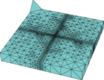
(a) Refined Mesh based on $\eta_{{}_{\text{Res},K}}$ cut on $z=0$

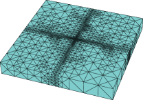
(b) Refined Mesh based on $\eta_{{}_{\text{Rec},K}}$ cut on $z=0$

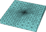
(c) Refined Mesh based on $\eta_{{}_{\text{New},K}}$ cut on $z=0$

Figure 3: Mesh Result of Example 1, $\bm{f}\notin\bm{H}(\operatorname{div};\Omega)$

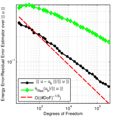
(a) Convergence of $\eta_{{}_{\text{Res}}}$

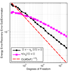
(b) Convergence of $\eta_{{}_{\text{Rec}}}$

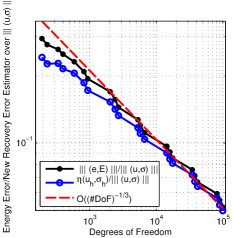
(c) Convergence of $\eta_{{}_{\text{New}}}$

Figure 4: Convergence Results of Example 1, $\bm{f}\notin\bm{H}(\operatorname{div};\Omega)$

For the new estimator $\eta_{{}_{\text{New}}}$, it is shown in Figure 4 that the rate of convergence is optimal and that the relative true error and the relative estimator is approximately equal.

Table 2 indicates that the number of the degrees of freedom using the $\eta_{{}_{\text{New}}}$ is less than half of those using the other two estimators. This is confirmed by the meshes depicted in Figure 3 where both the $\eta_{{}_{\text{Res}}}$ and $\eta_{{}_{\text{Rec}}}$ over-refine meshes along the interfaces, where there are no errors. Such inefficiency of the estimators $\eta_{{}_{\text{Res}}}$ and $\eta_{{}_{\text{Rec}}}$ is also shown in Figure 4 through the non-optimal rate of convergence. Moreover, Figure 4 shows that both the $\eta_{{}_{\text{Res}}}$ and $\eta_{{}_{\text{Rec}}}$ are not reliable because the slopes of the relative error and the relative estimator are different. The main reason for this failure is due to the normal jump term $h_{F}^{1/2}\left\|{[[{\beta\bm{u}_{{}_{\mathcal{T}}}\cdot\bm{n}}]]_{\raisebox{-2.0pt}{\scriptsize$F$}}}\right\|_{F}$ along the interfaces, which is bigger than the true error.

Example 2: In this example, the performance of the estimators for solenoidal vector field is investigated. Like the first example, the coefficients distribution across the computational domain is in a checkerboard pattern, not satisfying the quasi-monotonicity either. The computational domain $\overline{\Omega}=[-1,1]^{3}=\overline{\Omega}_{1}\cap\overline{\Omega}_{0}$, and $\mu$ is given by:

$$\mu=\begin{cases}a&\text{ in }\Omega_{1},\\ 1&\text{ in }\Omega_{0}.\end{cases}$$

where $\Omega_{1}=\{(x,y,z)\in\mathbb{R}^{3}:xyz>0\}\cap\Omega$ and $\Omega_{0}=\{(x,y,z)\in\mathbb{R}^{3}:xyz\leq 0\}\cap\Omega$. The true solution is given by

$$\bm{u}=\mu\big{(}\sin(\pi yz),\sin(\pi xz),\sin(\pi xy)\big{)}.$$

Table 3: Estimators Comparison, Example 2, $\nabla\!\cdot\!\bm{f}=0$

	# Iter	# DoF	error	rel-error	$\eta$	eff-index
$\eta_{{}_{\text{Res}}}$	$34$	$118740$	$0.368$	$0.0699$	$0.793$	$2.157$
$\eta_{{}_{\text{Rec}}}$	$22$	$120550$	$0.365$	$0.0677$	$0.644$	$1.762$
$\eta_{{}_{\text{New}}}$	$25$	$50080$	$1.500$	$0.0681$	$1.490$	$0.993$
$\widetilde{\eta}_{{}_{\text{New}}}$	$26$	$51745$	$1.526$	$0.0693$	$1.763$	$1.155$

In the first experiment, the $\beta$ is given as follows:

$$\beta=\begin{cases}a^{-1}&\text{ in }\Omega_{1},\\ 1&\text{ in }\Omega_{0},\end{cases}$$

where $a=10^{-3}$. This choice makes $\nabla\cdot\bm{f}=0$, and the true solution $\bm{u}$ satisfies both the tangential continuity and the normal continuity (5.1). Similarly to the first example, the meshes refined using three error estimators exhibit no significant difference. Yet, the new estimator again shows the asymptotically exactness behavior as Example 1 (see Figure 5), and requires much less degrees of freedom to achieve the same level of relative error. For the results please refer to Table 3.

Table 4: Estimators Comparison, Example 2, $\bm{f}\notin\bm{H}(\operatorname{div};\Omega)$

	# Iter	# DoF	error	rel-error	$\eta$	eff-index
$\eta_{{}_{\text{Res}}}$	$31$	$153352$	$4.495$	$0.0699$	$18.165$	$4.041$
$\eta_{{}_{\text{Rec}}}$	$29$	$159194$	$4.538$	$0.0664$	$9.857$	$2.172$
$\eta_{{}_{\text{New}}}$	$24$	$49894$	$5.263$	$0.0684$	$5.254$	$0.998$
$\widetilde{\eta}_{{}_{\text{New}}}$	$25$	$57338$	$4.945$	$0.0642$	$6.087$	$1.231$

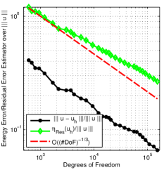
(a) Convergence of $\eta_{{}_{\text{Res}}}$

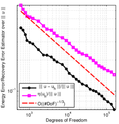
(b) Convergence of $\eta_{{}_{\text{Rec}}}$

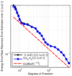
(c) Convergence of $\eta_{{}_{\text{New}}}$

Figure 5: Convergence Results of Example 2, $\bm{f}\notin\bm{H}(\operatorname{div};\Omega)$

In the second experiment, the $\beta$ is chosen to be:

$$\beta=\begin{cases}1&\text{ in }\Omega_{1},\\ a^{-1}&\text{ in }\Omega_{0}.\end{cases}$$

We test the case where $a=10^{-3}$. Similar to Example 1, the necessary tangential jump conditions across the interfaces for the primary problem are satisfied. Yet the choice of $\beta$ implies that the right hand side $\bm{f}\notin\bm{H}(\operatorname{div};\Omega)$. Using the residual-based or recovery-based estimator will again lead to unnecessary over-refinement along the interfaces (see Figure 6), and the order of convergence is sub-optimal than the optimal order for linear elements (See Table 4 and Figure 5).

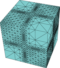
(a) Adaptively refined mesh based on $\eta_{{}_{\text{Res},K}}$

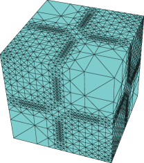
(b) Adaptively refined mesh based on $\eta_{{}_{\text{Rec},K}}$

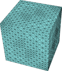
(c) Adaptively refined mesh based on $\eta_{{}_{\text{New},K}}$

Figure 6: Mesh Result of Example 2, $\bm{f}\notin\bm{H}(\operatorname{div};\Omega)$

The new estimator in this paper shows convergence in the optimal order no matter how we set up the jump of the coefficients. The conclusion of comparison with the other two estimators remains almost the same with Example 1. In this example, the differences are more drastic: $1/3$ the degrees of freedom for the new estimator to get roughly the same level of approximation with the other two.

Appendix A Appendix

In this appendix, an a priori estimate for the mixed boundary value problem with weights is studied following the arguments and notations mainly from [1, 2]. In our study, it is found that, due to the duality pairing on the Neumann boundary and the nature of the trace space of $\bm{H}(\mathbf{curl}\hskip 0.7pt)$, a higher regularity is needed for the Neumann boundary data $\bm{g}_{{}_{N}}$ than those for elliptic mixed boundary value problem. First we define the tangential trace operator and tangential component projection operator, and their range acting on the $\bm{H}_{B}(\mathbf{curl}\hskip 0.7pt;\Omega)$. Secondly we construct a weighted extension of the Dirichlet boundary data to the interior of the domain. Lastly the a priori estimate for the solution of problem (2.1) is established after a trace inequality is set up for the piecewise smooth vector field.

A.1 The tangential trace and tangential component space

On either Dirichlet or Neumann part of the boundary, the tangential trace operator $\gamma_{\top,B}$ and the tangential component operator $\pi_{\top,B}$ are defined as follows:

$$\gamma_{\top,B}:\bm{v}\mapsto\left\{\begin{array}[]{ll}\bm{v}\!\times\!\bm{n}&\mbox{on }\,\Gamma_{B},\\[5.69054pt] \bm{0}&\mbox{on }\,\partial\Omega\backslash\overline{\Gamma}_{B},\end{array}\right.\mbox{and}\,\,\,\pi_{\top,B}:\bm{v}\mapsto\left\{\begin{array}[]{ll}\bm{n}\!\times\!(\bm{v}\!\times\!\bm{n})&\mbox{on }\,\Gamma_{B},\\[5.69054pt] \bm{0}&\mbox{on }\,\partial\Omega\backslash\overline{\Gamma}_{B},\end{array}\right.$$ (A.1)

respectively, where $\Gamma_{B}$ is either $\Gamma_{D}$ or $\Gamma_{N}$.

Define the following spaces as the trace spaces of $\bm{H}(\mathbf{curl}\hskip 0.7pt;\Omega)$:

$$\bm{X}_{\mathop{\mathchoice{\textstyle\mathbin{\!/\mkern-5.0mu/\!}}{\scriptstyle\mathbin{\!/\mkern-5.0mu/\!}}{\scriptscriptstyle\mathbin{\!/\mkern-5.0mu/\!}}{\scriptscriptstyle\mathbin{\!/\mkern-5.0mu/\!}}}\nolimits}(\Gamma_{B}):=\gamma_{\top,B}\bm{H}(\mathbf{curl}\hskip 0.7pt;\Omega)\quad\text{and}\quad\bm{X}_{\perp}(\Gamma_{B}):=\pi_{\top,B}\bm{H}(\mathbf{curl}\hskip 0.7pt;\Omega).$$ (A.2)

For the $\bm{H}^{1}$-regular vector fields, define the trace spaces $\bm{H}^{1/2}_{\mathop{\mathchoice{\textstyle\mathbin{\!/\mkern-5.0mu/\!}}{\scriptstyle\mathbin{\!/\mkern-5.0mu/\!}}{\scriptscriptstyle\mathbin{\!/\mkern-5.0mu/\!}}{\scriptscriptstyle\mathbin{\!/\mkern-5.0mu/\!}}}\nolimits}(\Gamma_{B})$ and $\bm{H}^{1/2}_{\perp}(\Gamma_{B})$ as:

$$\bm{H}^{1/2}_{\mathop{\mathchoice{\textstyle\mathbin{\!/\mkern-5.0mu/\!}}{\scriptstyle\mathbin{\!/\mkern-5.0mu/\!}}{\scriptscriptstyle\mathbin{\!/\mkern-5.0mu/\!}}{\scriptscriptstyle\mathbin{\!/\mkern-5.0mu/\!}}}\nolimits}(\Gamma_{B})=\pi_{\top,B}\bm{H}^{1}(\Omega)\quad\text{and}\quad\bm{H}^{1/2}_{\perp}(\Gamma_{B})=\gamma_{\top,B}\bm{H}^{1}(\Omega).$$ (A.3)

It is proved in [2] that the tangential trace space and the tangential component space can be characterized by

$$\bm{X}_{\mathop{\mathchoice{\textstyle\mathbin{\!/\mkern-5.0mu/\!}}{\scriptstyle\mathbin{\!/\mkern-5.0mu/\!}}{\scriptscriptstyle\mathbin{\!/\mkern-5.0mu/\!}}{\scriptscriptstyle\mathbin{\!/\mkern-5.0mu/\!}}}\nolimits}(\Gamma_{B})\subset\bm{H}^{-1/2}_{\mathop{\mathchoice{\textstyle\mathbin{\!/\mkern-5.0mu/\!}}{\scriptstyle\mathbin{\!/\mkern-5.0mu/\!}}{\scriptscriptstyle\mathbin{\!/\mkern-5.0mu/\!}}{\scriptscriptstyle\mathbin{\!/\mkern-5.0mu/\!}}}\nolimits}(\Gamma_{B})\quad\text{and}\quad\bm{X}_{\perp}(\Gamma_{B})\subset\bm{H}^{-1/2}_{\perp}(\Gamma_{B}).$$ (A.4)

The $-1/2$ supscripted spaces $\bm{H}^{-1/2}_{\mathop{\mathchoice{\textstyle\mathbin{\!/\mkern-5.0mu/\!}}{\scriptstyle\mathbin{\!/\mkern-5.0mu/\!}}{\scriptscriptstyle\mathbin{\!/\mkern-5.0mu/\!}}{\scriptscriptstyle\mathbin{\!/\mkern-5.0mu/\!}}}\nolimits}(\Gamma_{B})$ and $\bm{H}^{-1/2}_{\perp}(\Gamma_{B})$ are defined as the dual spaces of $\bm{H}^{1/2}_{\mathop{\mathchoice{\textstyle\mathbin{\!/\mkern-5.0mu/\!}}{\scriptstyle\mathbin{\!/\mkern-5.0mu/\!}}{\scriptscriptstyle\mathbin{\!/\mkern-5.0mu/\!}}{\scriptscriptstyle\mathbin{\!/\mkern-5.0mu/\!}}}\nolimits}(\Gamma_{B})$ and $\bm{H}^{1/2}_{\perp}(\Gamma_{B})$.

Now we move on to define the weighted divergence integrable space

$$\bm{H}(\operatorname{div};\Omega,\alpha):=\{\bm{v}\in\bm{L}^{2}(\Omega):\nabla\!\cdot\!(\alpha\bm{v})\in L^{2}(\Omega)\text{ in }\Omega\},$$ (A.5)

and $$\bm{H}(\operatorname{div}0\,;\Omega,\alpha):=\{\bm{v}\in\bm{L}^{2}(\Omega):\nabla\!\cdot\!(\alpha\bm{v})=0\text{ in }\Omega\},$$

and the piecewise regular field space $\bm{X}(\Omega,\alpha,\Gamma_{B})$ as follows:

$$\bm{X}(\Omega,\alpha,\Gamma_{B}):={\mathop{{}\bm{H}}\limits^{\vbox to-0.3014pt{\kern-1.50694pt\hbox{$\scriptstyle\circ$}\vss}}}_{B}(\mathbf{curl}\hskip 0.7pt;\Omega)\cap\bm{H}(\operatorname{div};\Omega,\alpha),$$ (A.6)

and $$\bm{X}_{0}(\Omega,\alpha,\Gamma_{B}):={\mathop{{}\bm{H}}\limits^{\vbox to-0.3014pt{\kern-1.50694pt\hbox{$\scriptstyle\circ$}\vss}}}_{B}(\mathbf{curl}\hskip 0.7pt;\Omega)\cap\bm{H}(\operatorname{div}0\,;\Omega,\alpha).$$

The piecewise $\bm{H}^{1}$ vector field space is defined as:

$${P\!\bm{H}}^{1}(\Omega,\mathscr{P})=\{\bm{v}\in\bm{L}^{2}(\Omega):\bm{v}\big{|}_{\raisebox{-0.5pt}{\scriptsize$\Omega_{j}$}}\in\bm{H}^{1}(\Omega_{j}),\,j=1,\ldots,m\}.$$ (A.7)

Assumption A.1 (Boundary Requirement).

Let the Dirichlet or Neumann boundary $\Gamma_{B}$ ($B=D$ or $N$) be decomposed into simply-connected components: $\overline{\Gamma_{B}}=\cup_{i}\overline{\Gamma_{B,i}}$. For any $\Gamma_{B,i}$, there exists a single $j\in\{1,\dots,m\}$, such that $\Gamma_{B,i}\subset\partial\Omega_{j}\cap\partial\Omega$.

Remark A.2.

Assumption A.1 is to say, each connected component on the Dirichlet or Neumann boundary only serves as the boundary of exactly one subdomain. Assumption A.1 is here solely for the a priori error estimate. The robustness of the estimator in Section 5 does not rely on this assumption if the boundary data are piecewise polynomials.

Due to Assumption A.1, the tangential trace and tangential component of a $\bm{H}^{1}(\Omega)$ vector field is the same space as those of a ${P\!\bm{H}}^{1}(\Omega,\mathscr{P})$ vector field on $\Gamma_{D}$ or $\Gamma_{N}$ respectively. With slightly abuse of notation, define

$$\bm{H}^{1/2}_{\mathop{\mathchoice{\textstyle\mathbin{\!/\mkern-5.0mu/\!}}{\scriptstyle\mathbin{\!/\mkern-5.0mu/\!}}{\scriptscriptstyle\mathbin{\!/\mkern-5.0mu/\!}}{\scriptscriptstyle\mathbin{\!/\mkern-5.0mu/\!}}}\nolimits}(\Gamma_{B}):=\pi_{\top,B}{P\!\bm{H}}^{1}(\Omega,\mathscr{P}),\quad\text{and}\quad\bm{H}^{1/2}_{\perp}(\Gamma_{B}):=\gamma_{\top,B}{P\!\bm{H}}^{1}(\Omega,\mathscr{P}).$$ (A.8)

Now we define the weighted $1/2$-norm for the value of any $\bm{v}\in{P\!\bm{H}}^{1}(\Omega,\mathscr{P})\cap\bm{X}(\Omega,\beta,\Gamma_{B})$ on boundary as:

$$\left\|{\bm{v}}\right\|_{1/2,\beta,\mu,\Gamma_{B}}:=\inf_{\bm{v}}\left\{\left\|{\beta^{-1/2}\nabla\!\times\!\bm{v}}\right\|^{2}+\left\|{\mu^{-1/2}\nabla\!\cdot\!(\mu\bm{v})}\right\|^{2}+\left\|{\mu^{1/2}\bm{v}}\right\|^{2}\right\}^{1/2}.$$ (A.9)

Now thanks to the embedding results from [6], $\left\|{\cdot}\right\|_{1/2,\beta,\mu,\Gamma_{B}}$ is equivalent to the unweighted $\left\|{\cdot}\right\|_{1/2,\Gamma_{B}}$ which can be defined as:

$$\left\|{\bm{v}}\right\|_{1/2,\Gamma_{B}}:=\inf_{\bm{v}}\left\{\sum_{j=1}^{m}\left\|{\bm{v}}\right\|_{1,\Omega_{j}}^{2}+\left\|{\bm{v}}\right\|^{2}\right\}^{1/2}.$$

Naturally, the wegithed $-1/2$-norm of any distribution on the boundary can be defined as

$$\left\|{\bm{g}}\right\|_{-1/2,\mu,\beta,\Gamma_{B}}:=\sup_{\bm{v}\in{P\!\bm{H}}^{1}(\Omega,\mathscr{P})\cap\bm{X}(\Omega,\beta,\Gamma_{B})}\frac{{\left\langle{\bm{g}},{\bm{v}}\right\rangle}_{\Gamma_{B}}}{\left\|{\bm{v}}\right\|_{1/2,\beta,\mu,\Gamma_{B}}}.$$ (A.10)

A.2 Extension of The Dirichlet Boundary Data

After the preparation, we are ready to construct the extension operator for any $\bm{g}_{D}\in\bm{X}_{\mathop{\mathchoice{\textstyle\mathbin{\!/\mkern-5.0mu/\!}}{\scriptstyle\mathbin{\!/\mkern-5.0mu/\!}}{\scriptscriptstyle\mathbin{\!/\mkern-5.0mu/\!}}{\scriptscriptstyle\mathbin{\!/\mkern-5.0mu/\!}}}\nolimits}(\Gamma_{D}):=\gamma_{\top,D}\bm{H}(\mathbf{curl}\hskip 0.7pt;\Omega)$.

Lemma A.3.

For any $\bm{g}_{{}_{D}}\in\bm{X}_{\mathop{\mathchoice{\textstyle\mathbin{\!/\mkern-5.0mu/\!}}{\scriptstyle\mathbin{\!/\mkern-5.0mu/\!}}{\scriptscriptstyle\mathbin{\!/\mkern-5.0mu/\!}}{\scriptscriptstyle\mathbin{\!/\mkern-5.0mu/\!}}}\nolimits}(\Gamma_{D})$, there exists an extension $\bm{u}_{{}_{D}}\in\bm{H}_{D}(\mathbf{curl}\hskip 0.7pt;\Omega)$ such that $\gamma_{\top,D}\bm{u}_{{}_{D}}=\bm{g}_{{}_{D}}$, and the following estimate holds

$$\mathopen{|\mkern-2.5mu|\mkern-2.5mu|}\bm{u}_{{}_{D}}\mathclose{|\mkern-2.5mu|\mkern-2.5mu|}_{\mu,\beta}\leq\left\|{\bm{g}_{{}_{D}}}\right\|_{-1/2,\mu,\beta,\Gamma_{D}}.$$ (A.11)

Moreover, for any $\bm{v}\in{\mathop{{}\bm{H}}\limits^{\vbox to-0.3014pt{\kern-1.50694pt\hbox{$\scriptstyle\circ$}\vss}}}_{D}(\mathbf{curl}\hskip 0.7pt;\Omega)$, there holds

$$A_{\mu,\beta}(\bm{u}_{{}_{D}},\bm{v})=0.$$

Proof.

The fact that $\bm{g}_{{}_{D}}\in\bm{X}_{\mathop{\mathchoice{\textstyle\mathbin{\!/\mkern-5.0mu/\!}}{\scriptstyle\mathbin{\!/\mkern-5.0mu/\!}}{\scriptscriptstyle\mathbin{\!/\mkern-5.0mu/\!}}{\scriptscriptstyle\mathbin{\!/\mkern-5.0mu/\!}}}\nolimits}(\Gamma_{D})\subset\bm{H}^{-1/2}_{\mathop{\mathchoice{\textstyle\mathbin{\!/\mkern-5.0mu/\!}}{\scriptstyle\mathbin{\!/\mkern-5.0mu/\!}}{\scriptscriptstyle\mathbin{\!/\mkern-5.0mu/\!}}{\scriptscriptstyle\mathbin{\!/\mkern-5.0mu/\!}}}\nolimits}(\Gamma_{D})$ implies the following problem is well-posed:

$$\left\{\begin{aligned} &\text{Find }\bm{w}\in{P\!\bm{H}}^{1}(\Omega,\mathscr{P})\cap\bm{X}_{0}(\Omega,\mu,\Gamma_{N})\text{ such that:}\\[5.69054pt] &\mathfrak{A}_{\beta,\mu}(\bm{w},\bm{v})={\left\langle{\bm{g}_{D}},{\bm{v}}\right\rangle},\quad\forall\,\bm{v}\in{P\!\bm{H}}^{1}(\Omega,\mathscr{P})\cap\bm{X}_{0}(\Omega,\alpha,\Gamma_{N}),\end{aligned}\right.$$ (A.12)

where the bilinear form $\mathfrak{A}_{\beta,\mu}(\cdot,\cdot)$ is given as

$$\mathfrak{A}_{\beta,\mu}(\bm{w},\bm{v}):=\bigl{(}{\beta^{-1}\nabla\!\times\!\bm{w}},\,{\nabla\!\times\!\bm{v}}\bigr{)}+\bigl{(}{\mu^{-1}\nabla\!\cdot\!(\mu\bm{w})},\,{\nabla\!\cdot\!(\mu\bm{v})}\bigr{)}+\bigl{(}{\mu\bm{w}},\,{\bm{v}}\bigr{)}.$$

On this weighted divergence free subspace ${P\!\bm{H}}^{1}(\Omega,\mathscr{P})\cap\bm{X}_{0}(\Omega,\mu,\Gamma_{N})$:

$$\mathfrak{A}_{\beta,\mu}(\bm{w},\bm{v})=\bigl{(}{\beta^{-1}\nabla\!\times\!\bm{w}},\,{\nabla\!\times\!\bm{v}}\bigr{)}+\bigl{(}{\mu\bm{w}},\,{\bm{v}}\bigr{)}.$$

With slightly abuse of notation, the zero extension of $\bm{g}_{{}_{D}}$ to the Neumann boundary is denoted as $\bm{g}_{{}_{D}}$ itself. Now for the trial function space and the test function space in problem (A.12) are the same, letting $\bm{w}=\bm{v}$ leads to

$$\mathopen{|\mkern-2.5mu|\mkern-2.5mu|}\bm{w}\mathclose{|\mkern-2.5mu|\mkern-2.5mu|}_{\beta,\mu}^{2}={\left\langle{\bm{g}_{{}_{D}}},{\bm{w}}\right\rangle}.$$

Together with their tangential traces vanish on the Neumann boundary, this implies

$$\mathopen{|\mkern-2.5mu|\mkern-2.5mu|}\bm{w}\mathclose{|\mkern-2.5mu|\mkern-2.5mu|}_{\beta,\mu}=\frac{{\left\langle{\bm{g}_{{}_{D}}},{\bm{w}}\right\rangle}}{\mathopen{|\mkern-2.5mu|\mkern-2.5mu|}\bm{w}\mathclose{|\mkern-2.5mu|\mkern-2.5mu|}_{\beta,\mu}}\leq\sup_{\bm{v}}\frac{{\left\langle{\bm{g}_{{}_{D}}},{\bm{v}}\right\rangle}}{\mathopen{|\mkern-2.5mu|\mkern-2.5mu|}\bm{v}\mathclose{|\mkern-2.5mu|\mkern-2.5mu|}_{\beta,\mu}}\leq\sup_{\bm{v}}\frac{{\left\langle{\bm{g}_{{}_{D}}},{\bm{v}}\right\rangle}_{\Gamma_{D}}}{\left\|{\bm{v}}\right\|_{1/2,\beta,\mu,\Gamma_{D}}}=\left\|{\bm{g}_{{}_{D}}}\right\|_{-1/2,\mu,\beta,\Gamma_{D}}.$$

The extension is now letting $\bm{u}_{{}_{D}}=\beta^{-1}\nabla\!\times\!\bm{w}$. To prove the estimate, we first notice that the problem (A.12) is a consistent variational formulation for the following PDE:

$$\left\{\begin{aligned} \nabla\!\times\!(\beta^{-1}\nabla\!\times\!\bm{w})+\mu\,\bm{w}&=\bm{0},&\text{ in }\,\Omega,\;\;\\ \nabla\!\cdot\!(\mu\bm{w})&=0,&\;\text{ in }\,\Omega,\;\;\\ (\mu^{-1}\nabla\!\times\!\bm{w})\!\times\!\bm{n}&=\bm{g}_{{}_{D}},&\;\text{ on }\,\Gamma_{D}.\end{aligned}\right.$$ (A.13)

Therefore, the energy norm of $\bm{u}_{{}_{D}}$ is

$$\mathopen{|\mkern-2.5mu|\mkern-2.5mu|}\bm{u}_{{}_{D}}\mathclose{|\mkern-2.5mu|\mkern-2.5mu|}_{\mu,\beta}^{2} =\left\|{\mu^{-1/2}\nabla\!\times\!\bm{u}_{{}_{D}}}\right\|^{2}+\left\|{\beta^{1/2}\bm{u}_{{}_{D}}}\right\|^{2}$$

$$=\left\|{\mu^{1/2}\bm{w}}\right\|^{2}+\left\|{\beta^{-1/2}\nabla\!\times\!\bm{w}}\right\|^{2}$$

$$=\mathopen{|\mkern-2.5mu|\mkern-2.5mu|}\bm{w}\mathclose{|\mkern-2.5mu|\mkern-2.5mu|}_{\beta,\mu}^{2}\leq\left\|{\bm{g}_{{}_{D}}}\right\|_{-1/2,\mu,\beta,\Gamma_{D}}.$$

For the second equality in the Lemma, it is straightforward to verify that for any $\bm{v}\in{\mathop{{}\bm{H}}\limits^{\vbox to-0.3014pt{\kern-1.50694pt\hbox{$\scriptstyle\circ$}\vss}}}_{D}(\mathbf{curl}\hskip 0.7pt;\Omega)$, with $\bm{w}$ is from the above construction, the following identity holds

$$A_{\mu,\beta}(\bm{u}_{{}_{D}},\bm{v}) =\bigl{(}{\mu^{-1}\nabla\!\times\!\bm{u}_{{}_{D}}},\,{\nabla\!\times\!\bm{v}}\bigr{)}+\bigl{(}{\beta\bm{u}_{{}_{D}}},\,{\bm{v}}\bigr{)}$$

$$=\bigl{(}{-\bm{w}},\,{\nabla\!\times\!\bm{v}}\bigr{)}+\bigl{(}{\nabla\!\times\!\bm{w}},\,{\bm{v}}\bigr{)}$$

$$={\left\langle{\bm{n}\!\times\!\bm{w}},{\bm{v}}\right\rangle}=0.$$

The last equality follows from the fact that $\bm{w}\!\times\!\bm{n}=\bm{0}$ on $\Gamma_{N}$ and $\bm{v}\!\times\!\bm{n}=\bm{0}$ on $\Gamma_{D}$. ∎

A.3 A Trace inequality

In this section we want to establish a trace inequality for the tangential component space of $\bm{H}_{N}(\mathbf{curl}\hskip 0.7pt;\Omega)$. For any $\bm{v}\in{\mathop{{}\bm{H}}\limits^{\vbox to-0.3014pt{\kern-1.50694pt\hbox{$\scriptstyle\circ$}\vss}}}_{D}(\mathbf{curl}\hskip 0.7pt;\Omega)$, consider the tangential component space $\bm{X}_{\perp}(\Gamma_{N})$ defined in (A.2) that contains all the tangential components of $\bm{v}\in{\mathop{{}\bm{H}}\limits^{\vbox to-0.3014pt{\kern-1.50694pt\hbox{$\scriptstyle\circ$}\vss}}}_{D}(\mathbf{curl}\hskip 0.7pt;\Omega)$ on the Neumann boundary and zero on the Dirichlet boundary.

Lemma A.4 (Trace inequality for the tangential component).

For $\bm{v}\in{\mathop{{}\bm{H}}\limits^{\vbox to-0.3014pt{\kern-1.50694pt\hbox{$\scriptstyle\circ$}\vss}}}_{D}(\mathbf{curl}\hskip 0.7pt;\Omega)$, the tangential component of $\bm{v}$ on $\Gamma_{N}$ is $\pi_{\top,N}\bm{v}\in\bm{X}_{\perp}(\Gamma_{N})$ and satisfies the following estimate:

$$\left\|{\pi_{\top,N}\bm{v}}\right\|_{-1/2,\mu,\beta,\Gamma_{N}}\leq\,\mathopen{|\mkern-2.5mu|\mkern-2.5mu|}\bm{v}\mathclose{|\mkern-2.5mu|\mkern-2.5mu|}_{\mu,\beta}.$$ (A.14)

Proof.

First we notice that $\bm{X}_{\perp}(\Gamma_{N})\subset\bm{H}^{-1/2}_{\perp}(\Gamma_{N})$ which is the dual space of $\gamma_{\top,B}{P\!\bm{H}}^{1}(\Omega,\mathscr{P})$. For any $\bm{\xi}\in\bm{H}^{1/2}_{\perp}(\Gamma_{N})$, there exists $\widetilde{\bm{\xi}}\in{P\!\bm{H}}^{1}(\Omega,\mathscr{P})$ such that $\widetilde{\bm{\xi}}\!\times\!\bm{n}\big{|}_{\raisebox{-0.5pt}{\scriptsize$\Gamma_{N}$}}=\bm{\xi}$ and

$$\left\{\left\|{\beta^{-1/2}\nabla\!\times\!\widetilde{\bm{\xi}}}\right\|^{2}+\left\|{\mu^{-1/2}\nabla\!\cdot\!(\mu\widetilde{\bm{\xi}})}\right\|^{2}+\left\|{\mu^{1/2}\widetilde{\bm{\xi}}}\right\|^{2}\right\}^{1/2}\leq\left\|{\bm{\xi}}\right\|_{1/2,\beta,\mu,\Gamma_{N}}.$$

By the integration by parts formula from [2] and Cauchy-Schwarz inequality, we have

$${\left\langle{\bm{\xi}},{\bm{v}}\right\rangle}_{\Gamma_{N}} ={\left\langle{\bm{\xi}},{\pi_{\top,N}\bm{v}}\right\rangle}_{\partial\Omega}$$

$$=\bigl{(}{\nabla\!\times\!\bm{v}},\,{\widetilde{\bm{\xi}}}\bigr{)}-\bigl{(}{\nabla\!\times\!\widetilde{\bm{\xi}}},\,{\bm{v}}\bigr{)}$$

$$=\left\|{\mu^{-1/2}\nabla\!\times\!\bm{v}}\right\|\left\|{\mu^{1/2}\widetilde{\bm{\xi}}}\right\|-\left\|{\beta^{-1/2}\nabla\!\times\!\widetilde{\bm{\xi}}}\right\|\left\|{\beta^{1/2}\bm{v}}\right\|$$

$$\leq\mathopen{|\mkern-2.5mu|\mkern-2.5mu|}\bm{v}\mathclose{|\mkern-2.5mu|\mkern-2.5mu|}_{\mu,\beta}\,\mathopen{|\mkern-2.5mu|\mkern-2.5mu|}\widetilde{\bm{\xi}}\mathclose{|\mkern-2.5mu|\mkern-2.5mu|}_{\beta,\mu}\leq\mathopen{|\mkern-2.5mu|\mkern-2.5mu|}\bm{v}\mathclose{|\mkern-2.5mu|\mkern-2.5mu|}_{\mu,\beta}\,\left\|{\bm{\xi}}\right\|_{1/2,\beta,\mu,\Gamma_{N}}.$$

Hence by definition (A.10) the Lemma follows. ∎

A.4 An A Priori Estimate for the $\bm{H}(\mathbf{curl}\hskip 0.7pt)$ Mixed Boundary Value Problem

Theorem A.5.

Assume that $\bm{f}\in\bm{L}^{2}(\Omega)$, $\bm{g}_{{}_{D}}\in\bm{X}_{\mathop{\mathchoice{\textstyle\mathbin{\!/\mkern-5.0mu/\!}}{\scriptstyle\mathbin{\!/\mkern-5.0mu/\!}}{\scriptscriptstyle\mathbin{\!/\mkern-5.0mu/\!}}{\scriptscriptstyle\mathbin{\!/\mkern-5.0mu/\!}}}\nolimits}(\Gamma_{D})$, and $\bm{g}_{{}_{N}}\in\bm{H}^{1/2}_{\perp}(\Gamma_{N})$. Then the weak formulation of (1.1) has a unique solution $\bm{u}\in\bm{H}_{D}(\mathbf{curl}\hskip 0.7pt;\Omega)$ satisfying the following a priori estimate

$$\mathopen{|\mkern-2.5mu|\mkern-2.5mu|}\bm{u}\mathclose{|\mkern-2.5mu|\mkern-2.5mu|}_{\mu,\beta}\leq\|{\beta^{-1/2}\bm{f}}\|+\left\|{\bm{g}_{{}_{D}}}\right\|_{-1/2,\mu,\beta,\Gamma_{D}}+\left\|{\bm{g}_{{}_{N}}}\right\|_{1/2,\beta,\mu,\Gamma_{N}}.$$ (A.15)

Proof.

Let $\bm{u}_{{}_{D}}\in\bm{H}_{D}(\mathbf{curl}\hskip 0.7pt;\Omega)$ be the extension of the $\bm{g}_{{}_{D}}$ to the domain $\Omega$ from Lemma A.3 such that

$$\begin{gathered}\bm{u}_{{}_{D}}\!\times\!\bm{n}\big{|}_{\raisebox{-0.5pt}{\scriptsize$\Gamma_{D}$}}=\bm{g}_{{}_{D}},\quad\bm{u}_{{}_{D}}\!\times\!\bm{n}\big{|}_{\raisebox{-0.5pt}{\scriptsize$\Gamma_{N}$}}=\bm{0},\\ A_{\mu,\beta}(\bm{u}_{{}_{D}},\bm{v})=0,\quad\mbox{and}\quad\mathopen{|\mkern-2.5mu|\mkern-2.5mu|}\bm{u}_{{}_{D}}\mathclose{|\mkern-2.5mu|\mkern-2.5mu|}_{\mu,\beta}\leq\left\|{\bm{g}_{{}_{D}}}\right\|_{-1/2,\mu,\beta,\Gamma_{D}}.\end{gathered}$$ (A.16)

Now let $\bm{u}=\bm{u}_{0}+\bm{u}_{{}_{D}}$, then $\bm{u}_{0}\in{\mathop{{}\bm{H}}\limits^{\vbox to-0.3014pt{\kern-1.50694pt\hbox{$\scriptstyle\circ$}\vss}}}_{D}(\mathbf{curl}\hskip 0.7pt;\Omega)$ satisfies

$$A_{\mu,\beta}(\bm{u}_{0},\bm{v})=f_{{}_{N}}(\bm{v}),\quad\forall\;\bm{v}\in{\mathop{{}\bm{H}}\limits^{\vbox to-0.3014pt{\kern-1.50694pt\hbox{$\scriptstyle\circ$}\vss}}}_{D}(\mathbf{curl}\hskip 0.7pt;\Omega).$$ (A.17)

The triangle inequality and (A.16) give

$$\mathopen{|\mkern-2.5mu|\mkern-2.5mu|}\bm{u}\mathclose{|\mkern-2.5mu|\mkern-2.5mu|}_{\mu,\beta}\leq\mathopen{|\mkern-2.5mu|\mkern-2.5mu|}\bm{u}_{0}\mathclose{|\mkern-2.5mu|\mkern-2.5mu|}_{\mu,\beta}+\mathopen{|\mkern-2.5mu|\mkern-2.5mu|}\bm{u}_{{}_{D}}\mathclose{|\mkern-2.5mu|\mkern-2.5mu|}_{\mu,\beta}\leq\mathopen{|\mkern-2.5mu|\mkern-2.5mu|}\bm{u}_{0}\mathclose{|\mkern-2.5mu|\mkern-2.5mu|}_{\mu,\beta}+\left\|{\bm{g}_{{}_{D}}}\right\|_{-1/2,\mu,\beta,\Gamma_{D}}.$$

Now, to show the validity of the theorem, it suffices to prove that problem (A.17) has a unique solution $\bm{u}_{0}\in{\mathop{{}\bm{H}}\limits^{\vbox to-0.3014pt{\kern-1.50694pt\hbox{$\scriptstyle\circ$}\vss}}}_{D}(\mathbf{curl}\hskip 0.7pt;\Omega)$ satisfying the following a priori estimate

$$\mathopen{|\mkern-2.5mu|\mkern-2.5mu|}\bm{u}_{0}\mathclose{|\mkern-2.5mu|\mkern-2.5mu|}_{\mu,\beta}\leq\left\|{\beta^{-1/2}\bm{f}}\right\|+\left\|{\bm{g}_{{}_{N}}}\right\|_{1/2,\beta,\mu,\Gamma_{N}}.$$ (A.18)

To this end, for any $\bm{v}\in{\mathop{{}\bm{H}}\limits^{\vbox to-0.3014pt{\kern-1.50694pt\hbox{$\scriptstyle\circ$}\vss}}}_{D}(\mathbf{curl}\hskip 0.7pt;\Omega)$, we have from trace Lemma A.4

$$\left\|{\pi_{\top,N}\bm{v}}\right\|_{-1/2,\mu,\beta,\Gamma_{N}}\leq\mathopen{|\mkern-2.5mu|\mkern-2.5mu|}\bm{v}\mathclose{|\mkern-2.5mu|\mkern-2.5mu|}_{\mu,\beta},$$

which, together with the Cauchy-Schwarz inequality, implies

$$|f_{{}_{N}}(\bm{v})| \leq \left\|{\beta^{-1/2}\bm{f}}\right\|\,\left\|{\beta^{1/2}\bm{v}}\right\|+\left\|{\bm{g}_{{}_{N}}}\right\|_{1/2,\beta,\mu,\Gamma_{N}}\left\|{\pi_{\top,N}\bm{v}}\right\|_{-1/2,\mu,\beta,\Gamma_{N}}$$

$$\leq \left(\left\|{\beta^{-1/2}\bm{f}}\right\|+\left\|{\bm{g}_{{}_{N}}}\right\|_{1/2,\beta,\mu,\Gamma_{N}}\right)\mathopen{|\mkern-2.5mu|\mkern-2.5mu|}\bm{v}\mathclose{|\mkern-2.5mu|\mkern-2.5mu|}_{\mu,\beta}.$$

By the Lax-Milgram lemma, (A.17) has a unique solution $\bm{u}_{0}\in{\mathop{{}\bm{H}}\limits^{\vbox to-0.3014pt{\kern-1.50694pt\hbox{$\scriptstyle\circ$}\vss}}}_{D}(\mathbf{curl}\hskip 0.7pt;\Omega)$. Taking $\bm{v}=\bm{u}_{0}$ in (A.17), we have

$$\mathopen{|\mkern-2.5mu|\mkern-2.5mu|}\bm{u}_{0}\mathclose{|\mkern-2.5mu|\mkern-2.5mu|}_{\mu,\beta}^{2}=f_{{}_{N}}(\bm{u}_{0})\leq\left(\left\|{\beta^{-1/2}\bm{f}}\right\|+\left\|{\bm{g}_{{}_{N}}}\right\|_{1/2,\beta,\mu,\Gamma_{N}}\right)\mathopen{|\mkern-2.5mu|\mkern-2.5mu|}\bm{u}_{0}\mathclose{|\mkern-2.5mu|\mkern-2.5mu|}_{\mu,\beta}.$$

Dividing $\mathopen{|\mkern-2.5mu|\mkern-2.5mu|}\bm{u}_{0}\mathclose{|\mkern-2.5mu|\mkern-2.5mu|}_{\mu,\beta}$ on the both sides of the above inequality yields (A.18). This completes the proof of the theorem. ∎

References

- [1] A. Alonso and A. Valli, Some remarks on the characterization of the space of tangential traces of H (rot; ) and the construction of an extension operator, Manuscripta Mathematica, 89-1 (1996), 159–178.
- [2] A. Buffa and P. Ciarlet, Jr, On traces for functional spaces related to Maxwell’s equations Part I: An integration by parts formula in Lipschitz polyhedra, Math. Method. Appl. Sci., 24-1 (2001), 9–30.
- [3] R. Beck, R. Hiptmair, R. W. Hoppe, and B. Wohlmuth, Residual based a posteriori error estimators for eddy current computation, Math. Model. Numer. Anal., 34 (2000), 159–182.
- [4] D. Braess and J. Schöberl, Equilibrated residual error estimator for edge elements, Math. Comp., 77 (2008), 651–672.
- [5] Z. Cai and S. Zhang, Robust equilibrated residual error estimator for diffusion problems: Conforming elements, SIAM J. Numer. Anal., 50 (2012), pp. 151–170.
- [6] Z. Cai and S. Cao, A recovery-based a posteriori error estimator for interface problems, Comput. Methods Appl. Mech. Engrg., 296 (2015), 169-195.
- [7] Z. Cai and S. Zhang, Recovery-based error estimators for interface problems: conforming linear elements, SIAM J. Numer. Anal., 47-3 (2009), 2132–2156.
- [8] Z. Cai and S. Zhang, Recovery-based error estimators for interface problems: Mixed and nonconforming finite elements, SIAM J. Numer. Anal., 48 (2010), 30–52.
- [9] L. Chen, FEM: an innovative finite element methods package in MATLAB, Technical Report, University of California at Irvine, (2009).
- [10] J. Chen, Y. Xu, and J. Zou, An adaptive edge element method and its convergence for a saddle-point problem from magnetostatics, Numer. Methods PDEs, 28 (2012), 1643–1666.
- [11] J. Chen, Y. Xu, and J. Zou, Convergence analysis of an adaptive edge element method for Maxwell’s equations, Appl. Numer. Math., 59 (2009), 2950–2969.
- [12] L. Zhong, S. Shu, L. Chen, and J. Xu, Convergence of adaptive edge finite element methods for -elliptic problems, Numerical Linear Algebra with Applications, 17 (2010), 415–432.
- [13] B. Cockburn and J. Gopalakrishnan, Incompressible finite elements via hybridization. Part II: The Stokes system in three space dimensions, SIAM J. Numer. Anal., 43-4 (2005), 1651–1672.
- [14] L. Demkowicz, J. Gopalakrishnan, and J. Schöberl, Polynomial extension operators. Part II, SIAM J. Numer. Anal., 47-5 (2009), 3293–3324.
- [15] I. Ekeland and R. Temam, Convex Analysis and Variational Problems, North-Holland, Amsterdam,1976.
- [16] A. Ern and J.-L. Guermond, Mollification in strongly Lipschitz domains with application to continuous and discrete De Rham complex, arXiv:1509.01325 [math.NA].
- [17] R. Falgout and U. Yang, hypre: A library of high performance preconditioners, Computational Science-ICCS 2002, (2002), 632–641.
- [18] F. Izsák, D. Harutyunyan, and J. J. W. van der Vegt, Implicit a posteriori error estimates for the Maxwell equations, Math. Comp., 77 (2008), 1355–1386.
- [19] R. Hiptmair, Multigrid method for Maxwell’s equations, SIAM J. Numer. Anal., 36-1 (1998), 204–225.
- [20] R. Hiptmair and J. Xu, Nodal auxiliary space preconditioning in H(curl) and H(div) spaces, SIAM J. Numer. Anal., 45-6 (2007), 2483–2509.
- [21] A. Knyazev, M. Argentati, I. Lashuk, E. Ovtchinnikov, Block locally optimal preconditioned eigenvalue xolvers (BLOPEX) in HYPRE and PETSc, SIAM Journal on Scientific Computing, 29-5 (2007), 2224–2239.
- [22] T. Kolev and P. Vassilevski, Some experience with a -based auxiliary space AMG for problems, Lawrence Livermore Nat. Lab., Livermore, CA, Rep. UCRL-TR-221841, 2006.
- [23] MFEM: Modular finite element methods, mfem.org.
- [24] P. Monk, Finite Element Methods for Maxwell’s Equations, Oxford University Press, 2003.
- [25] J.-C. Nédélec, Mixed finite elements in , Numer. Math., 35 (1980), 315–341.
- [26] P. Neittaanmäki and S. Repin, Guaranteed error bounds for conforming approximations of a Maxwell type problem, Applied and Numerical Partial Differential Equations, (2010), pp. 199–211.
- [27] E. Creusé and S. Nicaise, A posteriori error estimation for the heterogeneous Maxwell equations on isotropic and anisotropic meshes, Calcolo, 40-4 (2003), 249–271.
- [28] S. Nicaise, On Zienkiewicz-Zhu error estimators for Maxwell’s equations, C. R. Acad. Sci., Paris, Sér. I, 340 (2005), 697–702.
- [29] S. Cochez-Dhondt and S. Nicaise, Robust a posteriori error estimation for the Maxwell equations, Comput. Methods Appl. Mech. Engrg., 196 (2007), 2583–2595.
- [30] J.T. Oden and L. Demkowicz and W. Rachowicz and T.A. Westermann, Toward a universal hp adaptive finite element strategy, Part 2. A posteriori error estimation, Comput. Methods Appl. Mech. Engrg., 77-1 (1989), 113–180.
- [31] S. Repin, Functional a posteriori estimates for Maxwell’s equation, Journal of Mathematical Sciences, 142-1 (2007), 1821–1827.
- [32] M. Petzoldt, A posteriori error estimators for elliptic equations with discontinuous coefficients, Advances in Computational Mathematics, 16(2002), pp. 47–75.
- [33] W. Prager and J.L. Synge, Approximations in elasticity based on the concept of function space, Quart. Appl. Math, 5-3(1947), pp. 241–269.
- [34] J. Schöberl, A posteriori error estimates for Maxwell equations, Math. Comp., 77 (2008), 633–649.