Horizon of quantum black holes in various dimensions

Abstract

We adapt the horizon wave-function formalism to describe massive static spherically symmetric sources in a general $(1+D)$-dimensional space-time, for $D>3$ and including the $D=1$ case. We find that the probability $P_{\rm BH}$ that such objects are (quantum) black holes behaves similarly to the probability in the $(3+1)$ framework for $D>3$. In fact, for $D\geq 3$, the probability increases towards unity as the mass grows above the relevant $D$-dimensional Planck scale $m_{D}$. At fixed mass, however, $P_{\rm BH}$ decreases with increasing $D$, so that a particle with mass $m\simeq m_{D}$ has just about $10\%$ probability to be a black hole in $D=5$, and smaller for larger $D$. This result has a potentially strong impact on estimates of black hole production in colliders. In contrast, for $D=1$, we find the probability is comparably larger for smaller masses, but $P_{\rm BH}<0.5$, suggesting that such lower dimensional black holes are purely quantum and not classical objects. This result is consistent with recent observations that sub-Planckian black holes are governed by an effective two-dimensional gravitation theory. Lastly, we derive Generalised Uncertainty Principle relations for the black holes under consideration, and find a minimum length corresponding to a characteristic energy scale of the order of the fundamental gravitational mass $m_{D}$ in $D>3$. For $D=1$ we instead find the uncertainty due to the horizon fluctuations has the same form as the usual Heisenberg contribution, and therefore no fundamental scale exists.

1 Introduction

Unusual causal structures like trapping surfaces and horizons can only occur in strongly gravitating systems, such as astrophysical objects that collapse and possibly form black holes. One might argue that for a large black hole, gravity should appear “locally weak” at the horizon, since tidal forces look small to a freely falling observer (their magnitude being roughly controlled by the surface gravity, which is inversely proportional to the horizon radius). Like any other classical signal, light is confined inside the horizon no matter how weak such forces may appear to a local observer. This can be taken as the definition of a “globally strong” interaction.

As the black hole’s mass approaches the Planck scale, tidal forces become strong both in the local and global sense, thus granting such an energy scale a remarkable role in the search for a quantum theory of gravity. It is indeed not surprising that modifications to the standard commutators of quantum mechanics and Generalised Uncertainty Principles (GUPs) have been proposed, essentially in order to account for the possible existence of small black holes around the Planck scale, and the ensuing minimum measurable length [1]. Unfortunately, that regime is presently well beyond our experimental capabilities, at least if one takes the Planck scale at face value , $m_{\rm p}\simeq 10^{16}\,$TeV (corresponding to a length scale $\ell_{\rm p}=\hbar/m_{\rm p}=m_{\rm p}\,G_{\rm N}\simeq 10^{-35}\,$m). Nonetheless, there is the possibility that the low energy theory still retains some signature features that could be accessed in the near future (see, for example, Refs. [2]).

1.1 Gravitational radius and horizon wave-function

Before we start calculating phenomenological predictions, it is of the foremost importance that we clarify the possible conceptual issues arising from the use of arguments and observables that we know work at our every-day scales. One of such key concepts is the gravitational radius of a self-gravitating source, which can be used to assess the existence of trapping surfaces, at least in spherically symmetric systems. As it is very well known, the location of a trapping surface is determined by the equation

$$g^{ij}\nabla_{i}r\nabla_{j}r\,=\,0\ ,$$ (1.1)

where $\nabla_{i}r$ is perpendicular to surfaces of constant area $\mathcal{A}=4\pi r^{2}$. If we set $x^{1}=t$ and $x^{2}=r$, and denote the matter density as $\rho=\rho(r,t)$, the Einstein field equations tell us that

$$g^{rr}\,=\,1-\frac{2\ell_{\rm p}(m/m_{\rm p})}{r}\ ,$$ (1.2)

where the Misner-Sharp mass is given by

$$m(r,t)\,=\,4\pi\int_{0}^{r}\rho(\bar{r},t)\bar{r}^{2}\,\mbox{${\rm d}$}\bar{r}\ ,$$ (1.3)

as if the space inside the sphere were flat. A trapping surface then exists if there are values of $r$ and $t$ such that the gravitational radius $R_{\rm S}=2\,\ell_{\rm p}\,{m}/{m_{\rm p}}\ ,$ satisfies

$$R_{\rm S}(r,t)\,\geq\,r\ .$$ (1.4)

When the above relation holds in the vacuum outside the region where the source is located, $R_{\rm S}$ becomes the usual Schwarzschild radius, and the above argument gives a mathematical foundation to Thorne’s hoop conjecture [3], which (roughly) states that a black hole forms when the impact parameter $b$ of two colliding small objects is shorter than the Schwarzschild radius of the system, that is for $b\lesssim 2\,\ell_{\rm p}\,E/m_{\rm p}$ where $E$ is the total energy in the centre-of mass frame.

If we consider a spin-less point-particle of mass $m$, the Heisenberg principle of quantum mechanics introduces an uncertainty in the particle’s spatial localisation of the order of the Compton scale $\lambda_{m}\simeq\ell_{\rm p}\,m_{\rm p}/m$ . Since quantum physics is a more refined description of reality, we could argue that $R_{\rm S}$ only makes sense if 

$$R_{\rm S}\,\gtrsim\,\lambda_{m}\quad\Longrightarrow\quad m\,\gtrsim\,m_{\rm p}\ ,$$ (1.5)

which brings us to face the conceptual challenge of describing quantum mechanical systems whose classical horizon would be smaller than the size of the uncertainty in their position. In Refs. [6], a proposal was put forward in order to describe the “fuzzy” Schwarzschild (or gravitational) radius of a localised but likewise fuzzy quantum source. One starts from the spectral decomposition of the spherically symmetric wave-function

$$\Ket{\psi_{\rm S}}=\sum_{E}C(E)\Ket{\psi_{E}}\ ,$$ (1.6)

with the usual constraint

$$\hat{H}\Ket{\psi_{E}}=E\Ket{\psi_{E}}\ ,$$ (1.7)

and associates to each energy level $\Ket{\psi_{\rm E}}$ a probability amplitude $\psi_{\rm H}(R_{\rm S})\simeq C(E)$, where $R_{\rm S}=2\,\ell_{\rm p}\,E/m_{\rm p}$. From this Horizon Wave-Function (HWF), a GUP and minimum measurable length were derived [7], as well as corrections to the classical hoop conjecture [8], and a modified time evolution proposed [9]. The same approach was generalised to electrically charged sources [10], and used to show that Bose-Einstein condensate models of black holes [11, 12, 13, 14, 15] actually possess a horizon with a proper semiclassical limit [16].

It is important to emphasise that the HWF approach differs from most previous attempts in which the gravitational degrees of freedom of the horizon, or of the black hole metric, are quantised independently of the nature and state of the source (for some bibliography, see, e.g., Ref. [17]). In our case, the gravitational radius is instead quantised along with the matter source that produces it, somewhat more in line with the highly non-linear general relativistic description of the gravitational interaction. However, having given a practical tool for describing the gravitational radius of a generic quantum system is just the starting point. In fact, when the probability that the source is localised within its gravitational radius is significant, the system should show (some of) the properties ascribed to a black hole in general relativity. These properties, the fact in particular that no signal can escape from the interior, only become relevant once we consider how the overall system evolves.

1.2 Higher and lower dimensional models

Extra-dimensions have been proposed as a possible explanation for some of the incongruences affecting particle physics, such as the hierarchy problem between fundamental interactions. In $(1+D)$-dimensional space-times, with $D\geq 4$, gravity shows its true quantum nature at a scale $m_{D}$ (possibly much) lower than the Planck mass $m_{\rm p}$. Such scenarios have been extensively studied after the well known ADD [18] and Randall-Sundrum [19] models were proposed (see Ref. [20] for a comprehensive review). However our purpose is not to study any model in particular, but to see how the probability of a microscopic black hole formation could be affected by assuming the existence of extra dimensions. We shall therefore just consider black holes in the ADD scenario with a horizon radius significantly shorter than the size of the extra dimensions. It is then important to recall that in these models the Newton constant is replaced by the gravitational constant

$$G_{D}=\frac{\ell_{D}^{D-2}}{m_{D}}\ ,$$ (1.8)

where $\ell_{D}=\hbar/m_{D}\gg\ell_{\rm p}$ is the new gravitational length scale.

On the other hand, gravitational theories become much simpler in space-times with fewer than 3 spatial dimensions, where corresponding quantum theories are exactly solvable [21]. Such theories have been revisited in recent years, motivated by model-independent evidence that the number of space-time dimensions decreases as the Planck length is approached. Such formalisms – known generically as “spontaneous dimension reduction” mechanisms – have been studied in various contexts, mostly focusing on the energy-dependence of the space-time spectral dimension, including causal dynamical triangulations [22] and non-commutative geometry inspired mechanisms [23, 24, 25, 26]. An alternative approach suggests the effective dimensionality of space-time increases as the ambient energy scale drops [27, 28, 29, 30].

Given these arguments, we will generealize the results of Ref. [9] in an arbitrary number of spatial dimensions. In Section 2 we will introduce the concept horizon wave-function and we will apply it to a system described by a gaussian wave-packet. Subsequently, we will compute the probability that the system is a black hole in Section 3 and obtain a Generalised Uncertainty Principle in Section 4. Finally we will give some conclusions and possible outlook about the obtained results in Section 5.

2 Static horizon-wave function in higher dimensions

We recall that, given any spherically symmetric function $f=f(r)$ in $D$ spatial dimensions, the corresponding function in momentum space is given by

$$\tilde{f}(p)\!\! = \!\!\frac{p^{\frac{2-D}{2}}}{\ell_{D}\,m_{D}}\int_{0}^{\infty}\mbox{${\rm d}$}r\,r^{D/2}\,J_{\frac{D-2}{2}}\left(\frac{r\,p}{\ell_{D}\,m_{D}}\right)f(r)\ ,$$ (2.1)

where the normalised radial modes are given by the Bessel functions

$$J_{\frac{D-2}{2}}\left(\frac{r\,p}{\ell_{D}\,m_{D}}\right)=\frac{\Omega_{D-2}}{(2\pi)^{D/2}}\,\left(\frac{r\,p}{\ell_{D}\,m_{D}}\right)^{\frac{D-2}{2}}\int_{0}^{\pi}\mbox{${\rm d}$}\theta\,e^{-i\,p\,r\,\cos\theta/\ell_{D}\,m_{D}}\,(\sin\theta)^{D-2}\ ,$$ (2.2)

and, accordingly, the inverse transform is given by

$${f}(r)=\frac{r^{\frac{2-D}{2}}}{\ell_{D}\,m_{D}}\int_{0}^{\infty}\mbox{${\rm d}$}p\,p^{D/2}\,J_{\frac{D-2}{2}}\left(\frac{r\,p}{\ell_{D}\,m_{D}}\right)\tilde{f}(p)\ .$$ (2.3)

We can apply the above definitions to a localised massive particle described by the Gaussian wave-function

$$\psi_{\rm S}(r)=\frac{e^{-\frac{r^{2}}{2\,\ell^{2}}}}{(\ell\,\sqrt{\pi})^{D/2}}\ ,$$ (2.4)

and the corresponding function in momentum space is thus given by

$$\tilde{\psi}_{\rm S}(p)=\frac{e^{-\frac{p^{2}}{2\,\Delta^{2}}}}{(\Delta\,\sqrt{\pi})^{D/2}}\ ,$$ (2.5)

where $\Delta=m_{D}\,\ell_{D}/\ell$ is the spread of the wave-packet in momenta space.

If we assume

$$\ell\geq\lambda_{m}\equiv\frac{\hbar}{m}=\frac{m_{D}\,\ell_{D}}{m}\ ,$$ (2.6)

where $\lambda_{m}$ is the Compton wavelength, the smallest resolvable scale associated to the particle according to quantum mechanics [4], It immediately follows that $\Delta\leq m$. Note that we have

$$\frac{\ell}{\lambda_{m}}=\frac{m}{\Delta}\ ,$$ (2.7)

which will allow us to express $\Delta$ in terms of $\ell$.

2.1 $(1+D)$-dimensional Schwarzschild metric

The Schwarzschild metric, as a solution of the vacuum Einstein equations, generalises in $(1+D)$-dimensional space-time as

$$ds^{2}=-\left(1-\frac{R_{D}}{r^{D-2}}\right)\,\mbox{${\rm d}$}t^{2}+\left(1-\frac{R_{D}}{r^{D-2}}\right)^{-1}\,\mbox{${\rm d}$}r^{2}+r^{D-1}\,\mbox{${\rm d}$}\Omega_{D-1}\ ,$$ (2.8)

where the classical horizon radius is given by

$$R_{D}=\left(\frac{2\,G_{D}\,M}{|D-2|}\right)^{\frac{1}{D-2}}=\begin{cases}\frac{1}{2\,G_{1}\,M}&\quad\text{if }\ D=1\\ &\\ \left(\frac{2\,G_{D}\,M}{D-2}\right)^{\frac{1}{D-2}}&\quad\text{if }\ D>2\\ \end{cases}\ .$$ (2.9)

Of course, if $D=3$ we have the standard result $R_{3}=R_{\rm S}$. We note that the $D=1$ limit of the horizon radius given above matches that obtained from an exact solution to Einstein’s equations in $(1+1)$-dimensions [31]. We are also purposefully avoiding $(1+2)$-dimensional models, such as the BTZ black holes, because they have meaning only in anti-de Sitter space-time and we are not dealing with a cosmological constant.

As in $D=3$, we assume the relativistic mass-shell relation in flat space [6],

$$p^{2}=E^{2}-m^{2}\ ,$$ (2.10)

and define the HWF expressing the energy $E$ of the particle in terms of the related horizon radius (2.9), $r_{\rm H}=R_{D}(E)$. From Eq. (2.5), we then get

$$\psi_{\rm H}(r_{\rm H})\!\! = \!\!\mathcal{N}_{\rm H}\,\Theta(r_{\rm H}-R_{D})\,\exp\left\{-\frac{1}{2}\left(\frac{D-2}{2\,G_{D}\,\Delta}\right)^{2}\,\left[r_{\rm H}^{2\,(D-2)}-R_{D}^{2\,(D-2)}\right]\right\}\ .$$ (2.11)

The normalisation $\mathcal{N}_{\rm H}$ is fixed according to

$$\mathcal{N}_{\rm H}^{-2}e^{-m^{2}/\Delta^{2}}\!\! = \!\!\frac{\Omega_{D-1}}{\mathcal{N}_{\rm H}^{2}}\,e^{-m^{2}/\Delta^{2}}\,\int_{0}^{\infty}|\psi_{\rm H}(r_{\rm H})|^{2}\,r_{\rm H}^{D-1}\,\mbox{${\rm d}$}r_{\rm H}$$ (2.12)

$$= \!\!\frac{\pi^{D/2}}{D-2}\,\left(\frac{2G_{D}\Delta}{D-2}\right)^{\frac{D}{D-2}}\,\frac{\Gamma\left(\frac{D}{2D-4},\frac{m^{2}}{\Delta^{2}}\right)}{\Gamma\left(\frac{D}{2}\right)}\ ,$$

where

$$\Gamma(s,x)=\int_{x}^{\infty}t^{s-1}\,e^{-t}\,\mbox{${\rm d}$}t$$ (2.13)

is the upper incomplete Euler Gamma function, and, using Eq. (2.9), we obtain

$$\psi_{\rm H}(r_{\rm H})\!\! = \!\!\left\{\frac{D-2}{\ell_{D}^{\,D}\,\pi^{D/2}}\left[\frac{(D-2)\,m_{D}}{2\,\Delta}\right]^{\frac{D}{D-2}}\,\frac{\Gamma\left(\frac{D}{2}\right)}{\Gamma\left(\frac{D}{2D-4},\frac{m^{2}}{\Delta^{2}}\right)}\right\}^{1/2}$$ (2.14)

$$\times\Theta(r_{\rm H}-R_{D})\,\exp\left\{-\frac{(D-2)^{2}}{8}\,\frac{m_{D}^{2}}{\Delta^{2}}\,\left(\frac{r_{\rm H}}{\ell_{D}}\right)^{2(D-2)}\right\}\ ,$$

for $D>2$.

Finally, we remark that these results also hold in $D=1$, although with a significant change in the step function. In fact, according to (2.9), the condition $E\gtrsim M$ now yields $r_{\rm H}\lesssim R_{1}$, and the HWF reads

$$\psi_{\rm H}(r_{\rm H})\,=\,\sqrt{\frac{2/\ell}{\Gamma\left(-\frac{1}{2},\frac{m^{2}}{\Delta^{2}}\right)}}\,\Theta(R_{1}-|r_{\rm H}|)\,\exp\left\{-\frac{\ell^{2}}{8r_{\rm H}^{2}}\right\}\ ,$$ (2.15)

where we also used $G_{1}\,\Delta=1/\ell$.

3 Black hole probability

According to standard definitions, the probability density that the Gaussian particle lies inside its own gravitational radius is the following product

$$\mathcal{P}_{<}(r<r_{\rm H})\,=\,P_{\rm S}(r<r_{\rm H})\,\mathcal{P}_{\rm H}(r_{\rm H})\ ,$$ (3.1)

where the probability that the particle is inside a $D-$ball of radius $r_{\rm H}$ is

$$P_{\rm S}(r<r_{\rm H})=\Omega_{D-1}\int_{0}^{r_{\rm H}}|\psi_{\rm S}(r)|^{2}\,r^{D-1}\,\mbox{${\rm d}$}r\ ,$$ (3.2)

and the probability density that the radius of the horizon equals $r_{\rm H}$ is

$$\mathcal{P}_{\rm H}(r_{\rm H})=\Omega_{D-1}\,r^{D-1}\,|\psi_{\rm H}(r_{\rm H})|^{2}$$ (3.3)

Integrating (3.1) over all the possible values of the horizon radius $r_{\rm H}$,

$$P_{\rm BH}\,=\,\int_{0}^{\infty}\mathcal{P}_{<}(r<r_{\rm H})\,\mbox{${\rm d}$}r_{\rm H}$$ (3.4)

gives the probability that the particle is a black hole.

3.1 Higher-dimensional space-times

Now we can employ the results of Section 2.4. First, we have

$$P_{\rm S}(r<r_{\rm H})=\frac{\gamma\left(\frac{D}{2},\frac{r_{\rm H}^{2}}{\ell^{2}}\right)}{\Gamma\left(\frac{D}{2}\right)}\ ,$$ (3.5)

where $\gamma$ is the lower incomplete Gamma function

$$\gamma(s,x)=\Gamma(s)-\Gamma(s,x)\ .$$ (3.6)

Properties of the $\gamma$ ensure that $P_{\rm S}=1$ if $r_{\rm H}\to\infty$, while $P_{\rm S}=0$ if $r_{\rm H}=0$. Then,

$$\mathcal{P}_{\rm H}(r_{\rm H})\!\! = \!\!\frac{2}{\ell_{D}^{\,D}}\,\left(\frac{(D-2)\,m_{D}}{2\,\Delta}\right)^{\frac{D}{D-2}}\frac{D-2}{\Gamma\left(\frac{D}{2\,D-4},\frac{m^{2}}{\Delta^{2}}\right)}$$ (3.7)

$$\times\Theta(r_{\rm H}-R_{D})\,\exp\left\{-\left[\frac{(D-2)\,m_{D}}{2\,\Delta}\right]^{2}\,\left(\frac{r_{\rm H}}{\ell_{D}}\right)^{2(D-2)}\right\}\,r_{\rm H}^{D-1}\ .$$

and Eq. (3.4) finally becomes

$$P_{\rm BH}\!\! = \!\!\frac{2}{\ell_{D}^{\,D}}\left(\frac{(D-2)\,m_{D}}{2\,\Delta}\right)^{\frac{D}{D-2}}\frac{D-2}{\Gamma\left(\frac{D}{2D-4},\frac{m^{2}}{\Delta^{2}}\right)\Gamma\left(\frac{D}{2}\right)}$$ (3.8)

$$\times\int_{R_{D}}^{\infty}\gamma\left(\frac{D}{2},\frac{r_{\rm H}^{2}}{\ell^{2}}\right)\exp\left\{-\left[\frac{(D-2)\,m_{D}}{2\,\Delta}\right]^{2}\,\left(\frac{r_{\rm H}}{\ell_{D}}\right)^{2(D-2)}\right\}\,r_{\rm H}^{D-1}\,\mbox{${\rm d}$}r_{\rm H}\ ,$$

which yields the probability for a particle to be a black hole depending on the Gaussian width $\ell$, mass $m$ and spatial dimension $D$. Since the above integral cannot be performed analytically, we show the numerical dependence on $\ell\gtrsim\lambda_{m}$  of the above probability for different masses and spatial dimensions in Fig. 1.

One immediately notices that the probability $P_{\rm BH}$ at given $m$ decreases significantly for increasing $D$, and for large values of $D$ even a particle of mass $m\simeq m_{D}$ is most likely not a black hole. This result should have a strong impact on predictions of black hole production in particle collisions. For example, one could approximate the effective production cross-section as $\sigma(E)\sim P_{\rm BH}(E)\,\sigma_{\rm BH}(E)$, where $\sigma_{\rm BH}\sim 4\,\pi\,E^{2}$ is the usual black disk expression for a collision with centre-of-mass energy $E$. Since $P_{\rm BH}$ can be very small, $\sigma(E)\ll\sigma_{\rm BH}(E)$ for $D>4$ and one in general expects much less black holes can be produced than standard estimates [32].

$P_{\rm BH}$     $\frac{\ell}{\ell_{D}}$
$D=4$                                                      $D=5$
$P_{\rm BH}$     $\frac{\ell}{\ell_{D}}$
$D=8$                                                      $D=9$

Figure 1: Probability $P_{\rm BH}(\ell,m)$ of a particle, described by a Gaussian with $\ell\geq\lambda_{m}$, to be a black hole for $m=m_{D}$ (solid line), $m=3\,m_{D}/4$ (dashed line) and $m=m_{D}/2$ (dotted line). From left to right, the spatial dimensions are $D=4$ and 5 on the first line and $D=8$ and 9 on the second line (note the different scales on the vertical axes).

For the particular case $\ell=\lambda_{m}$, which according to the Eq. (2.7) implies $m=\Delta$, the probability depends only on $\ell$ and $D$. Further, the expression (3.8) can be approximated analytically by taking the limit $R_{D}\to 0$. Fig. 2 compares this approximation with the numerical results, showing that it describes fairly well the correct behaviour .

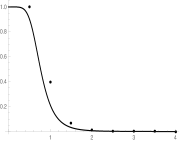
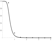
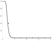
$P_{\rm BH}$             $\frac{\ell}{\ell_{D}}$
$D=4$                            $D=5$                            $D=8$                            $D=9$

Figure 2: Probability $P_{\rm BH}(\ell)$ of a particle, described by a Gaussian with $\ell=\lambda_{m}$, to be a black hole (dots) compared to its analytical approximation.

3.2 $(1+1)-$dimensional space-time

In $D=1$, from Eqs. (2.4) and (2.15), we have

$$P_{\rm S}(r<r_{\rm H})=\mathrm{erf}\left(\frac{r_{\rm H}}{\ell}\right)\ ,$$ (3.9)

and

$$\mathcal{P}_{\rm H}(r_{\rm H})=\frac{2/\ell}{\Gamma\left(-\frac{1}{2},\frac{m^{2}}{\Delta^{2}}\right)}\,\Theta(R_{1}-|r_{\rm H}|)\,\exp\left\{-\frac{\ell^{2}}{4\,r_{\rm H}^{2}}\right\}\ .$$ (3.10)

Consequently, the black hole probability is

$$P_{\rm BH}=\frac{4/\ell}{\Gamma\left(-\frac{1}{2},\frac{m^{2}}{\Delta^{2}}\right)}\int_{0}^{R_{1}}\mathrm{erf}\left(\frac{r_{\rm H}}{\ell}\right)\exp\left\{-\frac{\ell^{2}}{4\,r_{\rm H}^{2}}\right\}\,\mbox{${\rm d}$}r_{\rm H}\ .$$ (3.11)

We note that this formula can just be obtained from Eq. (3.8) by setting $D=1$ and taking the complementary integration domain. Fig. 3 shows this probability as a function of $\ell\geq\lambda_{m}$ for various masses.

$P_{\rm BH}$     $\ell/\ell_{1}$

Figure 3: Probability $P_{\rm BH}(\ell,m)$ for a particle to be a black hole in $D=1$, for $m=m_{1}$ (solid line), $m=3\,m_{1}/4$ (dashed line) and $m=m_{1}/2$ (dotted line).

An immediate feature that differentiates the $(1+1)$-dimensional case from the $(1+D)$-dimensional cases is the rate of increase of the probability for source mass less than the Planck scale $m_{1}$. In higher dimensions, the probability of forming a black hole with $m\geq m_{D}$ is quite high for $\ell\simeq\ell_{D}$, and drops significantly, at the same length scale, for $m<m_{D}$. For $D=1$, the drop is much slower and sources with $m<m_{1}$ have a comparably larger probability to be black holes. However, the main difference is that the maximum $P_{\rm BH}\simeq 0.45$, precisely obtained for $\ell=\lambda_{m}$, and does not depend on $m$. This is in agreement with the fact that, in $D=1$, the gravitational constant $G_{1}=1/\hbar$ and

$$\mbox{$\langle\,\hat{r}_{\rm H}\,\rangle$}\simeq R_{1}(m)\simeq\lambda_{m}\ ,$$ (3.12)

for any values of $m$.

This means the larger the mass $m$, the smaller the Compton length and the horizon radius (which would instead be larger in $D\geq 3$). Correspondingly, for a given width $\ell$, the probability the object is a black hole increases for decreasing mass (according to the fact that $\langle\,\hat{r}_{\rm H}\,\rangle$ becomes larger), and the source can never be a truly classical black hole (with $\mbox{$\langle\,\hat{r}_{\rm H}\,\rangle$}\gg\lambda_{m}$) in $D=1$.

This result is consistent with the notion that black holes in $(1+1)$-dimensional space-time are strictly quantum objects, as discussed in Ref. [26]. Furthermore, it can be understood to support several recent results suggesting the gravitational physics (and corresponding black holes) in the sub-Planckian regime is two dimensional [24, 25]. Said another way, black holes in the (sub-)Planckian regime will naturally form as effective $(1+1)$-dimensional objects, and in this sense the duality in mass-dependence between the $(1+3)$- and $(1+1)$-dimensional Schwarzschild metric is due to dimensional reduction.

4 GUP from HWF

We now derive the uncertainties in expectation values of quantities of relevance in this framework, and as a result derive the form of the GUP. Given the HWF (2.14), the expectation value of an operator $\hat{O}_{\rm H}$ is obtained from

$$\mbox{$\langle\,\hat{O}_{\rm H}\,\rangle$}=\Omega_{D-1}\int_{0}^{\infty}{\psi^{*}_{\rm H}(r_{\rm H})\,\hat{O}_{\rm H}\,\psi_{\rm H}(r_{\rm H})\,r_{\rm H}^{D-1}\,\mbox{${\rm d}$}r_{\rm H}}\ .$$ (4.1)

A straightforward example is given by

$$\mbox{$\langle\,\hat{r}_{\rm H}\,\rangle$}=\frac{\Gamma\left(\frac{D+1}{2D-4},\frac{m^{2}}{\Delta^{2}}\right)}{\Gamma\left(\frac{D}{2D-4},\frac{m^{2}}{\Delta^{2}}\right)}\,\left(\frac{\Delta}{m}\right)^{\frac{1}{D-2}}\,R_{D}\ .$$ (4.2)

By writing $\Gamma(s,x)=x^{s}\,\mathrm{E}_{1-s}(x)$, where $E_{n}$ is the generalised exponential integral

$$\mathrm{E}_{n}(x)\,=\,\int_{1}^{\infty}\frac{e^{-xt}}{t^{n}}\,\mbox{${\rm d}$}t\ ,$$ (4.3)

the above result reads

$$\mbox{$\langle\,\hat{r}_{\rm H}\,\rangle$}=\frac{\mathrm{E}_{\frac{D-5}{2D-4}}(\frac{m^{2}}{\Delta^{2}})}{\mathrm{E}_{\frac{D-4}{2D-4}}(\frac{m^{2}}{\Delta^{2}})}\,R_{D}\ .$$ (4.4)

We likewise obtain

$$\mbox{$\langle\,\hat{r}_{\rm H}^{2}\,\rangle$}=\frac{\mathrm{E}_{\frac{D-6}{2D-4}}(\frac{m^{2}}{\Delta^{2}})}{\mathrm{E}_{\frac{D-4}{2D-4}}(\frac{m^{2}}{\Delta^{2}})}\,R_{D}^{2}\ ,$$ (4.5)

and estimate the relative uncertainty in the horizon as

$$\Delta r_{\rm H}=\sqrt{\mbox{$\langle\,\hat{r}_{\rm H}^{2}\,\rangle$}-\mbox{$\langle\,\hat{r}_{\rm H}\,\rangle$}^{2}}=\sqrt{\frac{\mathrm{E}_{\frac{D-6}{2D-4}}(\frac{m^{2}}{\Delta^{2}})}{\mathrm{E}_{\frac{D-4}{2D-4}}(\frac{m^{2}}{\Delta^{2}})}-\left(\frac{\mathrm{E}_{\frac{D-5}{2D-4}}(\frac{m^{2}}{\Delta^{2}})}{\mathrm{E}_{\frac{D-4}{2D-4}}(\frac{m^{2}}{\Delta^{2}})}\right)^{2}}\,R_{D}\ .$$ (4.6)

Fig. 4 shows the plots of (4.4) and (4.6) for $D>3$ as functions of $\ell/\ell_{D}$, since

$$\frac{m}{\Delta}\,=\,\frac{\ell\,m}{\ell_{D}\,m_{D}}\,\varpropto\,\frac{\ell}{\ell_{D}}\ .$$ (4.7)

It is also trivial to see that, for $\ell\gg\ell_{D}$, we recover the expected classical results

$$\mbox{$\langle\,\hat{r}_{\rm H}\,\rangle$}\simeq R_{D}\ ,\qquad\Delta r_{\rm H}\simeq 0\ .$$ (4.8)

The above expressions (4.4) and (4.6) also hold in $D=1$, and are displayed in Fig. 5.

$\frac{\mbox{$\langle\,\hat{r}_{\rm H}\,\rangle$}}{R_{D}}$     $\ell/\ell_{D}$
$\frac{\Delta{r}_{\rm H}}{R_{D}}$     $\ell/\ell_{D}$
$D=4$                                                      $D=5$

Figure 4: Plots of $\langle\,\hat{r}_{\rm H}\,\rangle$ (upper panel) and $\Delta r_{\rm H}$ (lower panels) as functions of $\ell/\ell_{D}$, for $D=4$ (left) and $D=5$ (right), with $m=m_{D}$ (solid line), $m=\frac{3}{4}\,m_{D}$ (dashed line) and $m=\frac{1}{2}\,m_{D}$ (dotted line).

$\frac{\mbox{$\langle\,\hat{r}_{\rm H}\,\rangle$}}{R_{1}}$     $\frac{\Delta{r}_{\rm H}}{R_{1}}$ $\ell/\ell_{1}$

Figure 5: Plot of $\langle\,\hat{r}_{\rm H}\,\rangle$ and $\Delta r_{\rm H}$ as functions of $\ell$ for $D=1$.

The GUP follows by linearly combining the usual Heisenberg uncertainty with the uncertainty in the horizon size,

$$\Delta r=\Delta r_{\rm QM}+\alpha\,\Delta r_{\rm H}\ ,$$ (4.9)

where $\alpha$ is a dimensionless coefficient that one could try to set experimentally. We can compute the Heisenberg part starting from the state (2.4), that is

$$\mbox{$\langle\,\hat{r}^{n}\,\rangle$}=\Omega_{D-1}\int_{0}^{\infty}\tilde{\psi}^{*}(r)\,\hat{r}^{n}\,\tilde{\psi}(r)\,r^{D-1}\,\mbox{${\rm d}$}r=\frac{\Gamma\left(\frac{D+n}{2}\right)}{\Gamma\left(\frac{D}{2}\right)}\,\ell^{n}\ .$$ (4.10)

Using $\Gamma(z+1)=z\,\Gamma(z)$, this yields

$$\mbox{$\langle\,\hat{r}\,\rangle$}=\frac{2^{1-D}\sqrt{\pi}\,(D-1)!}{\Gamma\left(\frac{D}{2}\right)^{2}}\,\ell\ ,$$ (4.11)

and

$$\mbox{$\langle\,\hat{r}^{2}\,\rangle$}=\frac{D}{2}\,\ell^{2}\ ,$$ (4.12)

so that

$$\Delta r_{\rm QM}=\sqrt{\frac{D}{2}-\left(\frac{2^{1-D}\sqrt{\pi}}{\Gamma\left(\frac{D}{2}\right)^{2}}\,(D-1)!\right)^{2}}\,\ell=A_{D}\,\ell\ .$$ (4.13)

Using instead the state (2.5) in momentum space, the same procedure yields

$$\Delta p=A_{D}\,\Delta=A_{D}\,\frac{m_{D}\,\ell_{D}}{\ell}\ .$$ (4.14)

Expressing $\ell$ and $\Delta$ from the above equation as functions of $\Delta p$, we have

$$\frac{\Delta r}{\ell_{D}}\!\! = \!\!A_{D}^{2}\,\frac{m_{D}}{\Delta p}+\alpha\,\sqrt{\frac{\mathrm{E}_{\frac{D-6}{2D-4}}\left(\frac{A_{D}^{2}m^{2}}{(\Delta p)^{2}}\right)}{\mathrm{E}_{\frac{D-4}{2D-4}}\left(\frac{A_{D}^{2}m^{2}}{(\Delta p)^{2}}\right)}-\left[\frac{\mathrm{E}_{\frac{D-5}{2D-4}}\left(\frac{A_{D}^{2}m^{2}}{(\Delta p)^{2}}\right)}{\mathrm{E}_{\frac{D-4}{2D-4}}\left(\frac{A_{D}^{2}m^{2}}{(\Delta p)^{2}}\right)}\right]^{2}}\,\left(\frac{2}{|D-2|}\,\frac{m}{m_{D}}\right)^{\frac{1}{D-2}}\ ,$$ (4.15)

which is rather cumbersome. A straightforward simplification occurs by setting width of the wave-packet equal to the Compton length, $\ell=\lambda_{m}$, so that, from Eqs. (2.7) and (4.14),

$$m=\Delta=\frac{\Delta p}{A_{D}}$$ (4.16)

and the GUP then reads

$$\frac{\Delta r}{\ell_{D}}\!\! = \!\!A_{D}^{2}\frac{m_{D}}{\Delta p}+\alpha\,\sqrt{\frac{\mathrm{E}_{\frac{D-6}{2D-4}}(1)}{\mathrm{E}_{\frac{D-4}{2D-4}}(1)}-\left(\frac{\mathrm{E}_{\frac{D-5}{2D-4}}(1)}{\mathrm{E}_{\frac{D-4}{2D-4}}(1)}\right)^{2}}\left(\frac{2}{|D-2|}\,\frac{\Delta p}{A_{D}m_{D}}\right)^{\frac{1}{D-2}}$$ (4.17)

$$= \!\!\frac{C_{\rm QM}}{\Delta p}+C_{\rm H}\,\Delta p^{\frac{1}{D-2}}\ ,$$

where $C_{\rm QM}$ and $C_{\rm H}$ are constants (independent of $\Delta p$). Fig. 6 shows $\Delta r$ for different spatial dimensions, setting $\alpha=1$ for simplicity. In all the higher-dimensional cases, we obtain the same qualitative behaviour, with a minimum length uncertainty $L_{D}$

$$L_{D}=\ell_{D}\left(\frac{D-1}{D-2}\right)\,(2A_{D})^{\frac{1}{D-1}}\left(\alpha\sqrt{\frac{\mathrm{E}_{\frac{D-6}{2D-4}}(1)}{\mathrm{E}_{\frac{D-4}{2D-4}}(1)}-\left(\frac{\mathrm{E}_{\frac{D-5}{2D-4}}(1)}{\mathrm{E}_{\frac{D-4}{2D-4}}(1)}\right)^{2}}\right)^{\frac{D-2}{D-1}}$$ (4.18)

corresponding to an energy scale $M_{D}$, satisfying

$$M_{D}=m_{D}\,\frac{(D-2)}{2^{\frac{1}{D-1}}}\,\left[\alpha\sqrt{\frac{\mathrm{E}_{\frac{D-6}{2D-4}}(1)}{\mathrm{E}_{\frac{D-4}{2D-4}}(1)}-\left(\frac{\mathrm{E}_{\frac{D-5}{2D-4}}(1)}{\mathrm{E}_{\frac{D-4}{2D-4}}(1)}\right)^{2}}\right]^{\frac{2-D}{D-1}}\,A_{D}^{\frac{2D-3}{D-1}}\ .$$ (4.19)

The impact of $\alpha$ on this minimum length is then shown in Fig. 7, where we plot the scale $M_{D}$ corresponding to the minimum $L_{D}$ as a function of this parameter, and in Fig. 8, where we plot directly $L_{D}$. For all values of $D$ considered here, assuming $M_{D}\simeq m_{D}$ favours large values of $\alpha$, whereas requiring $L_{D}\simeq\ell_{D}$ would favour small values of $\alpha$.

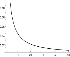
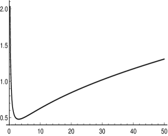
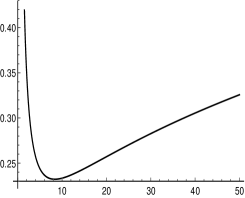
$\frac{\Delta r}{\ell_{D}}$         $\frac{\Delta p}{m_{D}}$
$D=1$                                     $D=4$                                     $D=5$

Figure 6: Plots of $\Delta r/\ell_{D}$ as function of $\Delta p/m_{D}$ for $D=1$, $4$ and $5$ and $\alpha=1$.

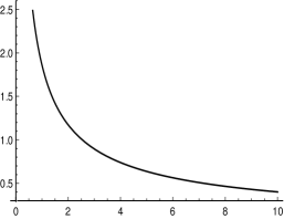
${\frac{M_{D}}{m_{D}}}$     $\alpha$
$D=4$                                     $D=5$

Figure 7: Minimum scale $M_{D}$ as function of the parameter $\alpha$ for $D=4$ and $5$.

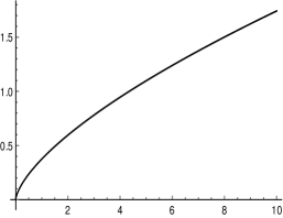
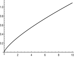
${\frac{L_{D}}{\ell_{D}}}$     $\alpha$
$D=4$                                     $D=5$

Figure 8: Minimum scale $L_{D}$ as function of the parameter $\alpha$ for $D=4$ and $5$.

If we now apply the above result (4.17) in $D=1$, we see that the complete expression is of the usual Heisenberg form,

$$\frac{\Delta r}{\ell_{1}} \!\!=\!\! A_{1}^{2}\,\frac{m_{1}}{\Delta p}+\frac{\alpha}{2}\sqrt{\frac{\mathrm{E}_{\frac{5}{2}}(1)}{\mathrm{E}_{\frac{3}{2}}(1)}-\left(\frac{\mathrm{E}_{2}(1)}{\mathrm{E}_{\frac{3}{2}}(1)}\right)^{2}}\,\frac{A_{1}m_{1}}{\Delta p}$$ (4.20)

$$\!\!=\!\! \frac{C_{\rm QM}+C_{\rm H}}{\Delta p}\ ,$$

and there is no minimum length for any mass-scale. This conclusion can also be inferred by the fact that Eqs. (4.18) and (4.19) are not well defined in $D=1$.

5 Conclusions

In this paper we extended the results of Refs. [6, 9] by embedding a massive source in a $(1+D)$-dimensional space-time. Shaping the wave packet with a Gaussian distribution, we computed its related horizon wave function and derived the probability $P_{\rm BH}$ that this massive source be inside its own horizon, which characterises a (quantum) black hole.

The higher-dimensional cases $D>3$ look qualitatively very similar to the standard $(3+1)$-scenario, with a probability $P_{\rm BH}$ of similar shape, and a related GUP leading to the existence of a minimum length scale. However, one of the main results is that the probability $P_{\rm BH}$ for fixed mass decreases for increasing $D>3$. In fact, for $m\simeq m_{D}$, one has $P_{\rm BH}\simeq 0.14$ for $D=5$, which further decreases to $P_{\rm BH}\simeq 3\times 10^{-3}$ for $D=9$. This implies that, although the fundamental scale $m_{D}$ could be smaller for larger $D$, one must still reach an energy scale significantly larger than $m_{D}$ in order to produce a black hole. It is clear that this should have a strong impact on the estimates of the number of black holes produced in colliders which are based on models with extra spatial dimensions, and, conversely, on the bounds on extra-dimensional parameters obtained from the lack of observation of these objects.

We also note that the parameters of the source have not been restricted to satisfy Buchdahl’s inequality [5], which is essentially the condition for a source not to be a black hole in classical general relativity. Since the HWF is explicitly devised to include quantum effects, such inequality cannot be assumed. We can however see that one indeed finds a large probability that the object is a black hole when Buchdahl’s inequality in $D=3$ is violated (that is, for $m\gtrsim m_{\rm p}$). For $D>3$, our conclusion can therefore be viewed as indicating a correction to Buchdahl’s inequality, since the ratio $m/m_{D}$ must be larger for larger $D$ in order to have a (significant probability to form a) black hole.

The effective $(1+1)$-dimensional scenario differs from the higher-dimensional models. In the latter case, the black hole probability increases as the energy of the system (i.e. the mass of the particle) grows above the relevant “gravitational energy scale” $m_{D}$. On the contrary, in $D=1$, black holes with masses far below $m_{1}$ are more likely, but the maximum probability never exceeds $P_{\rm BH}\simeq 0.5$ regardless of the mass. These features support the claim that two-dimensional black holes are purely quantum objects, and are particularly important for the sub-Planckian regime of lower dimensional theories, where an effective dimensional reduction is expected [26]. Moreover, the related GUP further supports the above arguments, since in $D=1$ there is no minimum length or mass.

We would like to conclude by remarking the fact that the present analysis does not consider the time evolution of the system, as the particle is taken at a fixed instant of time, which is therefore left for future extensions.

Acknowledgments

R. C. and A. G. are partly supported by INFN grant FLAG. R. T. C. is supported by CAPES and PDSE.  J. M. was supported by a Continuing Faculty Grant from the Frank R. Seaver College of Science and Engineering at LMU.

References

- [1] S. Hossenfelder, Living Rev. Rel. 16, 2 (2013); R. Casadio, O. Micu and P. Nicolini, Fundam. Theor. Phys. 178 (2015) 293.
- [2] C. J. Hogan and O. Kwon, “Statistical Measures of Planck Scale Signal Correlations in Interferometers,” arXiv:1506.06808 [gr-qc]; O. Kwon and C. J. Hogan, “Interferometric Probes of Planckian Quantum Geometry,” [arXiv:1410.8197 [gr-qc]]; S. Hossenfelder, Adv. High Energy Phys. 2014 (2014) 950672.
- [3] K. S. Thorne, in J.R. Klauder, Magic Without Magic, San Francisco 1972, 231-258.
- [4] V. V. Dodonov and S. S. Mizrahi, Phys. Lett. A. 177 (1993) 394.
- [5] H. A. Buchdahl, Phys. Rev. 116 (1959) 1027; H. Andréasson, J. Diff. Eqs. 245, 2243 (2008); H. Andréasson, Living Rev. Relativity 14, 4 (2011).
- [6] R. Casadio, “Localised particles and fuzzy horizons: A tool for probing Quantum Black Holes,” arXiv:1305.3195 [gr-qc].
- [7] R. Casadio and F. Scardigli, Eur. Phys. J. C 74 (2014) 2685.
- [8] R. Casadio, O. Micu and F. Scardigli, Phys. Lett. B 732 (2014) 105.
- [9] R. Casadio, “Horizons and non-local time evolution of quantum mechanical systems,” Eur. Phys. J. C 75 (2015) 160.
- [10] R. Casadio, O. Micu and D. Stojkovic, Phys. Lett. B 747 (2015) 68; JHEP 1505 (2015) 096.
- [11] G. Dvali and C. Gomez, JCAP 01, 023 (2014); “Black Hole’s Information Group”, arXiv:1307.7630; Eur. Phys. J. C 74, 2752 (2014); Phys. Lett. B 719, 419 (2013); Phys. Lett. B 716, 240 (2012); Fortsch. Phys. 61, 742 (2013); G. Dvali, C. Gomez and S. Mukhanov, “Black Hole Masses are Quantized,” arXiv:1106.5894 [hep-ph]; G. Dvali and C. Gomez, JCAP 1401, no. 01, 023 (2014); G. Dvali and C. Gomez, “Quantum Exclusion of Positive Cosmological Constant?,” arXiv:1412.8077 [hep-th].
- [12] R. Casadio, A. Giugno and A. Orlandi, “Thermal corpuscular black holes”, Phys. Rev. D 91, 124069 (2015).
- [13] F. Kuhnel, Phys. Rev. D 90, 084024 (2014); F. Kuhnel and B. Sundborg, “Modified Bose-Einstein Condensate Black Holes in d Dimensions,” arXiv:1401.6067 [hep-th]; F. Kuhnel and B. Sundborg, JHEP 1412, 016 (2014); F. Kuhnel and B. Sundborg, Phys. Rev. D 90, 064025 (2014).
- [14] W. Mück and G. Pozzo, JHEP 1405, 128 (2014).
- [15] S. Hofmann and T. Rug, “A Quantum Bound-State Description of Black Holes,” arXiv:1403.3224 [hep-th].
- [16] R. Casadio, A. Giugno, O. Micu and A. Orlandi, Phys. Rev. D 90, 084040 (2014); R. Casadio and A. Orlandi, JHEP 1308 (2013) 025.
- [17] A. Davidson and B. Yellin, Phys. Lett. B 736 267.
- [18] N. Arkani-Hamed, S. Dimopoulos and G. R. Dvali, Phys. Lett. B 429 (1998) 263; I. Antoniadis, N. Arkani-Hamed, S. Dimopoulos and G. R. Dvali, Phys. Lett. B 436 (1998) 257.
- [19] L. Randall and R. Sundrum, Phys. Rev. Lett. 83 (1999) 3370; Phys. Rev. Lett. 83 (1999) 4690.
- [20] R. Maartens and K. Koyama, Living Rev. Rel. 13 (2010) 5.
- [21] J. R. Mureika, “Primordial Black Hole Evaporation and Spontaneous Dimensional Reduction", Phys. Lett. B 716, 171 (2012).
- [22] R. Loll, Nucl. Phys. Proc. Suppl. 94, 96 (2001); J. Ambjorn, J. Jurkiewicz, R. Loll, Phys. Rev. D 72, 064014 (2005); “Quantum Gravity, or The Art of Building Spacetime,” in Approaches to Quantum Gravity, ed. D. Oriti, Cambridge University Press (2006).
- [23] L. Modesto and P. Nicolini, Phys. Rev. D 81, 104040 (2010).
- [24] P. Nicolini and E. Spallucci, Adv. High Energy Phys. 2014, 805684 (2014).
- [25] B. J. Carr, J. Mureika and P. Nicolini, JHEP 1507 (2015) 052.
- [26] J. Mureika and P. Nicolini, Eur. Phys. J. Plus 128, 78 (2013).
- [27] L. Anchordoqui, D. C. Dai, M. Fairbairn, G. Landsberg and D. Stojkovic, Mod. Phys. Lett. A 27, 1250021 (2012); L. A. Anchordoqui, D. C. Dai, H. Goldberg, G. Landsberg, G. Shaughnessy, D. Stojkovic and T. J. Weiler, Phys. Rev. D 83, 114046 (2011); D. Stojkovic, Rom. J. Phys. 57, 210 (2012).
- [28] J. R. Mureika and D. Stojkovic, Phys. Rev. Lett. 106, 101101 (2011); Phys. Rev. Lett. 107, 169002 (2011).
- [29] N. Afshordi and D. Stojkovic, Phys. Lett. B 739, 117 (2014).
- [30] D. Stojkovic, Mod. Phys. Lett. A 28, 1330034 (2013).
- [31] R. B. Mann, A. Shiekh, and L. Tarasov, Nucl. Phys. B 341, 134 (1990)
- [32] S. Dimopoulos and G. L. Landsberg, Phys. Rev. Lett. 87 (2001) 161602 [hep-ph/0106295].