On recursive algorithms for inverting tridiagonal matrices

Abstract

If $A$ is a tridiagonal matrix, then the equations $AX=I$ and $XA=I$ defining the inverse $X$ of $A$ are in fact the second order recurrence relations for the elements in each row and column of $X$. Thus, the recursive algorithms should be a natural and commonly used way for inverting tridiagonal matrices – but they are not. Even though a variety of such algorithms were proposed so far, none of them can be applied to numerically invert an arbitrary tridiagonal matrix. Moreover, some of the methods suffer a huge instability problem. In this paper, we investigate these problems very thoroughly. We locate and explain the different reasons the recursive algorithms for inverting such matrices fail to deliver satisfactory (or any) result, and then propose new formulae for the elements of $X=A^{-1}$ that allow to construct the asymptotically fastest possible algorithm for computing the inverse of an arbitrary tridiagonal matrix $A$, for which both residual errors, $\|AX-I\|$ and $\|XA-I\|$, are always very small.

1 Introduction

Matrix inversion has quite numerous applications in statistics, cryptography, computer graphics, etc. It is hard to imagine a computation system or a scientific programming environment without a library or a function that calculates the inverse of a matrix.

In many applications, where the inverse of a matrix appears, there is no actual need for direct computation of the inverse, as the corresponding problem can be solved by computing the solution of a matrix equation or, in particular cases, a system of linear equations. There are some problems, however, where the inverse of a matrix is indeed required.

Even though the problem of computing matrix inverse has been extensively studied and described in many numerical monographs, there is a variety of new papers dealing with the subject. In the last couple of years, a number of algorithms for inverting structured matrices (block, banded) were proposed. This paper focuses on recursive algorithms for inverting tridiagonal matrices.

The existing recursive algorithms for computing the inverse of this kind of matrices are not very popular and are not commonly used. This is mostly because there are wide classes of matrices for which these algorithms cannot be applied due to their instability or other kind of limitations (it will be described in more detail throughout the paper). In this paper, we analyse the reasons of these disadvantages and search for the way to eliminatethem. As a result, new formulae for the elements of the inverse of a tridiagonal matrix $A$ are proposed, which allow a very fast and accurate computation of $X=A^{-1}$, and can be applied to any non-singular tridiagonal matrix. To our knowledge, it is the only method that guarantees, in general, very small, both left and right, residual errors.

Let $A\in\mathbb{R}^{n\times n}$ be a tridiagonal matrix, i.e. a matrix whose elements satisfy $a_{ij}=0$ if $|i-j|>1$ ($i,j=1,2,\dots,n$). The most common algorithms for evaluating $A^{-1}$ are based on solving the matrix equation $AX=I$ (or $XA=I$; throughout the paper, by $X$, we shall denote the numerically computed inverse of a tridiagonal matrix $A$, or the inverse which is to be computed, and by $I$, the identity matrix). If the above equation is solved using, for example, Gaussian elimination with partial pivoting or using orthogonal transformations (e.g., Givens rotations), the computed inverse satisfies (c.f. [3, § 6.12])

$$\|AX-I\hskip 0.86108pt\|\,\leq\,\varepsilon\hskip 0.43057ptK\hskip 0.43057pt\mathrm{cond}(A),$$

where $\varepsilon$ is the machine precision, $K$ is a small constant, and $\mathrm{cond}(A)$ is the condition number of $A$. In such a case, it is easy to verify that the relative error $\|A^{-1}\|^{-1}\|X-A^{-1}\|$ satisfies a similar bound:

$$\frac{\|X-A^{-1}\|}{\|A^{-1}\|}\leq\,\|AX-I\hskip 0.86108pt\|\,\leq\,\varepsilon\hskip 0.43057ptK\hskip 0.43057pt\mathrm{cond}(A).$$

However, the bound is not so favourable in the case of the second residual error. We have, as $X=A^{-1}AX=A^{-1}\big{(}I+AX-I\big{)}$,

$$\|XA-I\hskip 0.86108pt\| =\,\|A^{-1}\big{(}I+AX-I\big{)}A-I\hskip 0.43057pt\|$$

$$=\,\|A^{-1}\big{(}AX-I\big{)}A\|\,\leq\,\mathrm{cond}(A)\|AX-I\hskip 0.43057pt\|\,\leq\,\varepsilon\hskip 0.43057ptK\hskip 0.43057pt\mathrm{cond}(A)^{2}.$$

Indeed, consider the following tridiagonal matrix $A\in\mathbb{R}^{10\times 10}$ whose elements $a_{ij}$ for $i,j\in\{1,2,\dots,10\hskip 0.86108pt\}$, $|i-j|\leq 1$ are listed column-wise in the following table:

$$\begin{bmatrix}&0&1/83&1/70&1/65&1/49&16&49&57&70\,\\ 1&1/98&1/84&1/53&92&55&86&1/84&1/49&83\,\\ \hskip 0.86108pt79&61&18&3&1/32&1/37&1/45&0&0&\end{bmatrix}\hskip 0.43057pt.$$

The condition number $\mathrm{cond}_{2}(A)\simeq 6.1\cdot 10^{8}$. If the inverse $X$ is computed in the double precision arithmetic ($\varepsilon=2^{-52}\simeq 2.2\cdot 10^{-16}$) using the Matlab command X =  A\eye(10), i.e. using the Gaussian elimination with partial pivoting, then we will obtain the result that satisfies

$$\|AX-I\hskip 0.43057pt\|_{2}\,\simeq\,5.8\cdot 10^{-9}\,\simeq\,\varepsilon\hskip 0.43057pt0.043\,\mathrm{cond}_{2}(A).$$

For the left residual error, however, we have

$$\|XA-I\hskip 0.43057pt\|_{2}\,\simeq\,\textbf{3.\hskip 0.43057pt4}\,\simeq\,5.8\cdot 10^{8}\hskip 0.86108pt\|AX-I\hskip 0.43057pt\|_{2}\,\simeq\,0.95\hskip 0.86108pt\mathrm{cond}_{2}(A)\|AX-I\hskip 0.43057pt\|_{2},$$

and there are elements larger than $3$ outside the main diagonal in the matrix $XA$. Such an inverse may not always be considered as a very satisfactory one. This problem has been already considered by Higham in [4] and [10, § 13.3], who proposed a symmetric algorithm for computing $A^{-1}$ based on $LU$ factorisation. However, as the algorithm uses no pivoting strategy, it is not stable in general.

The asymptotic complexity of the most common algorithms for inverting tridiagonal matrices equals: $3n^{2}+O(n)$ in the case of Gaussian elimination without pivoting, $5n^{2}+O(n)$ in the case of Gaussian elimination with partial pivoting, and $7.5n^{2}+O(n)$ in the case of the algorithm based on Givens rotations. In the present paper, we will propose some new formulae which allow to construct a stable, always applicable algorithm with the smallest possible asymptotic complexity: $n^{2}+O(n)$. The authors do not know the formal proof of stability of the algorithm yet, but strong justification is given to support the conjecture that the inverse $X$ of a tridiagonal matrix $A\in\mathbb{R}^{n\times n}$ computed using the proposed method satisfies

$$\max\big{\{}\|AX-I\hskip 0.43057pt\|,\|XA-I\hskip 0.43057pt\|\big{\}}\,\leq\,\varepsilon\hskip 0.43057ptK(n)\hskip 0.43057pt\mathrm{cond}(A),$$

where $K(n)=O(n)$.

In the incoming section, we shall present a short review of the recursive approach to the problem of inverting a tridiagonal matrix. We shall also recall the basic facts from the theory of difference equations that will help to explain the reasons several recently proposed recursive algorithms for inverting tridiagonal matrices fail (or are unstable) for some important classes of matrices.

In Section 3, we present a new efficient method, also based on some recursions, which can be successfully applied to invert any non-singular tridiagonal matrix.

2 A short review of the recursive algorithms and the theory of the second order difference equations

In this section, we review several algorithms for recursive computation of the inverse of a tridiagonal matrix. Showing the strong and the weak sides of these algorithms will lead us to the main result of the paper.

2.1 The naive recursion

It is well known that for $B\in\mathbb{R}^{n\times n}$ and  $c\in\mathbb{R}^{n}$ the product $Bc$ can be interpreted as the linear combination of columns of the matrix $B$,

$$Bc=\sum\limits_{k=1}^{n}c_{k}B_{k}\,,$$

where $B_{k}$ denotes the $k$-th column of $B$. Such interpretation is very convenient if $c$ has only a few non-zero elements.

Let $A\in\mathbb{R}^{n\times n}$ be a tridiagonal matrix ($a_{ij}=0$ if $|i-j|>1$). Then, the equation $XA=I$ implies the following relations:

$$a_{k-1,k}X_{k-1}+a_{k,k}X_{k}+a_{k+1,k}X_{k+1} =I_{k}\quad(1<k<n)\,,$$

$$a_{n-1,n}X_{n-1}+a_{n,n}X_{n} =I_{n}\,.$$

Thus, if we know the last column $X_{n}$ of $X$, then we can easily recursively compute the whole inverse matrix $X$:

$$\left.\begin{array}[]{l}\vspace{-6ex}\\ \displaystyle{X_{n-1}}\,=\,\,I_{n}\,-\,\frac{a_{n,n}}{a_{n-1,n}}X_{n}\,,\\ \hskip 0.43057pt\displaystyle{X_{k-1}}\,=\,\,I_{k}\,-\,\frac{a_{k,k}}{a_{k-1,k}}X_{k}\,-\,\frac{a_{k+1,k}}{a_{k-1,k}}X_{k+1}\quad(n>k>1)\,,\end{array}\quad\right\}$$ (2.1)

where we assume that $a_{k-1,k}\neq 0$ ($1<k\leq n$).

The above simple observation laid the basis of two recent algorithms, [6] and [9], for inverting tridiagonal matrices. In [6], the last column $X_{n}$ is computed using the LU factorisation without pivoting, while in [9], the Miller algorithm — a classical algorithm for computing the minimal solutions of second order difference equations — has been rediscovered.

Let us test the stability of the above scheme for a very small and very well conditioned matrix

$$A\,\,=\,\,\begin{pmatrix}\hskip 2.15277pt2016&1&&&&\\ \hskip 2.15277pt1&2016&1&&&\\ &1&2016&1&&\\ &&1&2016&1&\\ &&&1&2016&1\hskip 4.30554pt\\ &&&&1&2016\hskip 4.30554pt\\ \end{pmatrix}.\vspace{0.5ex}$$ (2.2)

For the inverse matrix $X$ computed in the double precision arithmetic using the algorithm [6] or [9] (the result does not depend on which of the above ways the last column of $X$ is calculated), we have

$$\|AX-I\hskip 0.43057pt\|_{2}\,\simeq\,\|XA-I\hskip 0.43057pt\|_{2}\,\simeq\,\textbf{4.4},$$

while $\mathrm{cond}_{2}(A)=1.002$. If the inverse is evaluated in Matlab: X =  A\eye(6), the residual errors satisfy $\|AX-I\hskip 0.43057pt\|_{2}\simeq\|XA-I\hskip 0.43057pt\|_{2}\simeq\varepsilon\simeq 2.2\cdot 10^{-16}$. The explanation of such a huge instability of the simple recursive algorithms based on (2.1) is quite simple if we recall some basic facts of the theory of linear second order difference equations (see, for example, [8] or [13]).

The three term (second order) homogenous recurrence (difference) equation can be written in general form as follows:

$$a_{-1}(k)\hskip 0.43057ptx_{k-1}\,+\,a_{0}(k)\hskip 0.43057ptx_{k}\,+\,a_{1}(k)\hskip 0.43057ptx_{k+1}\,=\,0\qquad(k>1,\,\,a_{\pm 1}(k)\neq 0),$$ (2.3)

where $a_{j}(k)$ ($j=-1,0,1$) are known coefficients, and $\{x_{k}\}_{k=1}^{\infty}$ is a solution we are looking for. The equation (2.3) has two-dimensional space of solutions. If there exist two linearly independent solutions $\{u_{k}\}$ and $\{y_{k}\}$ such that

$$\lim\limits_{k\to\infty}\frac{u_{k}}{y_{k}}\,=\,0\,,$$

then $\{u_{k}\}$ is called a minimal, and $\{y_{k}\}$ is called a dominant  solution. The forward recursion algorithm,

$$x_{k+1}=-a_{1}(k)^{-1}\big{(}a_{0}(k)\,x_{k}+a_{-1}(k)\,x_{k-1}\big{)}\hskip 0.43057pt,$$

is stable for dominant solutions only, while the backward recursion,

$$x_{k-1}=-a_{-1}(k)^{-1}\big{(}a_{0}(k)\,x_{k}+a_{1}(k)\,x_{k+1}\big{)}\hskip 0.43057pt,$$

is stable only for minimal solutions (at the present point, we do not consider the problem of obtaining the initial values for the above recurrences). If  for any pair $\{u_{k}\}$, $\{y_{k}\}$ of independent solutions we have

$$\liminf\limits_{k\to\infty}\frac{u_{k}}{y_{k}}\,=\,w>0\,,\qquad\limsup\limits_{k\to\infty}\frac{u_{k}}{y_{k}}\,=\,\mathcal{W}<\infty\,,$$

where $w,\,\mathcal{W}^{-1}\gg\varepsilon$, then both forward and backward recursion algorithms are stable (in the asymptotic sense).

In practice, we are usually interested in computing only a part of a solution of the recurrence equation (2.3), i.e. the values of $x_{k}$ for $1\leq k\leq n$ for some $n>0$. Note that the starting point ($k=1$) and the main (forward) direction of the recursion ($k=2,3,\dots$) is only a convention.

The space of all minimal solutions of the linear second order difference equation is one-dimensional. An important property of the minimal solutions and the algorithm for computing the values of such a solution is given in the following theorem.

Theorem 1 (Miller).

Assume that a three term recurrence equation (2.3) has a minimal solution $\{u_{k}\}$ which satisfies a normalising condition

$$\sum_{k=1}^{M}c_{k}u_{k}=S\neq 0\qquad(S,c_{k}\in\mathbb{R},\,\,\,0<M<\infty).$$

For $\hskip 0.43057ptn>1\hskip 0.43057pt$, define the values $x^{[n]}_{k}$ ($1\leq k\leq n+1$) as follows:

$$x^{[n]}_{n+1}=0,\quad x^{[n]}_{n}=d\neq 0,$$

$$x^{[n]}_{k-1}=-a_{-1}(k)^{-1}\big{(}a_{0}(k)\,x^{[n]}_{k}+a_{1}(k)\,x^{[n]}_{k+1}\big{)}\qquad(n\geq k>1)\hskip 0.43057pt.\vspace{0.75ex}$$

Then, for each $k\geq 1$

$$\quad\lim\limits_{n\to\infty}S_{n}^{-1}Sx^{[n]}_{k}=\,\hskip 0.86108ptu_{k}\hskip 0.43057pt,$$

where

$$S_{n}=\sum\limits_{k=0}^{M}c_{k}x^{[n]}_{k}\vspace{-0.5ex}$$

(we assume that $x^{[n]}_{k}=0$ if $k>n$).

Proof.

See [12] or [13, § 4]. ∎

Let us consider again the recursion (2.1), but only for the elements of the first row of the inverse matrix $X$. We may of course write that $x_{1,n+1}=0$. Additionally, if $a_{k-1,k}\neq 0$ for all $1<k\leq n$, then, theoretically, $x_{1,n}\neq 0$ (this will be justified in the later part of the paper; see also [11]). Consequently, we have

$$\begin{array}[]{l}x_{1,n+1}\hskip 0.43057pt=\hskip 0.43057pt0,\quad x_{1,n}\hskip 0.43057pt\neq\hskip 0.43057pt0,\\ \hskip 0.43057ptx_{1,k-1}\hskip 0.43057pt=\hskip 0.43057pt-{a_{k-1,k}^{-1}}{\big{(}a_{k,k}\hskip 0.43057ptx_{1,k}+a_{k+1,k}\hskip 0.43057ptx_{1,k+1}\big{)}}\qquad(n\geq k>1)\end{array}$$ (2.4)

and (also from the equation $XA=I$ ) $a_{1,1}x_{1,1}+a_{2,1}x_{1,2}=1\neq 0$. Comparing the above formulae to the ones of Theorem 1, we may conclude that if the recurrence equation for the first row of the inverse matrix $X$ has minimal and dominant solutions, then the elements $x_{1,1},x_{1,2},\dots,x_{1,n}$ of the first row of $X$ behave more like a minimal solution than like a dominant one. Therefore, the recursion (2.1) which is the backward recursion for $x_{1,k}$ ($n\geq k\geq 1$) is stable for all elements of the first row of the matrix $X$. In the case of the $s$-th row, we have

$$\begin{array}[]{l}x_{s,n+1}\hskip 0.43057pt=\hskip 0.43057pt0\hskip 0.43057pt,\qquad x_{s,k-1}\hskip 0.43057pt=\hskip 0.43057pt-{a_{k-1,k}^{-1}}{\big{(}a_{k,k}\hskip 0.43057ptx_{s,k}+a_{k+1,k}\hskip 0.43057ptx_{s,k+1}\big{)}}\qquad(n\geq k>s).\end{array}$$

Note that this recurrence is exactly the same as the recurrence (2.4), only the starting value $x_{1,n}$ is replaced by $x_{s,n}$. This implies that the recursion (2.1) is stable for all elements in the upper triangle of $X$. In the lower triangle of $X$, the situation is reversed. The recursion (2.1) is the forward recursion algorithm for the elements $x_{s,k}$ ($s>k\geq 1$, $s>1$), and therefore may be unstable if the corresponding recurrence equation,

$$a_{k+1,k}\hskip 0.43057ptx_{s,k+1}+a_{k,k}\hskip 0.43057ptx_{s,k}+a_{k-1,k}\hskip 0.43057ptx_{s,k-1}=0\qquad(s>k\geq 2),$$

has minimal and dominant solutions. Indeed, in the case of the matrix $X$ computed using (2.1), where $A$ is given by (2.2), we have

$$|X-A^{-1}|\,\,\simeq\,\,\|A^{-1}\|\begin{pmatrix}\hskip 0.86108pt\underline{6\cdot 10^{-16}}&2\cdot 10^{-19}&1\cdot 10^{-22}&1\cdot 10^{-25}&6\cdot 10^{-29}&3\cdot 10^{-32}\,\\ \hskip 0.86108pt6\cdot 10^{-13}&\underline{4\cdot 10^{-16}}&3\cdot 10^{-19}&1\cdot 10^{-22}&1\cdot 10^{-25}&6\cdot 10^{-29}\,\\ \hskip 0.86108pt1\cdot 10^{-09}&8\cdot 10^{-13}&\underline{6\cdot 10^{-16}}&3\cdot 10^{-19}&2\cdot 10^{-22}&1\cdot 10^{-25}\,\\ \hskip 0.86108pt1\cdot 10^{-06}&8\cdot 10^{-10}&4\cdot 10^{-13}&\underline{4\cdot 10^{-16}}&2\cdot 10^{-19}&1\cdot 10^{-22}\,\\ \hskip 0.86108pt2\cdot 10^{-03}&1\cdot 10^{-06}&4\cdot 10^{-10}&2\cdot 10^{-13}&\underline{2\cdot 10^{-16}}&2\cdot 10^{-19}\,\\ \hskip 0.86108pt4\cdot 10^{+00}&2\cdot 10^{-03}&1\cdot 10^{-06}&5\cdot 10^{-10}&2\cdot 10^{-13}&\underline{2\cdot 10^{-16}}\,\end{pmatrix}$$

(for readability, diagonal elements are underlined).

The recursion (2.1) was obtained from the matrix equation $XA=I$. The second, twin equation, $AX=I$, implies the analogous recurrence for rows of the matrix $X$. From the discussion above, the important result follows.

Corollary 1.

If the elements of the inverse $X$ of a tridiagonal matrix are computed recursively, then, in general, the algorithm is stable only if the recurrences are carried out towards the main diagonal of $X$.

We end this subsection by formulating the algorithm for stable recursive computation of the last column of $X$ (the algorithm is a consequence of Theorem 1 and the equation $AX_{n}=I_{n}$, and is a particular case of the Miller backward recursion algorithm):

$$y_{0} =\hskip 0.43057pt0,\quad y_{1}\hskip 0.43057pt=\hskip 0.43057pt1$$

$$y_{k+1} =\hskip 0.43057pt-a_{k,k+1}^{-1}\big{(}a_{k,k-1}\hskip 0.43057pty_{k-1}+a_{k,k}\hskip 0.43057pty_{k}\big{)}\quad\,(1\leq k<n),$$

$$x_{k,n} =\hskip 0.43057ptfy_{k}\quad\,(1\leq k\leq n),$$

where the normalising factor $f=\big{(}a_{n,n-1}y_{n-1}+a_{n,n}y_{n}\big{)}^{-1}$.

2.2 Two-way recursion

By Corollary 1, we conclude that a single recursion, like (2.1), cannot lead to a stable algorithm for inverting tridiagonal matrices. However, as the algorithm (2.1) computes the upper triangle of the inverse matrix $X$ correctly, we may use a similar scheme to compute the elements in the lower triangle, namely, compute the first column $X_{1}$ using the Miller algorithm, and then compute recursively the elements below the diagonal in the consecutive columns $X_{k}$ ($k=2,3,\dots,n-1$). The scheme looks as follows: compute the columns $X_{1}$ and $X_{n}$ using the Miller algorithm, and then set

$$\left.\begin{array}[]{rl}\vspace*{-7ex}\hfil\\ \displaystyle\big{\{}x_{s,n-1}\big{\}}_{s\hskip 0.3014pt=\hskip 0.3014pt1}^{n-1}&=\hskip 0.86108pt\displaystyle-\,\frac{a_{n,n}}{a_{n-1,n}}\,\big{\{}x_{s,n}\big{\}}_{s\hskip 0.3014pt=\hskip 0.3014pt1}^{\hskip 0.3014ptn-1}\hskip 0.43057pt,\\ \displaystyle\big{\{}x_{s,k-1}\big{\}}_{s\hskip 0.3014pt=\hskip 0.3014pt1}^{\hskip 0.3014ptk-1}&=\hskip 0.86108pt\displaystyle-\,\frac{a_{k,k}}{a_{k-1,k}}\,\big{\{}x_{s,k}\big{\}}_{s\hskip 0.3014pt=\hskip 0.3014pt1}^{\hskip 0.3014ptk-1}\hskip 0.86108pt-\,\frac{a_{k+1,k}}{a_{k-1,k}}\,\big{\{}x_{s,k+1}\big{\}}_{s\hskip 0.3014pt=\hskip 0.3014pt1}^{\hskip 0.3014ptk-1}\quad(n>k>2)\hskip 0.43057pt,\\ \displaystyle\big{\{}x_{s,2}\big{\}}_{s\hskip 0.3014pt=\hskip 0.3014pt3}^{n}&=\hskip 0.86108pt\displaystyle-\,\frac{a_{1,1}}{a_{2,1}}\,\big{\{}x_{s,1}\big{\}}_{s\hskip 0.3014pt=\hskip 0.3014pt3}^{n}\hskip 0.43057pt,\\ \displaystyle\big{\{}x_{s,k+1}\big{\}}_{s\hskip 0.3014pt=\hskip 0.3014ptk+2}^{n}&=\hskip 0.86108pt\displaystyle-\,\frac{a_{k,k}}{a_{k+1,k}}\,\big{\{}x_{s,k}\big{\}}_{s\hskip 0.3014pt=\hskip 0.3014ptk+2}^{n}\hskip 0.86108pt-\,\frac{a_{k-1,k}}{a_{k+1,k}}\,\big{\{}x_{s,k-1}\big{\}}_{s\hskip 0.3014pt=\hskip 0.3014ptk+2}^{n}\quad(1<k<n-1)\hskip 0.43057pt.\end{array}\right\}\vspace{0.25ex}$$ (2.5)

We assume that $a_{k-1,k}\neq 0$ and $a_{k,k-1}\neq 0$ for $1<k\leq n$. The above algorithm appears to be presented in print for the first time, but it is still not a very good one as we shall justify below.

Observe that the formulae (2.5) are based on the equations

$$a_{k-1,k}\hskip 0.43057ptx_{s,k-1}+a_{k,k}\hskip 0.43057ptx_{s,k}+a_{k+1,k}\hskip 0.43057ptx_{s,k+1}=0\quad\,\,(1\leq s\leq n,\,\,1\leq k\leq n,\,\,k\neq s)$$ (2.6)

(throughout the paper we assume than $a_{ij}=0$ and $x_{ij}=0$ if $i<1$, or $i>n$, or $j<1$, or $j>n$), while the Miller algorithm for computing the columns $X_{1}$ and $X_{n}$ is based on the equations

$$a_{k,k+1}\hskip 0.43057ptx_{k+1,j}+a_{k,k}\hskip 0.43057ptx_{k,j}+a_{k,k-1}\hskip 0.43057ptx_{k-1,j}=0\quad\,\,(1\leq j\leq n,\,\,1\leq k\leq n,\,\,k\neq j).$$ (2.7)

Theoretically, in our applications of the Miller algorithm we use the above equations only for $j\in\{1,n\}$. However, as $k\neq j$, all the equations (2.7) for $1\leq j<n$ and $k>j$ are in fact the same recurrence equations (an analogous observation is true for $n\geq j>1$ and $k<j$). The normalising factors used for computing the columns $X_{1}$ and $X_{n}$ by the Miller algorithm are derived from the two additional equations,

$$a_{1,1}\hskip 0.43057ptx_{1,1}+a_{1,2}\hskip 0.43057ptx_{2,1}=1\quad\mathrm{and}\quad a_{n,n-1}\hskip 0.43057ptx_{n-1,n}+a_{n,n}\hskip 0.43057ptx_{n,n}=1.$$

But the remaining equations,

$$\left.\begin{array}[]{l}a_{k-1,k}x_{k,k-1}+a_{k,k}x_{k,k}+a_{k+1,k}x_{k,k+1}=1,\\ a_{k,k+1}x_{k+1,k}+a_{k,k}x_{k,k}+a_{k,k-1}x_{k-1,k}=1,\end{array}\quad\right\}$$ (2.8)

for $1<k<n$, are nowhere used in the above algorithm. In other words, the presented two-way recursion algorithm computes the matrix $X$ which satisfy the following system of matrix equations

$$XA=D,\qquad A\hskip 0.43057ptX=H,$$

where $D$ and $H$ are diagonal matrices for which we only know that $h_{1,1}=h_{n,n}=1$. An interesting question arises: does the algorithm based on (2.5) computes the actual inverse of a tridiagonal matrix $A$, assuming that the computations are exact? The answer to the above question is delivered by the following theorem.

Theorem 2.

Let $A\in\mathbb{R}^{n\times n}$ be a non-singular tridiagonal matrix such that $a_{k,k-1}\neq 0$ and $a_{k-1,k}\neq 0$ for $1<k\leq n$. If a matrix $X$ is a solution of the system of matrix equations

$$XA=D,\qquad A\hskip 0.43057ptX=H,$$ (2.9)

where $D$ and $H$ are diagonal matrices and $H$ satisfy $h_{1,1}=h_{n,n}=1$, then $D=H=I$ and, consequently, $X=A^{-1}$.

Proof.

The equations (2.9) imply that

$$AD=A\hskip 0.43057ptXA=HA.$$

Equating the corresponding elements of the matrices $AD$ and $HA$ in a proper order, and recalling that $h_{1,1}=1$ and $a_{i,j}\neq 0$ for $|i-j|=1$, we obtain, in sequence,

$$1\,=\,h_{1,1}\,=\,d_{2,2}\,=\,h_{3,3}\,=\,d_{4,4}\,=\,h_{5,5}\,=\,\dots\,.$$ (2.10)

Similarly, but using the condition $h_{n,n}=1$, we get

$$1\,=\,h_{n,n}\,=\,d_{n-1,n-1}\,=\,h_{n-2,n-2}\,=\,d_{n-3,n-3}\,=\,h_{n-4,n-4}\,=\,\dots\,.$$ (2.11)

If $n$ is even, then from (2.10) and (2.11) we immediately obtain that $d_{i,i}=h_{i,i}=1$ for $1\leq i\leq n$. If $n$ is odd, then at least one of the diagonal elements of $A$ is different from 0 (otherwise there would be $\det(A)=0$). For simplicity, assume that $a_{1,1}\neq 0$. Then,

$$1\,=\,h_{1,1}\,=\,d_{1,1}\,=\,h_{2,2}\,=\,d_{3,3}\,=\,h_{4,4}\,=\,\dots\,.$$

By combining the above result with (2.10), again, we get $d_{i,i}=h_{i,i}=1$ for $1\leq i\leq n$. ∎

The above theorem implies that in theory, the algorithm based on the recursions (2.5) computes the correct inverse $X$ of a tridiagonal matrix $A$ with non-zero elements on the sub- and super- diagonals. The situation is a little different in practice. The numerical performance of this algorithm is far from perfection. As the lower and the upper triangles of $X$ are computed completely independently, the values of magnitude close to $\varepsilon\hskip 0.86108pt\mathrm{cond}(A)^{2}$ may appear along the main diagonals of the residual matrices $|AX-I|$ and $|XA-I|$. Thus, the search for a better algorithm has to be continued. Before it is done, we shall consider for a moment the complexity of the methods presented so far.

It is readily seen that the algorithm based on (2.5), like the one based on (2.1), has the complexity equal to $3n^{2}+O(n)$. However, if we take a closer look on the equations in (2.5), we can see that the recurrence for the elements in the upper triangle of $X$ (the first two lines) is exactly the same for each value of the row index $s$, only the initial values are different. Thus, we may carry out the recurrence only once, and then scale the result according to the corresponding initial values:

$$\left.\begin{array}[]{rl}\vspace*{-6.5ex}\hfil\\ \displaystyle\hat{z}_{n-1}&=\,\displaystyle-\,\frac{a_{n,n}}{a_{n-1,n}}\hskip 0.43057pt\hskip 0.43057pt1\hskip 0.43057pt,\\ \displaystyle\hat{z}_{k-1}&=\,\displaystyle-\,\frac{a_{k,k}}{a_{k-1,k}}\hskip 0.43057pt\hat{z}_{k}\,+\,\frac{a_{k+1,k}}{a_{k-1,k}}\hskip 0.43057pt\hat{z}_{k+1}\qquad(n>k>2)\hskip 0.43057pt,\\ \displaystyle\big{\{}x_{s,k-1}\big{\}}_{s\,=\,1}^{k-1}&=\,\hat{z}_{k-1}\big{\{}x_{s,n}\big{\}}_{s\,=\,1}^{k-1}\qquad(n\geq k>2)\hskip 0.43057pt.\end{array}\quad\right\}$$ (2.12)

The above scheme uses $\frac{1}{2}n^{2}+O(n)$ arithmetic operations. If a similar modification is done for the computation of the lower triangle of $X$, the complexity of the whole algorithm will drop to the smallest possible — as the inverse of a tridiagonal matrix has, in general, $n^{2}$ different elements — asymptotic value: $n^{2}+O(n)$.

2.3 The Lewis algorithm

In order to improve the numerical properties of the recursive algorithm for inverting tridiagonal matrices, we should include the known dependence between the elements in the upper triangle of the inverse matrix $X$ and the elements in the lower triangle. The simple formula that relates these elements was given in [11].

Lemma 1 (Lewis).

If $A\in\mathbb{R}^{n\times n}$ is a tridiagonal matrix such that $a_{k,k+1}\neq 0$ for $k=1,2,\dots,n-1$, and $X=A^{-1}$, then

$$x_{k+j,k}\,=\,\Bigg{(}\prod_{i=k}^{k+j-1}\frac{a_{i+1,i}}{a_{i,i+1}}\Bigg{)}x_{k,k+j}\qquad(1\leq k<n,\,\,1\leq j\leq n-k)\hskip 0.43057pt.$$ (2.13)

Proof.

See [11]. ∎

The formula (2.13) is a direct consequence (cf. [11]) of the equations

$$\sum_{i=-1}^{1}a_{k+i,k}\hskip 0.43057ptx_{k,k+i}\,=\,\sum_{i=-1}^{1}a_{k,k-i}\hskip 0.43057ptx_{k-i,k}\,=\,1\qquad(1\leq k\leq n),$$ (2.14)

i.e. is implied, in particular, by the equations (2.8) that were not used in the algorithm presented in the previous subsection. Now, the following algorithm with a very favourable numerical properties can be formulated: compute the last column $X_{n}$ using the Miller algorithm; compute the remaining elements in the upper triangle of $X$ using (2.12) for $k>1$, instead of for $k>2$; compute the lower triangle of $X$ using (2.13). This algorithm works very well if the two following conditions are satisfied: if $a_{k-1,k}\neq 0$ for all $2\leq k\leq n$, and if the values $\hat{z}_{k}$ ($n>k\geq 1$) in (2.12) do not grow too large, causing floating-point overflow (which is, unfortunately, a quite frequent case). A very similar algorithm was formulated in [11], where only the last column $X_{n}$ is computed in a slightly different (but mathematically and numerically equivalent) way.

Note that due to (2.13), the complexity of the above scheme grew to $\frac{3}{2}n^{2}+O(n)$. The complexity, however, can be reduced back to $n^{2}+O(n)$ if we apply the relation (2.13) in a little different way. The following theorem is one of the main results of [11]:

Theorem 3 (Lewis).

Assume that $A$ is a non-singular tridiagonal matrix which satisfies $a_{k-1,k}\neq 0$ and $a_{k,k-1}\neq 0$ for $2\leq k\leq n$. Let the sequences $\{\hat{z}_{k}\}$, $\{z_{k}\}$, $\{e_{k}\}$ be defined in the following way:

$$\left.\begin{array}[]{l}\vspace*{-7.25ex}\\ \displaystyle\hat{z}_{n}\hskip 0.43057pt=\,\hskip 0.43057pt1,\quad\displaystyle\hat{z}_{n-1}\hskip 0.43057pt=\,-\,\frac{a_{n,n}}{a_{n-1,n}},\quad\displaystyle\hat{z}_{k-1}\hskip 0.43057pt=\,-\,\frac{a_{k,k}}{a_{k-1,k}}\hat{z}_{k}\,-\,\frac{a_{k+1,k}}{a_{k-1,k}}\hat{z}_{k+1}\quad(n>k>1),\\ \displaystyle z_{1}\hskip 0.43057pt=\,\hskip 0.43057pt1,\quad\displaystyle z_{2}\hskip 0.43057pt=\,-\,\frac{a_{1,1}}{a_{2,1}}\hskip 0.43057pt,\quad\displaystyle z_{k+1}\hskip 0.43057pt=\,-\,\frac{a_{k,k}}{a_{k+1,k}}z_{k}\,-\,\frac{a_{k-1,k}}{a_{k+1,k}}z_{k-1}\quad(1<k<n),\\ \displaystyle e_{1}\hskip 0.43057pt=\,\hskip 0.43057pt1,\quad\displaystyle e_{k+1}\hskip 0.43057pt=\,\frac{a_{k+1,k}}{a_{k,k+1}}e_{k}\quad(1<k<n)\hskip 0.43057pt.\end{array}\hskip 0.86108pt\right\}\vspace{0.25ex}$$ (2.15)

Then, the inverse $X=A^{-1}$ satisfies

$$\left.\begin{array}[]{l}\vspace*{-5.5ex}\\ \displaystyle x_{1,n}\,=\,1\hskip 0.86108pt\big{/}\hskip 0.86108pt(a_{1,1}\hat{z}_{1}+a_{2,1}\hat{z}_{2}),\\ \displaystyle x_{s,k}\,\hskip 0.43057pt=\,(e_{s}z_{s}x_{1,n})\hskip 0.43057pt\hat{z}_{k}\quad(s\leq k),\quad\displaystyle x_{s,k}\,=\,(e_{s}\hat{z}_{s}x_{1,n})\hskip 0.43057ptz_{k}\quad(s>k),\quad(1\leq k\leq n).\end{array}\hskip 0.86108pt\right\}\vspace{-1ex}$$ (2.16)

It is readily seen that the equations (2.15)–(2.16) allow to compute the inverse matrix $X=A^{-1}$ using only $n^{2}+O(n)$ arithmetic operations. More importantly, the algorithm based on Theorem 3 uses every single scalar equation (cf. (2.6), (2.7) and (2.14)) that results from the system of matrix equations $AX=I=XA$. Therefore, we should expect the residual errors $\|AX-I\hskip 0.43057pt\|$ and $\|XA-I\hskip 0.43057pt\|$ to be very small. Numerical experiments confirm that.

Unfortunately, the algorithm (2.15)–(2.16) cannot be applied for a quite wide class of tridiagonal matrices. The first problem is that the quantities $z_{k}$ ($1\leq k\leq n$) and $\hat{z}_{k}$ ($n\geq k\geq 1$) may grow very fast causing the floating-point overflow. In other words, the procedure will fail if $\hskip 0.43057pt\mathsf{fl}(x_{1,n})=0$ with respect to the given floating-point arithmetic (it is quite easy to show, c.f. [11], that in theory, we always have $x_{1,n}\neq 0$ if the assumptions of Theorem 3 are satisfied). Note that all algorithms presented so far in this paper suffer the high risk of floating-point overflow.

Another problem is the assumption that all sub- and super- diagonal elements are different from 0. In [11] the following solution is suggested. Assume that $a_{k+1,k}=0$ for some $1\leq k<n$. Then, we have

$$A^{-1}\,=\,\,\begin{pmatrix}F&T\,\\ 0&G\,\end{pmatrix}^{-1}=\,\,\,\begin{pmatrix}F^{-1}&-F^{-1}T\hskip 0.43057ptG^{-1}\\ 0&G^{-1}\end{pmatrix},$$ (2.17)

where $F\in\mathbb{R}^{k\times k}$, $G\in\mathbb{R}^{(n-k)\times(n-k)}$ are tridiagonal matrices, and $T\in\mathbb{R}^{k\times(n-k)}$ has only one non-zero element $t_{k,1}=a_{k,k+1}$ (if we assume that $a_{k,k+1}\neq 0$). Consequently,

$$-F^{-1}T\hskip 0.43057ptG^{-1}=-a_{k,k+1}[F^{-1}]_{k}\big{(}[(G^{-1})^{T}]_{1})^{T},$$

where by $[\,\cdot\,]_{k}$ we denote the $k$-th column of the corresponding matrix. The matrices $F$ and $G$ are inverted by the algorithm (2.15)–(2.16) (using the above block form again whenever necessary). The numerical drawback of this approach is that the inverses of $G$ and $F$ are computed independently. As a result, the elements of the residual matrices $|AX-I|$ and $|XA-I|$ that lay along the lines corresponding to the borders of the upper-right block in (2.17) may have the magnitude of order $\varepsilon\max\{\mathrm{cond}(F),\mathrm{cond}(G)\}\hskip 0.86108pt\mathrm{cond}(A)$ (see the beginning of Section 3 for more detailed explanation). Note that there are matrices for which $\max\{\mathrm{cond}(F),\mathrm{cond}(G)\}$ is close to $\mathrm{cond}(A)$.

The equations (2.16) delivers compact closed-form formulae for the elements of the inverse matrix $X$. The following known characterisation of the inverse of a tridiagonal matrix follows immediately.

Theorem 4.

If $A\in\mathbb{R}^{n\times n}$ is a tridiagonal matrix and $X=A^{-1}$, then all matrices

$$U(k)=\{x_{s,j}\}_{\,1\leq s\leq k,\,k\leq j\leq n}\quad\text{{and}}\quad L(k)=\{x_{s,j}\}_{k\leq s\leq n,\,1\leq j\leq k}$$

($1\leq k\leq n$) have rank not greater than 1.

Proof.

If $a_{k-1,k}\neq 0$ and $a_{k,k-1}\neq 0$ for $2\leq k\leq n$, the assertion is obtained readily from (2.16), otherwise from (2.17) and (2.16). Alternative proofs of the above property can be found in [1] and [7]. ∎

3 The new methods

We start this section by explaining why using all the scalar equations that result from the condition $AX=I=XA$ is crucial for obtaining an algorithm for inverting tridiagonal matrices that guarantees very small residual errors $\|AX-I\hskip 0.43057pt\|$ and $\|XA-I\hskip 0.43057pt\|$. Assume that for some $1<s<n$ and $k>s$ the elements $x_{s,k-1}$, $x_{s,k}$, $x_{s,k+1}$ of the inverse matrix $X$ were evaluated as $x_{s,k+j}=c_{s}v_{k+j}$ ($j=-1,0,1$) for some real number $c_{s}$, and that the quantity $v_{k-1}$ was computed from the equation

$$v_{k-1}\hskip 0.43057pt=\,-\,\frac{a_{k,k}}{a_{k-1,k}}v_{k}\,-\,\frac{a_{k+1,k}}{a_{k-1,k}}v_{k+1}.\vspace{-1ex}$$

In such a case, we have

$$a_{k-1,k}\hskip 0.43057ptx_{s,k-1}=-a_{k,k}\hskip 0.43057ptx_{s,k}(1+\gamma_{0})-a_{k+1,k}\hskip 0.43057ptx_{s,k+1}(1+\gamma_{1}),$$

where $|\gamma_{0}|,|\gamma_{1}|\leq 4\varepsilon$ (for simplicity we ignore the terms of order $\varepsilon^{2}$). Consequently,

$$\big{|}a_{k-1,k}\hskip 0.43057ptx_{s,k-1}+a_{k,k}\hskip 0.43057ptx_{s,k}+a_{k+1,k}\hskip 0.43057ptx_{s,k+1}\big{|}\,\leq\,4\hskip 0.43057pt\varepsilon\big{(}|a_{k,k}\hskip 0.43057ptx_{s,k}|+|a_{k+1,k}\hskip 0.43057ptx_{s,k+1}|\big{)}.$$ (3.1)

On the other hand, if at least one of the elements $x_{s,k-1}$, $x_{s,k}$, and $x_{s,k+1}$ was computed independently of the other two, then the best we may in general expect is that $x_{s,k+j}=y_{s,k+j}(1+\beta_{j}\hskip 0.86108pt\mathrm{cond}(A))$ ($j=-1,0,1$), where $y_{s,k+j}$ denote the exact values of the considered elements of $A^{-1}$, and $|\beta_{j}|\leq C\varepsilon$ for some small $C>0$. We have, of course, $a_{k-1,k}\hskip 0.43057pty_{s,k-1}+a_{k,k}\hskip 0.43057pty_{s,k}+a_{k+1,k}\hskip 0.43057pty_{s,k+1}=0$, however, if $y_{s,k+j}$ ($j=-1,0,1$) are replaced by their computed values $x_{s,k+j}$, then we obtain

$$\big{|}a_{k-1,k}\hskip 0.43057ptx_{s,k-1}+a_{k,k}\hskip 0.43057ptx_{s,k}+a_{k+1,k}\hskip 0.43057ptx_{s,k+1}\big{|}\,\leq\,C\varepsilon\hskip 0.86108pt\mathrm{cond}(A)\sum_{j=-1}^{1}|a_{k+j,k}\hskip 0.43057pty_{s,k+j}|\hskip 0.43057pt.\vspace{-0.5ex}$$ (3.2)

By comparing the inequalities (3.1) and (3.2), we conclude that the algorithm that does not fully exploit the equations $AX=I=XA$ may compute the inverse for which the residual error $\|XA-I\|$ (or $\|AX-I\|$) is about $\mathrm{cond}(A)$ times larger than in the case of the algorithm that does. Finding an algorithm which is a complete reflection of the equations $AX=I=XA$, and can be applied for an arbitrary tridiagonal matrix $A$ (and is stable) is not easy, and — to our knowledge — has not been succeeded yet.

Before we take care of the problem described above, we will solve a little less difficult one, related to the possible occurrence of the floating point overflow when computing the solutions of the recurrence relations.

3.1 The simple ratio-based method

Assume that the solution of the difference equation (2.3) we are looking for satisfies the condition $x_{k}\neq 0$ for all $k\geq 0$. If we define $\displaystyle r_{k}=x_{k}^{-1}x_{k-1}$, then the equation (2.3) can be written in the equivalent form:

$$a_{-1}(k)\hskip 0.86108ptr_{k}\,+\,a_{1}(k)\hskip 0.43057pt\frac{1}{r_{k+1}}\,=\,-\hskip 0.43057pta_{0}(k)\qquad(k>1,\,\,a_{\pm 1}(k)\neq 0)\hskip 0.43057pt.$$

Once the ratios $r_{k}$ are computed, and the value $x_{1}$ or $x_{n}$ (for some $n>1$) is known, we may easily compute all other values $x_{k}$:

$$x_{k}\hskip 0.43057pt=\,\frac{x_{k-1}}{r_{k}}\quad\,\,\text{or}\quad\,\,x_{k-1}\hskip 0.43057pt=\,r_{k}\hskip 0.43057pt\hskip 0.43057ptx_{k}\qquad(1<k\leq n)\hskip 0.43057pt.$$

This approach is well know in the theory of the second order difference equations and was described in detail in [8]. It practically eliminates the risk of the floating point overflow when computing the solution $\{x_{k}\}$ of (2.3). The use of ratios in the problem of inverting tridiagonal matrices was already suggested (but not strictly formulated) in [2], where the algorithm, in a sense similar to (2.15)–(2.16), for inverting tridiagonal symmetric positive definite matrices with all negative sub- and super- diagonal elements was proposed.

Let us consider the lower triangle of $X=A^{-1}$, and assume that $x_{ij}\neq 0$  ($1\leq i\leq n$, $1\leq j\leq n$. From the equation $XA=I$, we have (for $1<s\leq n$ and $1<k<s$)

$$a_{1,1}\,x_{s,1}+a_{2,1}\,x_{s,2}=0\,,$$

$$a_{k-1,k}\,x_{s,k-1}+a_{k,k}\,x_{s,k}+a_{k+1,k}\,x_{s,k+1}=0\hskip 0.43057pt.\vspace{-0.5ex}$$

Now, setting $q_{k}=x_{s,k-1}\big{/}x_{s,k}$ ($1<k\leq n$), we immediately obtain

$$q_{2}=-a_{2,1}\big{/}a_{1,1},\quad q_{k+1}=-a_{k+1,k}\big{(}a_{k,k}+a_{k-1,k}\hskip 0.43057ptq_{k}\big{)}^{-1}\quad(1<k<n)\hskip 0.43057pt.$$ (3.3)

From the equation $AX=I$, we have

$$r_{n-1}=-a_{n,n-1}\big{/}a_{n,n},\quad r_{k-1}=-a_{k,k-1}\big{(}a_{k,k}+a_{k,k+1}\hskip 0.43057ptr_{k}\big{)}^{-1}\quad(n>k>1)\hskip 0.43057pt,$$ (3.4)

where $r_{k}=x_{k+1,j}\big{/}x_{k,j}$ ($1\leq k<n$, $1\leq j\leq k$). Note that the ratios $r_{k}$ do not depend on the column index $j$, and $q_{k}$ ($2\leq k\leq n$) do not depend on the row index $s$ (this fact may be considered as another proof of Theorem 4).

For the upper triangle of $X$, we define $\hat{r}_{k}=x_{k-1,j}\big{/}x_{k,j}$ ($1<k\leq n$, $k\leq j\leq n$) and $\hat{q}_{k}=x_{s,k+1}\big{/}x_{s,k}$ ($1\leq k<n$, $1\leq s\leq k$). For these ratios, the recurrences similar to (3.3) and (3.4) can be also derived. However, the upper triangle ratios should not be computed independently of the lower triangle ones for the reasons described earlier — the residual errors may depend on $\mathrm{cond}(A)^{2}$ in such a case. The following result should be applied instead.

Lemma 2.

Let $A$ be a tridiagonal matrix satisfying $a_{k-1,k}\neq 0$, $a_{k,k-1}\neq 0$ for $2\leq k\leq n$. If the ratios $r_{k}$, $\hat{q}_{k}$ ($1\leq k\leq n-1$), and $q_{k}$, $\hat{r}_{k}$ ($2\leq k\leq n$) are defined as above, then

$$a_{k+1,k}\hskip 0.43057pt\hat{q}_{k}\,=\,a_{k,k+1}\hskip 0.43057ptr_{k},\qquad a_{k,k-1}\hskip 0.43057pt\hat{r}_{k}\,=\,a_{k-1,k}\hskip 0.43057ptq_{k}.$$ (3.5)

Proof.

The proof follows readily from (2.13). ∎

Observe that from the equation

$$a_{n-1,n}\,x_{n,n-1}+a_{n,n}\,x_{n,n}\,=\,1$$ (3.6)

we immediately obtain that $x_{n,n}=(a_{n-1,n}q_{n}+a_{n,n})^{-1}$. If a tridiagonal matrix $A$ satisfies the assumptions of Lemma 2, and its inverse has only non-zero elements, then from (3.6) and (3.3)–(3.5), we obtain the following set of algorithms for inverting the matrix $A$.

Algorithm 1 (the set of algorithms).

1. Compute the ratios $q_{k}$ and $r_{k}$ according to (3.3)–(3.4).

2. Compute the ratios $\hat{q}_{k}$ and $\hat{r}_{k}$ by applying (3.5).

3. Set $x_{n,n}=(a_{n-1,n}q_{n}+a_{n,n})^{-1}$ (or use the analogous formula for $x_{1,1}$).

4. Using the ratios $r_{k}$, $q_{k}$, $\hat{r}_{k}$, and $\hat{q}_{k}$, compute all other elements of $X$ from the adjacent ones, in an (theoretically) arbitrary order, using only one multiplication or division for each element.

Clearly, the above algorithm uses $n^{2}+O(n)$ arithmetic operations. In Figure 1, we present some exemplary orders the inverse matrix $X$ may be computed in. The first of them is presented as an analogy to the algorithm based on (2.1). This time, however, no instability occurs, as the recurrences for ratios are carried out in the stable direction (the arrows on the graphs correspond to Step 4 of Algorithm 1). The last example is presented just for fun. Note that with these two orders, the algorithm fails if $\hskip 0.43057pt\mathsf{fl}(x_{1,n})=0$. There is no such problem with the two remaining suggested orders. The lower left one is much better suited in the case matrices are stored column-wise in the computer memory (one may use, of course, its row analogy if matrices are stored row-wise).

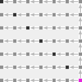
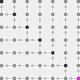
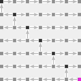
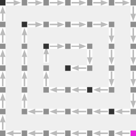
Figure 1: Four examples of many different orders the elements of the inverse $X$ may be computed when using Algorithm 1. The initial element is coloured purple.

In the remaining part of the paper we shall use and extend the following formulae, which corresponds to the lower left diagram in Figure 1:

$$\left.\begin{array}[]{l}\vspace*{-7.5ex}\\ \displaystyle q_{2}=\frac{-a_{2,1}}{a_{1,1}},\quad q_{k+1}=\frac{-a_{k+1,k}}{a_{k,k}+a_{k-1,k}q_{k}}\quad(1<k<n)\hskip 0.43057pt,\\ \displaystyle r_{n-1}=\frac{-a_{n,n-1}}{a_{n,n}},\quad r_{k-1}=\frac{-a_{k,k-1}}{a_{k,k}+a_{k,k+1}r_{k}}\quad(n>k>1)\hskip 0.43057pt,\\ \displaystyle x_{n,n}=\big{(}a_{n-1,n}q_{n}+a_{n,n}\big{)}^{-1}\hskip 0.43057pt,\\[7.5347pt] \displaystyle{\left.\begin{array}[]{l}x_{j,k-1}=q_{k}\hskip 0.86108ptx_{j,k}\quad(k\leq j\leq n)\\ x_{k-1,k-1}=r_{k-1}^{-1}x_{k,k-1}\end{array}\right\}}\quad(n\geq k>1)\hskip 0.43057pt,\\[10.76385pt] \displaystyle x_{j,k+1}=\big{(}a_{k+1,k}^{-1}a_{k,k+1}r_{k}\big{)}x_{j,k}\quad(1\leq j\leq k,\,\,\,1\leq k<n)\hskip 0.43057pt.\\[-4.30554pt] \end{array}\quad\right\}\vspace{0.75ex}$$ (3.7)

The above scheme is valid only if the inverse matrix $X$ has only non-zero elements in its lower triangle (note that this implies that $a_{k+1,k}\neq 0$ for $1\leq k<n$, and that each ratio that appears in (3.7) is finite — for proof, see Theorem 5 below). Now, we shall investigate the numerical properties of the algorithm based on (3.7).

Consider the elements $x_{s,k-1}$, $x_{s,k}$, $x_{s,k+1}$ ($k<s$) of $X$. They are computed as follows $x_{s,k}=q_{k+1}x_{s,k+1}$, $x_{s,k-1}=q_{k}\hskip 0.43057ptx_{s,k}$, which means that the numerically computed values satisfy $x_{s,k+1}^{-1}x_{s,k}=q_{k+1}(1+\gamma_{k+1})$ and $x_{s,k}^{-1}\hskip 0.43057ptx_{s,k-1}=q_{k}(1+\gamma_{k})$, where $|\gamma_{k}|,|\gamma_{k+1}|\leq\varepsilon$. From the first set of equations in (3.7), we readily obtain that for the numerically computed ratios $q_{k}$ and $q_{k+1}$ the following equality holds:

$$-a_{k+1,k}\hskip 0.43057ptq_{k+1}=a_{k,k}(1+\alpha_{k})+a_{k-1,k}\hskip 0.43057ptq_{k}(1+\beta_{k})\qquad(\hskip 0.43057pt|\alpha_{k}|\leq 2\varepsilon,\,\,\,|\beta_{k}|\leq 3\varepsilon)\hskip 0.43057pt$$

(again, we ignore the terms of order $\varepsilon^{2}$). By combining the two above results, we get

$$\big{|}a_{k+1,k}\hskip 0.43057ptx_{s,k+1}+a_{k,k}\hskip 0.43057ptx_{s,k}+a_{k-1,k}\hskip 0.43057ptx_{s,k-1}\big{|}\,\leq\,4\varepsilon\big{(}|a_{k,k}\hskip 0.43057ptx_{s,k}|+|a_{k-1,k}\hskip 0.43057ptx_{s,k-1}|\big{)}.$$ (3.8)

Every three adjacent elements in a column of the lower triangle of $X$ are computed exactly as follows:

$$x_{k-1,j}\, =\,x_{k,k}\hskip 0.43057ptq_{k}/r_{k-1}\hskip 0.43057ptq_{k-1}\hskip 0.43057ptq_{k-2}\cdots\hskip 0.43057ptq_{j+1}$$

$$x_{k,j}\, =\,x_{k+1,k}/r_{k}\hskip 0.43057ptq_{k}\hskip 0.43057ptq_{k-1}\cdots\hskip 0.43057ptq_{j+1},$$

$$x_{k+1,j}\, =\,x_{k+1,k}\hskip 0.43057ptq_{k}\hskip 0.43057ptq_{k-1}\cdots\hskip 0.43057ptq_{j+1}.\vspace{0.5ex}$$

Therefore, a bound analogous to (3.8) can be obtained with the leading factor $4$ replaced with some $c(j)$ that depends linearly on the column index $j$. Obviously, $c(j)\leq C(n)$ for some $C(n)=O(n)$. Similar $O(n)$-dependent bounds may be obtained (in a little more tedious way) for all remaining elements of the matrices $|XA-I|$ and $|AX-I|$ if we recall the relations (3.5).

In order to continue estimating the residual errors, we need the following, quite easy to prove lemma.

Lemma 3.

Let two matrices $F\in\mathbb{R}^{n\times n}$, $G\in\mathbb{R}^{n\times n}$ satisfy

$$|f_{ij}|\hskip 0.43057pt\leq\,|g_{ij}|+|g_{i,j+1}|\qquad(1\leq i\leq n,\,\,1\leq j\leq n)\hskip 0.43057pt,$$

where we assume that $g_{i,n+1}=0$ ($1\leq i\leq n$). Then,

$$\|F\hskip 0.86108pt\|_{1}\,\leq\,\hskip 0.43057pt2\hskip 0.43057pt\|G\hskip 0.43057pt\|_{1}\hskip 0.43057pt,\quad\|F\hskip 0.86108pt\|_{\infty}\,\leq\,\hskip 0.43057pt2\hskip 0.43057pt\|G\hskip 0.43057pt\|_{\infty}\hskip 0.43057pt,\quad\|F\hskip 0.86108pt\|_{F}\,\leq\,\hskip 0.43057pt2\hskip 0.43057pt\|G\hskip 0.43057pt\|_{F}\hskip 0.43057pt.$$ (3.9)

From the above lemma (or its several obvious generalisations), we immediately obtain that the inverse matrix $X$ computed numerically using the algorithm (3.7) satisfies (for simplicity, we restrict our attention to the $\|\cdot\|_{1}$ norm only)

$$\max\big{\{}\|XA-I\hskip 0.43057pt\|_{1},\,\|AX-I\hskip 0.43057pt\|_{1}\big{\}}\,\leq\,\varepsilon K(n)\|A\|_{1}\|X\|_{1},$$

where $K(n)=O(n)$. Note that a similar (even sharper) bound for $\|XA-I\|_{1}$ holds in the case of the unstable recursive algorithm based on (2.1). The important difference is the relation between $\|X\|_{1}$ and $\|A^{-1}\|_{1}$. We are convinced that if the inverse $X$ is computed using (3.7), then

$$\|X\|_{1}\,\leq\,\|A^{-1}\|_{1}\hskip 0.43057pt\big{(}1+\varepsilon J(n)\hskip 0.43057pt\mathrm{cond}(A)\big{)}$$ (3.10)

for some $J(n)=O(n)$. Possibly, the difference between $\|A^{-1}\|_{1}$ and $\|X\|_{1}$ may be larger than the right hand side of (3.10), but then $\|X\|_{1}<\|A^{-1}\|_{1}$. Our presumption is based on the fact that we are computing minimal solutions of the difference equations which correspond to the equations $AX=I=XA$ (the recurrences for ratios are carried out in the stable, towards-the-diagonal direction). In such a case, if we are moving away (along a row or a column) from the main diagonal, the elements of $X$ should not grow faster (or decrease slower) in modulus than the elements of $A^{-1}$, which, we think, implies the inequality (3.10). However, a formal proof of that assumption may be difficult.

Assuming that (3.10) holds, we obtain the following:

Conjecture 1.

If $A\in\mathbb{R}^{n\times n}$ is a non-singular matrix whose inverse has only non-zero elements in the lower triangle, and $\hskip 0.86108pt\varepsilon\hskip 0.43057ptn\hskip 0.86108pt\mathrm{cond}(A)<C$ for some constant $C$, then the inverse $X$ computed numerically by the algorithm (3.7) satisfies

$$\max\big{\{}\|XA-I\hskip 0.43057pt\|_{1},\hskip 0.86108pt\|AX-I\hskip 0.43057pt\|_{1}\big{\}}\hskip 0.86108pt\leq\,\varepsilon K(n)\hskip 0.43057pt\mathrm{cond}(A),$$ (3.11)

for some $K(n)=O(n)$.

Remark 1.

In the case of the algorithm of Lewis (c.f. [11] or Theorem 3), bounds similar to (3.8) can be derived for all non-diagonal elements of the residual matrices $AX-I$ and $XA-I$. For the diagonal elements, only $O(n)$-dependent bounds hold. This implies that the numerical properties of the algorithm (2.15)–(2.16) and the new algorithm based on (3.7) are comparable. Recall that if the Lewis algorithm is used together with (2.17), then moduli of some elements of the residual matrices may be almost as large as $\varepsilon\hskip 0.43057pt\mathrm{cond}(A)^{2}$.

Remark 2.

The important step in justifying Conjecture 1 is Lemma 3 which is not true in the case of the second matrix norm in general. The assertion of Lemma 3 is an immediate consequence of the fact that $\|G\|=\||G|\|_{\triangle}$ if $\triangle\in\{1,\infty,F\}$. In the case of the $\|\cdot\|_{2}$ norm, taking the moduli of all elements of a matrix may increase the norm by a factor proportional to $\sqrt{n}$ ($n$ is the matrix size). However, if $G=A$, where $A$ is a tridiagonal matrix, or $G=A^{-1}$, then $\|G\|\leq 2\||G|\|_{2}$, and the inequality similar to (3.9) is satisfied with the factor $2$ replaced by $4$. Consequently, we suspect the error estimation (3.11) to be also true in the case of the second matrix norm.

3.2 The extended ratio-based method

The last thing to do is to extend the scheme given in (3.7) so that it can be applied to an arbitrary non-singular tridiagonal matrix. Obviously, unlike, e.g., (2.17), the extension should preserve the very favourable numerical properties of the formulae (3.7), and also should not increase the computational complexity. To achieve the goal, several conditions need to be fulfilled. The computations may include only one initial element, all other elements of the inverse matrix $X$ should be computed from another element (adjacent if possible) by only one multiplication (or division), $x_{ij}=c_{ij}x_{i-q,j-r}$, in such a way that each relation between two elements is a direct consequence of the equations $AX=I=XA$. Of course, the number of additional arithmetic operations should depend linearly on the matrix size $n$.

In order to do so, we need a complete characterisation of possible shapes of blocks of zeros in the inverse matrix $X$.

Theorem 5.

Let $A\in\mathbb{R}^{n\times n}$ be a non-singular tridiagonal matrix, and $X=A^{-1}$.
a) If $\hskip 0.43057pta_{k+1,k}=0$, then $x_{ij}=0$ for all $\hskip 0.43057ptk+1\leq i\leq n$ and $1\leq j\leq k$ ($1\leq k\leq n-1$).
b) If $\hskip 0.43057pta_{k-1,k}=0$, then $x_{ij}=0$ for all $\hskip 0.43057pt1\leq i\leq k-1$ and $k\leq j\leq n$ ($2\leq k\leq n$).
c) If $\hskip 0.43057pt|q_{k}|=\infty$ or, equivalently, $|\hat{r}_{k}|=\infty$, then $\hskip 0.43057ptx_{s,k}=0$ for $\hskip 0.43057ptk\leq s\leq n$, and $\hskip 0.43057ptx_{k,j}=0$ for $\hskip 0.43057ptk\leq j\leq n$ ($2\leq k\leq n$).
d) If $\hskip 0.43057pt|r_{k}|=\infty$ or, equivalently, $|\hat{q}_{k}|=\infty$, then $\hskip 0.43057ptx_{k,j}=0$ for $\hskip 0.43057pt1\leq j\leq k$, and $\hskip 0.43057ptx_{s,k}=0$ for $\hskip 0.43057pt1\leq s\leq k$ ($1\leq k\leq n-1$).
e) Each block of zeros in the inverse matrix $X$ may consist only of the four different types of blocks described above.

Proof.

The above assertions are a direct consequence of Theorem 4 and (2.17). ∎

Before we proceed, one more problem, related to the computation of ratios, has to be solved. Observe that if $a_{k,k-1}=0$, then $q_{k}=0$. In this case, the relation (3.5) remains true, but it cannot be used to compute the ratio $\hat{r}_{k}=a_{k,k-1}^{-1}a_{k-1,k}\hskip 0.43057ptq_{k}$. The following lemma delivers a scheme that allows to compute all the ratios in every case, without sacrificing the relation (3.5).

Lemma 4.

a) The ratios $q_{k}=x_{j,k}^{-1}\hskip 0.43057ptx_{j,k-1}$ and $\hat{r}_{k}=x_{k,j}^{-1}\hskip 0.43057ptx_{k-1,j}$ ($1<k\leq n$, $j\geq k$) satisfy

$$\left.\begin{array}[]{l}\vspace{-4.5ex}\\ q_{2}=-a_{1,1}^{-1}\hskip 0.43057pta_{2,1}\hskip 0.43057pt,\qquad q_{k+1}=-s_{k}^{-1}\hskip 0.43057pta_{k+1,k}\hskip 0.43057pt,\\ \hat{r}_{2}=-a_{1,1}^{-1}\hskip 0.43057pta_{1,2}\hskip 0.43057pt,\qquad\hat{r}_{k+1}=-s_{k}^{-1}\hskip 0.43057pta_{k,k+1}\hskip 0.43057pt,\end{array}\quad\right\}\quad(1<k<n)\vspace{-1ex}$$ (3.12)

where

$$s_{k}=a_{k,k}+a_{k-1,k}\hskip 0.43057ptq_{k}\qquad(1<k<n)\hskip 0.43057pt.\vspace{1.5ex}$$ (3.13)

b) The ratios $\hat{q}_{k}=x_{j,k}^{-1}\hskip 0.43057ptx_{j,k+1}$ and $r_{k}=x_{k,j}^{-1}\hskip 0.43057ptx_{k+1,j}$ ($1\leq k<n,\,\,j\leq k$) satisfy

$$\left.\begin{array}[]{l}\vspace{-4.5ex}\\ \hat{q}_{n-1}=-a_{n,n}^{-1}\hskip 0.43057pta_{n-1,n}\hskip 0.43057pt,\qquad\hat{q}_{k-1}=-t_{k}^{-1}\hskip 0.43057pta_{k-1,k}\hskip 0.43057pt,\\ r_{n-1}=-a_{n,n}^{-1}\hskip 0.43057pta_{n,n-1}\hskip 0.43057pt,\qquad r_{k-1}=-t_{k}^{-1}\hskip 0.43057pta_{k,k-1}\hskip 0.43057pt,\end{array}\quad\right\}\quad(n>k>1)\vspace{-1ex}$$ (3.14)

where

$$t_{k}=a_{k,k}+a_{k,k+1}\hskip 0.43057ptr_{k}\qquad(2\leq k<n)\hskip 0.43057pt.\vspace{1ex}$$ (3.15)

Proof.

The formulae (3.12) and (3.14) follow immediately from the definition of the ratios and the relation (3.5) if we additionally assume the standard convention that $c/0=\infty$ for $c>0$, $c/0=-\infty$ for $c<0$, and $c/\infty=0$ for $|c|<\infty$. ∎

Remark 3.

Note that the values $s_{k}$ and $t_{k}$ do not have to be remembered, i.e. in practical implementation, can be replaced by a single variable.

Remark 4.

By (3.5), the last terms in (3.13) and (3.15) can be replaced with $a_{k,k-1}\hskip 0.43057pt\hat{r}_{k}$ and $a_{k+1,k}\hskip 0.43057pt\hat{q}_{k}$, respectively. The method proposed in this paper has slightly better numerical properties if the ”leading” ratios — the ones that appear in (3.13) and (3.15) — belong to the same triangle, i.e. if the leading pairs are: $\{q_{k}\}$ and $\{r_{k}\}$, or : $\{\hat{q}_{k}\}$ and $\{\hat{r}_{k}\}$.

Now, we may formulate the main result of this Section.

Theorem 6.

Let $A\in\mathbb{R}^{n\times n}$ be a non-singular tridiagonal matrix, and $X=A^{-1}$. Let us assume that the ratios $q_{k}$, $\hat{r}_{k}$ ($2\leq k\leq n$), and $\hat{q}_{k}$, $r_{k}$ ($1\leq k\leq n-1$) are given by (3.12) and (3.14).
a) For $2\leq k\leq n$, if $|q_{k}|<\infty$, then

$$x_{s,k-1}=q_{k}\hskip 0.43057ptx_{s,k}\quad(k\leq s\leq n)\hskip 0.43057pt,\vspace{-0.5ex}$$ (3.16)

otherwise, for  $k<s\leq n$, we have

$$x_{s,k-1}\hskip 0.86108pt=\left\{\begin{array}[]{ll}\vspace*{-4.125ex}\\ a_{n-1,n}^{-1}&\,\mathrm{if}\quad k=n\hskip 0.43057pt,\\ -a_{k+1,k}a_{k-1,k}^{-1}\hskip 0.43057ptx_{s,k+1}&\,\mathrm{if}\quad k<n\hskip 0.43057pt.\end{array}\right.$$ (3.17)

In addition, if $|q_{k}|=\infty$, then for $2\leq k<n$,

$$x_{k,k-1}\hskip 0.86108pt=\left\{\begin{array}[]{ll}\vspace*{-4.33ex}\\ r_{k}^{-1}x_{k+1,k-1}&\,\mathrm{if}\quad r_{k}\neq 0\hskip 0.43057pt,\\ -a_{k+1,k+2}a_{k+1,k}^{-1}\hskip 0.43057ptx_{k+2,k-1}&\,\mathrm{if}\quad r_{k}=0,\,a_{k+1,k}\neq 0\hskip 0.43057pt,\\ -a_{k,k+1}a_{k-1,k}^{-1}\hskip 0.43057pt\hat{q}_{k}^{\hskip 0.60275pt-1}x_{k+1,k+1}&\,\mathrm{if}\quad r_{k}=0,\,a_{k+1,k}=0,\,\hat{q}_{k}\neq 0\hskip 0.43057pt,\\ a_{k+1,k+2}a_{k-1,k}^{-1}\hskip 0.43057ptx_{k+2,k+1}&\,\mathrm{if}\quad r_{k}=0,\,a_{k+1,k}=0,\,\hat{q}_{k}=0,\,a_{k,k+1}\neq 0\hskip 0.43057pt,\\ a_{k-1,k}^{-1}&\,\,\mathrm{otherwise}\hskip 0.43057pt.\end{array}\right.$$ (3.18)

b) For $2\leq k\leq n$, the diagonal element $\hskip 0.43057ptx_{k-1,k-1}$ satisfies

$$x_{k-1,k-1}\hskip 0.86108pt=\left\{\begin{array}[]{ll}\vspace*{-4.33ex}\\ r_{k-1}^{-1}x_{k,k-1}&\,\mathrm{if}\quad r_{k-1}\neq 0\hskip 0.43057pt,\\ \hat{r}_{k}\hskip 0.43057pt\hat{q}_{k-1}^{\hskip 0.60275pt-1}x_{k,k}&\,\mathrm{if}\quad r_{k-1}=0,\,\hat{q}_{k-1}\neq 0\hskip 0.43057pt,\\ -a_{k,k+1}a_{k,k-1}^{-1}x_{k+1,k-1}&\,\mathrm{if}\quad r_{k-1}=0,\,\hat{q}_{k-1}=0,\,a_{k,k-1}\neq 0\hskip 0.43057pt,\\ -a_{k,k+1}a_{k-1,k}^{-1}\hskip 0.43057pt\hat{r}_{k}\hskip 0.43057ptx_{k+1,k}&\,\mathrm{if}\quad r_{k-1}=0,\,\hat{q}_{k-1}=0,\,a_{k,k-1}=0,\,a_{k-1,k}\neq 0\hskip 0.43057pt,\\ \big{(}a_{k-2,k-1}q_{k-1}+a_{k-1,k-1}\big{)}^{-1}&\,\mathrm{otherwise}\hskip 0.43057pt.\end{array}\right.$$ (3.19)

c) For $1\leq k\leq n-1$, if $|\hat{q}_{k}|<\infty$, then

$$x_{s,k+1}=\hat{q}_{k}\hskip 0.43057ptx_{s,k}\quad(1\leq s\leq k)\hskip 0.43057pt,\vspace{-0.5ex}$$ (3.20)

otherwise, for  $1\leq s<k$ we have

$$x_{s,k+1}\hskip 0.86108pt=\left\{\begin{array}[]{ll}\vspace*{-4.125ex}\\ a_{1,2}a_{2,1}^{-1}x_{2,1}&\,\mathrm{if}\quad k=1\hskip 0.43057pt,\\ -a_{k-1,k}a_{k+1,k}^{-1}\hskip 0.43057ptx_{s,k-1}&\,\mathrm{if}\quad k>1\hskip 0.43057pt.\end{array}\right.$$ (3.21)

In addition, if $|\hat{q}_{k}|=\infty$, then for $1<k\leq n-1$

$$x_{k,k+1}\hskip 0.86108pt=\left\{\begin{array}[]{ll}\vspace*{-4.33ex}\\ \hat{r}_{k}^{\hskip 0.60275pt-1}x_{k-1,k+1}&\,\mathrm{if}\quad\hat{r}_{k}\neq 0\hskip 0.43057pt,\\ -a_{k-1,k-2}a_{k-1,k}^{-1}\hskip 0.43057ptx_{k-2,k+1}&\,\mathrm{if}\quad\hat{r}_{k}=0,\,a_{k-1,k}\neq 0\hskip 0.43057pt,\\ -a_{k,k-1}a_{k+1,k}^{-1}\hskip 0.43057ptq_{k}^{-1}\hskip 0.43057ptx_{k-1,k-1}&\,\mathrm{if}\quad\hat{r}_{k}=0,\,a_{k-1,k}=0,\,q_{k}\neq 0\hskip 0.43057pt,\\ a_{k-1,k-2}a_{k+1,k}^{-1}\hskip 0.43057ptx_{k-2,k-1}&\,\mathrm{if}\quad\hat{r}_{k}=0,\,a_{k-1,k}=0,\,q_{k}=0,\,a_{k,k-1}\neq 0\hskip 0.43057pt,\\ a_{k,k+1}a_{k+1,k}^{-1}\hskip 0.43057ptx_{k+1,k}&\,\mathrm{otherwise}\hskip 0.43057pt.\end{array}\right.\vspace{-0.5ex}$$ (3.22)

Proof.

The formulae (3.16)–(3.22) result from the equations $AX=I=XA$, the relations (2.13) and (3.5), and from Theorem 5. The complete proof is not very difficult, but is quite long. Therefore, we shall justify only the one before last formula in (3.18), which — we think — is the most difficult one to prove.

From Theorem 5, we conclude that if $|q_{k}|=\infty$ and $\hat{q}_{k}=a_{k+1,k}=0$, then $x_{k+1,k+1}=0$ and $x_{ij}=0$ for $k+1\leq i\leq n$, $1\leq j\leq n$. This implies that the closest non-zero element to $x_{k,k-1}$ in the lower triangle is $x_{k+2,k+1}$, but there is no ”multiplicative path” between these two elements that would lead through the lower triangle only. However, in this case, we also (by Theorem 5) know that $x_{k,k+2}=0$, $x_{k-1,k+1}=0$, and that $x_{k+1,k+2}\neq 0$, $x_{k-1,k+2}\neq 0$, and $x_{k-1,k}\neq 0$, as $A$ is non-singular and $a_{k,k+1}\neq 0$. Consequently, from the equations $AX=I$ and $XA=I$, and from (2.13), we have

$$\begin{array}[]{r@{\,\,=\,\,}l}\displaystyle x_{k,k-1}&\displaystyle\frac{a_{k,k-1}}{a_{k-1,k}}\hskip 0.86108ptx_{k-1,k}=\frac{a_{k,k-1}}{a_{k-1,k}}\hskip 0.86108pt\left(-\frac{a_{k+2,k+1}}{a_{k,k+1}}\hskip 0.86108ptx_{k-1,k+2}\right)\\ &\displaystyle-\frac{a_{k,k-1}}{a_{k-1,k}}\hskip 0.86108pt\frac{a_{k+2,k+1}}{a_{k,k+1}}\hskip 0.86108pt\left(-\frac{a_{k,k+1}}{a_{k,k-1}}\hskip 0.86108ptx_{k+1,k+2}\right)=\frac{a_{k+2,k+1}}{a_{k-1,k}}\hskip 0.86108pt\left(\frac{a_{k+1,k+2}}{a_{k+2,k+1}}\hskip 0.86108ptx_{k+2,k+1}\right)\\ &\displaystyle\frac{a_{k+2,k+1}}{a_{k-1,k}}\hskip 0.86108ptx_{k+2,k+1}\hskip 0.43057pt.\end{array}\vspace{0.25ex}$$

All other equations of Theorem 6 can be proved in an analogous way. What still may need a little more explanation is that, e.g., the second and fourth equations of (3.18) refer to the element $a_{k+1,k+2}$ which does not exist if $k=n-1$. However, it can be proved (using. e.g., Theorem 5) that if $A$ is a non-singular matrix, then the conditions required by these two equations can be satisfied only for $k<n-1$. ∎

The formulae (3.16)–(3.22) may be considered as a detailed description of the new algorithm which can invert any non-singular tridiagonal matrix $A$ if we add one initial step: $\hskip 0.43057ptx_{n,n}=(a_{n-1,n}q_{n}+a_{n,n})^{-1}$. The algorithm is not as elegant as, e.g, pivoting in the case of Gaussian elimination, but has a very important feature: has the same complexity as its basic version, i.e. $n^{2}+O(n)$. What is even more important, the new extended algorithm has the same numerical properties as the one given by (3.7). Some doubts may be related to the last formulae of (3.18) and (3.19), where we, in fact, use another starting element. However, these two cases correspond to the situation, where $A$ is a block diagonal matrix, and so

$$A^{-1}\,=\,\,\begin{pmatrix}F&0\,\\ 0&G\,\end{pmatrix}^{-1}=\,\,\,\begin{pmatrix}F^{-1}&0\\ 0&G^{-1}\end{pmatrix}.$$ (3.23)

In this particular case only, the matrices $F$ and $G$ can be inverted independently, as they are in no way related in the equations $AX=I=XA$. Note that with the proposed scheme, there is no need for special treatment of cases analogous to (3.23), as the initial element for the inverse matrix $F^{-1}$ is computed — as one could say — on the way.

The only limitation of the proposed new method for inverting general tridiagonal matrices $A\in\mathbb{R}^{n\times n}$ is that it requires $n\geq 2$. Obviously, if $n=1$, then $X=[a_{1,1}^{-1}\hskip 0.43057pt]$.

References

- [1] E. Asplund, Inverse of matrices which satisfy for , Math. Scand. 7 (1959), 57–60.
- [2] P. Concus, G. H. Golub, G. Meurant, Block preconditioning for the conjugate gradient method, SIAM J. Sci. and Stat. Comput. 6(1) (1985), 220–252.
- [3] B. N. Datta, Numerical Linear Algebra and Applications, second ed., SIAM, Philadelphia, 2010.
- [4] J. J. Du Croz, N. J. Higham, Stability of methods for matrix inversion, IMA J. Numer. Anal. 12 (1992), 1–19.
- [5] J. Jain; H. Li, S. Cauley, C. Koh, V. Balakrishnan, Numerically Stable Algorithms for Inversion of Block Tridiagonal and Banded Matrices, ECE Technical Reports, paper 357 (2007).
- [6] M. El-Mikkawy, E.-D. Rahmo, A new recursive algorithm for inverting general tridiagonal and anti-tridiagonal matrices, Appl. Math. Comput. 204 (2008), 368–372.
- [7] D. K. Faddeev, Properties of the inverse of a Hessenberg matrix, Numerical Methods and Computational Issues 5 (1981), V. P. Ilin and V. N. Kublanovskaya, eds. (in Russian).
- [8] W. Gautschi, Computational aspects of three-term recurrence relations, SIAM Rev. 9 (1967), 24–82.
- [9] A. D. A. Hadj, M. Elouafi, A fast numerical algorithm for the inverse of a tridiagonal and pentadiagonal matrix, Appl. Math. Comput. 202 (2008), 441–445.
- [10] N. J. Higham, Accuracy and Stability of Numerical Algorithms, second ed., SIAM, Philadelphia, 2002.
- [11] J. W. Lewis, Inversion of tridiagonal matrices, Numer. Math. 38 (1982), 333–345.
- [12] J. C. P. Miller, Bessel Functions. Part II, Math. Tables, vol. 10, British Assoc. Adv. Sci., Cambridge Univ. Press, 1952.
- [13] J. Wimp, Computation with recurrence relations, Applicable Mathematics Series, Pitman, London, 1984.