Higher-order in time “quasi-unconditionally stable” ADI solvers for the compressible Navier-Stokes equations
in 2D and 3D curvilinear domains

Abstract

This paper introduces alternating-direction implicit (ADI) solvers of higher order of time-accuracy (orders two to six) for the compressible Navier-Stokes equations in two- and three-dimensional curvilinear domains. The higher-order accuracy in time results from 1) An application of the backward differentiation formulae time-stepping algorithm (BDF) in conjunction with 2) A BDF-like extrapolation technique for certain components of the nonlinear terms (which makes use of nonlinear solves unnecessary), as well as 3) A novel application of the Douglas-Gunn splitting (which greatly facilitates handling of boundary conditions while preserving higher-order accuracy in time). As suggested by our theoretical analysis of the algorithms for a variety of special cases, an extensive set of numerical experiments clearly indicate that all of the BDF-based ADI algorithms proposed in this paper are “quasi-unconditionally stable” in the following sense: each algorithm is stable for all couples $(h,\Delta t)$ of spatial and temporal mesh sizes in a problem-dependent rectangular neighborhood of the form $(0,M_{h})\times(0,M_{t})$. In other words, for each fixed value of $\Delta t$ below a certain threshold, the Navier-Stokes solvers presented in this paper are stable for arbitrarily small spatial mesh-sizes. The second order formulation has further been rigorously shown to be unconditionally stable for linear hyperbolic and parabolic equations in two-dimensional space. Although implicit ADI solvers for the Navier-Stokes equations with nominal second-order of temporal accuracy have been proposed in the past, the algorithms presented in this paper are the first ADI-based Navier-Stokes solvers for which second order or better accuracy has been verified in practice under non-trivial (non-periodic) boundary conditions.

1 Introduction

The direct numerical simulation of fluid flow at high Reynolds numbers presents a number of significant challenges [19]—including the presence of structures such as boundary layers, eddies, vortices and turbulence, whose accurate spatial discretization requires use of fine spatial meshes. Simulation of such flows by means of explicit solvers is difficult, even on massively parallel super computers, in view of the severe restrictions on time-steps required for stability: the time-step must scale like the square of the spatial mesh-size. Classical implicit solvers do not suffer from such time-step restrictions but they do require solution of large systems of equations at each time step, and they can therefore be extremely expensive as well. The celebrated Beam and Warming method [4, 3] provides one of the most attractive alternatives to explicit and classical implicit algorithms. Based on the the Alternating Direction Implicit method [35] (ADI), the Beam and Warming scheme enables stable solution of the compressible Navier-Stokes equations without recourse to either nonlinear iterative solvers or solution of large linear systems at each time-step.

Significant efforts [41, 18, 37, 21, 40, 27] have centered around the ideas first put forth in the celebrated papers [4, 3], focusing, in particular, on enhancing stability and restoring the (nominal) second-order of accuracy inherent in the original derivation of the method. (The discussion in Section 3.5 suggests that, indeed, the overall accuracy of a time-marching ADI scheme based on second-order time-stepping may drop to first-order of accuracy in time if boundary conditions at intermediate-times are not enforced with the correct accuracy order; see also [6, 31].) The aforementioned modifications of the algorithms [4, 3] incorporate various kinds of Newton-like subiterations to reduce the errors arising from the approximation of the nonlinear terms while maintaining stability. Unfortunately, however, no numerical examples have been provided that demonstrate second-order time-accuracy for the modified algorithms—even though in all such cases nominally second-order time-stepping schemes are used. Still, as demonstrated by the numerical results presented in this paper (see e.g. Figures 3, 4 and 5 and associated discussion), high-order time accuracy may be highly advantageous in the treatment of long-time simulations or highly-inhomogeneous flows—for which the temporal dispersion inherent in low-order approaches would make it necessary to use inordinately small time-steps.

The present paper (Part I in a two-part contribution) introduces ADI solvers of higher orders of time-accuracy (orders $s=2$ to 6) for the compressible Navier-Stokes equations in two- and three-dimensional curvilinear domains; for definiteness spectral Chebyshev and Fourier collocation spatial discretizations are used throughout this paper. The new ADI algorithms successfully address the difficulties discussed above: (i) They (provably) enjoy high orders of time-accuracy (orders two to six) even in presence of general (and, in particular, non-periodic) boundary conditions; (ii) They do not require use of iterative nonlinear solvers for accuracy or stability, and they rely, instead, on a BDF-like extrapolation technique [9] for certain components of the nonlinear terms; and, as established in Part II [8], (iii) They possess favorable stability properties, with rigorous unconditional-stability proofs for constant coefficient hyperbolic and parabolic equations for $s=2$, and demonstrating in practice quasi-unconditional stability for $2\leq s\leq 6$ (Definition 1 in Section 4.2).

The ADI split and extrapolation techniques mentioned above give rise to certain two-point boundary-values problems for second-order systems of ODEs with variable coefficients. The specific methodologies utilized to solve such ODE systems depends significantly on the method used for spatial approximation. If a finite-difference approximation is used, then the solution of the ODE systems under consideration entails inversion of a linear system with a banded system matrix, which can be treated efficiently by means of sparse LU decompositions [20]. If spectral methods are used, as in this paper, in turn, then the ODE solution requires inversion of a full non-sparse linear system. In order to tackle such problems efficiently we resort to use of the GMRES algorithm [38] in conjunction with a finite-difference preconditioner, as detailed in Section 5.1. The resulting overall Navier-Stokes solvers are applicable to curvilinear coordinate systems in general domains; an accuracy-order-preserving spectral filter is used in our scheme to ensure stability.

Although quite fast when compared to other implicit algorithms, the implicit solvers introduced in this paper are more expensive per time-step than a similarly discretized explicit solver. Nevertheless, implicit solvers of high-order time accuracy such as the ones introduced in what follows may play crucial roles in the treatment of long-time simulations, highly-inhomogeneous flows, complex physical boundaries as well as steep boundary layers. For such problems the requirements of fine spatial discretization meshes—which may be needed for flow and/or geometry resolution—could necessitate use of very small time-steps, in view of the restrictive CFL constraints inherent in explicit solvers for Navier-Stokes problems, and thus, possibly, to inordinately large computing times. Extensions of these algorithms to the multi-domain overlapping-patch context [7] as well as other types of spatial discretizations, including finite-differences [30] and Fourier Continuation [10, 1], are currently in progress and will be presented elsewhere. In particular, the present curvilinear domain algorithms are ideally suited as single-domain implicit components of general multi-domain implicit/explicit solvers [13].

This paper is organized as follows: after notations are introduced in Section 2, Section 3 presents the proposed BDF-ADI methodology in full detail. Section 4 discusses the stability properties of the proposed methods, with reference to the stability proofs and numerical demonstrations put forth in Part II. Section 5 then presents details of our algorithmic implementations, and Section 6 demonstrates the stability and accuracy of the proposed algorithms by means of a variety of numerical results. Concluding remarks, finally, are presented in Section 7.

2 Preliminaries

We consider the compressible Navier-Stokes equations for the velocity $\mathbf{u}$, temperature $T$ and density $\rho$ in a perfect gas in a $d$-dimensional domain $\Omega\subset\mathbb{R}^{d}$ ($d=2$ or $d=3$). For definiteness we assume the pressure $p$, density $\rho$, temperature $T$ are related by the ideal gas law $p=\rho RT$ with gas constant $R$. The heat flux $q$ and the temperature gradient $\nabla T$, in turn, are assumed to satisfy the isotropic Fourier law $q=-\kappa\,\nabla T$ for a certain (temperature-dependent) thermal conductivity constant $\kappa$. Using characteristic values $L_{0}$, $u_{0}$, $\rho_{0}$, $T_{0}$, $\mu_{0}$ and $\kappa_{0}$ for length, velocity, density, temperature, viscosity and heat conductivity, respectively, the Navier-Stokes equations under consideration can be expressed in the non-dimensional form [42]

$$\rho_{t}+\nabla\cdot(\rho\mathbf{u}) = 0$$ (1a)

$$\mathbf{u}_{t}+\mathbf{u}\cdot\nabla\mathbf{u}+\frac{1}{\gamma\mathrm{Ma}^{2}}\frac{1}{\rho}\nabla(\rho T) = \frac{1}{\mathrm{Re}}\frac{1}{\rho}\nabla\cdot\boldsymbol{\sigma}$$ (1b)

$$T_{t}+\mathbf{u}\cdot\nabla T+(\gamma-1)T\nabla\cdot\mathbf{u} = \frac{\gamma}{\mathrm{Re}\mathrm{Pr}}\frac{1}{\rho}\nabla\cdot(\kappa\nabla T)+\frac{\gamma(\gamma-1)\mathrm{Ma}^{2}}{\mathrm{Re}}\frac{1}{\rho}\Phi$$ (1c)

($\mathbf{u}=(u_{i})$, $\boldsymbol{\sigma}=(\sigma_{ij})$, $i,j=1,\dots,d$) where $\gamma=c_{p}/c_{v}$ is the ratio of specific heats, $\mathrm{Re}=\rho_{0}u_{0}L_{0}/\mu_{0}$ is the Reynolds number and $\mathrm{Ma}=u_{0}/\sqrt{\gamma RT_{0}}$ is the Mach number (with gas constant $R=c_{p}-c_{v}$), and where $\mathrm{Pr}=\mu_{0}c_{p}/\kappa_{0}$ is the Prandtl number. The non-dimensional primitive variables in these equations are the velocity vector $\mathbf{u}$, the density $\rho$ and the temperature $T$; the quantities $\boldsymbol{\sigma}$ and $\Phi$, in turn, denote the Newtonian deviatoric stress tensor and the viscous dissipation function, respectively: letting $I$ denote the identity tensor, we have

$$\boldsymbol{\sigma}=\mu\left(\nabla\mathbf{u}+\nabla\mathbf{u}^{\mathrm{T}}-\frac{2}{3}(\nabla\cdot\mathbf{u})\mathbf{I}\right)\quad\mbox{and}\quad\Phi=\sum_{ij}\sigma_{ij}\partial_{x_{i}}u_{j}.$$

For definiteness we assume $\mu$ and $\kappa$ are functions of temperature alone—as they are, for example, under Sutherland’s law [42, pp. 28–30]

$$\kappa=\frac{1+S_{\kappa}}{T+S_{\kappa}}T^{3/2}\quad\mbox{and}\quad\mu=\frac{1+S_{\mu}}{T+S_{\mu}}T^{3/2},$$ (2)

where $S_{\kappa}$ and $S_{\mu}$ are the non-dimensionalized Sutherland constants.

Letting $Q=(\mathbf{u}^{\mathrm{T}},T,\rho)^{\mathrm{T}}$ denote the full $(d+2)$-dimensional solution vector, the equations (1) can be expressed in the form

$$Q_{t}=\mathcal{P}(Q,t)\quad,\quad x\in\Omega\quad,\quad t\geq 0$$ (3)

where $\mathcal{P}$ is a vector-valued nonlinear differential operator. Note the $t$ dependence in the operator $\mathcal{P}$ which allows for the presence of time-dependent source terms. The system is completed by means of the relevant boundary conditions for a given configuration; see e.g. [42, Sec. 1-4].

Remark 1.

For notational simplicity our description of the BDF-ADI algorithms assumes that no-slip boundary conditions of the form

$$\left.\begin{pmatrix}\mathbf{u}\\ T\end{pmatrix}\right|_{\partial D}=\begin{pmatrix}g^{\mathbf{u}}\\ g^{T}\end{pmatrix}$$ (4)

are prescribed, where $g^{\mathbf{u}}$ and $g^{T}$ are given functions defined on $\partial D$. Certainly, other relevant types of boundary conditions can be incorporated within the proposed framework—Section 6 includes an example of unsteady boundary layer flow that incorporates no-slip boundary conditions at a rough boundary as well as inflow and absorbing boundary conditions.

3 BDF-ADI methodology

This section introduces the proposed BDF-ADI approach. Throughout this section derivations and formulae are given for problems in $d=3$ spatial dimensions but, in all cases, the treatment can be applied easily to obtain the corresponding two-dimensional counterparts. The numerical examples in Section 6, in particular, include applications to problems in both two- and three-dimensional space.

3.1 Quasilinear-like Cartesian formulation

The derivation of the proposed BDF-ADI method relies on a certain quasilinear-like formulation of the Navier-Stokes equations. To motivate the introduction of this concept we note that provided $\mu$ and $\kappa$ are constant and the viscous dissipation function $\Phi$ is neglected, the Navier-Stokes equations under consideration may be expressed in the quasilinear form

$$Q_{t} +M^{x,1}(Q)\frac{\partial}{\partial x}Q+M^{y,1}(Q)\frac{\partial}{\partial y}+M^{z,1}(Q)\frac{\partial}{\partial z}Q$$

$$+M^{x,2}(Q)\frac{\partial^{2}}{\partial x^{2}}Q+M^{y,2}(Q)\frac{\partial^{2}}{\partial y^{2}}Q+M^{z,2}(Q)\frac{\partial^{2}}{\partial z^{2}}Q$$

$$+M^{xy}(Q)\frac{\partial^{2}}{\partial x\partial y}Q+M^{xz}(Q)\frac{\partial^{2}}{\partial x\partial z}Q+M^{yz}(Q)\frac{\partial^{2}}{\partial y\partial z}Q+M^{0}(Q)Q$$

$$=0,$$ (5)

where the various $M$ matrices ($M^{x,1}$, $M^{x,2}$ etc.) are matrix-valued functions of $Q$. Such a formulation can be made to stand even if $\Phi$ is not neglected and/or $\mu$ and $\kappa$ are non-constant, provided the $M$ matrices are allowed to incorporate certain derivative terms. For example, terms such as $u_{x}^{2}$ which arise in the dissipation function $\Phi$ can be incorporated in such a formulation by including one $u_{x}$ term in the matrix $M^{x,1}$ and the second $u_{x}$ term in the vector $\partial_{x}Q$. Similarly, expanding the product $\mu(T)_{x}u_{y}$ (that arises in in the term $\nabla\cdot\boldsymbol{\sigma}$) by means of the chain rule,

$$\mu(T)_{x}u_{y} =\mu^{\prime}(T)T_{x}u_{y}$$

$$=\left(\frac{1}{2}\mu^{\prime}(T)T_{x}\right)u_{y}+\left(\frac{1}{2}\mu^{\prime}(T)u_{y}\right)T_{x},$$ (6)

the two quantities in parentheses can be included in the matrices $M^{y,1}$ and $M^{x,1}$ respectively. (We note that while the expression (3.1) treats the factors in the product $T_{x}u_{y}$ in an symmetric manner, other alternatives may be useful as well.) The $M$ matrices resulting from this approach are presented in Appendix A.

Upon temporal discretization the proposed algorithms treat implicitly all spatial derivatives in equations (3.1) not included in the $M$ matrices, and they approximate the corresponding $M$ coefficients by means of certain explicit time extrapolations. Full algorithmic details in these regards, allowing for possible use of curvilinear coordinates, are presented in sections 3.2 through 3.5.

3.2 Quasilinear-like curvilinear formulation

Let $x=x(\xi,\eta,\zeta)$, $y=y(\xi,\eta,\zeta)$, $z=z(\xi,\eta,\zeta)$ define a smooth invertible mapping from the the $(\xi,\eta,\zeta)$ computational domain (which we take to be the cube $D=[\ell_{1},\ell_{2}]^{3}$ for some real numbers $\ell_{1}$ and $\ell_{2}$) to the physical domain $\Omega\subset\mathbb{R}^{3}$. With minor notational abuses, we will denote the corresponding inverse mapping by $\xi=\xi(x,y,z)$, $\eta=\eta(x,y,z)$, $\zeta=\zeta(x,y,z)$, and we will write $Q(\xi,\eta,\zeta)=Q(x(\xi,\eta,\zeta),y(\xi,\eta,\zeta),z(\xi,\eta,\zeta))$. A formulation in terms of the variables $(\xi,\eta,\zeta)$ is obtained by invoking the chain rule: the derivatives with respect to $x$, $y$, and $z$ in equation (3.1) are expressed in terms of derivatives with respect to $\xi$, $\eta$, and $\zeta$ of the unknown $Q$ and certain “metric terms” given by derivatives of $\xi$, $\eta$, and $\zeta$ with respect to the Cartesian variables. Using these variables in (3.1) and collecting terms we obtain an equation for $Q=Q(\xi,\eta,\zeta,t)$:

$$Q_{t} +M^{\xi,1}(Q)\frac{\partial}{\partial\xi}Q+M^{\eta,1}(Q)\frac{\partial}{\partial\eta}+M^{\zeta,1}(Q)\frac{\partial}{\partial\zeta}Q$$

$$+M^{\xi,2}(Q)\frac{\partial^{2}}{\partial\xi^{2}}Q+M^{\eta,2}(Q)\frac{\partial^{2}}{\partial\eta^{2}}Q+M^{\zeta,2}(Q)\frac{\partial^{2}}{\partial\zeta^{2}}Q$$

$$+M^{\xi\eta}(Q)\frac{\partial^{2}}{\partial\xi\partial\eta}Q+M^{\xi\zeta}(Q)\frac{\partial^{2}}{\partial\xi\partial\zeta}Q+M^{\eta\zeta}(Q)\frac{\partial^{2}}{\partial\eta\partial\zeta}Q+M^{0}(Q)Q$$

$$=0$$ (7)

for $(\xi,\eta,\zeta)\in D$, where the matrices $M^{\xi,1}(Q)$ (which, per the discussion in Section 3.1, generally contain derivatives of $Q$ with regards to $(\xi,\eta,\zeta)$) can be obtained by incorporating the various metric terms in the corresponding Cartesian matrices; see e.g. [24]. Explicit expressions for the $M$ matrices in equation (3.2) are presented in Appendix A.

3.3 BDF temporal semi-discretization and treatment of non-linearities.

To produce our BDF-based numerical solver for the system (1) we first lay down a semi-discrete approximation of this equation—discrete in time but continuous in space—on the basis of the BDF multistep method of order $s$ [29, Ch. 3.12]. Considering the concise expression (3) we let $Q^{j}$ denote the numerical approximation of $Q$ at time $t=t^{j}$ and we approximate $Q_{t}$ at $t=t^{n+1}$ by the time derivative of the $(d+2)$-dimensional vector $V=V(t)$ of polynomials of degree $s$ in the variable $t$ that interpolates the vector values $\{t^{n+1-j},Q^{n+1-j}),\ 0\leq j\leq s$. Using the right hand side value $\mathcal{P}(Q^{n+1},t^{n+1})$ this procedure results in the well known implicit $(\Delta t)^{s+1}$ locally-accurate ($(\Delta t)^{s}$ globally-accurate) order-$s$ BDF formula

$$Q^{n+1}=\sum_{k=0}^{s-1}a_{k}Q^{n-k}+b\Delta t\,\mathcal{P}(Q^{n+1},t^{n+1}),$$ (8)

where $a_{k}$ and $b$ are the BDF coefficients of order $s$. Table 1 displays the BDF coefficients for orders $s=1$ through $s=6$. (The BDF methods of orders greater than six are not zero-stable [29], and therefore do not converge as $\Delta t\to 0$.)

$s$	$a_{0}$	$a_{1}$	$a_{2}$	$a_{3}$	$a_{4}$	$a_{5}$	$b$
1	1						1
2	$\frac{4}{3}$	$-\frac{1}{3}$					$\frac{2}{3}$
3	$\frac{18}{11}$	$-\frac{9}{11}$	$\frac{2}{11}$				$\frac{6}{11}$
4	$\frac{48}{25}$	$-\frac{36}{25}$	$\frac{16}{25}$	$-\frac{3}{25}$			$\frac{12}{25}$
5	$\frac{300}{137}$	$-\frac{300}{137}$	$\frac{200}{137}$	$-\frac{75}{137}$	$\frac{12}{137}$		$\frac{60}{137}$
6	$\frac{360}{147}$	$-\frac{450}{147}$	$\frac{400}{147}$	$-\frac{225}{147}$	$\frac{72}{147}$	$-\frac{10}{147}$	$\frac{60}{147}$

Table 1: Coefficients for BDF methods of orders $s$ with $s=1,\dots,6$.

In order to express the resulting algorithm in terms of the $M$-matrices in equations (3.2), for a given $(d+2)$-dimensional vector valued function $R$ we define the differential operators

$$\mathcal{A}[R] = \sum_{j=0}^{2}M^{\xi,j}(R)\frac{\partial^{j}}{\partial\xi^{j}}$$ (9a)

$$\mathcal{B}[R] = \sum_{j=1}^{2}M^{\eta,j}(R)\frac{\partial^{j}}{\partial\eta^{j}}$$ (9b)

$$\mathcal{C}[R] = \sum_{j=1}^{2}M^{\zeta,j}(R)\frac{\partial^{j}}{\partial\zeta^{j}}$$ (9c)

$$\mathcal{G}[R] = M^{\xi\eta}(R)\frac{\partial^{2}}{\partial\xi\partial\eta}+M^{\xi\zeta}(R)\frac{\partial^{2}}{\partial\xi\partial\zeta}+M^{\eta\zeta}(R)\frac{\partial^{2}}{\partial\eta\partial\zeta},$$ (9d)

in the variables $(\xi,\eta,\zeta)$ (the definition $M^{\xi,0}(R)\equiv M^{0}(R)$ was used in these equations, for notational simplicity). For example, an application of the differential operator $\mathcal{A}[R]$ to a vector function $S$ results in the expression

$$\mathcal{A}[R]S=M^{\xi,0}(R)S+M^{\xi,1}(R)\frac{\partial S}{\partial\xi}+M^{\xi,2}(R)\frac{\partial^{2}S}{\partial\xi^{2}}$$ (10)

and similarly for $\mathcal{B}$, $\mathcal{C}$, and $\mathcal{G}$: as pointed out in Section 3.1, the $M$ matrices in equation (10) generally contain derivatives of the vector $R$. (As indicated in what follows, the proposed method produces approximations of the solution $Q$ at time $t=t^{n+1}$ by taking $R$ and $S$ as suitable—but different—approximations of $Q$ at $t=t^{n+1}$.) Utilizing the notation (9), Equation (8) can be re-expressed in the form

$$\left(I+b\Delta t\,\mathcal{A}\left[Q^{n+1}\right]+b\Delta t\,\mathcal{B}\left[Q^{n+1}\right]+b\Delta t\,\mathcal{C}\left[Q^{n+1}\right]\right)Q^{n+1}=\sum_{k=0}^{s-1}a_{k}Q^{n-k}-b\Delta t\,\mathcal{G}\left[Q^{n+1}\right]Q^{n+1}.$$ (11)

As mentioned in Section 1, previous ADI-based Navier-Stokes solvers have relied on either linearization or iterations to adequately account for nonlinear terms. The methods proposed in this paper, in contrast, utilize the polynomial extrapolations

$$\widetilde{Q}_{p}^{n+1}\;\equiv\;\sum_{k=0}^{p-1}(-1)^{k}\,{p\choose k+1}\,Q^{n-k}\quad(p\geq 1)$$ (12)

(with $p=s$) to approximate the matrix-valued functions $M$ in the operators (9)—which, in particular, gives rise to high-order-accurate approximations of the nonlinear terms at time $t_{n+1}$. (Extrapolation by means of equation (12) with other values of $p$ is also used as part of the proposed algorithm; see, in particular, Remark 2.) The formula (12) is obtained by evaluating at $t=t^{n+1}$ the Lagrange interpolating polynomial

$$\widetilde{Q}_{p}(t)=\sum_{k=0}^{p-1}\frac{\ell_{k}(t)}{\ell_{k}(t^{n-k})}\,Q^{n-k},$$

where $t^{m}=m\,\Delta t$ are equispaced points in time and where

$$\ell_{k}(t)=\prod_{\begin{subarray}{c}0\leq j\leq p-1\\ j\neq k\end{subarray}}(t-t^{n-j}).$$

It follows that

$$\widetilde{Q}_{p}^{n+1}=Q^{n+1}+\mathcal{O}((\Delta t)^{p}).$$

Using the extrapolated solution we then proceed as follows: defining the variable coefficient differential operators

$$\mathcal{A}_{s}=\mathcal{A}[\widetilde{Q}_{s}^{n+1}],\quad\mathcal{B}_{s}=\mathcal{B}[\widetilde{Q}_{s}^{n+1}],\quad\mathcal{C}_{s}=\mathcal{C}[\widetilde{Q}_{s}^{n+1}],\quad\mathcal{G}_{s}=\mathcal{G}[\widetilde{Q}_{s}^{n+1}],$$ (13)

we have

$$\mathcal{A}_{s}Q^{n+1} =\mathcal{A}[Q^{n+1}]Q^{n+1}+\mathcal{O}((\Delta t)^{s})$$

with similar expressions for the other operators in (13). We thus obtain the linear equation

$$\left(I+b\Delta t\,\mathcal{A}_{s}+b\Delta t\,\mathcal{B}_{s}+b\Delta t\,\mathcal{C}_{s}\right)Q^{n+1}=\sum_{k=0}^{s-1}a_{k}Q^{n-k}-b\Delta t\,\mathcal{G}_{s}Q^{n+1}$$ (14)

for $Q^{n+1}$. Clearly, these equations are equivalent to the corresponding $(s+1)$-th order equation (11) up to an error of order $(\Delta t)^{s+1}$, and therefore they themselves are locally accurate to order $(s+1)$ in time. Approximations of order higher than $s$ for the operators (13) (e.g. approximation of $\mathcal{A}$, $\mathcal{B}$, $\mathcal{C}$, and $\mathcal{G}$ in equation (11) by $\mathcal{A}_{m}$, $\mathcal{B}_{m}$, $\mathcal{C}_{m}$, and $\mathcal{G}_{m}$ respectively with $m>s$) also preserves the order of the local truncation error, but we have found the $m=(s+1)$ resulting algorithms to be unstable; cf. Remark 2.

3.4 ADI factorizations and splittings

Sections 3.4.1–3.4.2 describe our application of the Douglas-Gunn method to the semidiscrete linear high-order scheme (14). Adequate treatment of the boundary conditions is a subject of great importance that is taken up in Section 3.4.2.

3.4.1 Application of the Douglas-Gunn method

Adding the cross terms $(b\Delta t)^{2}(\mathcal{A}_{s}\mathcal{B}_{s}+\mathcal{A}_{s}\mathcal{C}_{s}+\mathcal{B}_{s}\mathcal{C}_{s})Q^{n+1}$ and $(b\Delta t)^{3}\mathcal{A}_{s}\mathcal{B}_{s}\mathcal{C}_{s}Q^{n+1}$ to both sides of equation (14) and factoring the resulting left-hand side exactly we obtain

$$\left(I+b\Delta t\,\mathcal{A}_{s}\right)\left(I+b\Delta t\,\mathcal{B}_{s}\right)\left(I+b\Delta t\,\mathcal{C}_{s}\right)Q^{n+1} = \sum_{k=0}^{s-1}a_{k}Q^{n-k}-b\Delta t\,\mathcal{G}_{s}Q^{n+1}$$ (15)

$$+(b\Delta t)^{2}\left(\mathcal{A}_{s}\mathcal{B}_{s}+\mathcal{A}_{s}\mathcal{C}_{s}+\mathcal{B}_{s}\mathcal{C}_{s}\right)Q^{n+1}$$

$$+(b\Delta t)^{3}\mathcal{A}_{s}\mathcal{B}_{s}\mathcal{C}_{s}Q^{n+1}.$$

To eliminate the dependence on $Q^{n+1}$ on the right hand side of this equation we resort once again to extrapolation: the argument $Q^{n+1}$ in the right-hand-side term $b\,\Delta t\,\mathcal{G}_{s}Q^{n+1}$ is substituted, with error of order $(\Delta t)^{s+1}$, by the extrapolated value $\widetilde{Q}_{s}^{n+1}$, and $Q^{n+1}$ in the terms $(b\Delta t)^{2}(\mathcal{A}_{s}\mathcal{B}_{s}+\mathcal{A}_{s}\mathcal{C}_{s}+\mathcal{B}_{s}\mathcal{C}_{s})Q^{n+1}$ and $(b\Delta t)^{3}\mathcal{A}_{s}\mathcal{B}_{s}\mathcal{C}_{s}Q^{n+1}$ are substituted by the extrapolated value $\widetilde{Q}_{s-1}^{n+1}$ (equation (12) with $p=s-1$). We thus obtain the equation

$$\left(I+b\Delta t\,\mathcal{A}_{s}\right)\left(I+b\Delta t\,\mathcal{B}_{s}\right)\left(I+b\Delta t\,\mathcal{C}_{s}\right)Q^{n+1} = \sum_{k=0}^{s-1}a_{k}Q^{n-k}-b\Delta t\,\mathcal{M}_{s}\widetilde{Q}_{s}^{n+1}$$ (16)

$$+(b\Delta t)^{2}\left(\mathcal{A}_{s}\mathcal{B}_{s}+\mathcal{A}_{s}\mathcal{C}_{s}+\mathcal{B}_{s}\mathcal{C}_{s}\right)\widetilde{Q}_{s-1}^{n+1}$$

$$+(b\Delta t)^{3}\mathcal{A}_{s}\mathcal{B}_{s}\mathcal{C}_{s}\,\widetilde{Q}_{s-1}^{n+1}$$

whose solution only requires inversion of the linear operators $\left(I+b\Delta t\,\mathcal{A}_{s}\right)$, $\left(I+b\Delta t\,\mathcal{B}_{s}\right)$, and $\left(I+b\Delta t\,\mathcal{C}_{s}\right)$.

Remark 2.

Notice that, although the approximation $Q_{s-1}^{n+1}$ is accurate to order $(s-1)$, the overall accuracy order in quantities such as $(b\Delta t)^{2}\mathcal{A}_{s}\mathcal{B}_{s}\widetilde{Q}_{s-1}^{n+1}$, etc., is $(\Delta t)^{s+1}$ as needed—in view of the $(\Delta t)^{2}$ prefactor in this expression. While the approximation $Q_{s}^{n+1}$ could have been used while preserving the accuracy order, we have found that use of the lower order extrapolation $Q_{s-1}^{n+1}$ is necessary to ensure stability. Similar comments apply to the term $b\Delta t\,\mathcal{G}_{s}\widetilde{Q}_{s}^{n+1}$. Note, however, that the term that is multiplied by $(\Delta t)^{3}$ is extrapolated to order $(s-1)$ rather than $(s-2)$. Although our experiments suggest that using a higher order extrapolation than strictly necessary for the terms of order $\Delta t$ and $(\Delta t)^{2}$ could give rise to instability, we have found that the extrapolation to order $s-1$ for the term multiplied by $(\Delta t)^{3}$ term does not affect the stability of the method, and is therefore used as it gives rise to the relatively simple expressions displayed in (17) below.

To complete the proposed ADI scheme an appropriate splitting of equation (16) (that is, an alternating direction method for evaluation of $Q^{n+1}$) must be used. For reasons that will become clear in Sections 3.4.2 and 3.5 we use the Douglas-Gunn splitting [16, 15, 17] and we thus obtain the ADI scheme

$$\left(I+b\Delta t\,\mathcal{A}_{s}\right)Q^{*} = \sum_{k=0}^{s-1}a_{k}Q^{n-k}-b\Delta t\,\mathcal{M}_{s}\widetilde{Q}_{s}^{n+1}$$ (17a)

$$-b\Delta t\,\left(\mathcal{B}_{s}+\mathcal{C}_{s}\right)\widetilde{Q}_{s-1}^{n+1}$$

$$\left(I+b\Delta t\,\mathcal{B}_{s}\right)Q^{**} = \sum_{k=0}^{s-1}a_{k}Q^{n-k}-b\Delta t\,\mathcal{M}_{s}\widetilde{Q}_{s}^{n+1}$$ (17b)

$$-b\Delta t\,\mathcal{A}_{s}Q^{*}-b\Delta t\,\mathcal{C}_{s}\widetilde{Q}_{s-1}^{n+1}$$

$$\left(I+b\Delta t\,\mathcal{C}_{s}\right)Q^{n+1} = \sum_{k=0}^{s-1}a_{k}Q^{n-k}-b\Delta t\,\mathcal{M}_{s}\widetilde{Q}_{s}^{n+1}$$ (17c)

$$-b\Delta t\,\mathcal{A}_{s}Q^{*}-b\Delta t\,\mathcal{B}_{s}Q^{**}.$$

Multiplying (17c) on the left by $(I+b\Delta t\mathcal{A}_{s})(I+b\Delta t\mathcal{B}_{s})$ and eliminating $Q^{*}$ and $Q^{**}$, it follows that (17) is equivalent to (16) up to terms on the order $\mathcal{O}((\Delta t)^{s+1})$ of the truncation error.

Another form of the Douglas-Gunn splitting is given by

$$\left(I+b\Delta t\,\mathcal{A}_{s}\right)Q^{*}\;= \;\sum_{k=0}^{s-1}a_{k}Q^{n-k}-b\Delta t\,\mathcal{M}_{s}\widetilde{Q}_{s}^{n+1}$$

$$\;-b\Delta t\,\left(\mathcal{B}_{s}+\mathcal{C}_{s}\right)\widetilde{Q}_{s-1}^{n+1}$$ (18a)

$$\left(I+b\Delta t\,\mathcal{B}_{s}\right)Q^{**}\;= \;Q^{*}+b\Delta t\,\mathcal{B}_{s}\widetilde{Q}_{s-1}^{n+1}$$ (18b)

$$\left(I+b\Delta t\,\mathcal{C}_{s}\right)Q^{n+1}\;= \;Q^{**}+b\Delta t\,\mathcal{C}_{s}\widetilde{Q}_{s-1}^{n+1},$$ (18c)

which is equivalent to (17) (as it can be checked by subtracting equations (17a) and (17b) from (17c)). The splitting (18) is less expensive than (17), since 1) Equation (18) does not require computation of the terms $\mathcal{A}_{s}Q^{*}$ and $\mathcal{B}_{s}Q^{**}$, and 2) The terms $b\Delta t\,\mathcal{B}_{s}\,\widetilde{Q}_{s-1}^{n+1}$ and $b\Delta t\,\mathcal{C}_{s}\,\widetilde{Q}_{s-1}^{n+1}$ in (18) can be computed once for each full time-step and used in each ADI sweep as needed. Therefore the splitting (18) is used in the implementation presented in Section 5.

3.4.2 Order-preserving boundary conditions for the split equations (18)

Use of the three-dimensional ADI splitting (18) entails evaluation of solutions of systems of ODEs for the intermediate unknowns $Q^{*}$ and $Q^{**}$ as well as the physical unknown $Q^{n+1}$, each one of which requires enforcement of appropriate boundary conditions. Here we show that equations (17) (and thus also (18)) possess the following remarkable property: imposing boundary conditions for $Q^{*}$ and $Q^{**}$ which coincide with the corresponding boundary conditions for $Q$ at time $t=t^{n+1}$ preserves the overall $(\Delta t)^{s+1}$ truncation error otherwise implicit in these equations.

In view of Remark 1, in what follows we assume the Navier-Stokes boundary conditions

$$\begin{pmatrix}\mathbf{u}(\xi,\eta,\zeta,t)\\ T(\xi,\eta,\zeta,t)\end{pmatrix}=\begin{pmatrix}g^{\mathbf{u}}(\xi,\eta,\zeta,t)\\ g^{T}(\xi,\eta,\zeta,t)\end{pmatrix},\quad(\xi,\eta,\zeta)\in\partial D,$$ (19)

for the unknown $Q=(\mathbf{u}^{\mathrm{T}},T,\rho)^{\mathrm{T}}\,\in\,\mathbb{R}^{3+2}$ ($Q=Q(\xi,\eta,\zeta,t)$) at a solid-fluid interface. Comparison of equations (17c) and (14) shows that the truncation error in (17c) is a quantity of order $\Delta t^{s+1}$ provided $Q^{*}$ and $Q^{**}$ are $s$-order-accurate approximations of $Q^{n+1}$ everywhere in the domain $D$ and its boundary. But, as discussed in Section 3.5, the intermediate unknowns $Q^{*}$ and $Q^{**}$ are indeed accurate to order $s$ throughout $D$ provided the boundary conditions of $Q^{*}$ and $Q^{**}$ are taken to coincide with those for $Q(t^{n+1})$. Thus, use of boundary values of the solution at time $t=t^{n+1}$ for the intermediate-time unknowns $Q^{*}=(\mathbf{u^{*}}^{\mathrm{T}},T^{*},\rho^{*})^{\mathrm{T}}$ and $Q^{**}=(\mathbf{u^{**}}^{\mathrm{T}},T^{**},\rho^{**})^{\mathrm{T}}$, that is

$$\begin{pmatrix}\mathbf{u}^{*}(\xi,\eta,\zeta)\\ T^{*}(\xi,\eta,\zeta)\end{pmatrix}=\begin{pmatrix}g^{\mathbf{u}}(\xi,\eta,\zeta,t^{n+1})\\ g^{T}(\xi,\eta,\zeta,t^{n+1})\end{pmatrix}, \xi=\ell_{1},\ell_{2} \eta,\zeta\in[\ell_{1},\ell_{2}]$$ for and (20a)

$$\begin{pmatrix}\mathbf{u}^{**}(\xi,\eta,\zeta)\\ T^{**}(\xi,\eta,\zeta)\end{pmatrix}=\begin{pmatrix}g^{\mathbf{u}}(\xi,\eta,\zeta,t^{n+1})\\ g^{T}(\xi,\eta,\zeta,t^{n+1})\end{pmatrix}, \eta=\ell_{1},\ell_{2} \xi,\zeta\in[\ell_{1},\ell_{2}]$$ for and (20b)

$$\begin{pmatrix}\mathbf{u}^{n+1}(\xi,\eta,\zeta)\\ T^{n+1}(\xi,\eta,\zeta)\end{pmatrix}=\begin{pmatrix}g^{\mathbf{u}}(\xi,\eta,\zeta,t^{n+1})\\ g^{T}(\xi,\eta,\zeta,t^{n+1})\end{pmatrix}, \quad\mbox{for $\zeta=\ell_{1},\ell_{2}$ and $\xi,\eta\in[\ell_{1},\ell_{2}]$},$$ (20c)

maintains the overall $\mathcal{O}(\Delta t)^{s+1}$ truncation error in the Douglas-Gunn scheme for the complete time-step $t^{n}\to t^{n+1}$. The results in Section 6 demonstrate the expected order of accuracy is achieved in the case of general boundary conditions, including cases in which time-dependent boundary conditions are specified.

3.5 Discussion: enforcement of boundary conditions in the present and previous ADI schemes

This section provides a justification for our use of the boundary values of $Q(t^{n+1})$ in the solution of the intermediate equations, and it highlights the advantages of the present strategy over other methods for enforcement of boundary conditions in ADI schemes.

As discussed in [31], use of given boundary values as boundary conditions for the intermediate (unphysical) variables may lead to reductions in the order of accuracy of the overall solver unless the intermediate time-steps in the ADI scheme satisfy certain accuracy conditions. The desired full-step order $\mathcal{O}((\Delta t)^{s+1})$ of temporal accuracy can be guaranteed provided $Q^{*}$ and $Q^{**}$ and associated boundary conditions satisfy certain “modified” PDEs of the form

$$Q^{*}_{t}=L_{1}^{*}Q^{*}\quad\mbox{and}\quad Q^{**}_{t}=L_{2}^{*}Q^{**}$$ (21)

with truncation errors of order $\mathcal{O}((\Delta t)^{s})$ throughout the domain and up to and including the boundary (in view of the $\Delta t$ factors in equation (17c); see also [31, pp. 3–4]). Briefly, for example, the modified differential equation associated with $Q^{*}$ is that which would be solved up to a truncation error of order $s+1$ via sole iteration of the first intermediate time-stepping scheme (17a).

As indicated in [31] the necessary adequately-accurate boundary conditions for $Q^{*}$, for example, can be obtained by applying the Taylor series procedure to the first equation in (21) with initial conditions $Q^{*}=Q^{n}$ at $t=t^{n}$, to obtain a solution in the form of a truncated series in powers of $\Delta t$ of the appropriate order which can then be evaluated at $t=t^{n+1}$ to produce the desired $\mathcal{O}((\Delta t)^{s})$-accurate boundary condition for $Q^{*}$ at that time. This prescription ensures [31] that the errors in boundary values for intermediate variables $Q^{*}$ are quantities of the appropriate order of time-accuracy. It follows that, when a similar procedure is completed with $Q^{**}$ and when ultimately $Q^{n+1}$ is computed, agreement between the full-step split and unsplit discrete schemes to order $(\Delta t)^{s}$ takes place throughout the domain, up to and including the domain boundary.

The order-$s$ boundary-condition prescriptions provided in [31] are expressed in terms of certain spatial derivatives of the numerical solution $Q^{n}$: each subsequent order of time-accuracy requires an additional term in the formal power series solution, and, thus, in view of the Taylor series method used, it requires several spatial derivatives of the numerical solution $Q^{n}$ at the boundary. For the heat equation and the Navier-Stokes equation, for example, two additional spatial derivatives of the numerical solution at the boundary are in principle necessary for each additional order of time-accuracy. But, as pointed out in [31], the original PDE can be used to express such derivatives in terms of derivatives with respect to time together with a derivative of the highest order along the boundary (which do not present difficulties as they can be obtained from the boundary conditions) as well as numerical derivatives of the discrete solution $Q^{n}$ of order lower than the maximum order of spatial differentiation in the original PDE. In some cases, simplifications can be made such that the resulting expression for $Q^{*}$ at the boundary is given in terms of the given boundary data for $Q$ at $t=t^{n}$ and $t^{n+1}$ only. For the Navier-Stokes equations, however, evaluation of the boundary condition for $Q^{*}$ requires differentiation of the numerical solution at the boundary of orders as high as the desired order $s$ of temporal accuracy—which could give rise to accuracy losses and, owing to its dependence on solution values at time $t=t^{n}$, may give rise to CFL-type constraints in otherwise unconditionally stable implicit solvers.

The Douglas-Gunn scheme under consideration is exceptional in that a modified PDE can be obtained simply and without any recourse to differentiation: the $t=t^{n+1}$ boundary condition implied by this modified PDE for the intermediate variables exactly coincides with the physical boundary conditions at time $t=t^{n+1}$—for any time-accuracy order used. In detail, in the Douglas-Gunn scheme the intermediate relation (17a) is an approximation of the full unfactored scheme (14) with truncation error of order $(\Delta t)^{s}$. (Note that in our scheme this error arises from the $(s-1)$-order extrapolation used which, as discussed in Remark 2, must be used.) Since $Q^{*}$ and $Q^{**}$ are multiplied by $\Delta t$ on the right-hand side of equation (17c) this $\mathcal{O}((\Delta t)^{s})$ additional error does not change the order $\Delta t^{s+1}$ of the truncation error of the scheme for the overall time-step from $t^{n}$ to $t^{n+1}$. The aforementioned Taylor expansion procedure applied at a boundary point and at time $t^{n}$ provides solutions at time $t^{n+1}$ which, in view of the (assumed) smoothness of solutions and prescribed boundary data for the original equation (3), must satisfy the boundary conditions imposed on the exact solution $Q$ up to an error of the relevant order $(\Delta t)^{s})$. Thus, as claimed, use of $t=t^{n+1}$ physical boundary conditions for evaluation of the intermediate unknowns $Q^{*}$ and $Q^{**}$ within the Douglas-Gunn scheme preserves the overall $\mathcal{O}((\Delta t)^{s+1})$ truncation error of the original unsplit scheme.

Remark 3.

It is interesting to note that for any type of boundary conditions imposed on $Q^{n+1}$, whether of Dirichlet type, Neumann type, Robin type, etc., the boundary conditions for the intermediate variables $Q^{*}$ and $Q^{**}$ in the Douglas-Gunn scheme necessarily coincide with those imposed on the exact solution at time $t^{n+1}$ up to an error of order $(\Delta t)^{s}$—as required to maintain the overall $(\Delta t)^{s+1}$ truncation error. Indeed, the exact physical solution $Q$ is a solution of the modified PDE for $Q^{*}$ with an error of the order $(\Delta t)^{s}$ for $t^{n}\leq t\leq t^{n+1}=t^{n}+\Delta t$ and, thus, in the present semi-discrete context, the full Taylor series in space and time must coincide, up to order $(\Delta t)^{s}$ and for all orders in the spatial variables not only at the boundary but throughout the physical domain. Therefore, discrete solutions arising from a subsequent spatial discretization satisfy the prescribed boundary condition up to error of order $(\Delta t)^{s}$ and up to the selected spatial discretization error at each boundary discretization point.

4 BDF-ADI unconditional stability ($s=2$) and quasi-unconditional stability ($3\leq s\leq 6$)

In lieu of a full stability analysis for the non-linear compressible Navier-Stokes equations under consideration (for which rigorous mathematical discussions of stability are not available for any the various extant algorithms), rigorous stability results for linear related problems and numerical experiments demonstrating stability properties for the fully nonlinear cases are presented in Part II. The next two sections briefly summarize the results put forth in that reference. In particular, Section 4.1 discusses the stability properties (unconditional stability) of the second order BDF schemes introduced in Section 3 above specialized to the convection and parabolic equations under various discretizations. Section 4.2 then introduces the concept of quasi-unconditional stability and it reviews relevant stability proofs and results of numerical experiments presented in Part II—including rigorous stability proofs for non-ADI BDF-based algorithms for convection-diffusion equations and numerical evidence supporting the suggestion that the BDF-ADI based schemes for the Navier-Stokes equations do in fact exhibit quasi-unconditional stability.

4.1 Unconditional stability of the second-order BDF-ADI algorithms for the convection and parabolic equations

As indicated above, Part II includes proofs of unconditional stability for the BDF-ADI scheme of order two for linear constant-coefficient hyperbolic and parabolic equations in two spatial dimensions under periodic boundary conditions and Fourier spatial discretization. A corresponding proof is also presented in that reference for the non-periodic parabolic equation on the basis of Legendre spatial discretization. The following theorem summarizes these results in some detail.

Theorem 1.

The second-order BDF-ADI method with periodic boundary conditions and Fourier spectral discretization is unconditionally stable for both the two-dimensional advection equation

$$U_{t}+\alpha U_{x}+\beta U_{y}=0$$

(with real constants $\alpha$ and $\beta$) and the parabolic equation

$$U_{t}=aU_{xx}+bU_{yy}+cU_{xy}$$ (22)

(with constants $a,b>0$ and $c$ satisfying $c^{2}\leq 4ab$). Similarly, the BDF2-ADI method for equation (22) with homogeneous boundary conditions and using Legendre spectral discretization is unconditionally stable. In particular, in all of these cases the energy of the approximate solution $u^{n}$ at any time step $n\geq 2$ with time-step size $\Delta t$ can be estimated in terms of the first two time-steps in the solution: we have

$$|u^{n}|^{2}\leq C(|u^{0}|^{2}+|u^{1}|^{2})$$

for some constant $C$, where $|\cdot|$ denotes the discrete $L^{2}$ norm.

4.2 Quasi-unconditional stability of non-ADI order-$s$ BDF-based algorithms for the convection-diffusion equation

As is well known, the BDF schemes of order $s\geq 3$ are not A-stable (as it follows, for example, from the well known Dahlquist’s second barrier [14], which states that any multi-step A-stable method must be at most second order accurate). However, a certain concept of quasi-unconditional stability emerges in the context of the proposed high-order BDF-ADI solvers. In detail, denoting by $\Delta t$ the temporal time-step and letting $h$ denote a parameter that controls the spatial meshsize, we introduce the following definition.

Definition 1.

A numerical method for the solution of the PDE $Q_{t}=\mathcal{P}\,Q$ in $\Omega$ is said to be quasi-unconditionally stable if there exist positive constants $M_{h}$ and $M_{t}$ (which generally depend on the physical parameters, initial conditions and boundary conditions) such that the method is stable for all $h<M_{h}$ and all $\Delta t<M_{t}$.

In other words, a quasi-unconditionally stable solver possesses the following property: for each domain $\Omega$ and each selection of boundary and initial conditions and source terms there exists a fixed threshold $M_{t}$ such that, for each $\Delta t<M_{t}$ the solver is stable for arbitrarily small spatial mesh-sizes. Note that other stability constraints might hold outside of the quasi-unconditional stability rectangle $(0,M_{h})\times(0,M_{t})$. Figure 1 illustrates the concept of quasi-unconditional stability in the parameter space $(h,\Delta t)$ in a case where a CFL type constraint exists outside the rectangle $(0,M_{h})\times(0,M_{t})$. Part II establishes rigorously the quasi-unconditional stability of BDF methods of orders $3\leq s\leq 6$ for convection-diffusion equations, and it presents results of numerical tests which clearly suggest the proposed BDF-ADI methods for the Navier-Stokes equations enjoy this property as well. The aforementioned rigorous results are summarized in the following theorem.

Theorem 2.

The BDF methods of order $s$, $2\leq s\leq 6$ (no ADI!) with periodic boundary conditions and Fourier spectral discretization are quasi-unconditionally stable for the constant-coefficient advection-diffusion equation

$$U_{t}+\boldsymbol{\alpha}\cdot\nabla U=\beta\Delta U$$

($\alpha\in\mathbb{R}^{d}$, $\beta>0$) in $d=1$, $2$, and $3$ dimensional space. The corresponding constants $M_{h}$ and $M_{t}$ in Definition 1 are given by $M_{h}=\infty$ and $M_{t}=\frac{\beta}{|\boldsymbol{\alpha}|^{2}}m_{C}$, where $m_{C}$ is an explicitly computable constant depending on the order $s$ of the method which is independent of physical parameters, initial conditions and boundary conditions. The values of the constant $m_{C}$ are listed in Table 2.

$s$	3	4	5	6
$m_{C}$	14.0	5.12	1.93	0.191

Table 2: Numerical values of the constant $m_{C}$ such that the order-$s$ BDF method applied to the advection-diffusion equation $u_{t}+\alpha\,u_{x}=\beta\,u_{xx}$ with Fourier collocation is stable for all $\Delta t<\frac{\beta}{\alpha^{2}}m_{C}$ and for all $h>0$.

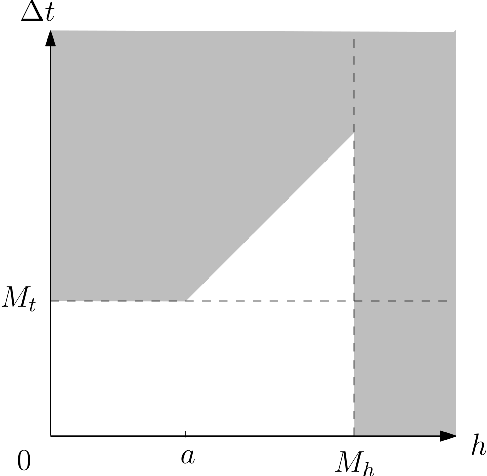
Figure 1: Stability region of a notional quasi-unconditionally stable PDE solver is shown in white; the grey region is the set of $h$ and $\Delta t$ where the method is unstable. In particular, the method is stable in the rectangular region $0<h<M_{h}$, $0<\Delta t<M_{t}$. Notice that outside of this region the method is stable for time steps satisfying certain CFL-like contraints (linear in this illustration). Quasi-unconditional stability does not exclude the possibility of other stability constraints outside of the rectangular region of stability.

As mentioned above, a quasi-unconditionally stable algorithm can be stable even in cases in which the constraints on $(h,\Delta t)$ in Definition 1 are not satisfied, and, in such cases, stability may still take place under certain CFL-like conditions; see Part II for details. Briefly, that reference presents tabular data which display numerically estimated maximum stable values of $\Delta t$ for two- and three-dimensional Navier-Stokes BDF-ADI methods and for a number of spatial-discretization sizes. This data suggests clearly that, for each $s$, maximum stable $\Delta t$ values do approach positive asymptotic limits as finer and finer spatial discretizations are used, as befits a quasi-unconditionally stable scheme.

5 Numerical Implementation

In this section we present details of our full spatio-temporal implementation of the BDF-ADI algorithms discussed above in this text. Spatial discretizations of various kinds can be used in these contexts, including finite-difference, polynomial-spectral and Fourier-continuation [9] discretizations. For the sake of definiteness we restrict our presentation to the Chebyshev-collocation spatial approximation [28, 5] which is briefly reviewed in the following section; results arising from use of the Fourier spectral method [28, 5] are also included in Section 6.

5.1 Chebyshev spatial discretization, GMRES iterations, spectral filtering, geometrical metric terms

Let the computational PDE domain $D=[-1,1]^{3}$ be discretized by means of an $(N+1)$-node Gauss-Lobatto Chebyshev discretization [28, 5] in the $\xi$, $\eta$, and $\zeta$ directions:

$$\xi_{i}=-\cos(\pi i/N_{\xi}) i=0,\dots,N_{\xi},$$ ,

$$\eta_{j}=-\cos(\pi j/N) j=0,\dots,N_{\eta},$$ ,

$$\zeta_{k}=-\cos(\pi k/N) k=0,\dots,N_{\zeta};$$ ,

the treatment for the two-dimensional case is, of course, entirely analogous. In what follows the PDE solution $Q$ is approximated numerically by means of grid discretizations $Q_{ijk}\sim Q(\xi_{i},\eta_{j},\zeta_{k})$ together with the associated Chebyshev expansions

$$Q_{N}(\xi,\eta,\zeta)=\sum_{{\bf 0}\leq(i,j,k)\leq N}\widehat{Q}_{ijk}T_{i}(\xi)T_{j}(\eta)T_{k}(\zeta),$$ (23)

in terms of the Chebyshev polynomials $T_{\ell}$ ($\ell\geq 0$), where $N=(N_{\xi},N_{\eta},N_{\zeta})$, where $\bf 0$ denotes the three-dimensional zero vector, and where inequalities between three-dimensional vectors are interpreted in component-wise fashion. The coefficients $\widehat{Q}_{ijk}$ of the numerical approximation $Q_{N}$ are related to the point values $Q_{ijk}$ by the interpolation relations $Q_{N}(\xi_{i},\eta_{j},\zeta_{k})=Q_{ijk}$ (${\bf 0}\leq(i,j,k)\leq N$).

The discrete Chebyshev spatial differentiation operators we use are standard [28, 5]: the $\xi$-derivative operator $\delta_{\xi}$ applied to a grid function $Q_{ijk}$, for example, is defined as the grid function $(\delta_{\xi}Q)_{ijk}$ whose $(ijk)$ value equals the value of the derivative of the interpolant $Q_{N}$ at the point $(\xi_{i},\eta_{j},\zeta_{k})$:

$$(\delta_{\xi}Q)_{ijk}=\frac{\partial}{\partial\xi}Q_{N}(\xi_{i},\eta_{j},\zeta_{k}).$$ (24)

Similar definitions are used for the operators $\delta_{\xi\xi}$, $\delta_{\eta}$, $\delta_{\eta\eta}$, $\delta_{\xi\eta}=\delta_{\xi}\delta_{\eta}=\delta_{\eta}\delta_{\xi}$ etc. As is common practice, for all of the numerical examples presented in this paper the Chebyshev derivatives are evaluated efficiently by means of the fast cosine transform.

Using the Chebyshev discretizations mentioned above, the one-dimensional boundary value problems given by the ODE systems (18) and the boundary conditions (20) become discrete systems of linear equations. In order to fully take advantage of the fast cosine transform we solve these systems by means of the GMRES iterative solver with second order finite difference preconditioner (cf. [5, p. 293] and [11]); a similar treatment is used in conjunction with Fourier spectral discretizations.

For both Chebyshev and Fourier-spectral discretizations an exponential filter [23], which does not degrade the $s$-th order accuracy of the method (cf. [1, Sec. 4.3]), is employed to ensure stability. In the Chebyshev case, for example, the filtered coefficients $h^{f}_{k}$ for a given function $h=\sum_{k}\widehat{h}_{k}T_{k}(x)$ are given by

$$h^{f}_{k}=\exp\left(-\alpha\left(\frac{k}{N}\right)^{2p}\right)\widehat{h}_{k}.$$

For all of the results presented in this paper we have set $\alpha=16\log 10$ and $p=8$. The filter is applied at the end of the time step to each line of discretization points in each dimension, requiring one fast cosine transform per line to obtain the coefficients $\widehat{h}_{k}$, and one transform to obtain the filtered physical function values.

The transformation of the equations to general coordinates requires the metric terms $\xi_{x}$, $\xi_{y}$, etc; see Section 3.2. The solvers presented in this paper use the so-called “invariant form” of these metric terms [39], but other (accurate) alternatives could be equally advantageous. The derivatives of the physical coordinates ($x_{\xi}$, $x_{\eta}$, etc.) needed in the actual expressions for the metric terms are produced by means of the discrete derivative operators implicit in the Chebyshev or Fourier spatial approximation used in each case.

5.2 Overall algorithmic description and treatment of boundary values and initial time-steps

Given the elements described in previous sections of this paper, our actual implementations of BDF-ADI algorithms of order $s$ can now be described in rather simple terms—except perhaps for some details, which require additional considerations, concerning boundary values of the fluid density and the possible presence of corners and edges in the boundary of the computational domain. The absence of a density boundary condition has previously been successfully addressed by means of discretization strategies based on use of staggered grids see e.g. [12, Ch. 4.6] and the references therein. In some such strategies the velocity and the temperature are collocated on a Gauss-Lobatto grid while the density is collocated on a Gauss grid—so that the density mesh contains no boundary points, and therefore no density boundary conditions are needed. In the context of ADI-based methods such as the ones considered in this paper, however, it is not clear that a natural staggered-grid ADI method could be designed—since the ADI approach requires solution of one-dimensional boundary value problems which couple all field components. An alternative approach is proposed in this paper. This method uses the same Gauss-Lobatto grid for all unknowns, including the density, and therefore it requires determination of the boundary values of the density as part of the overall solution.

Our approach in these regards follows from the following observation: the density components of the unknowns $Q^{*}$, $Q^{**}$ and $Q^{n+1}$ throughout the domain and including the boundary can be obtained by interpreting the corresponding equations (17) (or, equivalently, equations (18)) as a system which includes the density boundary values as unknowns. We demonstrate the method in detail in the case of equation (17a); the treatment of the other equations in either (17) or (18) is analogous. As suggested above, for a fixed pair $(k,\ell)$ we view equation (17a) as a relation between $(d+2)(N-1)+2$ unknowns ($d=3$ in the present example), namely, the discrete values $Q^{*}_{jk\ell}$ of the vector $Q^{*}=((\mathbf{u}^{*})^{\mathrm{T}},T^{*},\rho^{*})^{\mathrm{T}}$ that corresponds to discretization points in the interior of the PDE domain ($1\leq j\leq N-1$) together with the density boundary values ($\rho^{n+1}_{jk\ell}$ for $j=0$ and $j=N$). Clearly, collocation of (17a) at all interior points along the $(k,\ell)$ discretization segment furnishes $(d+2)(N-1)$ equations for these unknowns.

The necessary two additional equations are obtained by enforcing the portion of (17a) that arises from the mass conservation equation at each one of the two boundary points $j=0$ and $j=N$. Note that in order to solve the overall system of $(d+2)(N-1)+2$ equations along the $(k,\ell)$ discretization segment at time $t^{n+1}$, the values of $Q=(\mathbf{u}^{\mathrm{T}},T,\rho)^{\mathrm{T}}$ at the corresponding interior discretization points and boundary points together with the boundary values of $\mathbf{u}$ and $T$ (given by the boundary conditions (20a)) at the boundary points must be available for all time-steps $t^{m}$ with $n-s+1\leq m\leq n$. (For the subsequent equations in (17) or (18) the values of $Q^{*}$ and $Q^{**}$ evaluated in the previous intermediate steps at interior and boundary points are needed as well.) Using such data the algorithm produces the needed interior and boundary values $Q^{*}_{jk\ell}$. As mentioned above, the subsequent equations for the unknowns $Q^{**}$ and $Q^{n+1}$ in (17) or (18) are treated similarly.

It is important to note that in the algorithm just described, the third ADI sweep produces not only the values of the density $\rho^{n+1}$ at the horizontal boundary faces $\zeta=\ell_{1}$ and $\zeta=\ell_{2}$, but also the values of $\rho^{n+1}$ along the vertical boundary faces $\xi=\ell_{1}$, $\xi=\ell_{2}$, $\eta=\ell_{1}$ and $\eta=\ell_{2}$. These are necessary to form the BDF-ADI system (17) at subsequent time-steps. However, as part of the solution along the vertical faces, values for $\mathbf{u}^{n+1}$ and $T^{n+1}$ are also produced, and we have observed that retaining these values for the solution causes a degradation in the order of accuracy (although the solvers continue to enjoy quasi-unconditional stability in this case). Therefore, in order to preserve the order $s$ of time-accuracy, it is important to discard these values of $\mathbf{u}$ and $T$ and substitute them by those given by the boundary conditions (20). This completes the description of the algorithm.

We emphasize that no special boundary conditions are required for either the intermediate density $\rho^{*}$ or the final density $\rho^{n+1}$. The density is determined entirely by equations (18) throughout the domain, up to and including the boundary. Furthermore, the presence of corners does not impact the stability of the solver: no special boundary treatment for the corners of the domain are necessary.

Remark 4.

Although corners in the computational domain do not affect the stability of our solvers, we note that the spatial accuracy may deteriorate as a result of singularities that occur at corners and edges of the computational domain (see e.g. [5, Ch. 6.12] for a corresponding discussion in the context of for spectral discretizations). Provided the physical domain contains no corner or edges, this problem can be eliminated by means of a multi-domain overset decomposition [7, 13], in such a way that actual PDE solutions around corner regions and edge regions in one computational patch are actually replaced by solution values obtained at interior regions in other patches. Actual physical corners and edges, which also give rise to accuracy reductions, can be treated in a variety of ways, but such considerations are beyond the scope of this paper. In any case, the numerical examples in the next section show the correct order of time-accuracy of the solvers with a manufactured solution in a computational domain containing corners and edges, as well as a physical solution in an annular domain—which, of course, contains no corners.

To conclude this section we provide some comments concerning evaluation of solution values at the first $s$ timesteps in a method of overall accuracy order $s$. In the simplest approach the solution is ramped-up from a constant field state (usually zero for all velocities and one for the density and temperature), and the simulation is arranged in such a way that the solution values at each one of the initial $s$ time-steps is known and equal to the assumed constant state. But in some situations evaluation of the transients from given initial conditions may need to be obtained; see e.g. the example provided in Section 6 involving flow in an annulus, where the density has a non-constant initial condition. Use of explicit solvers is some times recommended to obtain the first few solution values, but such explicit solvers generally require use of significantly smaller time-steps than those used by the implicit solver—in view of their inherent properties of conditional stability. Furthermore, a high order multi-step explicit solver would also require previous time levels, and a Runge-Kutta method requires special treatment of boundary conditions for the intermediate stages. In order to avoid such difficulties, we propose a strategy based on use of the first-order BDF-ADI method followed by Richardson-extrapolation (cf. [32] and references therein) of a sufficiently high order so as to match the overall order of time-accuracy of the method. For example, to produce a second-order accurate solution at $t=\Delta t$ from initial data $Q^{0}$, two solutions using the first-order BDF-ADI algorithm are computed at time $t=\Delta t$—one solution ($Q^{1}_{(1)}$) with time step equal to $\Delta t$, the other ($Q^{1}_{(2)}$) with time-step $\Delta t/2$. The second-order accurate solution $Q^{1}$ is obtained as an appropriate linear combination of $Q^{1}_{(1)}$ and $Q^{2}_{(2)}$: $Q^{1}=2Q^{1}_{(2)}-Q^{1}_{(1)}.$

6 Numerical Results

This section presents a variety of numerical results produced by the BDF-ADI solvers introduced in this paper for two- and three-dimensional spatial domains and for orders $s$ with $2\leq s\leq 6$. In particular, these results demonstrate that the proposed solvers do enjoy the claimed spatial and temporal orders of accuracy and general applicability; detailed studies demonstrating the claimed stability properties are deferred to Part II. All of the numerical examples were obtained from runs on either a single core of an Intel i5-2520M processor with 4 GB of memory, or a single core of an Intel Xeon X5650 processor with 24 GB of memory. Unless otherwise indicated, all simulations use the parameter values $\mathrm{Pr}=0.71$ and $\gamma=1.4$, and the (non-dimensional) viscosity and thermal conductivity are given by Sutherland’s law (2) with $S_{\kappa}=S_{\mu}=0.3$.

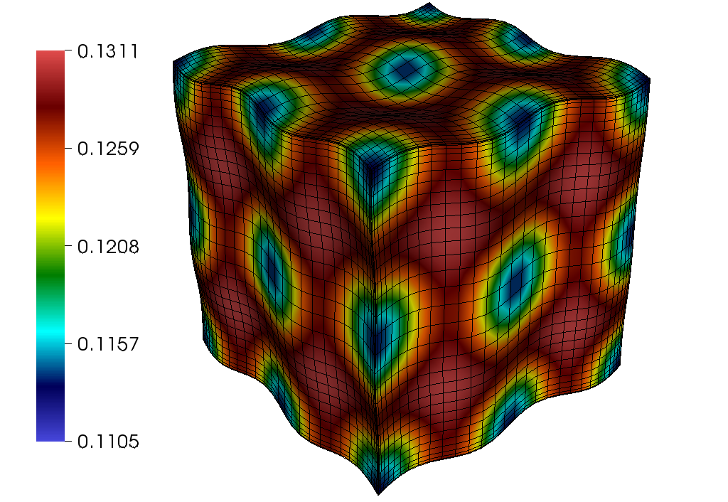
Figure 2: The wavy cube used in the convergence tests of the three-dimensional solver. The coloring corresponds to the Jacobian of transformation.

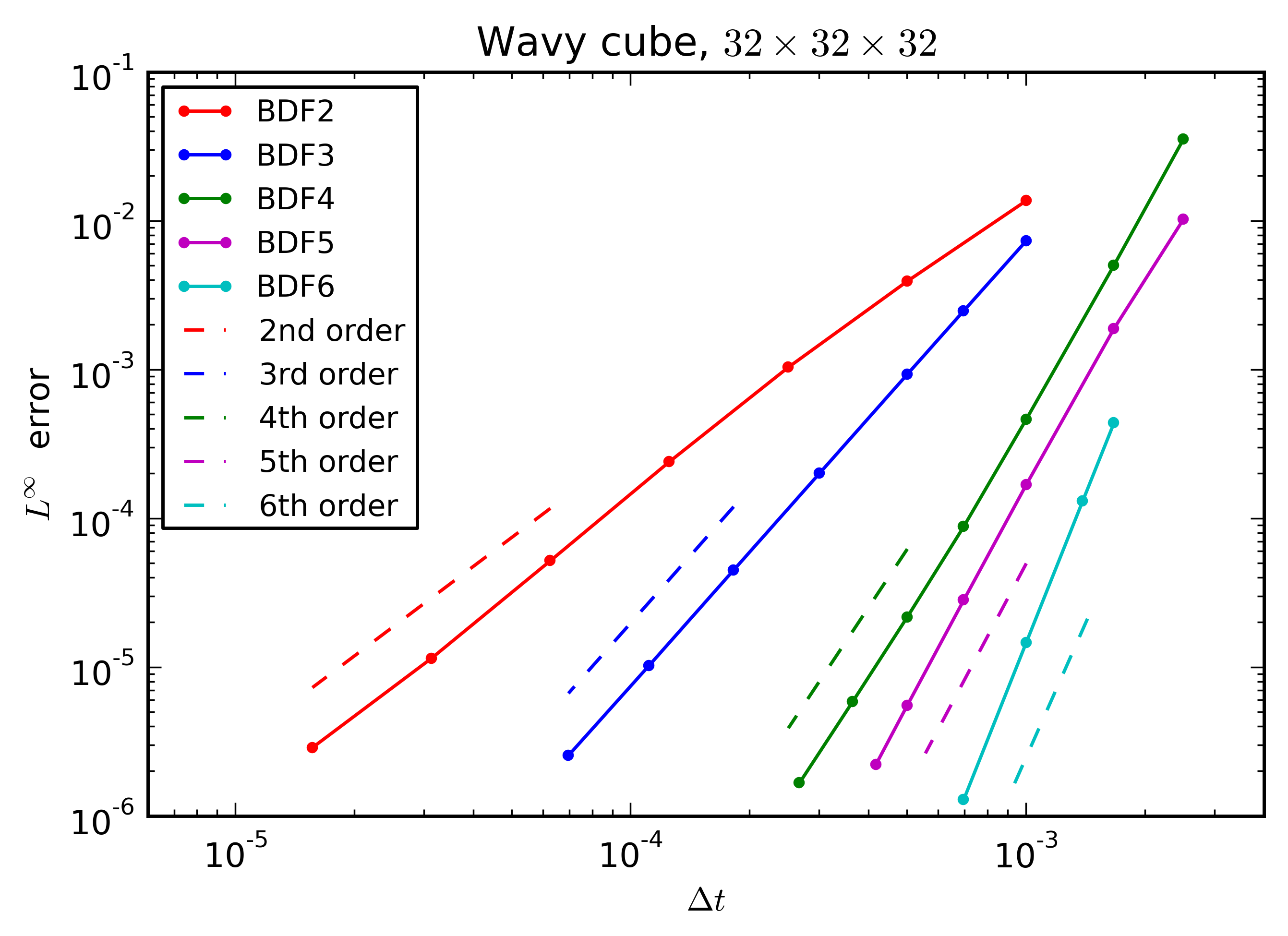
Figure 3: Convergence of the three-dimensional BDF-ADI solvers of orders $s$, $s=2,\dots,6$, for the Navier-Stokes problem in the wavy cube.

$Q_{j}$	$\alpha_{j}$	$\beta_{j}$	$\lambda_{j}$	$\phi_{j,t}$	$\phi_{j,\xi}$	$\phi_{j,\eta}$	$\phi_{j,\zeta}$
$u$	0	1	25	-1	0	0	0
$v$	0	1	25	-2	0	0	0
$w$	0	1	25	-3	0	0	0
$\rho$	1	0.2	25	-4	4	7	14
$T$	1	0.2	25	-5	5	6	15

Table 3: Parameters used for the 3D manufactured solution.

Using the method of manufactured solutions (MMS) our first set of examples demonstrates that the proposed solvers achieve the expected temporal order of convergence. According to the MMS strategy, an arbitrary solution $Q$ is prescribed, and a source term is added to the right hand side of equation (3.2) in such a way that the proposed solution actually satisfies the equation. For this set of examples we use the MMS solution

$$Q_{j}(\xi,\eta,\zeta,t)=\alpha_{j}+\beta_{j}\sin(2\pi\lambda_{j}t+\phi_{j,t})\sin(2\pi\xi+\phi_{j,\xi})\sin(2\pi\eta+\phi_{j,\eta})\sin(2\pi\zeta+\phi_{j,\zeta})$$

where $Q_{j}$ is the $j$th component of the solution vector and where the various $\alpha_{j}$, $\beta_{j}$, $\lambda_{j}$, $\phi_{j,\cdot}$ are constants. The parameter values we use for the solution are given in Table 3. The test geometry in this context is a “wavy cube” given by the equations

$$x(\xi,\eta,\zeta) = \xi+a\left(\sin(2\pi n\eta)+\sin(2\pi n\zeta)\right)$$

$$y(\xi,\eta,\zeta) = \eta+a\left(\sin(2\pi n\xi)+\sin(2\pi n\zeta)\right)$$

$$z(\xi,\eta,\zeta) = \zeta+a\left(\sin(2\pi n\xi)+\sin(2\pi n\eta)\right)$$

with $a=0.015$, $n=2$, and with $0\leq\xi,\eta,\zeta\leq 1$, which is illustrated in Figure 2. Only the velocity components ($\mathbf{u}=0$) and temperature $T$ are prescribed at the boundary according to the manufactured solution; the boundary values of the density are obtained from the solution process, as described in Section 5.2. The Reynolds number and Mach number in these examples are taken to equal $\mathrm{Re}=10^{3}$ and $\mathrm{Ma}=0.85$. The second- through sixth-order convergence of the methods is demonstrated in Figure 3. Note in particular that the manufactured $T$ and $\rho$ solutions are time-dependent on the boundary of the domain, thus demonstrating, in particular, that the proposed numerical boundary condition implementation preserves the correct order of time-accuracy even under time-varying boundary values.

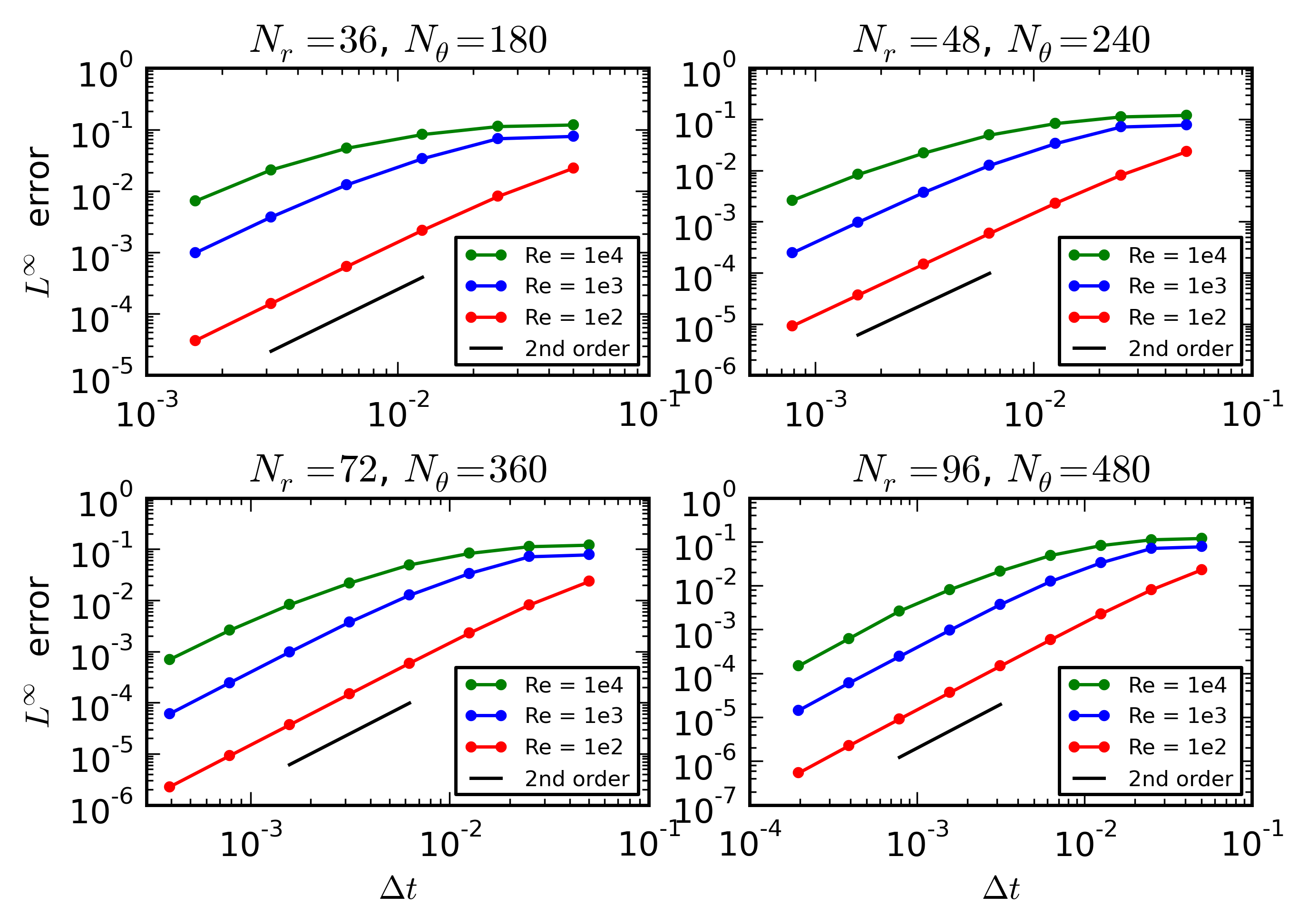
Figure 4: Convergence of the BDF2-ADI solver in an annulus for various mesh discretizations and Reynolds numbers.

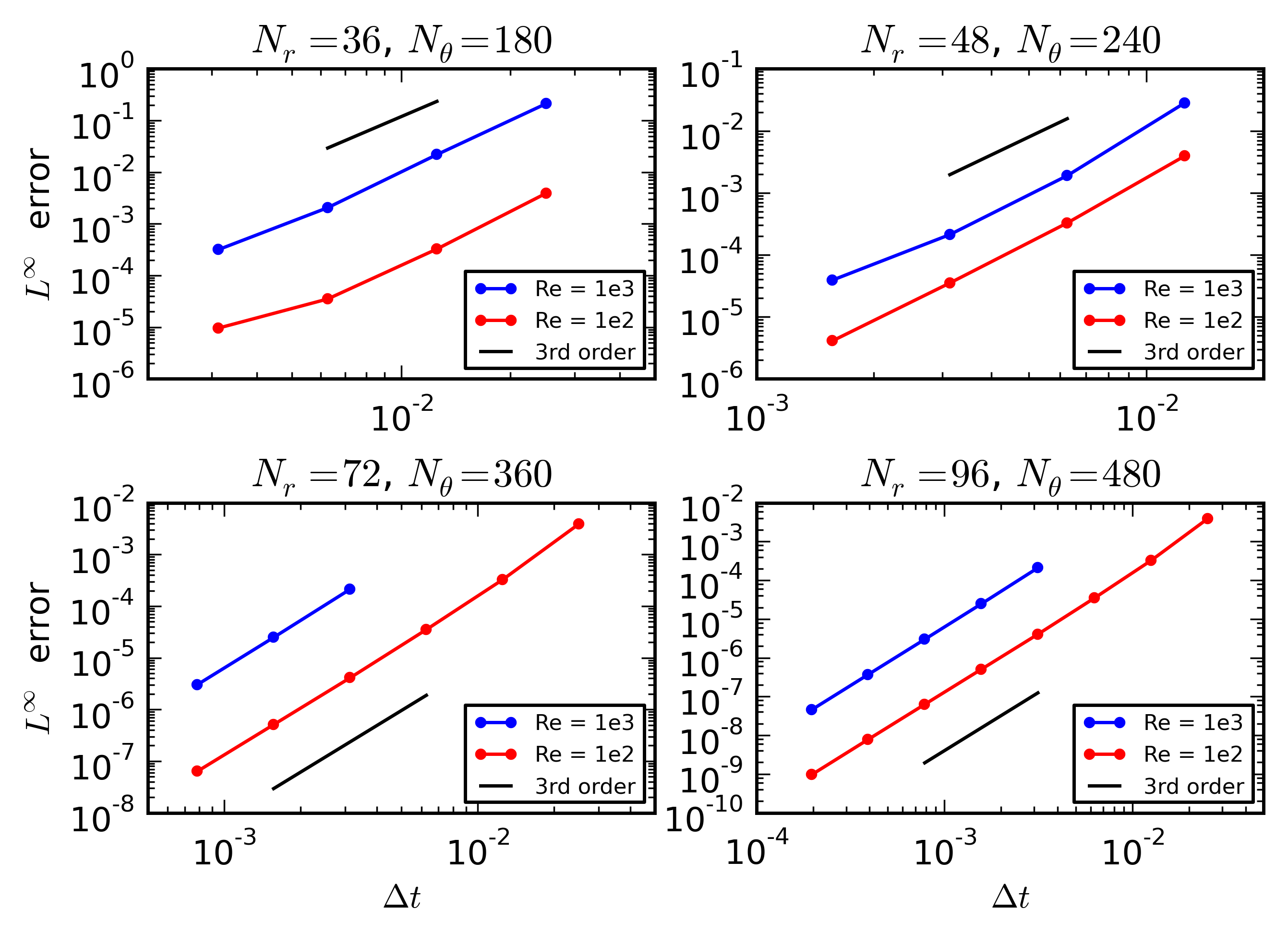
Figure 5: Convergence of the BDF3-ADI solver in an annulus with various mesh discretizations and Reynolds numbers.

Next, we demonstrate the convergence of the solver in two-dimensions with a physical flow example at $\texttt{Ma}=0.8$ in an annulus with inner radius $0.1$ and outer radius $0.5$ using Chebyshev collocation in the radial direction and Fourier collocation in the azimuthal direction. The flow starts with a zero initial condition for all fields except temperature and density; the initial conditions for the former are taken to equal $1.0$, while for the latter the initial conditions are taken to equal the sum of the scalar $1.0$ plus two Gaussian functions of the form

$$a\exp\left(-\frac{(x-x_{0})^{2}+(y-y0)^{2}}{2\sigma^{2}}\right)$$ (25)

with parameters $a=0.3$, $\sigma=0.1$, $x_{0}=-0.2$, $y_{0}=0.2$ and $a=-0.2$, $\sigma=0.07$, $x_{0}=0.2$, $y_{0}=0$, respectively. For time between $t=0$ and $t=0.5$, the rotation of the inner cylinder is ramped up smoothly until it reaches a tangential velocity of $1.0$. A temperature source term equal to ($\sin(2\pi t)$ times a Gaussian in space given by equation (25) with $a=2.5$, $\sigma=0.05$, $x_{0}=-0.2$, $y_{0}=-0.2$) is also used. The convergence of the solver at time $t=1.0$ is estimated via comparison with the solution obtained from a fine discretization ($N_{r}=108$, $N_{\theta}=540$, $\Delta t=0.1\times 2^{-10}$). Figures  4 and  5 verify the expected rates of convergence at various Reynolds numbers.

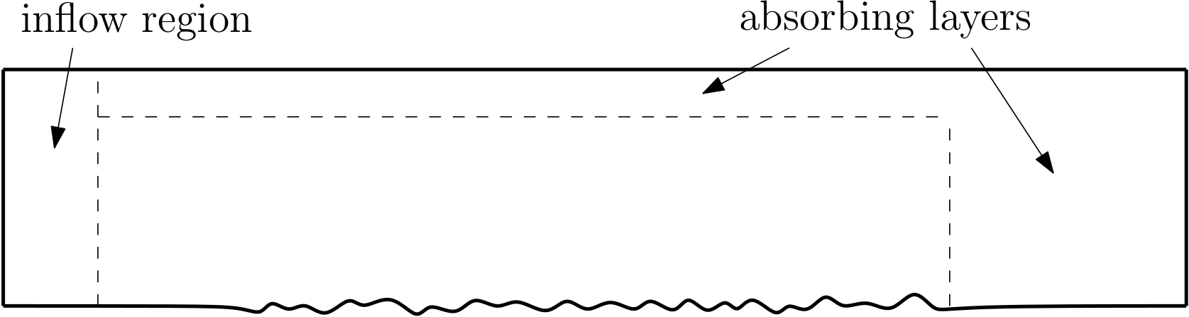
Figure 6: Schematic set-up of unsteady flow over a bumpy plate (not to scale).

$\begin{array}[]{c}\includegraphics[width=375.80542pt]{bumpyPlate9760}\\ \includegraphics[width=375.80542pt]{bumpyPlate9820}\\ \includegraphics[width=375.80542pt]{bumpyPlate9880}\\ \includegraphics[width=375.80542pt]{bumpyPlate9940}\end{array}$

Figure 7: Evolution of the $y$-velocity component in two-dimensional boundary layer flow over a bumpy plate. From top to bottom, the solution times for the figures are $t=9.76,\;9.82,\;9.88,\;9.94$.

Next, a demonstration of boundary layer flow over a “bumpy” plate in 2D at high Reynolds number is presented. Here the domain is such that the left and right edges of the domain lie on the lines $x=x_{\ell}=1$ and $x=x_{r}=4$, while the top and bottom boundaries lie on the curves $y_{t}=0.2$ and

$$y_{b}(x)=\exp\left(-\left(\frac{x-2.5}{1.2}\right)^{12}\right)\sum_{m=1}^{4}a_{m}\sin(c_{m}x),$$

respectively, where $a_{1}=5\times 10^{-4}$, $a_{2}=8\times 10^{-4}$, $a_{3}=6\times 10^{-4}$, $a_{4}=4\times 10^{-4}$, $c_{1}=300$, $c_{2}=207$, $c_{3}=161$ and $c_{4}=124$. The mesh in the interior of the domain is generated by means of transfinite interpolation [22]. A schematic illustration of the set-up is provided in Figure 6. A total of 1536 (resp. 96) Chebyshev collocation points were used in the horizontal (resp. vertical) direction .

To initialize the flow and impose boundary conditions we use the asymptotic solution provided by the boundary layer equations for the present compressible-flow configuration [42, Ch. 7]. Here we provide a brief overview in these regards; a more detailed discussion can be found, e.g., in the aforementioned reference. For simplicity in the solution of boundary-layer approximate equation we assume that the viscosity and thermal conductivity are linear functions of temperature ($\mu(T)=\kappa(T)=T$), and that the Prandtl number equals unity: $\mathrm{Pr}=1$. Using $x$ and $y$ coordinates tangent and normal to the infinite planar boundary, the free-stream solution values as $y\to\infty$ are assumed to equal $u_{\infty}=1$, $v_{\infty}=0$, $T_{\infty}=1$ and $\rho_{\infty}=1$. The boundary layer equations are obtained by transforming the steady ($Q_{t}=0$) two-dimensional Navier-Stokes equations by means of the change of variables $y=\delta Y$, where $\delta=\mathrm{Re}^{1/2}$ is the characteristic length scale of the boundary layer. Furthermore, the solution components are assumed to be perturbations of the free-stream values of the form $u=u_{\infty}+\delta u_{1}$, $v=\delta v_{1}$, $T=T_{\infty}+\delta T_{1}$, $\rho=\rho_{\infty}+\delta\rho_{1}$, which leads to a set of equations for the inner solutions (terms with subscript 1). Using the similarity variable $\bar{\eta}=\bar{\eta}(x^{-1/2}Y)$ together with the Howarth transformation [25], we obtain the following simplified set of equations for $\bar{\eta}$, $u_{1}$, $v_{1}$, $\rho_{1}$, and $T_{1}$ as functions of $x$ and $Y$:

$$\frac{\partial}{\partial Y}\bar{\eta}=\rho_{1},$$

$$\rho_{1}\,u_{1}=f^{\prime}(\bar{\eta}),$$

$$\rho_{1}\,v_{1}=\frac{1}{2}x^{-1/2}\left(\bar{\eta}\,f^{\prime}(\bar{\eta})-f(\bar{\eta})\right),$$

$$T_{1}=u_{1}+T_{\mathrm{wall}}(1-u_{1})+\frac{1}{2}(\gamma-1)\mathrm{Ma}^{2}(u_{1}-u_{1}^{2}),$$

$$\rho_{1}T_{1}=1,$$

where $T_{\mathrm{wall}}$ is the temperature at the wall and $f$ is the solution of the Blasius equation

$$f^{\prime\prime\prime}+\frac{1}{2}f\,f^{\prime}=0,$$

$$f(0)=f^{\prime}(0)=0,$$

$$f^{\prime}(\eta)\rightarrow 1\;\mathrm{as}\;\eta\rightarrow\infty.$$

The similarity variable $\bar{\eta}$ is obtained by eliminating the other unknowns and using a Newton-Kantorovich iterative solver [5, App. C] with initial guess computed by standard fourth order Runge-Kutta. The remaining unknowns can then be obtained explicitly from the above relations. The resulting solution $Q_{\mathrm{ref}}$ of the boundary layer equations is used to provide the initial condition and boundary conditions at inflow and, as discussed in what follows, in the absorbing layers of the computational domain as well.

The boundary conditions for this example are no-slip conditions on the bottom boundary ($\mathbf{u}_{\mathrm{wall}}=0$ and $T_{\mathrm{wall}}=1$), an absorbing layer of thickness 0.05 at the top of the domain, another absorbing layer of thickness 0.5 is on the right, and inflow conditions in a region of thickness 0.1 on the left; cf. Figure 6. For each absorbing layer, a term of the form $\sigma(\xi,\eta)Q_{\mathrm{ref}}$ is added to the right hand side of the PDE (3.2) and $\sigma I$ is added to the matrix $M^{0}$, where $I$ is the identity (cf. the related, more elaborate absorbing-layer method [2]). The variable coefficient $\sigma$ is given by

$$\sigma(\xi,\eta)=A\left(1-\psi\left(\frac{d(\xi,\eta)}{L}\right)\right)$$ (26)

where $A$ is the absorption factor, $L$ is the width of the layer, $d(\xi,\eta)$ is the distance to the boundary in question, and the function $\psi$ is given by

$$\psi(x)=\begin{cases}0&,x\leq 0\\ 1&,x\geq 1\\ \left[1+\exp\left(\frac{1}{x}-\frac{1}{1-x}\right)\right]^{-1}&,0<x<1\end{cases}$$ (27)

For the top boundary we use $A=50$, $L=0.05$ and for the right boundary we use $A=20$, $L=0.5$; these selections enforce adequate damping in the absorbing layers. The boundary layer solution $Q_{\mathrm{ref}}$ is prescribed in the inflow region for all times. Figure 7 displays the $y$-velocity component for various times, with $\mathrm{Re}=10^{6}$, $\mathrm{Ma}=0.85$, and $\Delta t=10^{-3}$. With this discretization ($\Delta x_{\min}=3.1\times 10^{-6}$ and $\Delta y_{\min}=5.4\times 10^{-5}$), an explicit solver would require a significantly smaller time step for stability.

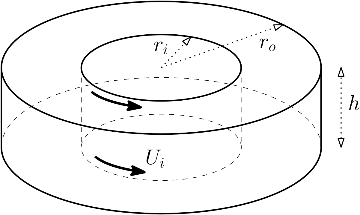
Figure 8: Geometry of the Taylor-Couette flow example. The fluid is confined in the region between the cylinders of radii $r_{i}$ and $r_{o}$ and between two planes separated by a distance $h$. The inner cylinder rotates with speed $U_{i}$ while all other boundaries remain stationary.

$\begin{array}[]{c|c|c}\includegraphics[width=140.92792pt]{TCTwoCellU}&\includegraphics[width=140.92792pt]{TCTwoCellW}&\includegraphics[width=140.92792pt]{TCTwoCellVort}\\ \includegraphics[width=140.92792pt]{TCOneCellU}&\includegraphics[width=140.92792pt]{TCOneCellW}&\includegraphics[width=140.92792pt]{TCOneCellVort}\end{array}$

Figure 9: Profiles of the (a) azimuthal velocity, (b) vertical velocity and (c) azimuthal component of vorticity in small-aspect-ratio Taylor-Couette flow at $\mathrm{Ma}=0.2$ and $\mathrm{Re}=700$. The top (resp. bottom) row displays profiles associated with the two-cell (resp. one-cell) stable mode.

Our next example concerns three-dimensional simulations of Taylor-Couette flow, that is to say, flow of a fluid between two concentric rotating cylinders, as depicted in Figure 8. Most studies of Taylor-Couette flow deal with incompressible fluids, but the dynamics for subsonic compressible gases are similar, as shown in [33, 26]. The geometry is defined by the inner radius $r_{i}$, outer radius $r_{o}$ and height $h$. In what follows, we consider only the case where the inner cylinder rotates and the outer cylinder together with the top and bottom walls are stationary. In this case, the Reynolds number $\mathrm{Re}$ is defined with respect to the velocity of the inner cylinder.

The small aspect ratio regime ($\Gamma=\frac{h}{r_{o}-r_{i}}\approx 1$ or less) has been extensively studied both numerically and experimentally (in the incompressible case)—in part because of the property that two or more stable flows can exist for the same values of the system parameters $\Gamma$, $\mathrm{Re}$, $r_{o}$, $r_{i}$ [36, 34]. The incompressible solution is reported [36, 34] to behave as follows: For $\Gamma=1$ and radius ratio $r_{i}/r_{o}=0.5$, there is only one stable flow at small $\mathrm{Re}$, which is characterized by two axisymmetric toroidal vortices, one on top of the other, similar to those depicted in the upper image in Figure  9 (c). At about $\mathrm{Re}\approx 133$, this mode becomes unstable. The stable mode is then characterized by a single large axisymmetric toroidal vortex in the center and a smaller one in the inner upper corner, similar to those shown in the lower image in Figure 9 (c). Both modes are stable in the range $603\lesssim\mathrm{Re}\lesssim 786$.

Starting from the same initial condition (zero velocity, density and temperature equal to $1.0$) and ending at the same final inner cylinder rotational velocity with $\mathrm{Re}=700$ and $\mathrm{Ma}=0.2$, our simulations produce both stable modes. To produce the first mode, the inner cylinder velocity was varied as a function of time according to

$$U_{i}(t)=\psi\left(\frac{t}{160}\right)$$

where $\psi$ is defined in (27). To produce the second mode, in turn, the cylinder velocity was varied according to the relation

$$U_{i}(t)=0.4\psi\left(\frac{t}{10}\right)+0.6\psi\left(\frac{t-150}{150}\right).$$

The spatial discretization used a total of 48 Chebyshev collocation points in the radial and $z$ directions and 64 Fourier collocation points in the azimuthal direction. No-slip isothermal ($T=1$) boundary conditions were used on all walls, with the angular velocity at the top and bottom boundaries prescribed as

$$u_{\theta}(r,t)=\exp\left(-\left(2\sqrt{\mathrm{Re}}(r-r_{i})\right)^{2}\right)U_{i}(t).$$

The time discretization for both simulations was set at $\Delta t=0.02$ and simulations were stopped at $t=400$. At $\mathrm{Ma}=0.2$, there is less than 0.5% deviation in the density from the initial condition $\rho=T=1$ throughout the simulations. The presence of corners in the geometry undoubtedly gives rise to reductions in the solution accuracy (cf. Remark 4); nevertheless, Figure 9 shows both modes at $t=300$, which compares well to the experimental and numerical results in the literature for the incompressible case [36, 34]—as it should given the low value of the Mach number considered.

7 Conclusions

This paper introduced an implicit solution strategy for the compressible Navier-Stokes equations which enjoys high-order accuracy in time and which runs at spatial FFT speeds per time-step; of course, the proposed BDF-ADI strategy can also be used in conjunction with other spectral or non-spectral spatial approximations (such as finite-differences, Fourier-Continuation, etc.). As emphasized above in this text, the algorithms presented in this paper are the first ADI-based Navier-Stokes solvers for which second order or better accuracy has been verified in practice under non-trivial (non-periodic) boundary conditions. The numerical examples presented in this contribution demonstrate the favorable qualities inherent in the proposed algorithms in both space and time.

Acknowledgments

The authors gratefully acknowledge support from the Air Force Office of Scientific Research and the National Science Foundation. MC also thanks the National Physical Science Consortium for their support of this effort.

Appendix A Quasilinear-like matrix coefficients in Cartesian and curvilinear coordinates

Let $a=\frac{1}{\mathrm{Re}}\frac{\mu^{\prime}(T)}{\rho}$, $b=\frac{\gamma(\gamma-1)\mathrm{Ma}^{2}}{\mathrm{Re}}\frac{\mu(T)}{\rho}$, $c=\frac{\gamma}{\mathrm{Re}\mathrm{Pr}}\frac{\kappa^{\prime}(T)}{\rho}$, $d=\frac{1}{\gamma\mathrm{Ma}^{2}}$, and $e=\gamma-1$. The coefficient matrices for Navier-Stokes equations in quasilinear-like Cartesian form (3.1) are

$$M^{x}=\begin{pmatrix}u-\frac{2}{3}aT_{x}&-\frac{1}{2}aT_{y}&-\frac{1}{2}aT_{z}&d-a\left(u_{x}-\frac{1}{3}\nabla\cdot\mathbf{u}\right)&d\frac{T}{\rho}\\[6.45831pt] \frac{1}{3}aT_{y}&u-\frac{1}{2}aT_{x}&0&-\frac{1}{2}a(v_{x}+u_{y})&0\\[6.45831pt] \frac{1}{3}aT_{z}&0&u-\frac{1}{2}aT_{x}&-\frac{1}{2}a(w_{x}+u_{z})&0\\[6.45831pt] eT-b\left(2u_{x}-\frac{2}{3}\nabla\cdot\mathbf{u}\right)&-b(v_{x}+u_{y})&-b(w_{x}+u_{z})&u-cT_{x}&0\\[6.45831pt] \rho&0&0&0&u\par\end{pmatrix}$$

$$M^{y}=\begin{pmatrix}v-\frac{1}{2}aT_{y}&\frac{1}{3}aT_{x}&0&-\frac{1}{2}a(v_{x}+u_{y})&0\\[6.45831pt] -\frac{1}{2}aT_{x}&v-\frac{2}{3}aT_{y}&-\frac{1}{2}aT_{z}&d-a\left(v_{y}-\frac{1}{3}\nabla\cdot\mathbf{u}\right)&d\frac{T}{\rho}\\[6.45831pt] 0&\frac{1}{3}aT_{z}&v-\frac{1}{2}aT_{y}&-\frac{1}{2}a(w_{y}+v_{z})&0\\[6.45831pt] -b(v_{x}+u_{y})&eT-b\left(2v_{y}-\frac{2}{3}\nabla\cdot\mathbf{u}\right)&-b(w_{y}+v_{z})&v-cT_{y}&0\\[6.45831pt] 0&\rho&0&0&v\par\end{pmatrix}$$

$$M^{z}=\begin{pmatrix}w-\frac{1}{2}aT_{z}&0&\frac{1}{3}aT_{x}&-\frac{1}{2}a(w_{x}+u_{z})&0\\[6.45831pt] 0&w-\frac{1}{2}aT_{z}&\frac{1}{3}aT_{y}&-\frac{1}{2}a(w_{y}+v_{z})&0\\[6.45831pt] -\frac{1}{2}aT_{x}&-\frac{1}{2}aT_{y}&w-\frac{2}{3}aT_{z}&d-a\left(w_{z}-\frac{1}{3}\nabla\cdot\mathbf{u}\right)&d\frac{T}{\rho}\\[6.45831pt] -b(w_{x}+u_{z})&-b(w_{y}+v_{z})&eT-b\left(2w_{z}-\frac{2}{3}\nabla\cdot\mathbf{u}\right)&w-cT_{z}&0\\[6.45831pt] 0&0&\rho&0&w\par\end{pmatrix}$$

$$M^{xx}=-\frac{1}{\mathrm{Re}\,\rho}\;\mathrm{diag}\left(\frac{4}{3}\mu,\;\mu,\;\mu,\;\frac{\gamma}{\mathrm{Pr}}\kappa,\;0\right)$$

$$M^{yy}=-\frac{1}{\mathrm{Re}\,\rho}\;\mathrm{diag}\left(\mu,\;\frac{4}{3}\mu,\;\mu,\;\frac{\gamma}{\mathrm{Pr}}\kappa,\;0\right)$$

$$M^{zz}=-\frac{1}{\mathrm{Re}\,\rho}\;\mathrm{diag}\left(\mu,\;\mu,\;\frac{4}{3}\mu,\;\frac{\gamma}{\mathrm{Pr}}\kappa,\;0\right)$$

The matrices $M^{xy}$, $M^{xz}$ and $M^{yz}$ are zero except for two elements each, which are

$$M^{xy}_{u,v}=M^{xy}_{v,u}=M^{xz}_{u,w}=M^{xz}_{w,u}=M^{yz}_{v,w}=M^{yz}_{w,v}=-\frac{1}{3}\frac{1}{\mathrm{Re}}\frac{\mu}{\rho},$$

Using the above definitions and the metric terms $\xi_{x}$, $\xi_{y}$, etc. the coefficient matrices in general coordinates for use in (3.2) are computed as

$$M^{\xi}=\xi_{x}M^{x}+\xi_{y}M^{y}+\xi_{z}M^{z}+\xi_{xx}M^{xx}+\xi_{yy}M^{yy}+\xi_{zz}M^{zz}+\xi_{xy}M^{xy}+\xi_{xz}M^{xz}+\xi_{yz}M^{yz}$$

$$M^{\xi\xi}=\xi_{x}^{2}M^{xx}+\xi_{y}^{2}M^{yy}+\xi_{z}^{2}M^{zz}+\xi_{x}\xi_{y}M^{xy}+\xi_{x}\xi_{z}M^{xz}+\xi_{y}\xi_{z}M^{yz}$$

and $M^{\eta}$, $M^{\eta\eta}$ ($M^{\zeta}$, $M^{\zeta\zeta}$) are obtained by replacing $\xi$ with $\eta$ ($\zeta$) in the above equations. The mixed derivative matrices are computed as

$$M^{\xi\eta}=\xi_{x}\eta_{x}M^{xx}+\xi_{y}\eta_{y}M^{yy}+\xi_{z}\eta_{z}M^{zz}+(\xi_{x}\eta_{y}+\eta_{x}\xi_{y})M^{xy}+(\xi_{x}\eta_{z}+\eta_{x}\xi_{z})M^{xz}+(\xi_{y}\eta_{z}+\eta_{y}\xi_{z})M^{yz}$$

$$M^{\xi\zeta}=\xi_{x}\zeta_{x}M^{xx}+\xi_{y}\zeta_{y}M^{yy}+\xi_{z}\zeta_{z}M^{zz}+(\xi_{x}\zeta_{y}+\zeta_{x}\xi_{y})M^{xy}+(\xi_{x}\zeta_{z}+\zeta_{x}\xi_{z})M^{xz}+(\xi_{y}\zeta_{z}+\zeta_{y}\xi_{z})M^{yz}$$

$$M^{\eta\zeta}=\eta_{x}\zeta_{x}M^{xx}+\eta_{y}\zeta_{y}M^{yy}+\eta_{z}\zeta_{z}M^{zz}+(\eta_{x}\zeta_{y}+\zeta_{x}\eta_{y})M^{xy}+(\eta_{x}\zeta_{z}+\zeta_{x}\eta_{z})M^{xz}+(\eta_{y}\zeta_{z}+\zeta_{y}\eta_{z})M^{yz}.$$

References

- [1] N. Albin and O. P. Bruno. A spectral FC solver for the compressible Navier–Stokes equations in general domains I: Explicit time-stepping. Journal of Computational Physics, 230(16):6248–6270, July 2011.
- [2] D. Appelö and T. Colonius. A high-order super-grid-scale absorbing layer and its application to linear hyperbolic systems. Journal of Computational Physics, 228(11):4200–4217, 2009.
- [3] R. M. Beam and R. Warming. An implicit factored scheme for the compressible Navier-Stokes equations. AIAA journal, 16(4):393–402, 1978.
- [4] R. M. Beam and R. F. Warming. An implicit finite-difference algorithm for hyperbolic systems in conservation-law form. Journal of Computational Physics, 22(1):87–110, Sept. 1976.
- [5] J. P. Boyd. Chebyshev and Fourier spectral methods. Courier Dover Publications, 2001.
- [6] W. R. Briley and H. McDonald. On the structure and use of linearized block implicit schemes. Journal of Computational Physics, 34(1):54–73, Jan. 1980.
- [7] D. L. Brown, W. D. Henshaw, and D. J. Quinlan. Overture: Object-oriented tools for overset grid applications. AIAA paper No. 99, 9130, 1999.
- [8] O. P. Bruno and M. Cubillos. On the quasi-unconditional stability of BDF-ADI solvers for the compressible Navier-Stokes equations. 2015.
- [9] O. P. Bruno and E. Jimenez. Higher-order linear-time unconditionally stable alternating direction implicit methods for nonlinear convection-diffusion partial differential equation systems. Journal of Fluids Engineering, 136(6):060904–060904, Apr. 2014.
- [10] O. P. Bruno and M. Lyon. High-order unconditionally stable FC-AD solvers for general smooth domains I. Basic elements. Journal of Computational Physics, 229(6):2009–2033, Mar. 2010.
- [11] O. P. Bruno and A. Prieto. Spatially dispersionless, unconditionally stable FC–AD solvers for variable-coefficient PDEs. Journal of Scientific Computing, 58(2):331–366, 2014.
- [12] C. Canuto, M. Y. Hussaini, A. Quarteroni, and T. A. Zang. Spectral methods: evolution to complex geometries and applications to fluid dynamics. Springer Science & Business Media, June 2007.
- [13] M. Cubillos. General-domain compressible Navier-Stokes solvers exhibiting quasi-unconditional stability and high-order accuracy in space and time. PhD, California Institute of Technology, Mar. 2015.
- [14] G. G. Dahlquist. A special stability problem for linear multistep methods. BIT Numerical Mathematics, 3(1):27–43, Mar. 1963.
- [15] J. Douglas and J. E. Gunn. Two high-order correct difference analogues for the equation of multidimensional heat flow. Mathematics of Computation, 17(81):71–80, 1963.
- [16] J. Douglas, Jr. and J. E. Gunn. Alternating direction methods for parabolic systems in M space variables. J. ACM, 9(4):450–456, Oct. 1962.
- [17] J. Douglas Jr. and J. E. Gunn. A general formulation of alternating direction methods. Numerische Mathematik, 6(1):428–453, Dec. 1964.
- [18] J. A. Ekaterinaris. Implicit, high-resolution, compact schemes for gas dynamics and aeroacoustics. Journal of Computational Physics, 156(2):272–299, Dec. 1999.
- [19] E. Garnier, N. Adams, and P. Sagaut. Large eddy simulation for compressible flows. Springer, 2009.
- [20] G. H. Golub and C. F. Van Loan. Matrix computations, volume 3. JHU Press, 2012.
- [21] R. E. Gordnier. High fidelity computational simulation of a membrane wing airfoil. Journal of Fluids and Structures, 25(5):897–917, July 2009.
- [22] W. J. Gordon and C. A. Hall. Construction of curvilinear co-ordinate systems and applications to mesh generation. International Journal for Numerical Methods in Engineering, 7(4):461–477, 1973.
- [23] D. Gottlieb and C.-W. Shu. On the Gibbs phenomenon and its resolution. SIAM Review, 39(4):644–668, 1997.
- [24] K. A. Hoffmann and S. T. Chiang. Computational fluid dynamics, vol. 2. Engineering Education System, Wichita, Kansas, pages 21–46, 2000.
- [25] L. Howarth. Concerning the effect of compressibility on laminar boundary layers and their separation. Proceedings of the Royal Society of London. Series A. Mathematical and Physical Sciences, 194(1036):16–42, July 1948.
- [26] K.-H. Kao and C.-Y. Chow. Linear stability of compressible Taylor–Couette flow. Physics of Fluids A: Fluid Dynamics (1989-1993), 4(5):984–996, May 1992.
- [27] S. Kawai and S. K. Lele. Large-eddy simulation of jet mixing in supersonic crossflows. AIAA Journal, 48(9):2063–2083, 2010.
- [28] D. A. Kopriva. Implementing spectral methods for partial differential equations: Algorithms for scientists and engineers. Springer Science & Business Media, 2009.
- [29] J. D. Lambert. Numerical methods for ordinary differential systems: the initial value problem. John Wiley & Sons, Inc., 1991.
- [30] R. LeVeque. Finite difference methods for ordinary and partial differential equations. Society for Industrial and Applied Mathematics, Jan. 2007.
- [31] R. J. Leveque. Intermediate boundary conditions for LOD, ADI and approximate factorization methods. Technical Report NASA-CR-172591, ICASE-85-21, NASA, Mar. 1985.
- [32] M. Lyon and O. P. Bruno. High-order unconditionally stable FC-AD solvers for general smooth domains II. Elliptic, parabolic and hyperbolic PDEs; theoretical considerations. Journal of Computational Physics, 229(9):3358–3381, May 2010.
- [33] A. Manela and I. Frankel. On the compressible Taylor–Couette problem. Journal of Fluid Mechanics, 588:59–74, 2007.
- [34] F. Marques and J. M. Lopez. Onset of three-dimensional unsteady states in small-aspect-ratio Taylor–Couette flow. Journal of Fluid Mechanics, 561:255–277, 2006.
- [35] D. W. Peaceman and H. H. Rachford, Jr. The numerical solution of parabolic and elliptic differential equations. Journal of the Society for Industrial and Applied Mathematics, 3(1):28–41, Mar. 1955.
- [36] G. Pfister, H. Schmidt, K. A. Cliffe, and T. Mullin. Bifurcation phenomena in Taylor-Couette flow in a very short annulus. Journal of Fluid Mechanics, 191:1–18, 1988.
- [37] D. P. Rizzetta, M. R. Visbal, and P. E. Morgan. A high-order compact finite-difference scheme for large-eddy simulation of active flow control. Progress in Aerospace Sciences, 44(6):397–426, Aug. 2008.
- [38] Y. Saad and M. H. Schultz. GMRES: A generalized minimal residual algorithm for solving nonsymmetric linear systems. SIAM Journal on Scientific and Statistical Computing, 7(3):856–869, 1986.
- [39] P. D. Thomas and K. L. Neier. Navier-Stokes simulation of three-dimensional hypersonic equilibrium flows with ablation. Journal of Spacecraft and Rockets, 27(2):143–149, 1990.
- [40] A. Uzun and M. Y. Hussaini. Simulation of noise generation in the near-nozzle region of a chevron nozzle jet. AIAA Journal, 47(8):1793–1810, 2009.
- [41] M. R. Visbal and D. V. Gaitonde. High-order-accurate methods for complex unsteady subsonic flows. AIAA Journal, 37(10):1231–1239, 1999.
- [42] F. M. White and I. Corfield. Viscous fluid flow, volume 3. McGraw-Hill New York, 2006.