On the Dependence of Charge Density on Surface Curvature of an Isolated Conductor

Abstract

A study of the relation between the electrostatic charge density at a point on a conducting surface and the curvature of the surface (at that point) is presented. Two major papers in the scientific literature on this topic are reviewed and the apparent discrepancy between them is resolved. Hence, a step is taken towards obtaining a general analytic formula for relating the charge density with surface curvature of conductors. The merit of this formula and its limitations are discussed.

PACS code: 41.20.Cv, 84.37.+q

1 Introduction

It is an observational fact that on a conducting surface, electric charge density is greater at those points where local surface curvature is also higher. For example, if some amount of charge is given to a needle, the charge density would be very high at the sharp tip of the needle. The surface curvature is also very high there, compared to the smoother cylindrical portions of the needle. Although this is empirically known for a long time, the analytic formula connecting the two quantities is not known. A major development in this field may have a huge impact on modern experimental research areas, like scanning tunnelling microscopy, field emission cathode, field ion microscopy etc.

In general, the charge density at a point on a given conductor surface depends on the curvature of the surface at that point, the shape of the conductor and also on the presence or absence of the other nearby charged bodies. It is proportional to the magnitude of the electrostatic field just outside the conductor [1]. The field can be obtained from the electrostatic potential that is a solution to Laplace’s equation, subjected to the boundary conditions [2]. However, the second order partial differential equation cannot be solved in general for an arbitrary configuration of charged bodies. Even for isolated charged conducting bodies, closed-form solutions are possible usually when the problems exhibit planar/cylindrical or spherical symmetries. However, if it is possible to solve, the charge density at any point on the conductor can be easily calculated.

But this does not explicitly give the dependence of the charge density on the surface curvature. To obtain the desired dependence, one can start from the relation between the conductor surface curvature and the electric field near the surface. The corresponding equation was first derived by Green [3], who showed that

$$\frac{dE}{dn}=-2\kappa{E}=-E\left(\frac{1}{R_{1}}+\frac{1}{R_{2}}\right)$$ (1)

where $\frac{dE}{dn}$ is the normal derivative of the electric field across the surface of the conductor and $\kappa=\frac{1}{2}(\frac{1}{R_{1}}+\frac{1}{R_{2}})$ is the local mean curvature ($R_{1}$ and $R_{2}$ are the principal radii of curvature of the surface) at a given location. Sir J J Thomson gave recognition to this relation in 1891 [4]. Various methods were used by different authors [5], [6], over the past century, to prove Eq.(1). But its application to find a connection between charge density and conductor surface curvature was first performed by Luo Enze [7]. He found the expression for charge density as a function of the mean curvature of the surface. But that was not the end of the story. Liu [8] (1987) showed that for conducting bodies of specific shapes, the charge density at a point on the surface was proportional to $0.25^{th}$ power to the Gaussian curvature of the surface at that point. McAllister verified Liu’s observation [9] and argued that the result was correct only when the potential was a function of a single variable. Unaware of this, in his 1987 paper, Liu made the statement that ‘Results from conductors with surfaces of different shape are so consistent that it is natural for us to expect that the quantitative relation is a universal rule for conductors whose surfaces can be expressed by analytic functions’. Soon, this conjecture was proved to be incorrect by many authors [10], [11].

Whereas the works by Luo and Liu enriched this field very much, there are some issues that need further discussions. Their works on the same problem led to apparently different results. Luo’s expression for charge density as a function of the mean curvature bears no resemblance to Liu’s result, which is in terms of the Gaussian curvature. Zhang criticised Luo’s work by pointing to an incorrect assumption used for solving an integral [12]. On the other hand, Liu’s formula cannot be true for surface with negative Gaussian curvature, as that will lead to imaginary value of the charge density. This is also not true for surfaces that have points with zero Gaussian curvatures. If it were so, then electric charge could not accumulate on any plane conducting surface. Therefore, there is enough scope of discussion of the results, known so far, for better understanding of the topic.

In this article, the main results of the existing literature will be reviewed first in the next section 2. Then, in section 3, the connection between their works will be studied. In section 4, attempts will be made to obtain a general analytic formula to connect the charge density and the surface curvature of conductors. Hence, this formula will be used in section 5 to solve a standard boundary value problem in electrostatics, to prove that the formulation may have some practical applications. Finally, the merits and the demerits of the derived formula will be discussed in section 6.

2 Previous Attempts

2.1 Luo Enze’s work

Luo derived a relation between the charge density $\sigma(\bf{r})$ on a conductor and the local mean curvature $\kappa_{M}(\bf{r})$ based on Thomson’s equation Eq.(1). He integrated this equation along a contour coincident with an electric field line (which is also the direction of mean curvature vector of the local equipotential surface), emerging from any point on the conducting surface. Of course, the mean curvature of the equipotential surfaces does not remain constant as we move a finite distance away from the conductor. However, within an infinitesimal distance from the given conducting surface, it may be taken as not to be varying too rapidly. Hence, Luo calculated the electric field very near the surface of the conductor [13], assuming that the mean curvature of the evolving equipotential surface would not vary at all within this infinitesimal distance. He showed that:

$$E=E_{0}\ exp(-2\kappa_{M}n)$$ (2)

-where $E_{0}$ is the field at the conductor surface. This relation becomes more accurate in the limit $n\rightarrow 0$. $E_{0}$ is found from the potential difference $\Delta{V}$ over a small length $\Delta{n}$ along the field line. Luo determined its value to be:

$$E_{0}=\left(\frac{2\kappa_{M}\Delta{V}}{exp(-2\kappa_{M}\Delta{n})-1}\right)_{\Delta{n}\rightarrow 0}$$ (3)

Eq.(3) was used to obtain the charge density as a function of mean curvature:

$$\sigma=\epsilon{E_{0}} =\left(\frac{2\epsilon\kappa_{M}\Delta{V}}{exp(-2\kappa_{M}{\Delta{n}})-1}\right)_{\Delta{n}\rightarrow 0}$$

$$\approx\frac{2\epsilon\kappa_{M}\Delta{V}}{exp(-2\kappa_{M}{\Delta{n}})-1}$$ (4)

Luo reported the last equation as the desired charge density - curvature relation. Although his results are based on few approximations, they satisfy the experimentally observed facts to good accuracy [7]. However, the relation is not very practical as it depends on the accurate choice of $\Delta n$ and $\Delta V$.

Zhang [12] argued that Luo’s calculation was flawed as he had taken constant value of mean curvature. The assumption was indeed incorrect. However, the present author finds weakness in the illustration which Zhang used to argue the same in his comment letter. If ${\bf r}$ is taken to be very near the conducting surface ${\bf r_{0}}$, then from Eq.(3) of the letter:

$$E=E_{0}\frac{r_{0}^{2}}{r^{2}}=E_{0}\frac{r_{0}^{2}}{(r_{0}+n)^{2}} =E_{0}\left(1+\frac{n}{r_{0}}\right)^{-2}$$

$$\approx E_{0}\left(1-2\frac{1}{r_{0}}n\right)$$

$$\equiv E_{0}\left(1-2\kappa_{M}n\right)$$ (5)

Zhang argued that Luo’s calculation was flawed, as $E_{0}\frac{r_{0}^{2}}{r^{2}}$ is different from $E_{0}exp(-2\kappa_{M}n)$. However, one can easily see that in the limit $n\rightarrow 0$, they are not different - up to the first order, as $e^{x}=1+x+..$.

2.2 Liu and McAllister

Liu reported (1987) that if the conductor is an ellipsoid or a hyperboloid of revolution of two sheets or an elliptic paraboloid of revolution, then $\sigma({\bf{r}})\propto\kappa_{G}({\bf{r}})^{0.25}$ holds on each of these bodies [8] [where $\kappa_{G}$ denotes the local Gaussian curvature]. The result was confirmed by McAllister in 1990, who discerned that in these special cases, Laplace’s equation becomes simply separable and the potential becomes a function of a single variable [9].

Liu parametrized Laplace’s equation in terms of a function $f$ such that $f(x,y,z)=k$ characterises an equipotential surface. One may assume that the potential $\Phi=\Phi(f(x,y,z))$ where $\Phi$ is a solution to Laplace’s equation $\nabla^{2}\Phi=0$. With this assumption, one can expand Laplace’s equation to obtain [14]:

$$\frac{\frac{d}{df}(\frac{d\Phi}{df})}{\frac{d\Phi}{df}}=-\frac{\nabla^{2}f}{(\nabla f)^{2}}$$ (6)

Eq.(6) serves as the starting point of Liu’s work and may be referred to as a key relation. He integrated Eq.(6) and obtained:

$$\Phi=A\int e^{-\int\frac{\nabla^{2}f}{(\nabla f)^{2}}df}df+B$$ (7)

Hence, he calculated particular solution $\Phi(\bf r)$ for each of the conducting bodies that he chose to examine. Then, he obtained the electric field by calculating the gradient of $\Phi$ and deduced the charge density $\sigma$ at the surface of each of those conducting bodies. Also, the Gaussian curvatures of the surfaces of these bodies were calculated by him. Then, he showed that for each of these bodies, $\sigma({\bf{r_{0}}})\propto\kappa_{G}({\bf{r_{0}}})^{0.25}$.

McAllister worked with a general orthogonal treatment of Laplace’s equation. He showed that when the potential is a function of a single variable, it is possible to show that the electric field, and therefore $\sigma({\bf{r_{0}}})$, is proportional to $\frac{1}{\sqrt{g_{ii}}}$, where $g_{ii}$ is the square of the scale factor $h_{i}$ of the $i^{th}$ coordinate of the general orthogonal coordinate system. Now, in the case of the surfaces examined by Liu, i.e. ellipsoid, hyperboloid of two sheets and elliptic paraboloid, $g_{ii}\propto\frac{1}{\sqrt{\kappa}_{G}}$. Thus, the overall effect is that the charge density $\sigma({\bf r_{0}})\propto\kappa_{G}({\bf r_{0}})^{0.25}$ for these surfaces.

3 Connection between the existing literature

3.1 Liu’s key relation from Luo’s Approach

The starting points and approaches are apparently very different between the works of Luo and Liu, though both of them intend to reach the same goal: finding the dependence of charge density on the local surface curvature for an isolated conductor. Luo gives $\sigma$ as a function of mean curvature $\kappa_{M}$ whereas Liu gives $\sigma$ in terms of Gaussian curvature $\kappa_{G}$. There should be a connection between these two approaches. To explore that, we parametrize Thomson’s theorem Eq.(1) in terms of the (equipotential) surface function $f({\bf{r}})$ and expand the L.H.S. as below:

$$\frac{dE}{ds}+2\kappa E =\frac{\partial}{\partial{\bf{r}}}\left(\left|\frac{\partial\Phi}{\partial{\bf{r}}}\right|\right)\cdot\frac{d{\bf{r}}}{ds}+2\kappa\left|\frac{\partial\Phi}{\partial{\bf{r}}}\right|$$

$$={\bf{\hat{n}}}\cdot\frac{\partial}{\partial{\bf{r}}}\left(\left|\frac{\partial\Phi}{\partial f}\frac{\partial f}{\partial{\bf{r}}}\right|\right)+2\kappa\left(\left|\frac{\partial\Phi}{\partial f}\frac{\partial f}{\partial{\bf{r}}}\right|\right)$$

$$={\bf{\hat{n}}}\cdot\left[\left(\frac{\partial}{\partial{\bf{r}}}\frac{\partial\Phi}{\partial f}\right)\left|\frac{\partial f}{\partial{\bf{r}}}\right|+\frac{\partial\Phi}{\partial f}{\frac{\partial}{\partial{\bf{r}}}}\left|\frac{\partial f}{\partial{\bf{r}}}\right|\right]+2\kappa\left(\frac{\partial\Phi}{\partial f}\left|\frac{\partial f}{\partial{\bf{r}}}\right|\right)$$

$$={\bf{\hat{n}}}\cdot\frac{\partial^{2}\Phi}{\partial f^{2}}\frac{\partial f}{\partial{\bf{r}}}\left|\frac{\partial f}{\partial{\bf{r}}}\right|+\frac{\partial\Phi}{\partial f}\ {\bf{n}}\cdot\nabla\left|\frac{\partial f}{\partial{\bf{r}}}\right|+\frac{\partial\Phi}{\partial f}\left({\bf\nabla}\cdot{\bf{\hat{n}}}\right)\left|\frac{\partial f}{\partial{\bf{r}}}\right|$$

$$=\frac{d^{2}\Phi}{df^{2}}(\frac{\partial f}{\partial{\bf{r}}}\cdot\frac{\partial f}{\partial{\bf{r}}})+\frac{d\Phi}{df}({\bf\nabla}\cdot\frac{\partial f}{\partial{\bf{r}}})$$

$$=\frac{d^{2}\Phi}{df^{2}}(\frac{\partial f}{\partial{\bf{r}}})^{2}+\frac{d\Phi}{df}(\frac{\partial^{2}f}{\partial{\bf{r}}^{2}})$$

$$=0$$

where we have used $\frac{\partial f}{\partial{\bf{r}}}=|\frac{\partial f}{\partial{\bf{r}}}|{\bf{n}}$. After some rearrangements, we obtain Eq.(6). Liu found it by parametrizing Laplace’s equation in terms of equipotential surface function $f({\bf r})$. Thus, we reached starting point of Liu’s work starting from that of Luo’s work (i.e. Thomson’s theorem). Both of them employ Laplace’s equation at the fundamental level; because, Eq.(1) is a consequence of Laplace’s equation [15].

3.2 Luo’s formula from Liu’s key relation

Integrating Eq.(6) between conducting surface equipotential $f_{0}$ and another arbitrary equipotential $f(\bf{r})$, we get:

$$\frac{d\Phi}{df}(f({\bf{r}}))=\left(\frac{d\Phi}{df}\right)_{f_{0}}\ exp\left[-\int_{f_{0}}^{f(\bf{r})}\frac{\nabla^{2}f}{|\nabla f|^{2}}df\right]$$ (8)

Eq.(8) may be integrated w.r.t. $f$ to obtain Eq.(7). Expanding Eq.(8) further, we get:

$$\frac{d\Phi}{df}(f({\bf{r}})) =\left(\frac{d\Phi}{df}\right)_{f_{0}}\ exp\left[-\int_{\bf{r_{0}}}^{\bf{r}}\frac{\nabla^{2}f}{|\nabla f|^{2}}\left(|\nabla f|{\bf{n}}\cdot d{\bf{r}}\right)\right]$$

$$=\left(\frac{d\Phi}{df}\right)_{f_{0}}\ exp\left[-\int_{\bf{r_{0}}}^{\bf{r}}\frac{\nabla^{2}f}{|\nabla f|}{\bf{n}}\cdot d{\bf{r}}\right]$$ (9)

Now, the factor $\frac{\nabla^{2}f}{|\nabla f|}$ equals:

$$\frac{\nabla^{2}f}{|\nabla f|} =\frac{1}{|\nabla f|}[\nabla\cdot(|\nabla f|{\bf{n}})]$$

$$=\frac{1}{|\nabla f|}[\nabla|\nabla f|\cdot{\bf{n}}+|\nabla f|\nabla\cdot{\bf{n}}]$$

$$=\frac{\nabla|\nabla f|\cdot{\bf{n}}}{|\nabla f|}+2\kappa_{M}\ \ \ \ \ (\rm{as}\ \nabla\cdot{\bf{n}}=2\kappa_{M})$$ (10)

Using Eq.(3.2), the integral in the argument of Eq.(8) becomes:

$$\int_{\bf{r_{0}}}^{\bf{r}}\frac{\nabla^{2}f}{|\nabla f|}{\bf{n}}\cdot d{\bf{r}} =\int_{\bf{r_{0}}}^{\bf{r}}\left[2\kappa_{M}+{\bf{n}}\cdot\frac{\nabla|\nabla f|}{|\nabla f|}\right]{\bf{n}}\cdot d{\bf{r}}$$

$$=\int_{\bf{r_{0}}}^{\bf{r}}2\kappa_{M}{\bf{n}}\cdot d{\bf{r}}+\int_{\bf{r_{0}}}^{\bf{r}}{\bf{n}}\cdot\nabla(ln|\nabla f|)\ {\bf{n}}\cdot d{\bf{r}}$$

$$=\int_{\bf{r_{0}}}^{\bf{r}}2\kappa_{M}{\bf{n}}\cdot d{\bf{r}}+\int_{\bf{r_{0}}}^{\bf{r}}\frac{\partial}{\partial{n}}(ln|\nabla f|)\ dn$$

$$=\int_{\bf{r_{0}}}^{\bf{r}}2\kappa_{M}{\bf{n}}\cdot d{\bf{r}}+\int_{\bf{r_{0}}}^{\bf{r}}{d(ln|\nabla f|)}$$

$$=\int_{\bf{r_{0}}}^{\bf{r}}2\kappa_{M}{\bf{n}}\cdot d{\bf{r}}+ln\left(\frac{|\nabla f({\bf{r}})|}{|\nabla f({\bf{r_{0}}})|}\right)$$ (11)

With Eq.(3.2), we can reduce Eq.(3.2) to:

$$\frac{d\Phi}{df} =\left(\frac{d\Phi}{df}\right)_{f_{0}}\ exp\left[-\int_{\bf{r_{0}}}^{\bf{r}}2\kappa_{M}{\bf{n}}\cdot d{\bf{r}}-ln\left(\frac{|\nabla f({\bf{r}})|}{|\nabla f({\bf{r_{0}}})|}\right)\right]$$

$$=\left(\frac{|\nabla f({\bf{r_{0}}})|}{|\nabla f({\bf{r}})|}\right)\left(\frac{d\Phi}{df}\right)_{f_{0}}\ exp[-2\int_{\bf{r_{0}}}^{\bf{r}}\kappa_{M}{\bf{n}}\cdot d{\bf{r}}]$$ (12)

Now, as $\nabla\Phi({\bf{r}})=\frac{d\Phi(f)}{df}\nabla f({\bf{r}})$, from Eq.(3.2), it follows that:

$$|\nabla\Phi({\bf{r}})|=|\nabla\Phi({\bf{r_{0}}})|\ exp[-2\int_{\bf{r_{0}}}^{\bf{r}}\kappa_{M}{\bf{n}}\cdot d{\bf{r}}]$$ (13)

Eq.(13) is the general version of Eq.(2). The required charge density is proportional to $E_{0}\equiv|\nabla\Phi({\bf{r_{0}}})|$ and can be found by integrating Eq.(13):

$$|\nabla\Phi({\bf{r_{0}}})|=\frac{\Phi_{0}}{\int_{\infty}^{\bf{r_{0}}}\ e^{[-2\int_{\bf{r_{0}}}^{\bf{r}}\kappa_{M}{\bf{n}}\cdot d{\bf{r}}]}{\bf{n}}\cdot d{\bf{r}}}$$ (14)

In Eq. (14), it is assumed that the reference point where potential $\Phi=0$, is at infinity. This need not be the case. In some boundary value problem, if a point ${\bf{r_{1}}}$ is given, where $\Phi=0$, the above equation can then be written as:

$$|\nabla\Phi({\bf{r_{0}}})|=\frac{\Phi_{0}}{\int_{\bf{r_{1}}}^{\bf{r_{0}}}\ e^{[-2\int_{\bf{r_{0}}}^{\bf{r}}\kappa_{M}{\bf{n}}\cdot d{\bf{r}}]}{\bf{n}}\cdot d{\bf{r}}}$$ (15)

We shall make use of Eq. (15) in section 5, where the concept will be applied to solve a boundary value problem. In rest of the discussions, we shall continue to refer to Eq. (14).

4 Towards a general relation

The integral in the denominator of Eq.(14) cannot be evaluated easily, as the mean curvature $\kappa_{M}$ varies across the continuum of equipotentials and the functional form of this variation is unknown. However, the problem can be approached from another way. Let us invoke the Gauss’s law in electrostatics which asserts that: in a charge free region, the flux of the electrostatic field $E\delta A\equiv|\nabla\Phi|\delta A$ is conserved along a flux tube (a bundle of non-intersecting field lines perpendicular to the equipotentials). Thus, between two equipotentials at ${\bf{r_{0}}}$ and ${\bf{r}}$:

$$|\nabla\Phi({\bf r})|\delta A({\bf r})=|\nabla\Phi({\bf r_{0}})|\delta A({\bf r_{0}})$$ (16)

Hence, from Eq.(13) and Eq.(16), we have:

$$\delta A({\bf r_{0}})=\delta A({\bf r})\ exp[-2\int_{\bf{r_{0}}}^{\bf{r}}\kappa_{M}{\bf{n}}\cdot d{\bf{r}}]$$ (17)

Therefore, using Eq.(17), Eq.(14) reduces to:

$$|\nabla\Phi({\bf{r_{0}}})|=\frac{\Phi_{0}}{\delta A({\bf{r_{o}}})\int_{\infty}^{\bf{r_{o}}}\left[\frac{{\bf{n}}\cdot{d{\bf{r}}}}{\delta A({\bf{r}})}\right]}$$ (18)

The dependence of the charge density on surface parameters must be obtained by studying Eq.(18). We notice that the charge density may not be dependent only on the surface curvature factor(s). It can happen that apart from some curvature factors, the charge density (or $|\nabla\Phi({\bf{r_{0}}})|$) also depends on some other functions of the surface coordinates. Therefore, the problem has more than one aspects. First, how is the charge density related to the curvature of the surface and second, does this relation completely specify the dependence of the charge density on the surface coordinates? In any case, how does it connect to the observation made by Liu and McAllister?

To answer these questions, the dependence of $\delta A({\bf r_{o}})$ on the curvature of the conducting surface $f({\bf r_{0}})$ needs to be studied and $\frac{1}{\delta A({\bf{r}})}$ must be integrated over a continuum of equipotentials, along an electric field line, starting from a point ${\bf r_{0}}$ on the conducting surface and reaching up to infinity. Evidently, obtaining a formula for the charge density effectively means having a method to calculate the electric field when some amount of charge is given to a conductor of any shape. There is no doubt that it is an extremely difficult task.

The area element can be expressed in terms of the coefficients ($E,G,F$) of the first fundamental form [16, p. 201] of the conducting surface as:

$$\delta A({\bf r_{0}})=\sqrt{EG-F^{2}}\ \delta u\delta v$$ (19)

-when the surface is parametrized in terms of $(u,v)$. By invoking the Brioschi formula [17, section  1.5.2], we find:

$$\frac{1}{\delta A({\bf r_{0}})} \propto\frac{1}{\sqrt{EG-F^{2}}}$$

$$=\left[{\frac{\kappa_{G}}{\begin{vmatrix}-\frac{1}{2}E_{vv}+F_{uv}-\frac{1}{2}G_{uu}&\frac{1}{2}E_{u}&F_{u}-\frac{1}{2}E_{v}\\ F_{v}-\frac{1}{2}G_{u}&E&F\\ \frac{1}{2}G_{v}&F&G\end{vmatrix}-\begin{vmatrix}0&\frac{1}{2}E_{v}&\frac{1}{2}G_{u}\\ \frac{1}{2}E_{v}&E&F\\ \frac{1}{2}G_{u}&F&G\end{vmatrix}}}\right]^{0.25}$$ (20)

where the subscripts $u,v$ denote derivatives with respect to the corresponding parameters. Hence, using Eq.(18) and Eq.(4), we find that charge density $\sigma({\bf r_{0}})$ is proportional to:

$$\frac{\Phi_{0}}{\int_{\infty}^{\bf r_{0}}\left[\frac{{\bf{n}}\cdot{d{\bf{r}}}}{\delta A({\bf{r}})}\right]}\left[{\frac{\kappa_{G}}{\begin{vmatrix}-\frac{1}{2}E_{vv}+F_{uv}-\frac{1}{2}G_{uu}&\frac{1}{2}E_{u}&F_{u}-\frac{1}{2}E_{v}\\ F_{v}-\frac{1}{2}G_{u}&E&F\\ \frac{1}{2}G_{v}&F&G\end{vmatrix}-\begin{vmatrix}0&\frac{1}{2}E_{v}&\frac{1}{2}G_{u}\\ \frac{1}{2}E_{v}&E&F\\ \frac{1}{2}G_{u}&F&G\end{vmatrix}}}\right]^{0.25}$$ (21)

Clearly, the dependence of $\sigma({\bf r_{0}})$ on the curvature of the surface comes through the factor $\kappa_{G}^{0.25}$ in the numerator of Eq.(21). Apart from this dependence, $\sigma({\bf{r_{0}}})$ also depends on (a) the integral factor $\int_{\infty}^{\bf{r_{0}}}$ and (b) the difference of the determinants in the denominator of Eq.(4). All three factors contribute to the charge distribution on a conducting surface. The dependence on $\kappa_{G}^{0.25}$ is generic to all surfaces. The dependence on the difference of the determinants in the denominator of Eq.(4) is also generic to all surfaces. However, for different surfaces of different shapes, this factor assumes different values. If the equation of the conducting surface $f({\bf{r}}(u,v))$ specified in the problem is known, this factor can be easily calculated. The integral factor: $\int_{\infty}^{\bf{r_{0}}}$ concerns the equipotentials of the problem. The contributions of these surfaces to the integral vary, depending on the presence or absence of other charged bodies nearby. Even if an isolated conductor is considered, the calculation of the integral seems impossible, because the variation of elementary area $\delta A({\bf r})$ across the equipotentials (from ${\bf r_{0}}$ to $\infty$) is not known. Away from the conductor surface the shape of the equipotential is modified significantly. Although the function of the equipotential surface still obeys Eq.(6), the variation of $\delta A({\bf r})$ remains unknown. Unless the symmetry of the problem allows the equipotentials to be parallel to each other (as in the case of planar, cylindrical or spherical symmetries), the exact evaluation of the integral seems impossible. However, even if we keep aside the integral factor $\int_{\infty}^{\bf r_{0}}$ from discussion for the time being, certain interesting aspects of the problem can be addressed from the dependence of the charge density on $\delta A({\bf r_{0}})$ which led to Eq.(4).

First of all, the dependence of the charge density on $\kappa_{G}^{0.25}$ appeared without the assumption that the potential $\Phi({\bf r})$ must be a function of a single variable. However, the density does not only depend on the $\kappa_{G}$, but also depends on the function of the surface coordinates, through the factor in the denominator of Eq.(4) and on the integral $\int_{\infty}^{\bf{r_{0}}}$. As McAllister illustrated with confocal quadrics and confocal paraboloids, the dependency on all these factors reduces to only $\kappa_{G}^{0.25}$, if the potential $\Phi({\bf r})$ (and therefore, the equipotential surface $f({\bf r})$) becomes a function of a single variable. In all the other cases, $\sigma$ continues to depend on all three factors. When $\kappa_{G}$ is negative or zero, the denominator also assumes negative or zero value respectively, such that the overall factor within the big square bracket (in Eq.(21)) remains positive and the charge density remains real. A good example of this is provided by a toroidal conducting surface. If we assume that the radius from the centre of the hole to the centre of the torus tube is $R_{2}$, and the radius of the tube is $R_{1}$ (such that $(R_{2}>R_{1})$ ), then in the Cartesian coordinates, the equation of a torus azimuthally symmetric about the $z$ axis is given by:

$$(R_{2}-\sqrt{x^{2}+y^{2}})^{2}+z^{2}=R_{1}^{2}$$ (22)

For calculating the factor in the denominator of Eq.(4) (call it: DDD-Difference of the Determinants in the Denominator), any standard parametrization of the surface may be used. In this example, we use the following parametrization:

$$x =(R_{2}+R_{1}\cos v)\cos u$$

$$y =(R_{2}+R_{1}\cos v)\sin u$$

$$z =R_{1}\sin v$$ (23)

-where $u,v\in[0,2\pi)$. This particular surface is interesting, because its Gaussian curvature

$$\kappa_{G}=\frac{\cos v}{R_{1}(R_{2}+R_{1}\cos v)}$$ (24)

is positive for $0\leq v<\frac{\pi}{2}$ and $\frac{3\pi}{2}\leq v<2\pi$, zero for $v=\frac{\pi}{2},3\frac{\pi}{2}$ and negative for $\frac{\pi}{2}\leq v<\frac{3\pi}{2}$. The factor DDD was evaluated using Wolfram Mathematica-10 [18] using $R_{2}=5$ and $R_{1}=4$ (in arbitrary units). The plot for $\left(\frac{\kappa_{G}}{DDD}\right)^{0.25}$ is shown in the following figure 1 for $v\in[0,2\pi]$:

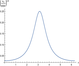
Figure 1: The plot for $\left(\frac{\kappa_{G}}{DDD}\right)^{0.25}$ for torus given by Eq.(4)

The above plot shows that $\left(\frac{\kappa_{G}}{DDD}\right)^{0.25}$ always remains positive irrespective of the sign or value of $\kappa_{G}$ of a surface. The charge density on the torus [11] is a more complicated function of $v$ and is different from the variation shown in figure 1. Thus, the Compensating Factor (CF) that must be multiplied to $\left(\frac{\kappa_{G}}{DDD}\right)^{0.25}$ to obtain the charge density, arises due to the integral factor $\int_{\infty}^{\bf{r_{0}}}$. The value of this factor can be back-calculated if the charge density is already known, using $\left(\frac{\kappa_{G}}{DDD}\right)^{0.25}$. In the following table 1, the summary of all the relevant factors is presented for a few conducting surfaces.

Table 1: Analysis of charge density dependence on various factors

Surface	Parametrization	DDD	$\left(\frac{\kappa}{DDD}\right)^{0.25}$	CF
ellipsoid $\frac{x^{2}}{a^{2}}+\frac{y^{2}}{b^{2}}+\frac{z^{2}}{c^{2}}=1$	$x=a\cos u\sin v$ $y=b\sin u\sin v$ $z=c\cos v$	$\propto\frac{1}{\sin^{4}v}$	$\frac{\kappa^{0.25}}{\sin v}$	$\sin v$
hyperboloid of 2 sheets $\frac{x^{2}}{a^{2}}+\frac{y^{2}}{b^{2}}-\frac{z^{2}}{c^{2}}=-1$	$x=a\sinh u\cos v$ $y=b\sinh u\sin v$ $z=c\cosh u$	$\propto\frac{1}{\sinh^{4}u}$	$\frac{\kappa^{0.25}}{\sinh u}$	$\sinh u$
elliptic paraboloid $\frac{x^{2}}{a^{2}}+\frac{y^{2}}{b^{2}}=z$	$x=a\sqrt{u}\cos v$ $y=b\sqrt{u}\sin v$ $z=u$	constant	$\kappa^{0.25}$	none

5 Application to a boundary value problem

After the discussion in the preceding section and from Eq. (15), it is evident that if in a given boundary value problem, the point ${\bf r_{1}}$ where potential $\Phi=0$ is given, then the charge density will be proportional to:

$$\frac{\Phi_{0}}{\delta A({\bf{r_{o}}})\int_{\bf{r_{1}}}^{\bf{r_{o}}}\left[\frac{{\bf{n}}\cdot{d{\bf{r}}}}{\delta A({\bf{r}})}\right]}$$ (25)

Eq. (25) is the same as Eq. (18) except for the lower limit of the integral of $\left[\frac{{\bf{n}}\cdot{d{\bf{r}}}}{\delta A({\bf{r}})}\right]$. Next, we shall apply Eq. (25) to a boundary value problem and validate the power of this formulation.

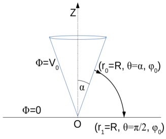
Figure 2: Conducting cone just above a grounded conducting plane

We take a classic example of an infinite conducting cone at potential $V_{0}$ with its apex facing down on a grounded conducting plane [19]. The cone has half-angle $\alpha$ and is open upwards (see figure 2). The apex of the cone is separated from the conducting plane by a tiny air gap (to provide insulation). We try to find the functional form of the charge density on the cone.

The standard method of solving this boundary value problem is to solve the zenith angle dependent part of the Laplace’s equation. This gives the electrostatic potential as a function of $\theta$, i.e. $\Phi=\Phi(\theta)$. The electric field is the negative gradient of this potential. The value of the field close to the given conical conducting surface is proportional to the desired charge density.

However, our formulation directly gives the functional dependence of the electric field, near the conical surface. In this case, the equipotentials are all conical surfaces within the region $\alpha<\theta<\frac{\pi}{2}$. As $\kappa_{G}=0$ on the conical surface, we calculate $\delta A({\bf r_{0}})$ from Eq. (19). The conical surface is parametrized as:

$$x =\frac{r}{a}\cos\phi$$

$$y =\frac{r}{a}\sin\phi$$

$$z =r$$ (26)

Then, we can easily show that $\sqrt{EG-F^{2}}\propto r$. So, at a point ${\bf r_{0}}[=(R,\alpha,\phi_{0})]$ on the surface of the cone, we have:

$$\delta A({\bf r_{0}}) \propto R\ dr\ R\sin\alpha d\phi$$

$$=R^{2}\sin\alpha drd\phi$$ (27)

If we follow a field line that originates from a patch around ${\bf r_{0}}$ on the given conducting conical surface, we see that it reaches the grounded conducting plane at a point ${\bf r_{1}}[=(R,\theta=\frac{\pi}{2},\phi_{0})]$. We notice that only a single variable ($\theta$) varies in this problem. Now, the integral can be evaluated as:

$$\int_{\bf{r_{1}}}^{\bf{r_{o}}}\left[\frac{{\bf{n}}\cdot{d{\bf{r}}}}{\delta A({\bf{r}})}\right] =\int_{\bf{r_{1}}}^{\bf{r_{o}}}\left[\frac{R\ d\theta}{R^{2}\sin\theta\ dr\ d\phi}\right]$$

$$=\frac{1}{R\ dr\ d\phi}\int_{\theta=\frac{\pi}{2}}^{\theta=\alpha}\frac{d\theta}{\sin\theta}$$

$$=\frac{1}{R\ dr\ d\phi}\tan\frac{\alpha}{2}$$ (28)

Therefore, from Eq. (25), Eq. (5) and Eq. (5), the charge density on the conical surface is proportional to:

$$\sigma({\bf r_{0}})\propto\frac{V_{0}}{R\sin\alpha\ \rm{ln}(\tan\frac{\alpha}{2})}$$ (29)

Similarly, one can also derive the charge density on the grounded conducting plane and its value is found to be proportional to $\frac{V_{0}}{R\ \rm{ln}(\tan\frac{\alpha}{2})}$ at a distance $R$ from the origin $O$. It is also possible to directly calculate the electric field in the region $\alpha<\theta<\frac{\pi}{2}$ using Eq. (16). As stated earlier, this formulation is more direct in calculating charge density, compared to the conventional methods.

6 Discussions

In this paper, we reviewed the literature on charge density dependence on conductor surface curvature and tried to establish that these works, though very different in their approaches, are actually related to each other. A number of authors indicated the weak points in these works but the literature were overall silent about how to generalise these results. The connection between the work of Luo [7] and Liu [8] was also not well understood. A recent pedagogical article [15] also could not throw light on this topic.

In this paper, we clarified that the charge density partially depends on $0.25^{th}$ power of the Gaussian curvature of the given conducting surface (through Eq.(21)), though the mean curvature $\kappa_{M}$ of the equipotentials appears in the integral (from ${\bf{r_{0}}}$ to ${\bf{r}}$) in the expression of electric field near the conducting surface in Eq.(14). It is an important point, because the $\kappa_{G}$ is an intrinsic property of a surface whereas $\kappa_{M}$ is not. However, our work indicates that charge density also depends on other functions dependent on surface coordinates. Thus, the dependence on $\kappa_{G}$ cannot be used always to know the distribution of charge on a given conducting surface. In some cases like elliptic paraboloid, it may happen that the contributions from DDD and CF are constants and $\sigma\propto\kappa_{G}^{0.25}$ - but that does not happen in general.

We have shown that when the reference point of the potential is at a finite distance, the integral $\int_{\bf{r_{1}}}^{\bf{r_{0}}}\frac{{\bf n\cdot}d{\bf r}}{\delta A({\bf r})}$ can be evaluated if certain symmetries permit. In this case, the formulation offers a direct way to find the functional dependence of the density of charge. However, if the symmetries do not permit, evaluation of the integral $\int_{\bf r_{1}}^{\bf r_{0}}$ (or $\int_{\infty}^{\bf{r_{0}}}$) seems to be an impossible task, even when the potential depends on a single variable, because the area element $\delta A({\bf r})$, ${\bf n}({\bf r})$ and $d{\bf r}$ gradually evolve along with the different equipotentials. The contribution of this factor into the charge density is quantified by the compensating factor CF. For the examples in table 1, it appears that CF somehow depends on $\frac{dz}{d\xi}$, where $z$ is a function of $\xi$ (in the parametric equation of the surface). But this empirical observation should not be interpreted as a general rule.

7 Acknowledgements

I feel indebted to Dr. Debapriyo Syam for precious encouragements from him while trying to solve the problem. The supports from from my friends Tanmay, Manoneeta and Tamali were also of great help.

References

- [1] David Jeffrey Griffiths and Reed College. Introduction to electrodynamics, volume 3. prentice Hall Upper Saddle River, NJ, 1999.
- [2] Walter Greiner. Classical electrodynamics. Springer Science & Business Media, 2012.
- [3] George Green. An essay on the application of mathematical analysis to the theories of electricity and magnetism, volume 3. author, 1889.
- [4] Ezzat G Bakhoum. Proof of thomson’s theorem of electrostatics. Journal of Electrostatics, 66(11):561–563, 2008.
- [5] GA Estevez and LB Bhuiyan. Power series expansion solution to a classical problem in electrostatics. American Journal of Physics, 53(2):133–134, 1985.
- [6] Richard C Pappas. Differential-geometric solution of a problem in electrostatics. SIAM Review, 28(2):225–227, 1986.
- [7] Luo Enze. The distribution function of surface charge density with respect to surface curvature. Journal of Physics D: Applied Physics, 19(1):1–6, 1986.
- [8] Kun-Mu Liu. Relation between charge density and curvature of surface of charged conductor. American Journal of Physics, 55(9):849–852, 1987.
- [9] IW McAllister. Conductor curvature and surface charge density. Journal of physics. D, Applied physics, 23(3):359–362, 1990.
- [10] Myriam Dubé, Mario Morel, N Gauthier, and AJ Barrett. Comment on“relation between charge density and curvature of surface of charged conductor,”by kun-mu liu [am. j. phys. 55, 849-852 (1987)]. American Journal of Physics, 57:1047–1048, 1989.
- [11] M Torres, JM González, and G Pastor. Comment on“relation between charge density and curvature of surface of charged conductor,”by kun-mu liu [am. j. phys. 55, 849-852 (1987)]. American Journal of Physics, 57:1044–1046, 1989.
- [12] Yuan Zhong Zhang. A comment on’the distribution function of surface charge density with respect to surface curvature’. Journal of Physics D: Applied Physics, 21(7):1235, 1988.
- [13] Luo Enze. The application of a surface charge density distribution function to the solution of boundary value problems. Journal of Physics D: Applied Physics, 20(1):1609–1615, 1987.
- [14] William Ralph Smythe and William R Smythe. Static and dynamic electricity, volume 3. McGraw-Hill New York, 1950.
- [15] Mehdi Jafari Matehkolaee and Ali Naderi Asrami. The review on the charge distribution on the conductor surface. European J Of Physics Education, 4(3), 2013.
- [16] Theodore Frankel. The geometry of physics: an introduction. Cambridge University Press, 2011.
- [17] Shlomo Sternberg. Curvature in mathematics and physics. Courier Corporation, 2012.
- [18] Wolfram Mathematica. Wolfram research. Inc., Champaign, Illinois, 2012.
- [19] Matthew NO Sadiku. Elements of electromagnetics. Oxford university press, 2007.