A method for Hamiltonian truncation: A four-wave example

A method for extracting finite-dimensional Hamiltonian systems from a class of $2+1$ Hamiltonian mean field theories is presented. These theories possess noncanonical Poisson brackets, which normally resist Hamiltonian truncation, but a process of beatification by coordinate transformation near a reference state is described in order to perturbatively overcome this difficulty. Two examples of four-wave truncation of Euler’s equation for scalar vortex dynamics are given and compared: one a direct non-Hamiltonian truncation of the equations of motion, the other obtained by beatifying the Poisson bracket and then truncating.

1 Introduction

The reduction of partial differential equations describing physical phenomena, infinite-dimensional dynamical systems, to ordinary differential equations, finite-dimensional dynamical systems, is a mainstay procedure of physics. This is done on the one hand in order to obtain semi-discrete schemes for numerical computation and on the other to obtain reduced low-dimensional nonlinear models for describing specific physical mechanisms. Examples of the former include finite difference methods such as the Arakawa Jacobian scheme (e.g. Refs.  1; 2) and generalizations (e.g. Ref.  3) or the discontinuous Galerkin method (e.g. Refs.  4; 5), while examples of the latter are low-order modal models. The focus of the present paper is to describe a method for obtaining weakly nonlinear Hamiltonian models from noncanonical Hamiltonian systems,^{6; 7} models that can then be truncated to obtain finite-dimensional Hamiltonian systems. The method is described in general terms and demonstrated explicitly by extracting a four-wave model from Euler’s equation for vorticity dynamics in two dimensions as an example.

Although a plethora of low-order models have been obtained by various means, the three-wave model is an exact highly studied case that can be extracted from physical systems that describe, e.g., fluids, plasmas, and optics (e.g. Refs.  8; 9; 10). Similarly, four-wave models have been widely derived and studied (e.g. Refs.  11; 12; 13; 14; 15; 16; 17). These reductions are obtained from a parent model, a nonlinear partial differential equation, by linearizing about an equilibrium state and analyzing the dispersion relation for the possibilities of three or four-wave resonances between linear eigenmodes. If such exist, these models can be derived by averaging or other means.

Of particular current interest are low-order models for describing the dynamics of zonal flows that occur in geophysical fluid dynamics and plasma physics, in the contexts of planetary atmospheres and the edge tokamaks, respectively. These separate fields of research have common physics as captured by the Charney-Hasegawa-Mima (or quasigeostrophic) equation,^{18; 19} which describes both Rossby waves and plasma drift waves (e.g. Ref.  20). In order to describe effects in tokamaks such as the transition to turbulence due to gradients, the emergence of zonal flows, and barriers to transport, four-wave^{21; 22} and higher dimensional models ^{23; 24} have been proposed, but the Hamiltonian form has either not been determined or has not been obtained from a parent model. The methods of this paper provide a means for doing this.

In general, when dissipative effects are ignored, one may expect systems to possess Hamiltonian structure. This is the case for the three-wave model and is indeed overwhelming the case for systems that describe fluids, plasmas, and other kinds of matter.⁷ The Hamiltonian structure provides access to the great body of lore about such systems; e.g., it is known at the outset that only certain dispersion relations and bifurcations are possible, the structure provides a means for determining nonlinear stability, and because of the well-known theorem of Liouville on the incompressibility of phase space, attractors are not possible (see e.g.  Refs.  25; 26 for examples).

For the three-wave model, the Hamiltonian form was identified after its derivation; however, this form can be obtained directly from the noncanonical Hamiltonian structure, i.e., one in terms of a Poisson bracket in noncanonical variables (see Ref.  7) of the parent model (e.g. Refs.  27; 28), in which case it is seen that the Manley-Rowe relations and other invariants are directly obtained from the Hamiltonian. Similarly, for the four-wave model that describes modulational instability of surface water waves, the Hamiltonian structure can be obtained from a Lagrangian, or equivalently canonical Hamiltonian, description of a parent model (e.g. Ref.  29). We mention that sometimes Hamiltonian four-wave models are proposed a priori³⁰ and then the tools of Hamiltonian dynamics are exploited.

Hamiltonian reduction of the noncanonical Poisson brackets considered here, by means of direct projection onto bases such as Fourier series, is in general not possible because truncation destroys the Jacobi identity.³¹ In the case of two dimensions, the procedure of Refs.  27; 28 that addressed a beam plasma system with one dimension is not workable. This is because the two-dimensional Poisson bracket that describes, e.g., the Charney-Hasegawa-Mima equation and Vlasov-Poisson system (see section 2) depends on the dynamical variable,^{6; 32} and this is the source of difficulty.

In previous work³³ this difficulty was surmounted by a process called beatification, whereby the dynamical variable is removed from the noncanonical Poisson bracket to lowest order by a perturbative transformation about an equilibrium state. In removing the dynamical variable from the Poisson bracket, beatification is a step toward canonization, i.e., transforming to variables in which the Poisson bracket has standard canonical form. The beatification procedure, in eliminating variable dependence from the Poisson bracket, increases the degree of nonlinearity of the Hamiltonian. Then, the Poisson bracket and Hamiltonian can be expanded in a basis and then truncated with the Hamiltonian form being preserved. The present paper builds on previous work³³ by generalizing to expansion about an arbitrary reference state and by continuing the expansion to one higher order. Our example, which as noted above starts from Euler’s equation, is similar but not equivalent to the four-wave model of Refs.  21; 22, since the latter starts from the modified Hasegawa-Mima equation.

We note that there is literature on the general problem of extracting reduced noncanonical Hamiltonian systems from a parent Hamiltonian system by expansion in a small parameter. A procedure was introduced in Refs.  34; 35 with water waves as an application, described as a general deformation of Poisson brackets on Poisson manifolds in Ref.  36, and placed in the context of generalized Lie transforms in Ref.  37. Central to all these developments is the Schouten bracktet³⁸. These works concern expansion about a dynamical system in order to produce a new, possibly noncanonical, Hamiltonian dynamical system, while beatification is an expansion about a phase space point that produces a constant Poisson bracket.

The paper is organized as follows. In section 2, we introduce a general class of Hamiltonian systems that share a common noncanonical Poisson bracket and associated Casimir invariants, constants of motion associated with the bracket degeneracy. Depending on the choice of Hamiltonian, this class includes the Hamiltonian descriptions of the Vlasov-Poisson system, quasigeostrophy and other mean field theories, but of main concern is the example we treat, the two-dimensional Euler system for the dynamics of the scalar vorticity. In section 3 we perform a direct truncation. To this end the noncanonical Poisson bracket is transformed in subsection 3.1 by considering dynamics relative to an arbitrary given reference state. The reference state for our four-wave example is introduced here. Then in subsection 3.2 the transformed Poisson bracket is re-expressed by expanding the new dynamical variable in terms of a Fourier series. With any Hamiltonian written in terms of the Fourier series, an infinite-dimensional dynamical system is obtained for the Fourier amplitudes. This is worked out for the Euler example. A truncation is done in subsection 3.3, producing a four-wave system, which is seen in subsection 3.4 to conserve a reduced form of the energy and to possess a remnant of a Casimir invariant of the unreduced system. However, this system is shown in subsection 3.5 not to be Hamiltonian because the truncated bracket does not satisfy the Jacobi identity. In section 4 we describe beatification, the procedure by which variable dependence is removed from the noncanonical Poisson bracket, and then we apply it to the bracket presented in section 2. Fourier expansion of the beatified Poisson bracket is done in subsection 5.1 which prepares the way for Hamiltonian truncation. Although one can truncate by retaining any number of Fourier amplitudes, we demonstrate the method for our four-wave example in subsection 5.2. Contrary to subsection 3.4, it is observed in subsection 5.3 that two Casimir invariants are obtained for our four-wave Hamiltonian example. In section 6 we use the notion of a recurrence plot to give some preliminary numerical evidence for the superiority of the Hamiltonian truncation of subsection 5.2. Finally, in section 7, we summarize the main findings of our work and make some concluding remarks.

2 A class of Hamiltonian systems

We begin by describing a general class of Hamiltonian systems, 2+1 mean field theories. First we give the Hamiltonian then describe the Poisson bracket and associated Casimir invariants.

We take as a basic dynamical variable a scalar density or vorticity-like quantity, $\omega(r,t)$, which is a real-valued function defined on a two-dimensional domain $\mathcal{D}$. For the present development we assume Cartesian coordinates where $r=(x,y)\in\mathcal{D}$. A general class of Hamiltonian mean field theories³⁹ possess a Hamiltonian (energy) functional contained in the following form:

$$H[\omega]=\int_{\mathcal{D}}\mathrm{d}^{2}r\;\omega(r,t)\,h_{1}(r)+\frac{1}{2}\int_{\mathcal{D}}\mathrm{d}^{2}r\!\int_{\mathcal{D}}\mathrm{d}^{2}r^{\prime}\;\omega(r,t)\,h_{2}(r;r^{\prime})\,\omega(r^{\prime},t)\,,$$ (1)

where $\mathrm{d}^{2}r=\mathrm{d}x\mathrm{d}y$. The first term of (1), the inertial term, represents energy associated with free motion as determined by the function $h_{1}$, while the second term, the interaction term, represents the energy of two-point interaction as determined by the function $h_{2}$. One could generalize this with three-point and higher interactions in an obvious way.

Hamiltonians of the form of (1) include the examples below for well-known systems:

• when $\omega$ is the phase space density for a species of mass $m$ and charge $e$, $\mathcal{D}=\mathbb{R}^{2}$ the phase space for a one degree-of-freedom system, for which $r=(x,v)\in\mathcal{D}$ with velocity $v$, kinetic energy $h_{1}=mv^{2}/2$, and interaction potential $h_{2}=e|x-x^{\prime}|$ for charged sheets, (1) is the energy for the Vlasov-Poisson system.⁴⁰

• when $\omega$ is the scalar vorticity, then $\mathcal{D}$ denotes the planar domain occupied by the fluid. Upon choosing $h_{1}\equiv 0$ and defining $\Delta^{-1}$ to be the formal inverse of the two-dimensional Laplacian operator $\Delta=\partial_{x}^{2}+\partial_{y}^{2}$, then (1) is the Hamiltonian for Euler’s equation describing an ideal, incompressible and two-dimensional fluid^{32; 7}

  $$H[\omega]=-\frac{1}{2}\int_{\mathcal{D}}\mathrm{d}^{2}r\;\omega\Delta^{-1}\omega\,.$$ (2)

  For this case $h_{2}$ is proportional to the Green’s function corresponding with $\Delta$. This case will be the starting point for the four-wave example treated in our paper.

• when $\omega$ is the charge density for drift waves or the potential vorticity of geophysical fluid dynamics, then $\omega=b(x)-\mathcal{L}\psi$, where for the Hasegawa-Mima equation or quasigeostrophy $\mathcal{L}:=\Delta+\kappa^{2}$, $\psi$ is the electrostatic potential or stream function, and $b$ represents the electron density or $\beta$-effect, respectively, with $\kappa^{-1}$ measuring the Rossby deformation radius. For this case the Hamiltonian is⁴¹

  $$H[\omega]=\int_{\mathcal{D}}\mathrm{d}^{2}r\left(\omega\,\mathcal{L}^{-1}b-\frac{1}{2}\,\omega\mathcal{L}^{-1}\omega\right)\,.$$ (3)

  Note, $\mathcal{L}$ could be any invertible elliptic operator.

To define the Poisson bracket we require the functional derivative, which is defined as usual by

$$\delta H[\omega;\delta\omega]=\left.\frac{d}{d\epsilon}H[\omega+\epsilon\delta\omega]\right|_{\epsilon=0}=\int_{\mathcal{D}}\mathrm{d}^{2}r\,\delta\omega\frac{\delta H}{\delta\omega}\,,$$ (4)

where $\delta\omega(r,t)$ is a variation of $\omega$. (See e.g. Ref. [ 7] for details.) For the Hamiltonian of (1) we have

$$\frac{\delta H}{\delta\omega}=h_{1}+\int_{\mathcal{D}}\mathrm{d}^{2}r^{\prime}\;h_{2}(r;r^{\prime})\,\omega(r^{\prime},t)\,,$$ (5)

a quantity that will be inserted into a Poisson bracket. The Poisson bracket for our class of theories is given by the following bilinear product between two arbitrary functionals of the field $\omega$:

$$\{F,G\}=\int_{\mathcal{D}}\mathrm{d}^{2}r\;\omega\left[\frac{\delta F}{\delta\omega},\frac{\delta G}{\delta\omega}\right]=\int_{\mathcal{D}}\mathrm{d}^{2}r\;\frac{\delta F}{\delta\omega}\mathcal{J}(\omega)\frac{\delta G}{\delta\omega}\,,$$ (6)

where $[f,g]=(\partial_{x}f)(\partial_{y}g)-(\partial_{y}f)(\partial_{x}g)$, with $f$ and $g$ being two arbitrary functions on the domain $\mathcal{D}$. Proofs of the Jacobi identity for (6) were given by direct computation in Ref.  31 and by Clebsch reduction in Ref.  32. We note, it can also be shown by the vanishing of the Schouten bracket (e.g. Ref.  34). Comparison of the two integrals of (6) gives the Poisson operator

$$\mathcal{J}(\omega)f=-\left[\omega,f\right]\,,$$ (7)

in which $f$ is again an arbitrary function. Notice that the two integrals shown in equation (6) may differ by a boundary term that could be associated with boundary contour dynamics. Here we consider periodic boundary conditions, $\mathcal{D}$ is a two-torus, and consequently boundary terms are readily eliminated upon integrations by parts. Thus, $\mathcal{D}$ is a rectangular domain with edges aligned along Cartesian axes and normalized to unity so $x,y\in[0,1)$.

The equation of motion for $\omega$ follows from the Poisson bracket according to

$$\frac{\partial\omega}{\partial t} =\{\omega,H\}=\mathcal{J}(\omega)\frac{\delta H}{\delta\omega}$$ (8)

$$=-\left[\omega,h_{1}+\int_{\mathcal{D}}\mathrm{d}^{2}r^{\prime}\;h_{2}\,\omega\right]\,,$$

where the second line follows upon insertion of (5). For Euler’s Hamiltonian of equation (2), $h_{1}=0$ and $h_{2}=-\delta(r-r^{\prime})\Delta^{-1}$.

Noncanonical Poisson brackets like (6) are degenerate and this gives rise to the so-called Casimir invariants. An easy calculation shows that

$$\mathcal{C}[\omega]=\int_{\mathcal{D}}\mathrm{d}^{2}r\,f(\omega)\,,$$ (9)

where $f$ is an arbitrary function of $\omega$, is a constant of motion for any Hamiltonian. Such quantities, Casimir invariants, satisfy

$$\{F,\mathcal{C}\}=0$$ (10)

for any functional $F[\omega]$. In older plasma literature Casimir invariants were called generalized entropies. For convenience, the following family of Casimirs is often used:

$$\mathcal{C}^{(n)}[\omega]=\int_{\mathcal{D}}\,\omega^{n}\,\mathrm{d}^{2}r,$$ (11)

for $n\in\mathbb{N}$. For vortex dynamics the case $n=1$ corresponds to the total vorticity, while $n=2$ is generally called the enstrophy.

3 Direct truncation

Equation (8) is an infinite-dimensional Hamiltonian system for the field $\omega$. Our goal is to extract from it a finite-dimensional Hamiltonian system. We proceed by expressing (8) in a Fourier series, which we then truncate to obtain a four-wave model. This is done in two parts, first for the Poisson bracket, then for the specific Hamiltonian of Euler’s equation; however, the procedure could be carried out for any Hamiltonian. We will see that this approach leads to a system that is energy conserving, but it does not lead to Hamiltonian form. Our approach can be viewed as an attempt to obtain a Hamiltonian truncation by following the prescription of Refs.  21; 22 for Euler’s equation, although in a more general setting. This section is broken up into several subsections that contain calculations of relevance to sections 4 and 5, where we make comparison with a truncated system obtained by our beatification procedure.

3.1 Reference state

The first step of our calculation is to consider dynamics relative to an arbitrary reference state,

$$\omega(x,y;t)=\omega_{0}(x,y)+\varepsilon\mu(x,y;t),$$ (12)

where $\omega_{0}$ is the reference state, a chosen time-independent function, $\mu$ is a new dynamical field, and $\varepsilon$ is a perturbative bookkeeping parameter. For situations where the field $\mu$ describes a small deviation from $\omega_{0}$, which will occur for sufficiently short time intervals, we can expand using $\varepsilon\ll 1$ to obtain reduced models.

As a preparatory step for the decomposition of the quantities (2) and (6) into the vorticity Fourier amplitudes, we transform the Poisson bracket from one in terms of the field $\omega$ to one in terms of $\mu$. A straightforward functional chain rule calculation (see Ref.  7) gives

$$\{F,G\}=\frac{1}{\varepsilon^{2}}\int_{\mathcal{D}}\mathrm{d}^{2}r\,\frac{\delta F}{\delta\mu}\mathcal{J}_{\varepsilon}(\mu)\frac{\delta G}{\delta\mu},$$ (13)

where $\mathcal{J}_{\varepsilon}(\mu)=\mathcal{J}(\omega_{0}+\varepsilon\mu)$ is the new Poisson operator.

Next, inserting (12) into the Hamiltonian of (2) gives

$$H[\mu]=-\frac{1}{2}\int_{\mathcal{D}}\mathrm{d}^{2}r\,\left(\omega_{0}\Delta^{-1}\omega_{0}+2\varepsilon\mu\Delta^{-1}\omega_{0}+\varepsilon^{2}\mu\Delta^{-1}\mu\right).$$ (14)

The Hamiltonian of (14) together with the Poisson bracket of (13) generates the exact Euler’s equation. For this case we expand and project to reduce the dynamics.

In principle, we need not select a specific form for the reference state $\omega_{0}$ in the construction of most of our future results. However, when the Hamiltonian and Poisson bracket are projected onto Fourier modes, the following particular form of the function $\omega_{0}$ is chosen for our four-wave model:

$$\omega_{0}=\omega_{\alpha}\mathrm{e}^{2\pi\mathrm{i}\alpha x}+\omega_{\alpha}^{*}\mathrm{e}^{-2\pi\mathrm{i}\alpha x}+\omega_{\beta}\mathrm{e}^{2\pi\mathrm{i}\beta y}+\omega_{\beta}^{*}\mathrm{e}^{-2\pi\mathrm{i}\beta y}\,,$$ (15)

where $\omega_{\alpha}$ and $\omega_{\beta}$ are constant complex amplitudes for modes aligned with the $x$ and $y$ axes, respectively. The quantities $2\pi\alpha$ and $2\pi\beta$, for $\alpha,\beta\in\mathbb{Z}\setminus\!\{0\}$, are wave numbers for the two independent Fourier modes considered; thus, (15) is the superposition of two real orthogonal waves with fixed wavelengths and zero frequency. This reference state is the simplest configuration that, as shown in section 5, allows the construction of a Hamiltonian model with four mutually interacting waves.

3.2 Fourier decomposition

We perform a Fourier decomposition within the Hamiltonian description, i.e., both the Poisson bracket (13) and our example with the Hamiltonian of (2) for vorticity dynamics are written in terms of Fourier series, giving a countably infinite-dimensional Hamiltonian system. We expand

$$\mu(x,y;t)=\sum\limits_{j,k=-\infty}^{\infty}\mu_{j,k}(t)\mathrm{e}^{2\pi\mathrm{i}(jx+ky)},$$ (16)

where the amplitudes $\mu_{j,k}$ are time dependent and, because $\mu$ is a real-valued field, satisfy the reality condition $\mu_{j,k}^{*}=\mu_{-j,-k}$.

Substitution of (16) into an arbitrary functional $F[\mu]$ and calculation of the spatial integrals yields a function of all of the Fourier amplitudes, which we will denote by $\bar{F}(\mu_{j,k})$. Thus, under this variable change $F[\mu]=\bar{F}(\mu_{j,k})$. As can be readily shown (see Ref.  7), the derivatives of the function $\bar{F}$ are related to the functional derivative of $F$ by the following identity:

$$\frac{\partial\bar{F}}{\partial\mu^{*}_{j,k}}=\left(\frac{\delta F}{\delta\mu}\right)_{j,k}\,.$$ (17)

Since $\delta F/\delta\mu$ is a function of $x$ and $y$ it can also be Fourier expanded,

$$\frac{\delta F}{\delta\mu}=\sum\limits_{j,k=-\infty}^{\infty}\left(\frac{\delta F}{\delta\mu}\right)_{j,k}\mathrm{e}^{2\pi\mathrm{i}(jx+ky)}.$$ (18)

Then, substitution of (15), (16), (17), and (18) into (13), gives the Poisson bracket in terms of the dynamical variables $\mu_{j,k}$,

$$\{\bar{F},\bar{G}\}= -\left(\frac{2\pi}{\varepsilon}\right)^{2}\sum\limits_{j,k=-\infty}^{\infty}\frac{\partial\bar{F}}{\partial\mu_{j,k}^{*}}\left[\alpha k\omega_{\alpha}\frac{\partial\bar{G}}{\partial\mu_{(j+\alpha),k}}-\alpha k\omega_{\alpha}^{*}\frac{\partial\bar{G}}{\partial\mu_{(j-\alpha),k}}-j\beta\omega_{\beta}\frac{\partial\bar{G}}{\partial\mu_{j,(k+\beta)}}\right.$$ (19)

$$\left.+j\beta\omega_{\beta}^{*}\frac{\partial\bar{G}}{\partial\mu_{j,(k-\beta)}}+\varepsilon\sum\limits_{m,n=-\infty}^{\infty}(km-jn)\mu_{m,n}\frac{\partial\bar{G}}{\partial\mu_{(j+m),(k+n)}}\right].$$

Any Hamiltonian functional of the form of (1) can be projected, $H[\mu]=\bar{H}(\mu_{j,k})$, but for simplicity we will only consider the special case of (14) corresponding to Euler’s equation. Accordingly, inserting (15) and (16) into (14), yields the following Hamiltonian function:

$$\bar{H}= \frac{1}{4\pi^{2}}\left[\frac{1}{\alpha^{2}}\left(\omega_{\alpha}^{*}\omega_{\alpha}+\varepsilon\omega_{\alpha}\mu_{\alpha,0}^{*}+\varepsilon\omega_{\alpha}^{*}\mu_{\alpha,0}\right)+\frac{1}{\beta^{2}}\left(\omega_{\beta}^{*}\omega_{\beta}+\varepsilon\omega_{\beta}\mu_{0,\beta}^{*}+\varepsilon\omega_{\beta}^{*}\mu_{0,\beta}\right)\right]$$ (20)

$$+\frac{\varepsilon^{2}}{8\pi^{2}}\sum\limits_{j,k=-\infty}^{\infty}\frac{\mu_{j,k}^{*}\mu_{j,k}}{j^{2}+k^{2}}\,,$$

where in deriving (20) we have used the identity $f_{j,k}=-\frac{1}{(2\pi)^{2}}\frac{g_{j,k}}{j^{2}+k^{2}}$ which follows from $f=\Delta^{-1}g$.

Finally, with the Hamiltonian of (20) and the bracket of (19), the equations of motion for the Fourier amplitudes of the perturbative field are given in the following Hamiltonian form:

$$\dot{\mu}_{j,k} =\{\mu_{j,k},\bar{H}\}$$ (21)

$$=\frac{1}{\varepsilon}\sum\limits_{m,n=-\infty}^{\infty}\frac{jn-km}{m^{2}+n^{2}}\big{(}\omega_{m,n}+\varepsilon\mu_{m,n}\big{)}\,\big{(}\omega_{j-m,k-n}+\varepsilon\mu_{j-m,k-n}\big{)},$$

where, in order to simplify this expression, we introduced the definition

$$\omega_{m,n}=\omega_{\alpha}\delta_{m,\alpha}\delta_{n,0}+\omega_{\alpha}^{*}\delta_{m,-\alpha}\delta_{n,0}+\omega_{\beta}\delta_{m,0}\delta_{n,\beta}+\omega_{\beta}^{*}\delta_{m,0}\delta_{n,-\beta}\,.$$ (22)

3.3 A four-wave truncation

So far, no approximations have been made, only a shift of the dependent variable and Fourier expansion. Now we truncate (21), with the objective of highlighting the major disturbances on the reference state for sufficiently short periods of time. For this reason, an adequate implementation of the truncation process must preserve the Fourier coefficients of $\mu$ representing direct changes of amplitudes with the same wave numbers as those of the reference state of (15). Thus, we retain the amplitudes corresponding to the following wave vectors:

$$\vec{k}_{\alpha,0}=2\pi(\begin{array}[]{c c}\alpha&0\end{array})^{T},$$ (23b)

$$\vec{k}_{0,\beta}=2\pi(\begin{array}[]{c c}0&\beta\end{array})^{T},$$ (23d)

$$\vec{k}_{-\alpha,0}=2\pi(\begin{array}[]{c c}-\alpha&0\end{array})^{T}=-\vec{k}_{\alpha,0},$$ (23f)

$$\vec{k}_{0,-\beta}=2\pi(\begin{array}[]{c c}0&-\beta\end{array})^{T}=-\vec{k}_{0,\beta}\,,$$ (23h)

where $T$ denotes transpose. Notice that the Fourier amplitudes labeled by the wave vectors $\vec{k}_{-\alpha,0}$ and $\vec{k}_{0,-\beta}$ are not independent of those labeled by $\vec{k}_{\alpha,0}$ and $\vec{k}_{0,\beta}$ because of the reality conditions on $\omega_{0}$ and $\mu$.

As seen from (21), the value of $\dot{\mu}_{j,k}$ results from a summation over specific quadratic terms, products of Fourier amplitudes with corresponding wave vectors summing to $\vec{k}_{j,k}=2\pi(\begin{array}[]{c c}j&k\end{array})^{T}$. Therefore, given that the modes associated with the wave vectors (23) are the only ones with relevant initial amplitudes in the field $\omega$, then the only amplitudes with significant initial time variation are those associated with the following wave vectors:

$$\vec{k}_{\alpha,\beta}=2\pi(\begin{array}[]{c c}\alpha&\beta\end{array})^{T},$$ (24b)

$$\vec{k}_{\alpha,-\beta}=2\pi(\begin{array}[]{c c}\alpha&-\beta\end{array})^{T},$$ (24d)

$$\vec{k}_{-\alpha,\beta}=2\pi(\begin{array}[]{c c}-\alpha&\beta\end{array})^{T},$$ (24f)

$$\vec{k}_{-\alpha,-\beta}=2\pi(\begin{array}[]{c c}-\alpha&-\beta\end{array})^{T}.$$ (24h)

Recall, the identities $\vec{k}_{\alpha,\beta}=-\vec{k}_{-\alpha,-\beta}$ and $\vec{k}_{\alpha,-\beta}=-\vec{k}_{-\alpha,\beta}$ imply $\mu_{\alpha,\beta}^{*}=\mu_{-\alpha,-\beta}$ and $\mu_{\alpha,-\beta}^{*}=\mu_{-\alpha,\beta}$; that is, the four wave vectors shown in equation (24) correspond to only two independent complex amplitudes.

Also in accordance with (21), note that the amplitudes resulting from the vectors (24) have dominant temporal variations in terms of $\varepsilon$. In other words, the differential equations for the velocities $\dot{\mu}_{\alpha,\beta}$ and $\dot{\mu}_{\alpha,-\beta}$ are the only ones that have leading order terms independent of the perturbative field $\mu$. This property, together with the arguments mentioned in previous paragraphs, justifies the retention of complex amplitudes associated with wave vectors (23) and (24) as dynamical variables in our truncation, specifically considering the reference state (15).

For convenience we define

$$\hat{\mu} =(\mu_{\alpha,0},\,\mu_{0,\beta},\,\mu_{\alpha,\beta},\,\mu_{\alpha,-\beta},\,\mu_{-\alpha,0},\,\mu_{0,-\beta},\,\mu_{-\alpha,-\beta},\,\mu_{-\alpha,\beta})$$ (25)

$$=(\mu_{\alpha,0},\,\mu_{0,\beta},\,\mu_{\alpha,\beta},\,\mu_{\alpha,-\beta},\,\mu_{\alpha,0}^{*},\,\mu_{0,\beta}^{*},\,\mu_{\alpha,\beta}^{*},\,\mu_{\alpha,-\beta}^{*})$$

for the amplitudes that survive the truncation. Observe that $\hat{\mu}$ has eight components, four independent complex variables.

Now consider the Poisson bracket. By retaining modes with the amplitudes of (25) the Poisson bracket of (19) can be truncated to the following bilinear operation between two arbitrary functions on the truncated phase space:

$$\{f,g\}_{\hat{\mu}}=\left(\frac{\partial f}{\partial\hat{\mu}}\right)^{T}\!\!\cdot J_{\hat{\mu}}\cdot\left(\frac{\partial g}{\partial\hat{\mu}}\right),$$ (26)

where $\partial/\partial\hat{\mu}$ symbolizes the eight-dimensional gradient in the coordinates of (25), and the Poisson operator when truncated becomes the following matrix:

$$J_{\hat{\mu}}=-\frac{4\pi^{2}\alpha\beta}{\varepsilon}\left(\begin{array}[]{c c c c c c c c}0&\mu_{\alpha,\beta}&0&0&0&-\mu_{\alpha,-\beta}&-\varpi_{0,\beta}^{*}&\varpi_{0,\beta}\\ -\mu_{\alpha,\beta}&0&0&-\varpi_{\alpha,0}&\mu_{\alpha,-\beta}^{*}&0&\varpi_{\alpha,0}^{*}&0\\ 0&0&0&0&\varpi_{0,\beta}&-\varpi_{\alpha,0}&0&0\\ 0&\varpi_{\alpha,{0}}&0&0&-\varpi_{0,\beta}^{*}&0&0&0\\ 0&-\mu_{\alpha,-\beta}^{*}&-\varpi_{0,\beta}&\varpi_{0,\beta}^{*}&0&\mu_{\alpha,\beta}^{*}&0&0\\ \mu_{\alpha,-\beta}&0&\varpi_{\alpha,0}&0&-\mu_{\alpha,\beta}^{*}&0&0&-\varpi_{\alpha,0}^{*}\\ \varpi_{0,\beta}^{*}&-\varpi_{\alpha,0}^{*}&0&0&0&0&0&0\\ -\varpi_{0,\beta}&0&0&0&0&\varpi_{\alpha,0}^{*}&0&0\end{array}\right),$$ (27)

in which, for convenience, we introduced two new auxiliary quantities $\varpi_{\alpha,0}=\varepsilon^{-1}\omega_{\alpha}+\mu_{\alpha,0}$ and $\varpi_{0,\beta}=\varepsilon^{-1}\omega_{\beta}+\mu_{0,\beta}$.

Next we truncate the Hamiltonian of (20) by retaining only the eight Fourier amplitudes of $\hat{\mu}$, giving

$$\bar{H}_{\hat{\mu}}= \frac{1}{4\pi^{2}}\left[\frac{1}{\alpha^{2}}(\omega_{\alpha}^{*}+\varepsilon\mu_{\alpha,0}^{*})(\omega_{\alpha}+\varepsilon\mu_{\alpha,0})+\frac{1}{\beta^{2}}(\omega_{\beta}^{*}+\varepsilon\mu_{0,\beta}^{*})(\omega_{\beta}+\varepsilon\mu_{0,\beta})\right.$$ (28)

$$\left.+\frac{\varepsilon^{2}}{\alpha^{2}+\beta^{2}}(\mu_{\alpha,\beta}^{*}\mu_{\alpha,\beta}+\mu_{\alpha,-\beta}^{*}\mu_{\alpha,-\beta})\right].$$

Similar expressions can be obtained for the Hamiltonians described in section 2, in particular, for the Hamitlonian of (3) additional terms would be added to (28).

Using the results (26) and (28), the truncated equations of motion take the following form:

$$\dot{\hat{\mu}}=J_{\hat{\mu}}\cdot\frac{\partial\bar{H}_{\hat{\mu}}}{\partial\hat{\mu}}\,,$$ (29)

which gives our four-wave model,

$$\dot{\mu}_{\alpha,0}=\alpha\beta\left(\frac{1}{\beta^{2}}-\frac{1}{\alpha^{2}+\beta^{2}}\right)\left[(\omega_{\beta}+\mu_{0,\beta})\mu_{\alpha,-\beta}-(\omega_{\beta}^{*}+\mu_{0,\beta}^{*})\mu_{\alpha,\beta}\right],$$ (30a)

$$\dot{\mu}_{0,\beta}=\alpha\beta\left(\frac{1}{\alpha^{2}}-\frac{1}{\alpha^{2}+\beta^{2}}\right)\left[(\omega_{\alpha}^{*}+\mu_{\alpha,0}^{*})\mu_{\alpha,\beta}-(\omega_{\alpha}+\mu_{\alpha,0})\mu_{\alpha,-\beta}^{*}\right],$$ (30b)

$$\dot{\mu}_{\alpha,\beta}=\alpha\beta\left(\frac{1}{\beta^{2}}-\frac{1}{\alpha^{2}}\right)(\omega_{\alpha}+\mu_{\alpha,0})(\omega_{\beta}+\mu_{0,\beta}),$$ (30c)

$$\dot{\mu}_{\alpha,-\beta}=\alpha\beta\left(\frac{1}{\alpha^{2}}-\frac{1}{\beta^{2}}\right)(\omega_{\alpha}+\mu_{\alpha,0})(\omega_{\beta}^{*}+\mu_{0,\beta}^{*}),$$ (30d)

where we omit the equations for the complex conjugate amplitudes, since they are apparent, and we set $\varepsilon=1$ because retention of $\varepsilon$ is not necessary, the perturbation order being the same as the polynomial degree of $\hat{\mu}$.

Alternative to the procedure adopted above, we could have obtained the dynamical system of (30) directly by truncating equations (21). However, we chose to truncate the Poisson bracket and the Hamiltonian function, as these results will be important for our discussions in the following sections.

3.4 Constants of motion

Having obtained our equations of motion in the form of (29), the question of which constants of motion survive the truncation arises. Because of the evident antisymmetry of the matrix of (27), it is clear that any (autonomous) Hamiltonian used to generate the dynamics will be conserved. Thus, this is the case for $\bar{H}_{\hat{\mu}}$ of (28). However, clearly not all of the infinite number of Casimirs $\mathcal{C}^{(n)}$ of $\eqref{eq:2.6}$ can survive, because Casimirs are associated with the null space of $J_{\hat{\mu}}$ which must be finite. One can directly calculate the null eigenvectors of the matrix of (27), and then integrate a linear combination of them to obtain the following Casimir invariant:

$$\bar{\mathcal{C}}^{(2)}_{\hat{\mu}}= 2\left[(\omega_{\alpha}^{*}+\mu_{\alpha,0}^{*})(\omega_{\alpha}+\mu_{\alpha,0})+(\omega_{\beta}^{*}+\mu_{0,\beta}^{*})(\omega_{\beta}+\mu_{0,\beta})\right.$$ (31)

$$\left.+\mu_{\alpha,\beta}^{*}\mu_{\alpha,\beta}+\mu_{\alpha,-\beta}^{*}\mu_{\alpha,-\beta}\right].$$

Alternatively, one expects the quadratic Casimir to survive, it being a so-called rugged invariant.⁴² Thus, inserting the transformation (12) into (11) for $n=2$ gives the candidate

$$\mathcal{C}^{(2)}[\mu]=\int_{\mathcal{D}}\mathrm{d}^{2}r\left(\omega_{0}^{2}+2\varepsilon\omega_{0}\mu+\varepsilon^{2}\mu^{2}\right).$$ (32)

Employing the expansion (16) to the above yields

$$\bar{\mathcal{C}}^{(2)}=2(\omega_{\alpha}^{*}\omega_{\alpha}+\omega_{\beta}^{*}\omega_{\beta}+\omega_{\alpha}\mu_{\alpha,0}^{*}+\omega_{\alpha}^{*}\mu_{\alpha,0}+\omega_{\beta}\mu_{0,\beta}^{*}+\omega_{\beta}^{*}\mu_{0,\beta})+\sum\limits_{j,k=-\infty}^{\infty}\mu_{j,k}^{*}\mu_{j,k},$$ (33)

where the parameter $\varepsilon$ was set to unit. Then upon truncating (33), i.e., retaining only the complex amplitudes present in (25), indeed we obtain (31).

3.5 The Jacobi identity

So far, we have performed a truncation of the Hamiltonian formulation for the two-dimensional Euler equation, yielding the four-wave dynamical system of equations (30a)–(30d). En route we obtained the invariant function $\bar{H}_{\hat{\mu}}$ and the bilinear operation of (26). However, the resulting system, although energy conserving, cannot be said to be Hamiltonian unless the $J_{\hat{\mu}}$ of (27) when inserted into (26) produces a bracket that satisfies the Jacobi identity. In the present section we briefly review features of finite-dimensional noncanonical Hamiltonian systems, present the Jacobi identity, and discuss its failure for $J_{\hat{\mu}}$.

In conventional physics texts, Hamiltonian dynamics is presented in terms of canonical coordinates and momenta, for which a coordinate free geometric approach^{43; 44} is available. Alternatively, one can consider a noncanonical Hamiltonian framework based on the Lie algebraic properties of the Poisson bracket (e.g., Refs.  45; 32; 7), where coordinates need not be canonical and degeneracy in the Poisson bracket is allowed. (See, e.g., Ref.  46 for geometrical description.) Such a formulation occurs naturally in a variety of contexts, notably the Eulerian variable description of matter, where many fluid and plasma applications have been treated,^{47; 7; 6; 48; 32} and also in the context of semiclassical approximations with generalized coherent states.^{49; 50}

We consider a space (manifold) with $N$ real coordinates, $z=(z^{1},z^{2},\ldots,z^{N})$, and define a bilinear operation between two arbitrary functions as follows:

$$\{f,g\}=\left(\frac{\partial f}{\partial z}\right)^{T}\!\!\!\cdot J(z)\cdot\frac{\partial g}{\partial z},$$ (34)

where $\partial/\partial z$ represents the gradient in the coordinates $z$ and $J(z)$ in (34) is a matrix with possible functional dependence on $z$.

Thus far no restrictions have been placed on the matrix $J(z)$; however, in order for (34) to be a Poisson bracket, two additional conditions are required. First, it must be antisymmetric

$$\{f,g\}=-\{g,f\}\,,$$ (35)

and second it must satisfy the Jacobi identity,

$$\{f,\{g,h\}\}+\{g,\{h,f\}\}+\{h,\{f,g\}\}=0\,.$$ (36)

Properties (35) and (36) imply conditions on the matrix $J(z)$, viz.

$$J^{ab}=-J^{ba}$$ (37a)

$$J^{ad}\frac{\partial J^{bc}}{\partial z^{d}}+J^{bd}\frac{\partial J^{ca}}{\partial z^{d}}+J^{cd}\frac{\partial J^{ab}}{\partial z^{d}}=0,$$ (37b)

which if true for all $a,b,c=1,2,\ldots,N$ are equivalent to (35) and (36). Note, in (37b) repeated sum notation is assumed. When both of the above conditions are met, we call $J(z)$ a Poisson matrix. Note that (37b) is immediately satisfied by a matrix with no dependence on the variables $z$. That is, a skew-symmetric matrix with constant elements automatically produces a Poisson bracket.

Given a Poisson matrix $J(z)$, the Hamiltonian equations of motion are

$$\dot{z}^{a}=\{z^{a},{H}\}=J^{ab}\frac{\partial{H}}{\partial z^{b}},$$ (38)

for $a,b=1,2,\ldots,N$, where the function ${H}(z)$ is the Hamiltonian.

The definition (38) is a quite general (coordinate dependent) formulation of a Hamiltonian system. In particular, we say that the dynamical system (38) is in canonical form if its Poisson matrix is

$$J_{c}=\left(\begin{array}[]{c c}0_{r\times r}&\mathds{1}_{r\times r}\\ -\mathds{1}_{r\times r}&0_{r\times r}\end{array}\right),$$ (39)

where $0_{r\times r}$ and $\mathds{1}_{r\times r}$ denote, respectively, the zero and identity matrices of order $r=N/2$, canonical systems being even dimensional.

Returning to the case at hand, the matrix of (27), we have demonstrated by inserting this $J_{\hat{\mu}}$ into the left-hand-side of (37b) its failure to vanish. Therefore, (26) is not a Poisson bracket, and the equations of motion (30) are not a Hamiltonian system with (28) as Hamiltonian. This failure of the Jacobi identity is not surprising, since it has been known for some time that direct Fourier truncation destroys the Jacobi identity.³¹

There is a caveat to our result. Strictly speaking, we have not demonstrated the absence of any Hamiltonian formulation for the system (30) – we have only shown that the elements of identity (29) do not define a Hamiltonian system. We cannot exclude the possibility that equations (30) could result from some unknown Poisson matrix together with some invariant Hamiltonian function. However, since the system (30) follows from the truncation of a Hamiltonian model, we believe the existence of a Hamiltonian formulation arising from quantities uncorrelated with the truncated values of the expressions (13) and (14) is unlikely. Moreover, we have not been able to find any additional invariants that might serve as candidate Hamiltonians.

Another feature of the failure of the Jacobi identity is worth mentioning. Because (27) is antisymmetric, its rank must be even, which in our case is six. For Hamiltonian systems, the existence of two null eigenvectors implies the existence of two Casimir invariants; a consequence of the Jacobi identity is that the null space of the Poisson matrix is spanned by gradients of Casimir invariants. However, for the $J_{\hat{\mu}}$ of (27), there is only one independent function whose gradient is a null eigenvector, even though (27) has a two-dimensional null space. This is another manifestation of the fact that the matrix $J_{\hat{\mu}}$ does not satisfy the Jacobi identity.

4 Beatification

Now we perform the beatification procedure,³³ a perturbative transformation that removes the functional dependence of the Poisson operator on the field variable and replaces it with a reference state. The procedure is applied to the bracket of (13) and, in preparation for the truncation procedure of section 5, the Hamiltonian for the two-dimensional Euler equation is expressed in terms of the transformed variable.

The beatification procedure has two parts. The first part involves the Poisson bracket, with the original field shifted by introducing a sum of a reference state and a perturbative field as was done in equation (12), followed by an additional transformation of the Poisson bracket for the purpose of removing the field dependence in the Poisson operator to within a predetermined order of perturbation. The second part is to apply the same transformations to the Hamiltonian of interest, which in our case will be that for Euler’s equation.

In the original formulation of the beatification procedure,³³ the reference function was chosen to be an equilibrium state. For example, for Euler’s equation we could choose a reference state consisting of a single Fourier spatial mode, in contrast to the choice made in section 3. However, the exclusion of a spatial mode from identity (15) would result in restricting the dynamics of the beatified perturbative field to the Fourier subspace orthogonal to the reference function. That is, there would be no temporal variation in the perturbative coefficient corresponding to the same wave vector of the single-mode reference state. For this reason, it is necessary to modify the standard prescription for beatification, in order to obtain our beatified four-wave model with similar characteristics to the system (30).

A penalty paid for the reference state not being an equilibrium is that the beatification needs to be carried out to one higher order to retain consistent nonlinearity. Thus, we introduce the following near-identity second-order transformation:

$$\eta=\mu+\frac{\varepsilon}{2}D\mu^{2}+\frac{\varepsilon^{2}}{6}D^{2}\mu^{3},$$ (40)

in which the new variable $\eta=\eta(x,y,t)$ stands for the beatified perturbative field and the operator $D$ is defined by

$$Df=-\frac{1}{2}\left(\frac{\partial}{\partial x}\frac{f}{\omega_{x}}+\frac{\partial}{\partial y}\frac{f}{\omega_{y}}\right),$$ (41)

where $f$ is an arbitrary function, $\omega_{x}=\partial_{x}\omega_{0}$, and $\omega_{y}=\partial_{y}\omega_{0}$.

As a preliminary step before effecting the transformation (40) of the Poisson bracket (13), we write the inverse relation between the perturbative fields up to second order in the parameter $\varepsilon$:

$$\mu=\eta-\frac{\varepsilon}{2}D\eta^{2}+\frac{\varepsilon^{2}}{2}D\eta D\eta^{2}-\frac{\varepsilon^{2}}{6}D^{2}\eta^{3}+O(\varepsilon^{3})\,.$$ (42)

To transform the Poisson bracket we introduce the functional transformation $F[\mu]=\tilde{F}[\eta]$, which upon variation gives

$$\delta F[\mu;\delta\mu]=\int_{\mathcal{D}}\mathrm{d}^{2}r\,\frac{\delta F}{\delta\mu}\delta\mu=\delta\tilde{F}[\eta;\delta\eta]=\int_{\mathcal{D}}\mathrm{d}^{2}r\,\frac{\delta\tilde{F}}{\delta\eta}\delta\eta\,.$$ (43)

Then upon varying (40) and inserting $\delta\eta$ into the above, followed by integrations by parts, gives

$$\frac{\delta F}{\delta\mu}=\left[1+\varepsilon\mu D^{{\dagger}}+\frac{\varepsilon^{2}}{2}\mu^{2}(D^{{\dagger}})^{2}\right]\frac{\delta\tilde{F}}{\delta\eta}=:\mathcal{S}\frac{\delta\tilde{F}}{\delta\eta}\,.$$ (44)

where $D^{{\dagger}}$ denotes the adjoint operator of $D$ with respect to the scalar product

$$\langle f,g\rangle=\int_{\mathcal{D}}\mathrm{d}^{2}r\,fg\,,$$ (45)

which is defined for two arbitrary functions on the domain $\mathcal{D}$. For future reference, we note the action of the operator $D^{{\dagger}}$ on a function $f$ is given by the following formula:

$$D^{{\dagger}}f=\frac{1}{2}\left(\frac{1}{\omega_{x}}\frac{\partial f}{\partial x}+\frac{1}{\omega_{y}}\frac{\partial f}{\partial y}\right).$$ (46)

The calculation leading to (44) amounts to the chain rule for functionals, and we refer the reader to Ref.  7 for more details.

Substitution of (44) and the counterpart for $G$ into (13) gives the transformed bracket

$$\{F,G\}=\frac{1}{\varepsilon^{2}}\int_{\mathcal{D}}\mathrm{d}^{2}r\,\frac{\delta F}{\delta\eta}\,\mathcal{S}^{{}^{{\dagger}}}\mathcal{J}_{\varepsilon}(\mu)\mathcal{S}\,\frac{\delta G}{\delta\eta}\,,$$ (47)

where we have dropped the tildes on the functionals. In appendix A we show that the beatified Poisson bracket is given by

$$\{F,G\}=\frac{1}{\varepsilon^{2}}\int_{\mathcal{D}}\mathrm{d}^{2}r\,\frac{\delta F}{\delta\eta}\mathcal{J}(\omega_{0})\frac{\delta G}{\delta\eta}+O\left(\varepsilon\frac{\delta F}{\delta\eta}\frac{\delta G}{\delta\eta}\right);$$ (48)

that is, the transformed Poisson operator $\mathcal{S}^{{}^{{\dagger}}}\mathcal{J}_{\varepsilon}(\mu)\mathcal{S}$ is flattened to second order by the transformation (40).

As expected, after the beatification procedure, the Poisson bracket consists of a Poisson operator that is independent of the field variable, since $\mathcal{J}(\omega_{0})f=-\left[\omega_{0},f\right]$ for any function $f$. Note that the applicability of the beatified Poisson bracket is limited by the leading order of the quantities $\delta F/\delta\eta$ and $\delta G/\delta\eta$ with respect to perturbative parameter $\varepsilon$, as indicated by the second term on the right-hand side of equation (48).

In a manner similar to the Poisson bracket, we can also rewrite the Hamiltonian functional in terms of the beatified field. Substituting the transformation (42) into the equation (14), we obtain the following result:

$$H[\eta]= -\frac{1}{2}\int_{\mathcal{D}}\mathrm{d}^{2}r\,\left\{\omega_{0}\Delta^{-1}\omega_{0}+2\varepsilon(\Delta^{-1}\omega_{0})\eta-\varepsilon^{2}(D^{{\dagger}}\Delta^{-1}\omega_{0})\eta^{2}+\varepsilon^{2}\eta\Delta^{-1}\eta\right.$$ (49)

$$\left.+\varepsilon^{3}(D^{{\dagger}}\Delta^{-1}\omega_{0})(D\eta^{2})\eta-\frac{\varepsilon^{3}}{3}[(D^{{\dagger}})^{2}\Delta^{-1}\omega_{0}]\eta^{3}-\varepsilon^{3}\eta\Delta^{-1}D\eta^{2}\right\}+O(\varepsilon^{4}).$$

Given the beatified expressions for the Hamiltonian and the Poisson operator, we can readily write the equation of motion for the field $\eta$:

$$\frac{\partial\eta}{\partial t}=\{\eta,H\}=\frac{1}{\varepsilon^{2}}\mathcal{J}(\omega_{0})\frac{\delta H}{\delta\eta}+O(\varepsilon^{2}),$$ (50)

in which the functional derivative of the Hamiltonian of (49) is given by

$$\frac{\delta H}{\delta\eta}= -\varepsilon\Delta^{-1}\omega_{0}+\varepsilon^{2}\eta D^{{\dagger}}\Delta^{-1}\omega_{0}-\varepsilon^{2}\Delta^{-1}\eta-\frac{\varepsilon^{3}}{2}(D^{{\dagger}}\Delta^{-1}\omega_{0})(D\eta^{2})+\frac{\varepsilon^{3}}{2}\Delta^{-1}D\eta^{2}$$ (51)

$$-\varepsilon^{3}\eta D^{{\dagger}}\eta D^{{\dagger}}\Delta^{-1}\omega_{0}+\frac{\varepsilon^{3}}{2}\eta^{2}(D^{{\dagger}})^{2}\Delta^{-1}\omega_{0}+\varepsilon^{3}\eta D^{{\dagger}}\Delta^{-1}\eta+O(\varepsilon^{4}).$$

As shown in section 2, the two-dimensional Euler equation is a nonlinear dynamical system, due to its quadratic dependence on the field variable. Furthermore, during the presentation of the Hamiltonian formulation for the equation of motion (8), we showed that the integrand of the Hamiltonian functional (2) corresponds to a quadratic function of the scalar vorticity, while the Poisson operator $\mathcal{J}(\omega)$ displays linear dependence on the field, and together they produce the quadratic nonlinearity. Analogous to the original two-dimensional Euler equation, the beatified dynamical system is also a system with quadratic nonlinearity, as indicated by the identities (50) and (51). However, unlike the nonperturbative formulation, the integrand of the Hamiltonian functional (49) is a cubic function of the beatified field, while the Poisson operator $\mathcal{J}(\omega_{0})$ is independent of the dynamical variable. Therefore, the beatification procedure transfers nonlinearity from the Poisson bracket to the Hamiltonian.

5 Truncation of the beatified system

Having obtained the beatified system of section 4, we are set to follow the procedures of subsections 3.2 and 3.3 to perform modal decomposition followed by four-wave truncation, which we do in subsections 5.1 and 5.2. However in this case, because the starting Hamiltonian system is beatified, the resulting truncated system is a Hamiltonian system. In section 5.3 we present a brief discussion on the constants of motion for the truncated system, where it is seen, contrary to the system of section 3, that there are two Casimir invariants. In a companion appendix B, we canonize the four-wave model by presenting the explicit transformation to canonical variables for the four-wave system. To remove clutter from some rather cumbersome equations, in subsections 5.1 and 5.2, we have set our bookkeeping parameter $\varepsilon=1$.

5.1 Fourier decomposition

Beginning as in subsection 3.2, we Fourier expand $\eta$, the beatified perturbative field, as in (16) with complex amplitudes $\eta_{j,k}$ satisfying the reality conditions $\eta_{-j,-k}=\eta_{j,k}^{*}$. Then, as in subsection 3.2, we insert the expansion into functionals giving $F[\eta]=\bar{F}(\eta_{j,k})$, and analogous to (17) we have

$$\frac{\partial\bar{F}}{\partial\eta^{*}_{j,k}}=\left(\frac{\delta F}{\delta\eta}\right)_{j,k}\,.$$ (52)

Upon substituting expressions (15) and (52) into (48), we obtain the following expression for the leading order beatified Poisson bracket in terms of variables $\eta_{j,k}$:

$$\{\bar{F},\bar{G}\}= -(2\pi)^{2}\sum\limits_{j,k=-\infty}^{\infty}\left\{\alpha k\frac{\partial\bar{F}}{\partial\eta_{j,k}^{*}}\left[\omega_{\alpha}\frac{\partial\bar{G}}{\partial\eta_{(j+\alpha),k}}-\omega_{\alpha}^{*}\frac{\partial\bar{G}}{\partial\eta_{(j-\alpha),k}}\right]\right.$$ (53)

$$\left.-j\beta\frac{\partial\bar{F}}{\partial\eta_{j,k}^{*}}\left[\omega_{\beta}\frac{\partial\bar{G}}{\partial\eta_{j,(k+\beta)}}-\omega_{\beta}^{*}\frac{\partial\bar{G}}{\partial\eta_{j,(k-\beta)}}\right]\right\}\,.$$

Next we rewrite the Hamiltonian functional in terms of the $\eta_{j,k}$ by substituting (15) and the Fourier expansion for $\eta$ into (49). This yields the following complicated expression for our beatified Euler Hamiltonian to the desired perturbative order:

$$\bar{H}= \;\frac{1}{(2\pi)^{2}}\left[\frac{1}{\alpha^{2}}\left(\omega_{\alpha}\eta_{\alpha,0}^{*}+\omega_{\alpha}^{*}\eta_{\alpha,0}+\omega_{\alpha}^{*}\omega_{\alpha}\right)+\frac{1}{\beta^{2}}\left(\omega_{\beta}\eta_{0,\beta}^{*}+\omega_{\beta}^{*}\eta_{0,\beta}+\omega_{\beta}^{*}\omega_{\beta}\right)\right]$$ (54)

$$+\frac{1}{(4\pi)^{2}}\sum\limits_{j,k=-\infty}^{\infty}\left(\frac{2}{j^{2}+k^{2}}-\frac{1}{\alpha^{2}}-\frac{1}{\beta^{2}}\right)\eta_{j,k}^{*}\eta_{j,k}$$

$$+\frac{1}{(8\pi)^{2}}\sum\limits_{j,k=-\infty}^{\infty}\,\sum\limits_{m,n=-\infty}^{\infty}\,\sum\limits_{r=-\infty}^{\infty}\theta_{r}\eta_{j,k}\eta_{m,n}$$

$$\times\left[\kappa_{\alpha}^{j,k,m,n}\frac{(\omega_{\alpha}^{*})^{r}}{\omega_{\alpha}^{r+1}}\eta_{j+m-(2r+1)\alpha,k+n}^{*}+\kappa_{\beta}^{j,k,m,n}\frac{(\omega_{\beta}^{*})^{r}}{\omega_{\beta}^{r+1}}\eta_{j+m,k+n-(2r+1)\beta}^{*}\right]\,.$$

In equation (54), we have introduced the following definitions for constants:

$$\theta_{r}=\left\{\begin{aligned} &+1,\;\mbox{if}\;r\geq 0,\\ &-1,\;\mbox{if}\;r<0,\end{aligned}\right.$$ (55)

$$\kappa_{\alpha}^{j,k,m,n}=\left\{\frac{2}{\left[j+m-(2r+1)\alpha\right]^{2}+(k+n)^{2}}-\frac{1}{\alpha^{2}}-\frac{1}{\beta^{2}}\right\}\frac{j+m-(2r+1)\alpha}{\alpha},$$ (56a)

$$\kappa_{\beta}^{j,k,m,n}=\left\{\frac{2}{(j+m)^{2}+\left[k+n-(2r+1)\beta\right]^{2}}-\frac{1}{\alpha^{2}}-\frac{1}{\beta^{2}}\right\}\frac{k+n-(2r+1)\beta}{\beta}.$$ (56b)

Finally, using (53) and (54) the beatified system assumes the Hamiltonian form,

$$\dot{\eta}_{j,k}=\{\eta_{j,k},\bar{H}\}.$$ (57)

Equation (57) could be written out explicitly, but we refrain from doing so because it is bulky and not necessary for our future development. Note however, as anticipated in section 4, the bracket $\{\eta_{j,k},\bar{H}\}$ is quadratic in $\eta_{j,k}$, since the beatified Poisson operator is independent of $\eta_{j,k}$ and the Hamiltonian $\bar{H}(\eta_{j,k})$ is cubic in $\eta_{j,k}$. Thus, by effecting the beatification transformation to second order, we obtained a consistent system that includes all terms of quadratic order. We note in passing, if our reference state had been an equilibrium, then our transformation could yield equations of motion correct to cubic order, but we will not pursue this here.

5.2 Truncation

In order to truncate the beatified system of (57) for the two-dimensional Euler equation, we follow the procedure of subsection 3.3. Thus, we retain the amplitudes $\eta_{j,k}$ that are labeled by the wave vectors of (23) and (24). In analogy to equation (25), we introduce the following variable for the beatified complex amplitudes:

$$\hat{\eta} =(\eta_{\alpha,0},\,\eta_{0,\beta},\,\eta_{\alpha,\beta},\,\eta_{\alpha,-\beta},\,\eta_{-\alpha,0},\,\eta_{0,-\beta},\,\eta_{-\alpha,-\beta},\,\eta_{-\alpha,\beta})$$ (58)

$$=(\eta_{\alpha,0},\,\eta_{0,\beta},\,\eta_{\alpha,\beta},\,\eta_{\alpha,-\beta},\,\eta_{\alpha,0}^{*},\,\eta_{0,\beta}^{*},\,\eta_{\alpha,\beta}^{*},\,\eta_{\alpha,-\beta}^{*})\,,$$

which consists of four independent complex or eight real variables. With the choice of amplitudes of (58), we proceed to the truncation of the beatified Hamiltonian system.

First, by restricting to the variables of (58), the beatified Poisson bracket reduces to

$$\{f,g\}_{\hat{\eta}}=\left(\frac{\partial f}{\partial\hat{\eta}}\right)^{T}\!\!\!\cdot J_{\hat{\eta}}\cdot\left(\frac{\partial g}{\partial\hat{\eta}}\right),$$ (59)

with the matrix

$$J_{\hat{\eta}}=-(2\pi)^{2}\alpha\beta\left(\begin{array}[]{c c c c c c c c}0&0&0&0&0&0&-\omega_{\beta}^{*}&\omega_{\beta}\\ 0&0&0&-\omega_{\alpha}&0&0&\omega_{\alpha}^{*}&0\\ 0&0&0&0&\omega_{\beta}&-\omega_{\alpha}&0&0\\ 0&\omega_{\alpha}&0&0&-\omega_{\beta}^{*}&0&0&0\\ 0&0&-\omega_{\beta}&\omega_{\beta}^{*}&0&0&0&0\\ 0&0&\omega_{\alpha}&0&0&0&0&-\omega_{\alpha}^{*}\\ \omega_{\beta}^{*}&-\omega_{\alpha}^{*}&0&0&0&0&0&0\\ -\omega_{\beta}&0&0&0&0&\omega_{\alpha}^{*}&0&0\end{array}\right).$$ (60)

Because $J_{\hat{\eta}}$ is antisymmetric and does not depend on $\hat{\eta}$, it follows from subsection 3.5 that it satisfies the Jacobi identity. Unlike the matrix of (27) obtained by direct truncation, any antisymmetric reduction of the beatified bilinear operation (53) results in a Poisson bracket.

It remains to obtain the Hamiltonian for the reduced system by truncation of (54). This is done by restricting $\bar{H}$ of (54) to $\hat{\eta}$, yielding

$$\bar{H}_{\hat{\eta}}= \frac{1}{4\pi^{2}}\left[\frac{1}{\alpha^{2}}\left(\omega_{\alpha}\eta_{\alpha,0}^{*}+\omega_{\alpha}^{*}\eta_{\alpha,0}+\omega_{\alpha}^{*}\omega_{\alpha}\right)+\frac{1}{\beta^{2}}\left(\omega_{\beta}\eta_{0,\beta}^{*}+\omega_{\beta}^{*}\eta_{0,\beta}+\omega_{\beta}^{*}\omega_{\beta}\right)\right]$$ (61)

$$+\frac{1}{8\pi^{2}}\left[\chi_{\alpha,\beta}\left(\eta_{\alpha,0}^{*}\eta_{\alpha,0}-\eta_{0,\beta}^{*}\eta_{0,\beta}\right)+\xi_{\alpha,\beta}\left(\eta_{\alpha,\beta}^{*}\eta_{\alpha,\beta}+\eta_{\alpha,-\beta}^{*}\eta_{\alpha,-\beta}\right)\right]$$

$$-\frac{\xi_{\alpha,\beta}}{16\pi^{2}}\left[\frac{\eta_{\alpha,\beta}\eta_{\alpha,-\beta}}{\omega_{\alpha}^{2}}\left(\omega_{\alpha}\eta_{\alpha,0}^{*}+\omega_{\alpha}^{*}\eta_{\alpha,0}\right)+\frac{\eta_{\alpha,\beta}^{*}\eta_{\alpha,-\beta}^{*}}{(\omega_{\alpha}^{*})^{2}}\left(\omega_{\alpha}^{*}\eta_{\alpha,0}+\omega_{\alpha}\eta_{\alpha,0}^{*}\right)\right.$$

$$\left.+\frac{\eta_{\alpha,\beta}\eta_{\alpha,-\beta}^{*}}{\omega_{\beta}^{2}}\left(\omega_{\beta}\eta_{0,\beta}^{*}+\omega_{\beta}^{*}\eta_{0,\beta}\right)+\frac{\eta_{\alpha,\beta}^{*}\eta_{\alpha,-\beta}}{(\omega_{\beta}^{*})^{2}}\left(\omega_{\beta}^{*}\eta_{0,\beta}+\omega_{\beta}\eta_{0,\beta}\right)\right]$$

$$+\frac{\chi_{\alpha,\beta}}{32\pi^{2}}\left[\frac{\eta_{\alpha,\beta}\eta_{\alpha,-\beta}}{\omega_{\alpha}^{2}}\left(\omega_{\alpha}\eta_{\alpha,0}^{*}-\omega_{\alpha}^{*}\eta_{\alpha,0}\right)+\frac{\eta_{\alpha,\beta}^{*}\eta_{\alpha,-\beta}^{*}}{(\omega_{\alpha}^{*})^{2}}\left(\omega_{\alpha}^{*}\eta_{\alpha,0}-\omega_{\alpha}\eta_{\alpha,0}^{*}\right)\right.$$

$$\left.-\frac{\eta_{\alpha,\beta}\eta_{\alpha,-\beta}^{*}}{\omega_{\beta}^{2}}\left(\omega_{\beta}\eta_{0,\beta}^{*}-\omega_{\beta}^{*}\eta_{0,\beta}\right)-\frac{\eta_{\alpha,\beta}^{*}\eta_{\alpha,-\beta}}{(\omega_{\beta}^{*})^{2}}\left(\omega_{\beta}^{*}\eta_{0,\beta}^{*}-\omega_{\beta}^{*}\eta_{0,\beta}^{*}\right)\right.$$

$$\left.+\frac{\eta_{\alpha,0}^{2}}{2\omega_{\alpha}^{2}}\left(\omega_{\alpha}\eta_{\alpha,0}^{*}-\omega_{\alpha}^{*}\eta_{\alpha,0}\right)+\frac{(\eta_{\alpha,0}^{*})^{2}}{2(\omega_{\alpha}^{*})^{2}}\left(\omega_{\alpha}^{*}\eta_{\alpha,0}-\omega_{\alpha}\eta_{\alpha,0}^{*}\right)\right.$$

$$\left.-\frac{\eta_{0,\beta}^{2}}{2\omega_{\beta}^{2}}\left(\omega_{\beta}\eta_{0,\beta}^{*}-\omega_{\beta}^{*}\eta_{0,\beta}\right)-\frac{(\eta_{0,\beta}^{*})^{2}}{2(\omega_{\beta}^{*})^{2}}\left(\omega_{\beta}^{*}\eta_{0,\beta}^{*}-\omega_{\beta}^{*}\eta_{0,\beta}^{*}\right)\right.$$

$$+\left.\left(\frac{\eta_{0,\beta}}{\omega_{\beta}}+\frac{\eta_{0,\beta}^{*}}{\omega_{\beta}^{*}}-\frac{\eta_{\alpha,0}}{\omega_{\alpha}}-\frac{\eta_{\alpha,0}^{*}}{\omega_{\alpha}^{*}}\right)\left(\eta_{\alpha,0}^{*}\eta_{\alpha,0}+\eta_{0,\beta}^{*}\eta_{0,\beta}+\eta_{\alpha,\beta}^{*}\eta_{\alpha,\beta}+\eta_{\alpha,-\beta}^{*}\eta_{\alpha,-\beta}\right)\right],$$

in which, for convenience, we introduced two new auxiliary constants,

$$\chi_{\alpha,\beta}=\frac{1}{\alpha^{2}}-\frac{1}{\beta^{2}},$$ (62a)

$$\xi_{\alpha,\beta}=\frac{2}{\alpha^{2}+\beta^{2}}-\frac{1}{\alpha^{2}}-\frac{1}{\beta^{2}}.$$ (62b)

Finally, using (59) and (61), we obtain the equations of motion for the beatified four-wave model in the following Hamiltonian form:

$$\dot{\hat{\eta}}=J_{\hat{\eta}}\cdot\frac{\partial\bar{H}_{\hat{\eta}}}{\partial\hat{\eta}}.$$ (63)

Due to the large number of terms, we will omit the explicit calculations of (63). However, we make two additional observations. First, we emphasize that because we applied the beatification procedure up to the second perturbative order, equations (63) are quadratically nonlinear in $\hat{\eta}$, in a similar way to the dynamical system of (30). Second, because of the cubic terms in the Hamiltonian (54), it can be shown that the equations of (63) do not coincide with the direct truncation of (57). For this reason, in order to obtain the correct beatified four-wave model, it is necessary to calculate the truncated values for the Poisson matrix and Hamiltonian function.

5.3 Beatified constants of motion

As in subsection 3.4, a direct consequence of the antisymmetry of the Poisson bracket is that $\bar{H}_{\hat{\eta}}$ is a constant of motion for the system (63). In addition, because the rank of $J_{\hat{\eta}}$ is six, we expect to find two Casimir invariants. These can be obtained by integrating linear combinations of the null eigenvectors of $J_{\hat{\eta}}$; however, we anticipate that truncated values of the functionals $\mathcal{C}^{(n)}$ are likely candidates for the Casimirs, so we proceed by investigating them.

Because $\mathcal{C}^{(1)}$ is trivial, we begin with $\mathcal{C}^{(2)}$, equation (11) for $n=2$. Inserting the transformations (12) and (42) into $\mathcal{C}^{(2)}$ gives

$$\mathcal{C}^{(2)}[\eta]=\int_{\mathcal{D}}\mathrm{d}^{2}r\left(\omega_{0}^{2}+2\varepsilon\omega_{0}\eta\right)+O(\varepsilon^{4}).$$ (64)

Then, by using the spatial Fourier expansion of the field $\eta$ and retaining only the $\hat{\eta}$ variables of (58), we obtain the following truncated form of $\mathcal{C}^{(2)}$:

$$\bar{\mathcal{C}}^{(2)}_{\hat{\eta}}=2\varepsilon\left(\omega_{\alpha}^{*}\eta_{\alpha,0}+\omega_{\alpha}\eta_{\alpha,0}^{*}+\omega_{\beta}^{*}\eta_{0,\beta}+\omega_{\beta}\eta_{0,\beta}^{*}\right)\,,$$ (65)

where time-independent terms have been dropped. Using (65) it is readily demonstrated that $J_{\hat{\eta}}\cdot{\partial\bar{\mathcal{C}}^{(2)}_{\hat{\eta}}}/{\partial\hat{\eta}}=0$ so, indeed, $\bar{\mathcal{C}}^{(2)}_{\hat{\eta}}$ is a Casimir of $J_{\hat{\eta}}$ and a constant of motion of our system (63).

Similarly, by performing the transformations (12) and (42) on equation (11) for $n=3$, we obtain

$$\mathcal{C}^{(3)}[\eta]=\int_{\mathcal{D}}\mathrm{d}^{2}r\left(\omega_{0}^{3}+3\varepsilon\omega_{0}^{2}\eta\right)+O(\varepsilon^{4}),$$ (66)

which, after the decomposition and truncation operations, takes the following form:

$$\bar{\mathcal{C}}^{(3)}_{\hat{\eta}}=6\varepsilon\left(\omega_{\alpha}\omega_{\beta}\eta_{\alpha,\beta}^{*}+\omega_{\alpha}^{*}\omega_{\beta}^{*}\eta_{\alpha,\beta}+\omega_{\alpha}\omega_{\beta}^{*}\eta_{\alpha,-\beta}^{*}+\omega_{\alpha}^{*}\omega_{\beta}\eta_{\alpha,-\beta}\right),$$ (67)

where the constant terms have again been removed. As expected, $\bar{\mathcal{C}}^{(3)}_{\hat{\eta}}$ is also a Casimir invariant for the four-wave beatified model, since it is readily seen that $J_{\hat{\eta}}\cdot{\partial\bar{\mathcal{C}}^{(3)}_{\hat{\eta}}}/{\partial\hat{\eta}}=0$. Furthermore, note that the expressions (65) and (67) are functionally independent since their gradients are not parallel, i.e., they are distinct constants of motion.

Having obtained $\bar{\mathcal{C}}^{(2)}_{\hat{\eta}}$ and $\bar{\mathcal{C}}^{(3)}_{\hat{\eta}}$, a few comments are in order. First, one result of beatification is that the Casimirs $\mathcal{C}^{(2)}$ and $\mathcal{C}^{(3)}$ become linear in the field $\eta$ up to order $\varepsilon^{3}$. This linearity promotes a significant simplification of the Fourier decomposition and subsequent truncation of these constants of motion. Second, as noted above, the beatified four-wave system has one more constant of motion than the system of (30) obtained by direct truncation, despite the fact that the dimensional reductions made in the equations (21) and (57) are completely analogous. Finally, we point out that the perturbative order of the transformation employed in the beatification procedure does not influence the number of independent Casimir invariants preserved under the truncation operation. This is because the beatified Poisson operator does not depend on the order of the approximation. However, truncation with retention different sets of Fourier amplitudes would yield different numbers of Casimirs, depending on the dimensionality of the reduced system.

6 Numerical results

In this section we present a brief numerical comparison between the direct four-wave model of (29) and the Hamiltonian version of (63). To this end we use a convenient tool known as the recurrence plot⁵¹, but a full comparison would be beyond the scope of the present work.

Given a vector time series $x(t)$, with $t\in[t_{i},t_{f}]$, its associated recurrence matrix is defined by

$$R_{j,k}(\kappa)=\Theta(\kappa-||x(t_{j})-x(t_{k})||_{\infty}),$$ (68)

for $j,k=1,2,\ldots,M$ and $t_{j}=t_{i}+\frac{j-1}{M-1}(t_{f}-t_{i})$. In (68), $\Theta(s)$ stands for the Heaviside step function, $\Theta(s)=1$ ($\Theta(s)=0$) for $s\geq 0$ ($s<0$), and the adjustable parameter $\kappa$, known as threshold distance, defines the maximum distance between two points in the time series for them to be considered recurrent. As a simplifying choice in (68), we opted for the supremum norm $||\cdot||_{\infty}$, which gives the maximum absolute value among the components of its argument.

The recurrence plot of a signal $x(t)$ is obtained by plotting the recurrence matrix on a $t{\times}t$ plane and, conventionally, using black (white) dots to denote the ones (zeros) returned by $R(\kappa)$. Especially in the case of high-dimensional systems, the recurrence plot proves to be a powerful visualization tool, which is able to associate certain graphic patterns with representative behaviors of dynamical systems.

In figure 1, we show the recurrence plots for three different truncation procedures applied to the two-dimensional Euler equation, all with parameters $t_{i}=0$, $t_{f}=50$, $M=1024$, and $\kappa=0.5$. For the reference state described by equation (15) we used the parameter values $\omega_{\alpha}=3+\mathrm{i}$, $\omega_{\beta}\approx 1.01-0.02\mathrm{i}$, $\alpha=7$, and $\beta=4$.

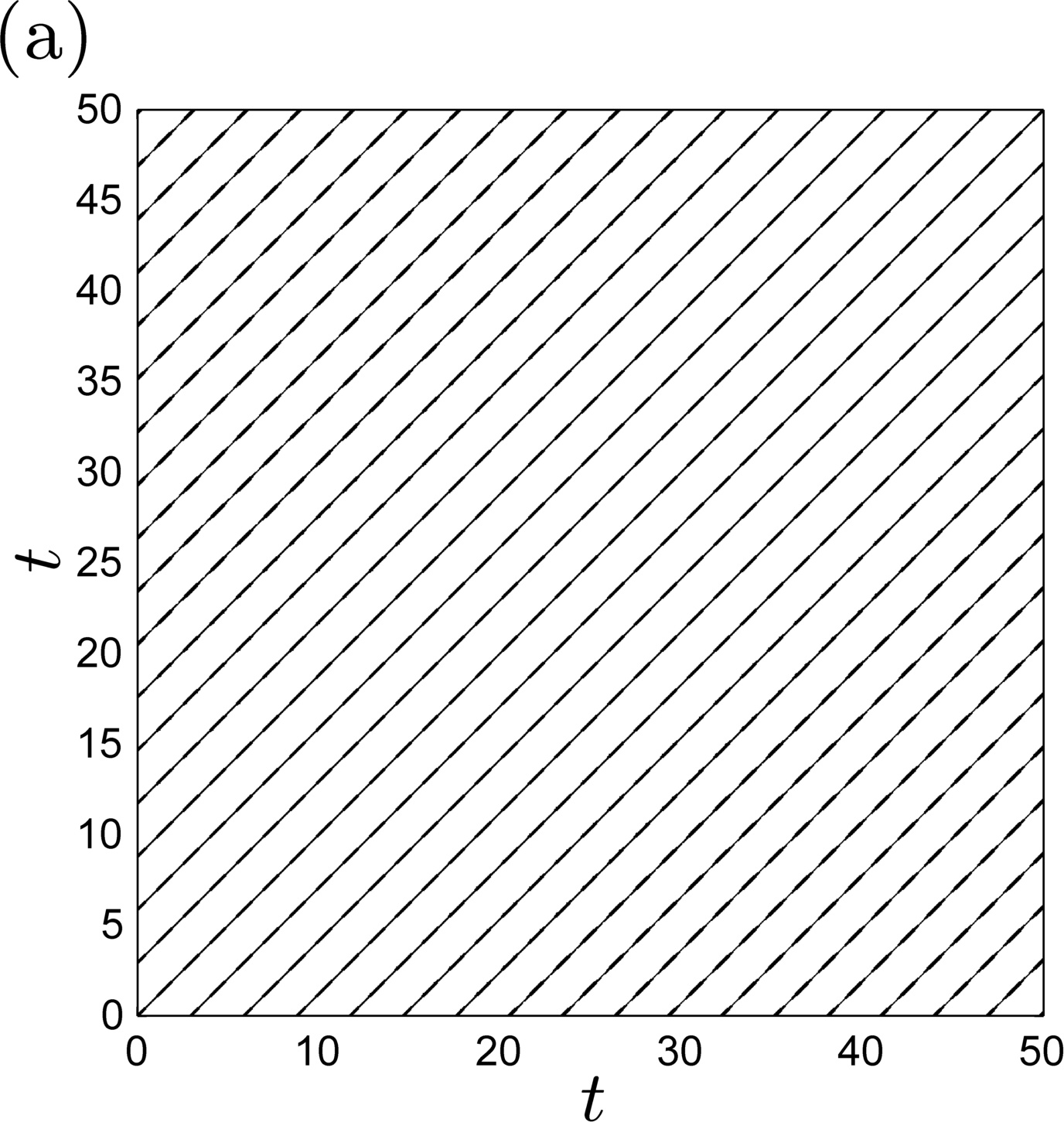
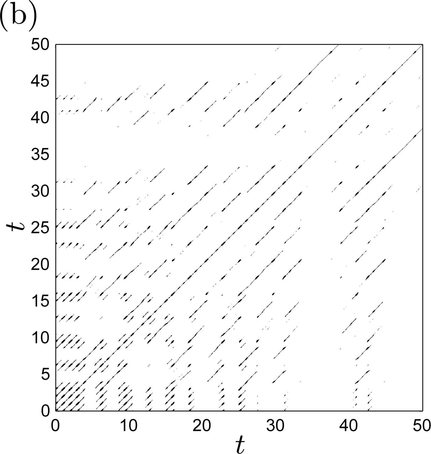
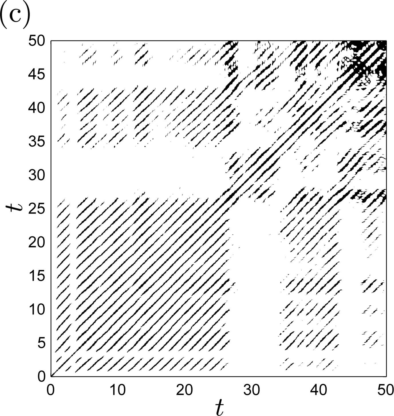
Figure 1: Recurrence plot for: (a) directly-truncated four-wave model of equation (29), (b) beatified four-wave model of equation (63), and (c) directly-truncated $272$-wave model obtained from equation (21).

Figure 1 displays the recurrence plot for the directly-truncated four-wave model, given by equation (29), with initial conditions $\mu_{\alpha,0}(0)=0$, $\mu_{0,\beta}(0)=0$, $\mu_{\alpha,\beta}(0)=(1+\mathrm{i}){\times}10^{-3}$, and $\mu_{\alpha,-\beta}(0)=(1-\mathrm{i}){\times}10^{-3}$. In this particular case, for evaluating the recurrence matrix of definition (68), we have used the time series $x(t)=\hat{\mu}(t)$. Interestingly, for an eight-dimensional dynamical system with only two known constants of motion, figure 1 portrays the typical pattern associated with periodic or quasi-periodic trajectories.

In figure 1, we present the recurrence plot for the beatified four-wave model, described by equation (63). Accordingly, in calculating the recurrence matrix, we have used the time series $x(t)=\hat{\eta}(t)$. Due to the near-identity nature of transformation (40), for simplicity, we have employed the same initial conditions of figure 1, that is, $\hat{\eta}(0)=\hat{\mu}(0)$. Unlike in the case of the directly-truncated four-wave model, figure 1 depicts the characteristic pattern of a chaotic time series, as expected from an arbitrarily chosen trajectory of an eight-dimensional Hamiltonian system with only one usual constant of motion and two Casimir invariants.

Figure 1 shows the recurrence plot for a directly truncated model obtained from equation (21) by retaining $544$ complex amplitudes or, equivalently, $272$ independent spatial wave modes. However, in the evaluation of the recurrence matrix, we have used only the time series of the eight coefficients indicated in equation (25); that is, $x(t)=\hat{\mu}(t)$. The initial values for the four dominant waves are again the same as those for figure 1, while the amplitudes of the other spatial modes are initially zero. As seen in the figure 1, the $272$-wave model also exhibits the recurrence pattern associated with chaotic trajectories.

Therefore, by considering that the $272$-wave model represents the most accurate description of the Euler’s equation among the three dynamical systems depicted in figure 1, we conclude that the beatified four-wave model presents a better qualitative characterization of the vorticity field’s overall behavior in comparison with the directly-truncated four-wave model, since figure 1 does not exhibit the recurrence pattern of a chaotic trajectory, as expected from figure 1.

Although the recurrence patterns in the figures 1 and 1 are not exactly identical, as expected from such different truncation procedures, we observe that the beatified four-wave model is able to reproduce many features of the $272$-wave model, such as intermittency, which is characterized by vertical and horizontal white stripes in the recurrence plot.

7 Summary and conclusion

The main purpose of this paper is to describe a method for extracting Hamiltonian systems of finite dimension from a class of Hamiltonian field theories with Poisson brackets of the form of (6), as described in section 2. The method was exemplified by considering a four-wave truncation of Euler’s equation for two-dimensional vortex dynamics. In section 3 we described a direct method of truncation, one that produces equations that are energy conserving but not guaranteed to be Hamiltonian. Sections 4 and 5 contain the main results of the paper, the description of the method of beatification followed by truncation. This was applied to Euler’s equation to produce our Hamiltonian four-wave example. Lastly, in section 6 we briefly used numerics and recurrence plots to compare our Hamiltonian four-wave model with the non-Hamiltonian version.

Clearly there are many applications possible for our methodology developed here, since the class of systems of section 2 includes many models from geophysical fluid dynamics and plasma physics. Moreover, it is clear that the ideas pertain to more complicated Hamiltonian models such as those with more field variables, as are common in plasma physics modeling (see e.g.  Ref.  52), three-dimensional magnetofluid models (see e.g. Ref.  53), and sophisticated kinetic theories (see e.g.  Ref.  54). In addition, one could retain more waves in the truncation, use an alternative basis other than Fourier, and proceed to higher order in the beatification procedure in order to capture higher degree of nonlinearity and more complete dynamics. Because beatification yields a Poisson bracket that is independent of the dynamical variable, conventional structure preserving numerical methods, such as symplectic integrators, could be implemented.

Appendix A Beatification to second order

In this appendix we present the calculations leading to the beatified Poisson bracket of equation (48). The operators $\mathcal{J}$, $D$, and $D^{{}^{{\dagger}}}$ defined by expressions (7), (41), and (46), respectively, satisfy various identities a few of which we will use. First, the operators $\mathcal{J}$ and $D^{{\dagger}}$ satisfy Leibniz rules, i.e.,

$$\mathcal{J}(f)gh=g\mathcal{J}(f)h+h\mathcal{J}(f)g\,,$$ (69a)

$$\mathcal{J}(fg)h=f\mathcal{J}(g)h+g\mathcal{J}(f)h\,,$$ (69b)

$$D^{{}^{{\dagger}}}fg=gD^{{\dagger}}f+fD^{{\dagger}}g\,,$$ (69c)

which are true for arbitrary functions $f$, $g$, and $h$ defined on the domain $\mathcal{D}$. Second, the operators $\mathcal{J}$, $D$, and $D^{{\dagger}}$ satisfy the following interesting identity:

$$Df\mathcal{J}(\omega_{0})g=-\mathcal{J}(f)g-\mathcal{J}(\omega_{0})f{D^{{\dagger}}}g\,,$$ (70)

which holds for any functions $f$ and $g$, and also any reference state $\omega_{0}$ that is used in the definition of the operator $D$.

Inserting (44) and its counterpart for a functional $G$ into (13), then flipping the operator $\mathcal{S}$, gives the following expression for the Poisson operator acting on an arbitrary function $f$:

$$\mathcal{S}^{{}^{{\dagger}}}\mathcal{J}_{\varepsilon}(\mu)\mathcal{S}f= \left[1+\varepsilon D\mu+\frac{\varepsilon^{2}}{2}D^{2}\mu^{2}\right]\left[\mathcal{J}(\omega_{0})+\varepsilon\mathcal{J}(\mu)\right]\left[1+\varepsilon\mu D^{{\dagger}}+\frac{\varepsilon^{2}}{2}\mu^{2}(D^{{\dagger}})^{2}\right]f$$ (71)

$$= \;\mathcal{J}(\omega_{0})f+\varepsilon\left[\mathcal{J}(\mu)+D\mu\mathcal{J}(\omega_{0})+\mathcal{J}(\omega_{0})\mu D^{{\dagger}}\right]f$$

$$+\varepsilon^{2}\left[D\mu\mathcal{J}(\mu)+\mathcal{J}(\mu)\mu D^{{\dagger}}+D\mu\mathcal{J}(\omega_{0})\mu D^{{\dagger}}\right.$$

$$\left.+\frac{1}{2}D^{2}\mu^{2}\mathcal{J}(\omega_{0})+\frac{1}{2}\mathcal{J}(\omega_{0})\mu^{2}(D^{{\dagger}})^{2}\right]f+O(\varepsilon^{3})\,.$$

Applying the identity (70) to the middle order $\varepsilon$ term gives

$$D\mu\mathcal{J}(\omega_{0})f=-\mathcal{J}(\mu)f-\mathcal{J}(\omega_{0})\mu{D^{{\dagger}}}f\,.$$ (72)

Thus, this term cancels the other two order $\varepsilon$ terms, as desired.

Now consider the terms of order $\varepsilon^{2}$, in particular we manipulate two such terms,

$$\begin{aligned} D\mu\mathcal{J}(\omega_{0})\mu{D^{{\dagger}}}f&=-\mathcal{J}(\mu)\mu{D^{{\dagger}}}f-\mathcal{J}(\omega_{0})\mu{D^{{\dagger}}}\mu{D^{{\dagger}}}f\,,\end{aligned}$$ (73a)

$$\begin{aligned} D^{2}\frac{\mu^{2}}{2}\mathcal{J}(\omega_{0})f&=-\frac{1}{2}D\mathcal{J}(\mu^{2})f-D\mathcal{J}(\omega_{0})\frac{\mu^{2}}{2}{D^{{\dagger}}}f\\ &=-D\mu\mathcal{J}(\mu)f+\mathcal{J}(\omega_{0}){D^{{\dagger}}}\frac{\mu^{2}}{2}{D^{{\dagger}}}f\,,\end{aligned}$$ (73b)

where all of the steps above follow from identities (69b) and (70). Using the results of (73a) and (73b) all of the $\varepsilon^{2}$ terms of (71) sum as follows:

$$\mathcal{J}(\omega_{0})\left(\frac{\mu^{2}}{2}D^{{\dagger}}+{D^{{\dagger}}}\frac{\mu^{2}}{2}-\mu{D^{{\dagger}}}\mu\right){D^{{\dagger}}}f\equiv 0\,,$$ (74)

as can be readily verified with the aid of identity (69c). Thus, the transformation (40) flattens the Poisson operator to second order and we obtain the beatified bracket (48). We observe that an infinite series, for which (40) constitutes the first few terms, can be shown to flatten the bracket to all orders in a manner similar to, but different from, the construction of Ref.  55.

Appendix B Canonization

Beatification is the first step to canonization, by which we mean transformation to usual canonical variables. For the Poisson bracket of (59) this is achieved by the following coordinate change:

$$q_{1}=\mathrm{i}\sigma\rho_{\alpha}^{\frac{3}{2}}\rho_{\beta}\left(\omega_{\alpha}\omega_{\beta}^{*}\eta_{\alpha,\beta}-\omega_{\alpha}^{*}\omega_{\beta}\eta_{\alpha,\beta}^{*}+\omega_{\alpha}\omega_{\beta}\eta_{\alpha,-\beta}-\omega_{\alpha}^{*}\omega_{\beta}^{*}\eta_{\alpha,-\beta}^{*}\right),$$ (75a)

$$q_{2}=\mathrm{i}\sigma\rho_{\alpha}\rho_{\beta}^{\frac{3}{2}}\left(\omega_{\alpha}\omega_{\beta}^{*}\eta_{\alpha,\beta}^{*}-\omega_{\alpha}^{*}\omega_{\beta}\eta_{\alpha,\beta}+\omega_{\alpha}^{*}\omega_{\beta}^{*}\eta_{\alpha,-\beta}-\omega_{\alpha}\omega_{\beta}\eta_{\alpha,-\beta}^{*}\right),$$ (75b)

$$q_{3}=\sigma\frac{\rho_{\beta}\rho_{\alpha,\beta}^{\frac{3}{2}}}{\rho_{\alpha}}\left(\omega_{\beta}^{*}\eta_{0,\beta}+\omega_{\beta}\eta_{0,\beta}^{*}\right)-\sigma\frac{\rho_{\alpha}\rho_{\alpha,\beta}^{\frac{3}{2}}}{\rho_{\beta}}\left(\omega_{\alpha}^{*}\eta_{\alpha,0}+\omega_{\alpha}\eta_{\alpha,0}^{*}\right),$$ (75c)

$$p_{1}=\mathrm{i}\sigma\rho_{\alpha}^{\frac{1}{2}}\rho_{\beta}\left(\omega_{\beta}\eta_{0,\beta}-\omega_{\beta}^{*}\eta_{0,\beta}^{*}\right),$$ (75d)

$$p_{2}=\mathrm{i}\sigma\rho_{\alpha}\rho_{\beta}^{\frac{1}{2}}\left(\omega_{\alpha}\eta_{\alpha,0}-\omega_{\alpha}^{*}\eta_{\alpha,0}^{*}\right),$$ (75e)

$$p_{3}=\sigma\rho_{\alpha}\rho_{\beta}\rho_{\alpha,\beta}^{\frac{1}{2}}\left(\omega_{\alpha}\omega_{\beta}^{*}\eta_{\alpha,-\beta}+\omega_{\alpha}^{*}\omega_{\beta}\eta_{\alpha,-\beta}^{*}-\omega_{\alpha}\omega_{\beta}\eta_{\alpha,\beta}-\omega_{\alpha}^{*}\omega_{\beta}^{*}\eta_{\alpha,\beta}^{*}\right),$$ (75f)

$$c_{1}=\rho_{\alpha,\beta}\left(\omega_{\alpha}^{*}\eta_{\alpha,0}+\omega_{\beta}^{*}\eta_{0,\beta}+\omega_{\alpha}\eta_{\alpha,0}^{*}+\omega_{\beta}\eta_{0,\beta}^{*}\right),$$ (75g)

$$c_{2}=\rho_{\alpha}\rho_{\beta}\left(\omega_{\alpha}^{*}\omega_{\beta}^{*}\eta_{\alpha,\beta}+\omega_{\alpha}^{*}\omega_{\beta}\eta_{\alpha,-\beta}+\omega_{\alpha}\omega_{\beta}\eta_{\alpha,\beta}^{*}+\omega_{\alpha}\omega_{\beta}^{*}\eta_{\alpha,-\beta}^{*}\right),$$ (75h)

where $(q_{j},p_{j})$, for $j=1,2,3$, are real canonically conjugate pairs, the variables $c_{1}$ and $c_{2}$ are equivalent to the two Casimir invariants $\bar{\mathcal{C}}^{(2)}_{\hat{\eta}}$ and $\bar{\mathcal{C}}^{(3)}_{\hat{\eta}}$, and we have defined the constants $\sigma={1}/{(2\pi}{\sqrt{\alpha\beta}})$, $\rho_{j}=1/\sqrt{\omega_{j}^{2}+(\omega_{j}^{*})^{2}}$, for $j=\alpha,\beta$, and $\rho_{\alpha,\beta}=1/\sqrt{\omega_{\alpha}^{2}+(\omega_{\alpha}^{*})^{2}+\omega_{\beta}^{2}+(\omega_{\beta}^{*})^{2}}$.

Upon writing

$$\hat{\eta}_{c}=(q_{1},\,q_{2},\,q_{3},\,p_{1},\,p_{2},\,p_{3},\,c_{1},\,c_{2})\,,$$ (76)

the Poisson bracket for the beatified four-wave model becomes

$$\{f,g\}_{\hat{\eta}_{c}}=\left(\frac{\partial f}{\partial\hat{\eta}_{c}}\right)^{T}\!\!\!\cdot J_{\hat{\eta}_{c}}\cdot\left(\frac{\partial g}{\partial\hat{\eta}_{c}}\right)\,,$$ (77)

with canonized Poisson matrix,

$$J_{\hat{\eta}_{c}}=\left(\begin{array}[]{c c}J_{c}&0_{6\times 2}\\ 0_{2\times 6}&0_{2\times 2}\end{array}\right),$$ (78)

where the block $J_{c}$ is given by (39) with $r=3$. The form of (78) reveals that an ordinary three degree-of-freedom Hamiltonian system lives in the original eight dimensional phase space. Using the Casimir invariants, a consequence of the degeneracy of Poisson matrix, as coordinates separated out the superfluous dimensions, and the canonization transformation of this appendix put the remaining six coordinates into canonical form.

References

- 1 A. Arakawa. J. Comp. Phys., 1:119–143, 1966.
- 2 A. Arakawa and V. R. Lamb. Mon. Weather Rev., 109:18–36, 1981.
- 3 R. Salmon and L. D. Talley. J. Comp. Phys., 83:247–259, 1989.
- 4 B. Cockburn and C.-W. Shu. Math. Model. Numer. Anal., 25:337–361, 1991.
- 5 Y. Cheng, I. M. Gamba, and P. J. Morrison. J. Sci. Comput., 56:319–349, 2013.
- 6 P. J. Morrison and J. M. Greene. Phys. Rev. Lett., 45:790–794, 1980.
- 7 P. J. Morrison. Rev. Mod. Phys., 70:467–521, 1998.
- 8 J. Weiland and H. Wilhelmsson. Coherent Nonlinear Interaction of Waves in Plasmas. Pergamon Press, New York, 1977.
- 9 J.-M. Wersinger, J. M. Finn, and E. Ott. Phys. Rev. Lett., 44:453–456, 1980.
- 10 S. R. Lopes and A. C.-L. Chian. Phys. Rev. E, 54:170–174, 1996.
- 11 R. Sugihara. Phys. Fluids, 11:178–184, 1968.
- 12 K. S. Karplyuk, V. N. Oraevskii, and V. P. Pavlenko. Plasma Physics, 15:113–124, 1973.
- 13 J. G. Turner. Physica Scrip., 21:185–190, 1980.
- 14 F. Verheest. J. Phys. A, 15:1041–1050, 1982.
- 15 F. J. Romeiras. Phys. Lett. A, 93:227–229, 1983.
- 16 A. C.-L. Chian, S. R. Lopes, and J. R. Abalde. Physica D, 99:269–275, 1996.
- 17 R. Pakter, S. R. Lopes, and R. L. Viana. Physica D, 110:277–288, 1997.
- 18 J. G. Charney. J. Atmos. Sci., 28:1087–1095, 1971.
- 19 A. Hasegawa and K. Mima. Phys. Fluids, 21:87–92, 1978.
- 20 C. P. Connaughton, B. T. Nadiga, S.V. Nazarenko, and B. E. Quinn. J. Fluid Mech., 654:207–231, 2010.
- 21 C. N. Lashmore-Davies, D. R. McCarthy, and A. Thyagaraja. Phys. Plasmas, 8:5121–5133, 2001.
- 22 C. N. Lashmore-Davies, A. Thyagaraja, and D. R. McCarthy. Phys. Plasmas, 12:122304, 2005.
- 23 R. A. Kolesnikov and J. A. Krommes. Phys. Rev. Lett., 94:235002, 2005.
- 24 J.P. Denier and J.S. Frederiksen, editors. volume 6 of World Scientific Lecture Notes in Complex Systems. World Scientific, 2007.
- 25 P. J. Morrison. Phys. Plasmas, 12:058102, 2005.
- 26 E. Tassi, P. J. Morrison, F. L. Waelbroeck, and D. Grasso. Plasma Phys. Control. Fusion, 50:085014, 2008.
- 27 C. S. Kueny and P. J. Morrison. Phys. Plasmas, 2:1926–1940, 1995.
- 28 C. S. Kueny and P. J. Morrison. Phys. Plasmas, 2:4149–4160, 1995.
- 29 V. E. Zakharov and L. A. Ostrovsky. Physica D, 238:540548, 2009.
- 30 P. Iorra, S. Marini, E. Peter, R. Pakter, and F.B. Rizzato. Physica A, 436:686–693, 2015.
- 31 P. J. Morrison. Hamiltonian field description of the two-dimensional vortex fluids and guiding center plasmas. Technical Report PPPL–1783, Princeton University Plasma Physics Laboratory, Princeton, New Jersey, March 1981.
- 32 P. J. Morrison. AIP Conf. Proc., 88:13–46, 1982.
- 33 P. J. Morrison and J. Vanneste. Weakly nonlinear dynamics in noncanonical Hamiltonian systems with applications to fluids and plasmas. Preprint: arXiv:1512.07230v1 [physics.plasm-ph].
- 34 P. J. Olver. Contemp. Math, 28:231–249, 1984.
- 35 P. J. Olver. Hamiltonian and non-Hamiltonian models for water waves. In P. G. Ciarlet and M. Roseau, editors, Trends and Applications of Pure Mathematics to Mechanics, pages 273–290. Springer, Berlin, 1984.
- 36 Y. M. Vorob’ev and M. V. Karasev. Funct. Anal. Appl., 22:1–9, 1988.
- 37 R. Flores-Espinoza. The lie transform method for perturbations of contravariant antisymmetric tensor fields and its applications to hamiltonian dynamics. Preprint: arXiv:1308.0307v1 [math-ph].
- 38 J. A. Schouten. Convegno Internazionale di Geometria Differenziale, pages 1–7, 1953.
- 39 P. J. Morrison. Hamiltonian description of fluid and plasma systems with continuous spectra. In Nonlinear Processes in Geophysical Fluid Dynamics, pages 53–69, Dordrecht, 2003. Kluwer.
- 40 P. J. Morrison. Phys. Lett. A, 80:383–386, 1980.
- 41 E. Tassi, C. Chandre, and P. J. Morrison. Phys. Plasmas, 16:082301, 2009.
- 42 D. Montgomery and R. Kraichnan. Rep. Prog. Phys., 43:547–619, 1979.
- 43 R. Jost. Rev. Mod. Phys., 36:572–579, 1964.
- 44 R. Abraham and J. E. Marsden. Foundations of Mechanics. Addison-Wesley, Redwood City, CA., 1987.
- 45 E. Sudarshan and N. Makunda. Classical Dynamics: A Modern Perspective. Wiley, New York, 1974.
- 46 A. Weinstein. J. Diff. Geom., 18:523–557, 1983. Erratum: ibid. 22:255, 1985.
- 47 C. Chandre, P. J. Morrison, and E. Tassi. Phys. Lett. A, 378:956–959, 2014.
- 48 P. J. Morrison and J. M. Greene. Phys. Rev. Lett., 48:569, 1982.
- 49 T. F. Viscondi and M. A. M. de Aguiar. J. Math. Phys., 52:052104, 2011.
- 50 T. F. Viscondi and M. A. M. de Aguiar. J. Chem. Phys., 134:234105, 2011.
- 51 N. Marwan, M. C. Romano, M. Thiel, and J. Kurths. Phys. Rep., 438:237–329, 2007.
- 52 Jean-Luc Thiffeault and P. J. Morrison. Physica D, 136:205–244, 2000.
- 53 M. Lingam, P. J. Morrison, and G. Miloshevich. Phys. Plasmas, 22:072111, 2015.
- 54 J. Burby, A. Brizard, P. J. Morrison, and H. Qin. Phys. Lett. A, 379:2073–2077, 2015.
- 55 H. Ye, P. J. Morrison, and J. D. Crawford. Phys. Lett. A, 156:96–100, 1991.