A spatial compositional model (SCM) for linear unmixing and endmember uncertainty estimation

Abstract

The normal compositional model (NCM) has been extensively used in hyperspectral unmixing. However, most of the previous research has focused on estimation of endmembers and/or their variability. Also, little work has employed spatial information in NCM. In this paper, we show that NCM can be used for calculating the uncertainty of the estimated endmembers with spatial priors incorporated for better unmixing. This results in a spatial compositional model (SCM) which features (i) spatial priors that force neighboring abundances to be similar based on their pixel similarity and (ii) a posterior that is obtained from a likelihood model which does not assume pixel independence. The resulting algorithm turns out to be easy to implement and efficient to run. We compared SCM with current state-of-the-art algorithms on synthetic and real images. The results show that SCM can in the main provide more accurate endmembers and abundances. Moreover, the estimated uncertainty can serve as a prediction of endmember error under certain conditions.

1 Introduction

Hyperspectral image unmixing has received wide attention in the remote sensing, signal and image processing communities [18, 6]. The widely researched model in this area is the linear mixing model (LMM). Assume we have a hyperspectral image $I\left(\mathbf{x}\right):\mathcal{D}\to L^{2}\left(\mathbb{R}^{+}\right)$ where $\mathcal{D}\subset\mathbb{R}^{2}$ is the image domain with $L^{2}\left(\mathbb{R}^{+}\right)$ denoting the space of square integrable functions on the positive part of the real line. LMM assumes that the spectral measurement of each pixel $g\left(\mathbf{x},\lambda\right)$, with $\lambda$ being the wavelength, is a non-negative linear combination of the spectral signature of some pure materials, called endmembers, $f_{j}\left(\lambda\right):\mathbb{R}^{+}\to\mathbb{R}^{+}$. The governing equation is

$$g\left(\mathbf{x},\lambda\right)=\sum_{j=1}^{M}f_{j}\left(\lambda\right)\alpha_{j}\left(\mathbf{x}\right)+n\left(\mathbf{x},\lambda\right)$$ (1)

$$\forall\mathbf{x}\in\mathcal{D},\,\sum_{j=1}^{M}\alpha_{j}\left(\mathbf{x}\right)=1$$

where $M$ is the number of endmembers, $\alpha_{j}\left(\mathbf{x}\right):\mathcal{D}\to\mathbb{R}^{+}$ is the fractional abundance map of the jth endmember and satisfies the positivity and sum-to-one (simplex) constraints, and $n\left(\mathbf{x},\lambda\right):\mathcal{D}\times\mathbb{R}^{+}\to\mathbb{R}$ is a small, additive perturbation (noise). As a result, the pixels generated by this model form a simplex in an infinite dimensional vector space whose vertices are the endmembers. If we discretize $f_{j}\left(\lambda\right)$ into $B$ bands and get $\mathbf{m}_{j}\in\mathbb{R}^{B}$ as the discretized value, and further discretize $\mathcal{D}$ into $N$ locations, equation (1) states that the spectrum of the ith pixel can be represented by

$$\mathbf{y}_{i}=\mathbf{M}^{T}\boldsymbol{\alpha}_{i}+\mathbf{n}_{i}$$

where $\mathbf{M}=\left[\mathbf{m}_{1},...,\mathbf{m}_{M}\right]^{T}$, $\boldsymbol{\alpha}_{i}=\left[\alpha_{i1},...,\alpha_{iM}\right]^{T}$, $\mathbf{y}_{i}\in\mathbb{R}^{B}$, $\mathbf{n}_{i}\in\mathbb{R}^{B}$. Combining the above equation for all the pixels, we have the following equation for LMM:

$$\mathbf{Y=AM+N}$$ (2)

where $\mathbf{Y}\in\mathbb{R}^{N\times B}$, $\mathbf{A}\in\mathbb{R}^{N\times M}$, $\mathbf{M}\in\mathbb{R}^{M\times B}$, $\mathbf{N}\in\mathbb{R}^{N\times B}$.

The linear unmixing problem is to retrieve $\mathbf{A}$ and $\mathbf{M}$ given $\mathbf{Y}$. This is an ill-posed inverse problem as it can have an infinite number of solutions. Figure 1 shows the difficulties stemming from this underdetermined nature: Figure 1(a) shows the pixels (gray area) generated by 2 endmembers $\mathbf{m}_{1}$, $\mathbf{m}_{2}$ with $\boldsymbol{\alpha}=(0.5,0.5)^{T}$ for all pixels. Clearly it is not possible to retrieve $\mathbf{A}$ and $\mathbf{M}$ given $\mathbf{Y}$ in this case. As shown in the figure, we can have $\mathbf{m}_{1}^{\prime}$, $\mathbf{m}_{2}^{\prime}$ or $\mathbf{m}_{1}^{\prime\prime}$, $\mathbf{m}_{2}^{\prime\prime}$ generate the same pixels. In fact, we can have the whole Euclidean space for the endmembers. In Figure 1(b), the abundances $\boldsymbol{\alpha}$ ranges from $(0.7,0.3)$ to $(0.2,0.8)$. Here, we can determine that the endmembers should lie in a line that fits the pixels. However, we still cannot determine the specific position of the endmembers without other information. For example, $\mathbf{m}_{1}^{\prime}$, $\mathbf{m}_{2}^{\prime}$ or $\mathbf{m}_{1}^{\prime\prime}$, $\mathbf{m}_{2}^{\prime\prime}$ can both serve as the endmember set. In Figure 1(c), we have the information that the abundances range from $(1,0)$ to $(0,1)$. Now we can find the endmembers as we are not only given the line, but also the relative position of the endmembers to the boundary of the pixels. This is the only case where we have a unique solution which corresponds to the original endmembers. The intuition (stemming from this observation) that the endmembers should tightly surround the pixels has been extensively used in the literature, in the form of minimal volume [21], pure pixels [22], or pairwise closeness [4, 27]. Figure 1(d) shows another interesting problem. Suppose we have two endmember sets, $\mathbf{m}_{1}$, $\mathbf{m}_{2}$ and $\mathbf{m}_{3}$, $\mathbf{m}_{4}$ and we can find them. How can we then determine the abundance $\boldsymbol{\alpha}$ of the pixel in the intersection given these endmembers? Should it be a linear combination of $\mathbf{m}_{1}$ and $\mathbf{m}_{2}$ or a linear combination of $\mathbf{m}_{3}$ and $\mathbf{m}_{4}$, or a combination of all of them? However, if the pixels from an endmember set lies in one region while those from the other set lie in another region, the abundances in the intersection can by easily identified by the spatial location. This implies that spatial information should be used in the unmixing process.

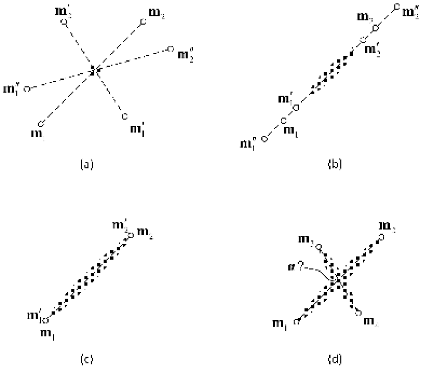
Figure 1: Difficulties in the linear unmixing problem: $\mathbf{m}_{1}$, $\mathbf{m}_{2}$ are the endmembers that generate the pixel data. $\mathbf{m}_{1}^{\prime}$, $\mathbf{m}_{2}^{\prime}$ and $\mathbf{m}_{1}^{\prime\prime}$, $\mathbf{m}_{2}^{\prime\prime}$ are the possible endmembers that can be inferred from the data. In (a), (b) are 2 cases where the true endmembers can not be estimated while (c) contains a case where they can be estimated under some assumptions. In (d), we show the importance of spatial location to abundance estimation.

The methods developed to solve this problem may be mainly categorized into geometrical, statistical and sparse regression based approaches [6]. For example, vertex component analysis (VCA) assumes the endmembers are present in the image pixels [22], iterative constrained endmembers (ICE) minimizes the least squares error under the pairwise closeness constraint [4], minimum volume constrained nonnegative matrix factorization (MVC-NMF) minimizes the same error and the volume of the simplex [21], piecewise convex multiple-model endmember detection (PCOMMEND) minimizes the least square errors of separate convex sets [27].

Besides these methods that rely only on independent pixels, some recent work introduced spatial information to aid the unmixing process [17, 11, 16]. For example, in [17] two smoothness terms for abundances and endmembers were proposed to utilize the spatial information in terms of wavelength proximity and pixel location. In [11] a Markov Random Field (MRF), Potts-Markov model, was used to model the partitioning of the image that can help the unmixing process. Sampling methods were used to infer the unknown parameters. In [16], a constraint that minimizes the $L_{1}$ norm of the differences between neighboring abundances was proposed to impose spatial correlation.

Another type of method is based on modeling the likelihood using Gaussian density functions, also known as the normal compositional model (NCM) [9, 10, 26, 24, 29]. The earliest application of NCM to hyperspectral unmixing can be traced back to [24], where a maximal likelihood estimation (MLE) approach was presented for NCM endmember extraction. In [9, 10], priors (mainly uniform distributions) were imposed on endmembers and abundances with sampling methods used to maximize the posterior. They assumed the variance of each wavelength was independent and estimated one parameter of variability for each endmember. In [26], a Dirichlet prior distribution on the abundances was used. However, in their model the covariance matrices of the endmembers are assumed to be known instead of being unknown parameters to be estimated. In [29], a more complicated NCM without the assumption of independence of each wavelength was proposed. They maximize the posterior using particle swarm optimization based expectation maximization.

However, there is little work on estimating the model uncertainty of the endmembers directly from the linear mixing model. That is, given the pixel data and an estimated endmember set, the endmember estimates may have residual uncertainty. For example, Figure 2 shows 3 possible estimated endmember sets on a synthetic dataset when $B=2$. We can expect the endmember set $\mathbf{m}_{1},\mathbf{m}_{2},\mathbf{m}_{3}$ to have a small uncertainty since they fit the pixels very well. Allowing them to move around may ruin the fitting. $\mathbf{m}_{1}^{\prime},\mathbf{m}_{2}^{\prime},\mathbf{m}_{3}^{\prime}$ are located within the pixels. They should have a large uncertainty because they can move around more freely to better fit the pixels. For $\mathbf{m}_{1}^{\prime\prime},\mathbf{m}_{2}^{\prime\prime},\mathbf{m}_{3}^{\prime\prime}$, the uncertainty is ambiguous because they have already fitted the pixels very well while they may also move around to some degree. Hence we will not consider the uncertainty in this case in the present work.

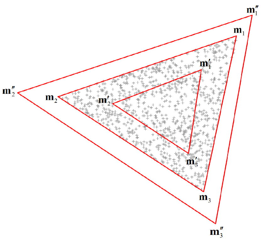
Figure 2: Model uncertainty of the estimated endmembers at different positions. Intuitively, $\mathbf{m}_{1},\mathbf{m}_{2},\mathbf{m}_{3}$ should have a small uncertainty while the uncertainty of $\mathbf{m}_{1}^{\prime},\mathbf{m}_{2}^{\prime},\mathbf{m}_{3}^{\prime}$ should be large. The uncertainty of $\mathbf{m}_{1}^{\prime\prime},\mathbf{m}_{2}^{\prime\prime},\mathbf{m}_{3}^{\prime\prime}$ will not be discussed here due to its ambiguity.

The above intuition implies that the uncertainty may reflect the error of endmembers. To show how this intuition formally works in NCM, assume a simple case that an endmember $\mathbf{m}\in\mathbb{R}^{2}$ follows a Gaussian distribution centered at $\mathbf{r}\in\mathbb{R}^{2}$ with covariance matrix $\boldsymbol{\Sigma}\in\mathbb{R}^{2\times 2}$:

$$p\left(\mathbf{m}\right)=\mathcal{N}\left(\mathbf{m}|\mathbf{r},\boldsymbol{\Sigma}\right).$$

Suppose $\mathbf{m}$ is given and $\mathbf{r}$ has been estimated with $\mathbf{m}\neq\mathbf{r}$. We want to find $\boldsymbol{\Sigma}$ using maximum likelihood estimation (MLE). Maximizing $p\left(\mathbf{m}\right)$ is equivalent to minimizing

$$-\log p(\mathbf{m})=\frac{1}{2}\text{log}\left|\boldsymbol{\Sigma}\right|+\frac{1}{2}\left(\mathbf{m}-\mathbf{r}\right)^{T}\boldsymbol{\Sigma}^{-1}\left(\mathbf{m}-\mathbf{r}\right).$$

Let $\boldsymbol{\Sigma}=\mathbf{U}\text{diag}\left(\sigma_{1}^{2},\sigma_{2}^{2}\right)\mathbf{U}^{T}$, $\sigma_{1}>0$, $\sigma_{2}>0$ be the eigendecomposition, then the minimization problem above becomes

$$\text{log}\sigma_{1}+\text{log}\sigma_{2}+\frac{1}{2}\sigma_{1}^{-2}z_{1}^{2}+\frac{1}{2}\sigma_{2}^{-2}z_{2}^{2}$$

where $\mathbf{z}=\left(z_{1},z_{2}\right)^{T}=\mathbf{U}^{T}\left(\mathbf{m}-\mathbf{r}\right)$. When the eigenvector in $\mathbf{U}$ is not perpendicular to $\mathbf{m}-\mathbf{r}$, i.e. $z_{1}\neq 0$, $z_{2}\neq 0$, the minimization can be achieved by setting the derivatives with respect to $\sigma_{1}$ and $\sigma_{2}$ to 0, which leads to

$$\sigma_{1}=\left|z_{1}\right|,\,\sigma_{2}=\left|z_{2}\right|.$$

However, this is not the global minimum because if one eigenvector in $\mathbf{U}$ is perpendicular to $\mathbf{m}-\mathbf{r}$ (the other being parallel), say $z_{2}=0$, $z_{1}=\|\mathbf{m}-\mathbf{r}\|$, $\sigma_{2}$ can be arbitrarily close to 0 such that $\text{log}\sigma_{2}$ goes to negative infinity. Assume $\sigma_{i}\geq\epsilon$ for a small positive $\epsilon$ to make a solution exist, then the global minimum lies at $\sigma_{1}=\|\mathbf{m}-\mathbf{r}\|$, $\sigma_{2}=\epsilon$. Therefore, we can see that the MLE estimated matrix $\boldsymbol{\Sigma}$ has the square root of its largest eigenvalue equal to $\|\mathbf{m}-\mathbf{r}\|$ while its eigenvector is parallel to $\mathbf{m}-\mathbf{r}$. For our formulation (2), assume $\mathbf{M}$ follows a Gaussian distribution with centers in $\mathbf{R}$. We then propose a fundamental question:

• Given $\mathbf{Y}$, can we find the covariance matrices (uncertainty) that measure the difference between the estimated endmembers $\mathbf{R}$ and the ground truth $\mathbf{M}$?

If the answer is yes, we have a measure to predict the error without knowing the ground truth. This paper attempts to find such covariance matrices.

The previous NCMs did not solve this problem. The covariance matrices from the previous NCMs represent the endmember variability which arises from the assumption that the endmember set used for linearly generating a pixel may vary per pixel due to atmospheric, environmental, temporal factors and intrinsic variability in a material [28]. We explain the difference between these two concepts, uncertainty and variability, here by first summarizing the previous NCMs. Suppose the $j$th endmember follows a Gaussian distribution centered at $\mathbf{r}_{j}\in\mathbb{R}^{B}$ with covariance matrix $\boldsymbol{\Sigma}_{j}$:

$$p(\mathbf{m}_{j})=\mathcal{N}\left(\mathbf{m}_{j}|\mathbf{r}_{j},\boldsymbol{\Sigma}_{j}\right).$$

Assuming the endmembers to be independent, the random variable transformation $\mathbf{y}_{i}=\mathbf{M}^{T}\boldsymbol{\alpha}_{i}$ for each pixel suggests that the probability density function of $\mathbf{y}_{i}$ can be derived as

$$p(\mathbf{y}_{i})=\mathcal{N}\left(\mathbf{y}_{i}|\mathbf{R}^{T}\boldsymbol{\alpha}_{i},\sum_{j=1}^{M}\alpha_{ij}^{2}\boldsymbol{\Sigma}_{j}\right)$$

where $\mathbf{R}=\left[\mathbf{r}_{1},...,\mathbf{r}_{M}\right]^{T}$. Then, NCM assumes the pixels are independent and obtains the density function of $\mathbf{Y}$ as

$$p(\mathbf{Y})=\prod_{i=1}^{N}p(\mathbf{y}_{i})$$ (3)

which is another Gaussian distribution with a block diagonal covariance matrix. The estimation of $\mathbf{r}_{j}$ and $\boldsymbol{\Sigma}_{j}$ is handled differently in different works.

To estimate the uncertainty however, we can not assume the pixels to be independent. To see this, suppose $B=1$. Then we have $\mathbf{M}\in\mathbb{R}^{M}$, $\mathbf{R}\in\mathbb{R}^{M}$, $\mathbf{Y}\in\mathbb{R}^{N}$ which are all vectors and the covariance matrix in (3) becomes an $N$ by $N$ diagonal matrix. The independence of endmembers suggests that the density of $\mathbf{M}$ is given by

$$p(\mathbf{M})=\mathcal{N}\left(\mathbf{M}|\mathbf{R},\boldsymbol{\Sigma}\right)$$

where $\boldsymbol{\Sigma}$ is an $M$ by $M$ diagonal matrix with each element being the variance of each endmember. The random variable transformation $\mathbf{Y}=\mathbf{A}\mathbf{M}$ indicates that the density function of $\mathbf{Y}$ does not even exist. This is because the domain of $p(\mathbf{M})$ ($\mathbb{R}^{M}$) is projected to a subspace of dimension $M$ in $\mathbb{R}^{N}$, which has measure 0 (integrating $p(\mathbf{Y})$ would give value 0). The only way to make the density function exist is to add noise, i.e., use equation (2). By assuming the noise to be Gaussian and independent for each pixel, $p(\mathbf{N})=\mathcal{N}\left(\mathbf{N}|\mathbf{0},\mu^{2}\mathbf{I}_{N}\right)$, we can see that the density function of $\mathbf{Y}$ becomes

$$p(\mathbf{Y})=\mathcal{N}\left(\mathbf{Y}|\mathbf{A}\mathbf{R},\,\mathbf{A}\boldsymbol{\Sigma}\mathbf{A}^{T}+\mu^{2}\mathbf{I}_{N}\right)$$

where the covariance matrix is not a diagonal matrix, which indicates the pixels are not independent. The general case with $B>1$ will be derived later.

In this paper, we solve the problem of estimating the model uncertainty by proposing a spatial compositional model (SCM) based on NCM without assuming independence while utilizing spatial information on the abundances. Compared to previous NCMs and methods with spatial information, our method differs in the following aspects:

1. In contrast to the previous NCMs which assume pixel independence, we estimate the full likelihood of the pixels (without the independence assumption). Hence, we can obtain the endmember uncertainty that predicts the error.

2. In the previous works, a uniform smoothness term is imposed to force every two neighboring abundances to be similar [11, 16]. In our work, the smoothness term varies locally according to pixel information. Moreover, it is in a quadratic form which entails a simple algorithm.

3. The previous works assume the covariance matrices of endmembers have a simple form, e.g. diagonal (each wavelength is independent), which neglects the correlation between wavelengths [9, 10]. Here we estimate the full covariance matrices and capture the correlations.

The resulting model can be summarized by modeling the priors on abundances based on the spatial information, the priors on endmembers based on smoothness and principles of pairwise closeness, and transforming the Gaussian probability functions to obtain the posterior which can be maximized. The final minimization problem can be solved by a simple and efficient optimization algorithm that not only provides the endmembers, the abundances, but also the uncertainty.

Notation. Throughout the paper, $\text{SPD}\left(n\right)$ denotes the set of all $n$ by $n$ symmetric positive definite matrices. We use the following notation for operations on a matrix $\mathbf{A}=\left[\mathbf{a}_{1},...,\mathbf{a}_{n}\right]$. We use $\text{Tr}\left(\mathbf{A}\right)$, $\left|\mathbf{A}\right|$, $\text{vec}\left(\mathbf{A}\right)$ to denote the trace, determinant, vectorization of $\mathbf{A}$ respectively. The vectorization operator is defined by concatenating its columns, $\text{vec}\left(\mathbf{A}\right)=\left[\mathbf{a}_{1}^{T},...,\mathbf{a}_{n}^{T}\right]^{T}$. We use $[a_{ij}]$ to denote a matrix in which the element at the $i$th row, $j$th column is $a_{ij}$. So the matrix $\left[\delta_{ij}a_{i}\right]$ is a diagonal matrix with diagonal element $a_{i}$ by defining $\delta_{ij}=1$ only when $i=j$ and 0 otherwise. We use $\mathbf{A}\geq 0$ to denote that $a_{ij}\geq 0$ given $\mathbf{A}=\left[a_{ij}\right]$. The Kronecker product between two matrices $\mathbf{A}$ and $\mathbf{B}$ is defined by $\mathbf{A}\otimes\mathbf{B}=\left[a_{ij}\mathbf{B}\right]$. We use $\|\mathbf{A}\|$, $\|\mathbf{A}\|_{F}$ as the operator norm and Frobenius norm of $\mathbf{A}$ respectively. We use $\mathbf{I}_{N}$ for the $N$ by $N$ identity matrix and $\mathbf{1}_{N}$ as an $N$ by 1 vector consisting of all 1s.

2 The Spatial Compositional Model

2.1 The hyperspectral image likelihood

We are interested in determining the uncertainty of the extracted endmembers. To achieve this, we first model the density function of $\mathbf{M}$, then use (2) to perform a random variable transformation to get the density function of $\mathbf{Y}$, and finally maximize the posterior given $\mathbf{Y}$ to find the parameters. Assuming that the endmember $\mathbf{m}_{j}$ follows a multivariate Gaussian centered at $\mathbf{r}_{j}$ with covariance matrix $\mathbf{\boldsymbol{\Sigma}}_{j}$, we have the conditional probability density function of $\mathbf{m}_{j}$:

$$p(\mathbf{m}_{j}|\mathbf{r}_{j},\boldsymbol{\Sigma}_{j})=\mathcal{N}\left(\mathbf{m}_{j}|\mathbf{r}_{j},\boldsymbol{\Sigma}_{j}\right).$$

We can also assume that the endmembers are independent, which leads to the conditional probability density function of the whole endmember set to be the product of the independent components:

$$p(\mathbf{M}|\mathbf{R},\boldsymbol{\Theta})=\mathcal{N}\left(\text{vec}(\mathbf{M}^{T})|\text{vec}(\mathbf{R}^{T}),\,[\delta_{ij}\boldsymbol{\Sigma}_{j}]\right),$$ (4)

where $\boldsymbol{\Theta}=\left\{\boldsymbol{\Sigma}_{j}\right\}$, the covariance matrix is an $MB$ by $MB$ block diagonal matrix.

From the probability density function of the endmembers in (4), we can obtain the probability density function of $\mathbf{Y}$ from the linear transformation in (2). From straightforward matrix algebra, we see that

$$\text{vec}\left((\mathbf{AM})^{T}\right) = (\mathbf{A}\otimes\mathbf{I}_{B})\text{vec}(\mathbf{M}^{T}).$$ (5)

Assuming that the noise $\mathbf{n}_{i}$ follows an independent zero mean, $\mu^{2}$ variance Gaussian at each wavelength which is independent at different locations, we have

$$p(\mathbf{N}|\mu)=\mathcal{N}\left(\text{vec}(\mathbf{N}^{T})|\mathbf{0},\,\mu^{2}\mathbf{I}_{NB}\right).$$ (6)

From the probability density functions in (6), (4) and the transformation in (5), equation (2) indicates that the conditional probability density function of $\mathbf{Y}$ can be obtained as

$$p(\mathbf{Y}|\mathbf{R},\boldsymbol{\Theta},\mathbf{A},\mu)=\mathcal{N}\left(\text{vec}(\mathbf{Y}^{T})|\boldsymbol{\mu}_{\mathbf{Y}},\boldsymbol{\Sigma}_{\mathbf{Y}}\right),$$ (7)

where

$$\boldsymbol{\mu}_{\mathbf{Y}} = (\mathbf{A}\otimes\mathbf{I}_{B})\text{vec}(\mathbf{R}^{T})$$

$$= \text{vec}\left((\mathbf{AR})^{T}\right),$$

$$\boldsymbol{\Sigma}_{\mathbf{Y}} = (\mathbf{A}\otimes\mathbf{I}_{B})[\delta_{ij}\boldsymbol{\Sigma}_{j}](\mathbf{A}\otimes\mathbf{I}_{B})^{T}+\mu^{2}\mathbf{I}_{NB}$$ (8)

$$= \left[\delta_{ij}\mu^{2}\mathbf{I}_{B}+\sum_{k=1}^{M}\alpha_{ik}\alpha_{jk}\boldsymbol{\Sigma}_{k}\right].$$

Note that the covariance matrix in (8) is not a block diagonal matrix, which means that the transformed rows in $\mathbf{Y}$ are not independent.

2.2 Modeling the priors

We model the prior probability density of $\mathbf{A}$ by assuming that $\boldsymbol{\alpha}_{i}$ is a Markov random field (MRF). That is, we treat the image grid as an undirected graph $\mathcal{G}=\left(\mathcal{V},\,\mathcal{E}\right)$ where $\mathcal{V}$ is the set of graph nodes and $\mathcal{E}$ is the set of edges. The density of the whole grid can be modeled based on a potential function of the neighboring nodes. Suppose the hyperspectral image is divided into different regions ($\mathcal{D}=\bigcup_{k=1}^{S}\Omega_{k}$, $\Omega_{i}\bigcap\Omega_{j}=\emptyset$ when $i\neq j$) with the pixels of a region showing similar reflectances, we have $S$ sets of graph nodes $\mathcal{V}_{k}$, $k=1,...,S$. Then, the prior probability density of $\mathbf{A}$ can be assumed to be in favor of smooth assignment of $\boldsymbol{\alpha}_{i}$ to all the neighboring pixels within a region, because they are more likely to be the same mixture of materials and their abundances should be similar.

Driven by this intuition, the prior probability density of $\mathbf{A}$ is modeled as

$$p(\mathbf{A}) \propto \exp\left\{-\frac{\beta_{1}}{4}\sum_{i=1}^{N}\sum_{j=1}^{N}w_{ij}\|\boldsymbol{\alpha}_{i}-\boldsymbol{\alpha}_{j}\|^{2}\right\}$$ (9)

$$= \exp\left\{-\frac{\beta_{1}}{2}\text{Tr}\left(\mathbf{A}^{T}\mathbf{L}\mathbf{A}\right)\right\},$$

where $w_{ij}$ controls the spatial intimacy between node $i$ and node $j$, $\mathbf{L}=\left[\delta_{ij}\sum_{k}w_{ik}\right]-\left[w_{ij}\right]$ where $\mathbf{L}\in\mathbb{R}^{N\times N}$ is the well known symmetric positive semidefinite graph Laplacian matrix [25]. If we have a prior segmentation result, we can set $w_{ij}$ to be 1 when node $i$ and node $j$ are neighbors that belong to the same region ${\cal V}_{k}$ and 0 otherwise. If we do not have a prior segmentation, we can use

$$w_{ij}=e^{-\|\mathbf{y}_{i}-\mathbf{y}_{j}\|^{2}/2B\eta^{2}},$$

when node $i$ and node $j$ are neighbors and 0 otherwise. From the functional point of view, equation (9) can be seen as trying to minimize $\sum_{j,k}\iint_{\Omega_{k}}\|\nabla\alpha_{j}\left(\mathbf{x}\right)\|^{2}d\mathbf{x}$ using a known segmentation. A similar graph regularizer is used in [7, 20]. However, in their work, only pixel reflectances are used to construct the graph following the manifold structure with no spatial information being incorporated.

In practice, a region may contain a pure material, which means the abundance map for many pixels has its power concentrated on a single component, e.g., $\alpha_{ij}=1$, $\alpha_{ik}=0$ for $k\neq j$. This suggests that $\mathbf{A}$ should have a higher prior probability for each $\boldsymbol{\alpha}_{i}$ being sparse. A common sparsity promoting technique is to minimize the $L_{1}$ norm on $\boldsymbol{\alpha}_{i}$, which is not applicable here due to the sum-to-one constraint. A previous work uses the $L_{1/2}$ norm $\sum_{i,j}\alpha_{ij}^{1/2}$ to promote sparsity [23]. However, the non-smooth objective requires us to take subgradients which we would prefer to avoid. Here, we introduce a quadratic form $\|\boldsymbol{\alpha}_{i}\|^{2}$, which by itself is not sparsity promoting, but does have that effect when maximized subject to the simplex constraint. Figure 3 shows the sparsity promoting effect if we want to maximize $\|\boldsymbol{\alpha}_{i}\|^{2}$ subject to the simplex constraint when $M=2$. For $M>2$, a similar result can be achieved. Hence, we can add $\sum_{i}\|\boldsymbol{\alpha}_{i}\|^{2}$ to (9) and have a prior probability defined as

$$p\left(\mathbf{A}\right) \propto \exp\left\{-\frac{\beta_{1}}{2}\text{Tr}\left(\mathbf{A}^{T}\mathbf{L}\mathbf{A}\right)+\frac{\beta_{2}}{2}\text{Tr}\left(\mathbf{A}^{T}\mathbf{A}\right)\right\}$$ (10)

$$= \exp\left\{-\frac{\beta_{1}}{2}\text{Tr}\left(\mathbf{A}^{T}\mathbf{K}\mathbf{A}\right)\right\},$$

where $\mathbf{K}=\mathbf{L}-\frac{\beta_{2}}{\beta_{1}}\mathbf{I}_{N}$ if $\beta_{1}\neq 0$.

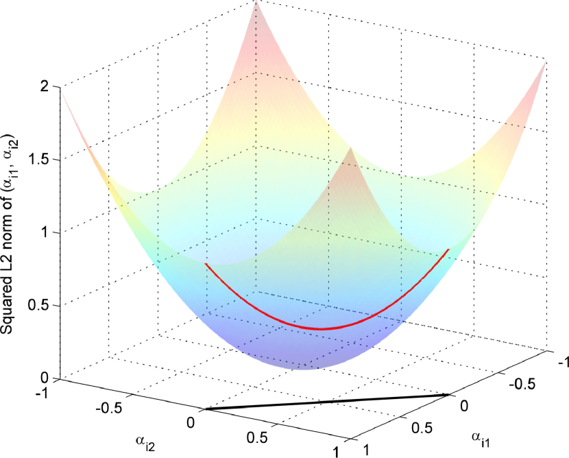
Figure 3: The sparsity promoting effect of maximizing $\|\boldsymbol{\alpha}_{i}\|^{2}$ subject to the simplex constraint when $M=2$. The black line segment in the plane $z=0$ is the simplex constraint. The red line on the paraboloid is the projected values of $\|\boldsymbol{\alpha}_{i}\|^{2}$ from the simplex. Maximizing $\|\boldsymbol{\alpha}_{i}\|^{2}$ will lead to solutions corresponding to the extreme ends of the simplex (sparse solution).

The parameters $\mathbf{r}_{j}$ can also be assumed to be drawn from suitable prior distributions. From the analysis of Figure 1 to obtain a unique solution, we assume that the endmembers should tightly surround the mixed pixels. From the characteristics of function representation, they should also be smooth. So we introduce two types of proximity to model the density function of $\mathbf{R}$. The first makes every two endmembers close to each other, which is also used in [4, 27]. The second makes the adjacent wavelengths have similar values for each endmember. This can be done by using a density function on $\mathbf{R}$ as

$$p(\mathbf{R}) \propto \exp\left\{-\frac{\rho_{1}}{4}\sum_{i=1}^{M}\sum_{j=1}^{M}u_{ij}\|\mathbf{r}_{i}-\mathbf{r}_{j}\|^{2}\right\}\times$$ (11)

$$\text{exp}\left\{-\frac{\rho_{2}}{4}\sum_{k=1}^{B}\sum_{l=1}^{B}v_{kl}\|\mathbf{r}^{k}-\mathbf{r}^{l}\|^{2}\right\}$$

where $\mathbf{r}^{k}$ denotes the $k$th column of $\mathbf{R}$. $u_{ij}=1$ for all $i$ and $j$ so the first term fulfills the first sense of proximity. $v_{kl}$ is 1 when $|k-l|=1$ and 0 otherwise so it actually numerically minimizes $\sum_{j}\int\left(f_{j}^{\prime}(\lambda)\right)^{2}d\lambda$ and satisfies the second proximity. Similar to (10), (11) can be written as

$$p(\mathbf{R})\propto\text{exp}\left\{-\frac{\rho_{1}}{2}\text{Tr}\left(\mathbf{R}^{T}\mathbf{H}\mathbf{R}\right)-\frac{\rho_{2}}{2}\text{Tr}\left(\mathbf{R}\mathbf{G}\mathbf{R}^{T}\right)\right\},$$ (12)

where $\mathbf{H}\in\mathbb{R}^{M\times M}$ and $\mathbf{G}\in\mathbb{R}^{B\times B}$ are the corresponding Laplacian matrices ($\mathbf{H}$ has -1 everywhere except for diagonals with value $M-1$, $\mathbf{G}$ has almost every diagonal element as 2, except for 1 in $v_{11}$ and $v_{BB}$, and -1 in the adjacent diagonals).

2.3 Maximizing the posterior

From the prior probability density in (10), (12) and the conditional probability density in (7), we invoke Bayes’ theorem to get the posterior probability density with a view toward maximizing the posterior. Standard algebra yields

$$p(\mathbf{R},\boldsymbol{\Theta},\mathbf{A},\mu|\mathbf{Y})\propto p(\mathbf{A})p(\mathbf{R})p(\mathbf{Y}|\mathbf{R},\boldsymbol{\Theta},\mathbf{A},\mu)$$

where $p(\boldsymbol{\Theta})$, $p(\mu)$ and $p(\mathbf{Y})$ are assumed to follow a uniform distribution. Maximizing $\log p\left(\mathbf{R},\boldsymbol{\Theta},\mathbf{A},\mu|\mathbf{Y}\right)$ is equivalent to minimizing

$$\mathcal{E}\left(\mathbf{R},\boldsymbol{\Theta},\mathbf{A},\mu\right)= \text{vec}\left((\mathbf{Y}-\mathbf{AR})^{T}\right)^{T}\boldsymbol{\Sigma}_{\mathbf{Y}}^{-1}\text{vec}\left((\mathbf{Y}-\mathbf{AR})^{T}\right)+\log|\boldsymbol{\Sigma}_{\mathbf{Y}}|$$

$$+\beta_{1}\text{Tr}\left(\mathbf{A}^{T}\mathbf{K}\mathbf{A}\right)+\rho_{1}\text{Tr}\left(\mathbf{R}^{T}\mathbf{H}\mathbf{R}\right)+\rho_{2}\text{Tr}\left(\mathbf{R}\mathbf{G}\mathbf{R}^{T}\right)$$ (13)

where $\boldsymbol{\Sigma}_{\mathbf{Y}}$ is given in (8). Notice that the first term in (13) involves inversion of a large non-sparse $NB$ by $NB$ matrix, which is computationally expensive. We now describe methods to reduce the complexity.

Using the Woodbury identity, $\boldsymbol{\Sigma}_{\mathbf{Y}}^{-1}$ becomes

$$\boldsymbol{\Sigma}_{\mathbf{Y}}^{-1} = \left(\mu^{2}\mathbf{I}_{NB}+(\mathbf{A}\otimes\mathbf{I}_{B})[\delta_{ij}\boldsymbol{\Sigma}_{j}](\mathbf{A}\otimes\mathbf{I}_{B})^{T}\right)^{-1}$$ (14)

$$= \mu^{-2}\mathbf{I}_{NB}-\mu^{-2}\left(\mathbf{A}\otimes\mathbf{I}_{B}\right)\mathbf{Q}^{-1}\left(\mathbf{A}\otimes\mathbf{I}_{B}\right)^{T}$$

where

$$\mathbf{Q} = \mu^{2}\left[\delta_{ij}\boldsymbol{\Sigma}_{j}\right]^{-1}+\left(\mathbf{A}\otimes\mathbf{I}_{B}\right)^{T}\left(\mathbf{A}\otimes\mathbf{I}_{B}\right)$$ (15)

$$= \mu^{2}\left[\delta_{ij}\boldsymbol{\Sigma}_{j}^{-1}\right]+\left(\mathbf{A}^{T}\otimes\mathbf{I}_{B}\right)\left(\mathbf{A}\otimes\mathbf{I}_{B}\right)$$

$$= \left[\delta_{ij}\mathbf{S}_{j}\right]+\mathbf{A}^{T}\mathbf{A}\otimes\mathbf{I}_{B}$$

with $\mathbf{S}_{j}=\mu^{2}\boldsymbol{\Sigma}_{j}^{-1}$. Note that $\mathbf{A}^{T}\mathbf{A}\otimes\mathbf{I}_{B}$ is a positive semidefinite matrix and therefore $\mathbf{Q}\in\text{SPD}\left(MB\right)$ ($\boldsymbol{\Sigma}_{j}\in\text{SPD}\left(B\right)$). Plugging (14) into the first term of the objective function leads to

$$\text{vec}\left((\mathbf{Y}-\mathbf{AR})^{T}\right)^{T}\boldsymbol{\Sigma}_{\mathbf{Y}}^{-1}\text{vec}\left((\mathbf{Y}-\mathbf{AR})^{T}\right)$$ (16)

$$= \mu^{-2}\|\mathbf{Y}-\mathbf{A}\mathbf{R}\|_{F}^{2}-\mu^{-2}\mathbf{z}^{T}\mathbf{Q}^{-1}\mathbf{z},$$

where

$$\mathbf{z} = \left(\mathbf{A}\otimes\mathbf{I}_{B}\right)^{T}\text{vec}\left(\left(\mathbf{Y}-\mathbf{A}\mathbf{R}\right)^{T}\right)$$

$$= \left(\mathbf{A}^{T}\otimes\mathbf{I}_{B}\right)\text{vec}\left(\left(\mathbf{Y}-\mathbf{A}\mathbf{R}\right)^{T}\right)$$

$$= \text{vec}\left(\left(\mathbf{Y}-\mathbf{A}\mathbf{R}\right)^{T}\mathbf{A}\right).$$

From Sylvester’s determinant theorem, the logarithm term $\text{log}\left|\boldsymbol{\Sigma}_{\mathbf{Y}}\right|$ becomes

$$\text{log}\left|\mu^{2}\mathbf{I}_{NB}+\left(\mathbf{A}\otimes\mathbf{I}_{B}\right)\left[\delta_{ij}\boldsymbol{\Sigma}_{j}\right]\left(\mathbf{A}\otimes\mathbf{I}_{B}\right)^{T}\right|$$ (17)

$$= \text{log}\mu^{2NB}\left|\mathbf{I}_{MB}+\mu^{-2}\left[\delta_{ij}\boldsymbol{\Sigma}_{j}\right]\left(\mathbf{A}\otimes\mathbf{I}_{B}\right)^{T}\left(\mathbf{A}\otimes\mathbf{I}_{B}\right)\right|$$

$$= \text{log}\mu^{2NB}\left|\mu^{-2}\left[\delta_{ij}\boldsymbol{\Sigma}_{j}\right]\right|\left|\mu^{2}\left[\delta_{ij}\boldsymbol{\Sigma}_{j}\right]^{-1}+\mathbf{A}^{T}\mathbf{A}\otimes\mathbf{I}_{B}\right|$$

$$= NB\text{log}\mu^{2}-\text{log}\left|\left[\delta_{ij}\mathbf{S}_{j}\right]\right|+\text{log}\left|\mathbf{Q}\right|.$$

Combining the results in (16) and (17), and letting $\gamma=\mu^{-2}$, minimizing (13) becomes equivalent to minimizing $\mathcal{E}_{1}\left(\mathbf{R},\mathbf{A},\gamma,\left\{\mathbf{S}_{j}\right\}\right)$ as

$$\mathcal{E}_{1}(\mathbf{R},\mathbf{A},\gamma,\left\{\mathbf{S}_{j}\right\}) = \gamma\|\mathbf{Y}-\mathbf{A}\mathbf{R}\|_{F}^{2}-\gamma\mathbf{z}^{T}\mathbf{Q}^{-1}\mathbf{z}+\text{log}\left|\mathbf{Q}\right|$$ (18)

$$-\sum_{j=1}^{M}\text{log}\left|\mathbf{S}_{j}\right|-NB\text{log}\gamma+\beta_{1}\text{Tr}\left(\mathbf{A}^{T}\mathbf{K}\mathbf{A}\right)$$

$$+\rho_{1}\text{Tr}\left(\mathbf{R}^{T}\mathbf{H}\mathbf{R}\right)+\rho_{2}\text{Tr}\left(\mathbf{R}\mathbf{G}\mathbf{R}^{T}\right)$$

subject to

$$\mathbf{A}\geq 0,\,\mathbf{A}\mathbf{1}_{M}=\mathbf{1}_{N},\,\mathbf{R}\geq 0,\,\mathbf{S}_{j}\in\text{SPD}\left(B\right)$$ (19)

where $\mathbf{Q}=\left[\delta_{ij}\mathbf{S}_{j}\right]+\mathbf{A}^{T}\mathbf{A}\otimes\mathbf{I}_{B}$, $\mathbf{z}=\text{vec}\left(\left(\mathbf{Y}-\mathbf{A}\mathbf{R}\right)^{T}\mathbf{A}\right)$. Note that letting $\boldsymbol{\Sigma}_{j}\rightarrow\mathbf{0}$ (i.e. there is little endmember uncertainty) will result in $\mathbf{S}_{j}$ tending to infinity and $\gamma\mathbf{z}^{T}\mathbf{Q}^{-1}\mathbf{z}$ vanishing, resulting in $\text{log}\left|\mathbf{Q}\right|$ canceling $\sum_{j=1}^{M}\text{log}\left|\mathbf{S}_{j}\right|$ as $\left[\delta_{ij}\mathbf{S}_{j}\right]$ dominates $\mathbf{Q}$. Thus the entire objective function reduces to the widely used least squares objective.

2.4 Optimizing the objective function

The objective function (18) is not convex. Given an initial condition, we can use the block coordinate descent method to find a suitable local minimum (please Section 2.7 in [5]). That is, for $n=0,1,2,...$, $\mathbf{A},\,\mathbf{R}$ and $\gamma,\,\left\{\mathbf{S}_{j}\right\}$ are alternately updated by

$$\mathbf{A}^{n+1},\,\mathbf{R}^{n+1}=\arg\min_{\mathbf{R},\mathbf{A}}\mathcal{E}_{1}\left(\mathbf{R},\mathbf{A},\gamma^{n},\left\{\mathbf{S}_{j}^{n}\right\}\right),$$

$$\gamma^{n+1},\,\left\{\mathbf{S}_{j}^{n+1}\right\}=\arg\min_{\gamma,\left\{\mathbf{S}_{j}\right\}}\mathcal{E}_{1}\left(\mathbf{R}^{n+1},\mathbf{A}^{n+1},\gamma,\left\{\mathbf{S}_{j}\right\}\right),$$

subject to the constraints (19). We show in the Appendix that $\gamma\mathbf{z}^{T}\mathbf{Q}^{-1}\mathbf{z}$ and $\text{log}\left|\mathbf{Q}\right|-\sum_{j=1}^{M}\text{log}\left|\mathbf{S}_{j}\right|$ are positive and are small compared to $\gamma\|\mathbf{Y}-\mathbf{A}\mathbf{R}\|_{F}^{2}$ (also verified in the experiments to follow). Hence, when minimizing $\mathcal{E}_{1}$ with respect to $\mathbf{A}$ and $\mathbf{R}$, we can ignore these terms and instead minimize $\mathcal{E}_{2}\left(\mathbf{R},\mathbf{A}\right)$:

$$\mathcal{E}_{2} = \|\mathbf{Y}-\mathbf{A}\mathbf{R}\|_{F}^{2}+\frac{\beta_{1}}{\gamma}\text{Tr}\left(\mathbf{A}^{T}\mathbf{K}\mathbf{A}\right)$$ (20)

$$+\frac{\rho_{1}}{\gamma}\text{Tr}\left(\mathbf{R}^{T}\mathbf{H}\mathbf{R}\right)+\frac{\rho_{2}}{\gamma}\text{Tr}\left(\mathbf{R}\mathbf{G}\mathbf{R}^{T}\right).$$

Also, in this case, $\gamma$ will not impact the solution of $\mathbf{A}$ and $\mathbf{R}$ because the ratio of parameters, e.g. $\beta_{1}/\gamma$, will become the new parameters to tune. Assume when optimizing with respect to $\mathbf{A},\,\mathbf{R}$, $\gamma$ is the optimal value. The subsequent optimization with respect to $\gamma,\,\left\{\mathbf{S}_{j}\right\}$ will not change the next iteration result of $\mathbf{A},\,\mathbf{R}$, which in turn keeps $\gamma,\,\left\{\mathbf{S}_{j}\right\}$ unchanged. So the block coordinate descent becomes a simple two step algorithm where the first step minimizes (20) with respect to $\mathbf{A},\,\mathbf{R}$ and the second step minimizes (18) with respect to $\gamma,\,\left\{\mathbf{S}_{j}\right\}$ given the obtained $\mathbf{A},\,\mathbf{R}$. Note that again both of them are optimizations over convex sets ($\mathbf{A}$ is restricted to the Cartesian product of simplices, $\mathbf{S}_{j}$ is restricted to the convex cone of positive definite matrices) and so gradient projection methods can be used to solve these kind of problems (please see Section 2.3 in [5]).

Though the objective function (20) is not convex, it is convex with respect to either $\mathbf{A}$ or $\mathbf{R}$ (e.g. it can be written as a quadratic function with respect to $\mathbf{A}$: $\frac{1}{2}\mathbf{x}^{T}\mathbf{Q}\mathbf{x}+\mathbf{b}^{T}\mathbf{x}$ where $\mathbf{x}=\text{vec}\left(\mathbf{A}\right)$, $\mathbf{Q}=\mathbf{R}\mathbf{R}^{T}\otimes\mathbf{I}_{N}+\frac{\beta_{1}}{\gamma}\mathbf{I}_{M}\otimes\mathbf{K}$, $\mathbf{b}=-\text{vec}\left(\mathbf{Y}\mathbf{R}^{T}\right)$). We can alternately update $\mathbf{A}$ and $\mathbf{R}$ to reduce the energy. Taking derivatives of (20) with respect to $\mathbf{A}$, we have

$$\frac{\partial\mathcal{E}_{2}}{\partial\mathbf{A}}=2\left(-\mathbf{Y}\mathbf{R}^{T}+\mathbf{A}\mathbf{R}\mathbf{R}^{T}+\frac{\beta_{1}}{\gamma}\mathbf{KA}\right).$$ (21)

The gradient projection method sets the value of the next iteration, $\mathbf{A}^{n+1}$, to be the projected value of the steepest descent

$$\mathbf{A}^{n+1}=\phi\left(\mathbf{A}^{n}-\frac{\tau^{n}}{2}\frac{\partial\mathcal{E}_{2}}{\partial\mathbf{A}}\left(\mathbf{R}^{n},\mathbf{A}^{n}\right)\right),$$ (22)

where

$$\phi:\,\mathbf{X}\mapsto\arg\min_{\mathbf{Y}\in\mathbb{R}^{N\times M}}\|\mathbf{X}-\mathbf{Y}\|_{F}^{2}\,\text{s.t. }\mathbf{Y}\geq 0,\,\mathbf{Y}\mathbf{1}_{M}=\mathbf{1}_{N}$$

projects a matrix to the nearest matrix that satisfies the simplex constraint (e.g. we use the algorithm of Figure 1 in [8]). $\tau^{n}>0$ is the step size and is set by 1D minimization or the familiar Armijo rule. It is shown that the sequence generated by (22) is gradient related, i.e. $\left\langle\frac{\partial\mathcal{E}_{2}}{\partial\mathbf{A}}\left(\mathbf{R}^{n},\mathbf{A}^{n}\right),\mathbf{A}^{n+1}-\mathbf{A}^{n}\right\rangle<0$ (Proposition 2.3.1 in [5]), which leads to a stationary point given proper step sizes $\tau^{n}$ such as the exact line minimization of [14],

$$\tau^{n}=\arg\min_{\tau\geq 0}\mathcal{E}_{2}\left(\mathbf{R}^{n},\phi\left(\mathbf{A}^{n}-\frac{\tau}{2}\frac{\partial\mathcal{E}_{2}}{\partial\mathbf{A}}\left(\mathbf{R}^{n},\mathbf{A}^{n}\right)\right)\right).$$

Numerically, we can use adaptive step sizes that start with a small step and gradually increase it by an order of magnitude until $\mathcal{E}_{2}$ starts increasing. Similar gradient descent methods were proposed in [13, 19], and it is shown that such methods have a faster convergence rate than those based on multiplicative update rules [7, 20].

Once we have updated $\mathbf{A}$, we can update $\mathbf{R}$ by finding a new value that reduces (20). A gradient projection method can also be used for $\mathbf{R}$ because of the positivity constraint. However, the introduction of spatial smoothness and the sparsity promoting term, $\text{Tr}\left(\mathbf{A}^{T}\mathbf{K}\mathbf{A}\right)$, along with the pairwise closeness term actually make $\mathbf{R}$ seldom negative even when just using a closed form solution. Taking derivatives of (20) with respect to $\mathbf{R}$, we have

$$\frac{\partial\mathcal{E}_{2}}{\partial\mathbf{R}}=2\left(\mathbf{A}^{T}\mathbf{A}\mathbf{R}-\mathbf{A}^{T}\mathbf{Y}+\frac{\rho_{1}}{\gamma}\mathbf{HR}+\frac{\rho_{2}}{\gamma}\mathbf{RG}\right).$$

Letting $\frac{\partial\mathcal{E}_{2}}{\partial\mathbf{R}}=0$, we obtain a closed form solution for $\mathbf{R}$ that ignores the positivity constraint,

$$\left(\mathbf{A}^{T}\mathbf{A}+\frac{\rho_{1}}{\gamma}\mathbf{H}\right)\mathbf{R}+\frac{\rho_{2}}{\gamma}\mathbf{RG}=\mathbf{A}^{T}\mathbf{Y}.$$ (23)

Equation (23) is called a Sylvester equation in control theory which is normally solved by performing a Schur decomposition of the two matrices before and after $\mathbf{R}$ and back substitution of the resulting equations [3]. Given an initial condition, we can alternately update $\mathbf{A}$ and $\mathbf{R}$ based on (22) and (23). The details are given in the first two steps in Algorithm 1. Since at each step the energy is lowered, the algorithm will lead to a local minimum.

Given the estimated endmembers and abundances, we can find $\gamma,\,\left\{\mathbf{S}_{j}\right\}$ (hence $\mu$ and $\boldsymbol{\Sigma}_{j}$) similarly. Taking derivatives of (18) with respect to $\gamma$ and setting it to zero, we have

$$\gamma^{-1}=\frac{1}{NB}\left\{\|\mathbf{Y}-\mathbf{A}\mathbf{R}\|_{F}^{2}-\mathbf{z}^{T}\mathbf{Q}^{-1}\mathbf{z}\right\}.$$ (24)

Note that the right hand side of (24) is always greater than 0 from (16). Using the chain rule in matrix form to take derivatives of (18) with respect to $\mathbf{S}_{j}$, we have

$$\frac{\partial\mathcal{E}_{1}}{\partial\mathbf{S}_{j}}=\left(\gamma\mathbf{Q}^{-1}\mathbf{z}\mathbf{z}^{T}\mathbf{Q}^{-1}\right)_{j}-\mathbf{S}_{j}^{-1}+\left(\mathbf{Q}^{-1}\right)_{j},$$ (25)

where $\left(\cdot\right)_{j}$ denotes the extraction of the $j$th diagonal $B$ by $B$ block of the $MB$ by $MB$ matrix. Hence, we can alternately update $\gamma$ and $\mathbf{S}_{j}$ to minimize (18) keeping $\mathbf{A},\,\mathbf{R}$ fixed. For updating $\mathbf{S}_{j}$, a similar gradient projection method as (22) can be used, where the projection onto the set of positive definite matrices is obtained by truncating the eigenvalues[1]. The details are given in Step 3 of Algorithm 1.

Algorithm 1 The implementation of SCM

Input: $\mathbf{Y}=\left[\mathbf{y}_{1},...,\mathbf{y}_{N}\right]^{T}$, $M$, $\eta$, $\beta_{1}^{\prime}$, $\beta_{2}^{\prime}$, $\rho_{1}^{\prime}$, $\rho_{2}^{\prime}$, $\sigma_{0}$, $\sigma_{\text{max}}$.

• Step 1: Initialize $\frac{\beta_{1}}{\gamma}=\frac{B}{M}\beta_{1}^{\prime}$, $\frac{\beta_{2}}{\gamma}=\frac{B}{M}\beta_{2}^{\prime}$, $\frac{\rho_{1}}{\gamma}=\frac{N}{M^{2}}\rho_{1}^{\prime}$, $\frac{\rho_{2}}{\gamma}=\frac{N}{M}\rho_{2}^{\prime}$¹. Construct the Laplacian matrices $\mathbf{L}$, $\mathbf{H}$ and $\mathbf{G}$.

• Step 2: Initialize $\mathbf{R}$ to be the centers of $M$ clusters of $\mathbf{Y}$ by K-means². Initialize $\mathbf{A}=\phi\left(\mathbf{Y}\mathbf{R}^{T}\left(\mathbf{R}\mathbf{R}^{T}+\epsilon\mathbf{I}_{M}\right)^{-1}\right)$, where $\phi\left(\mathbf{A}\right):\mathbf{A}\mapsto\left[\max\left(\alpha_{ij}-\theta_{i},0\right)\right]$ where $\theta_{i}=\frac{1}{K_{i}}\left(\sum_{k=1}^{K_{i}}\alpha_{ik}^{\prime}-1\right)$, $\alpha_{i1}^{\prime}\geq...\geq\alpha_{iM}^{\prime}$ are sorted $\alpha_{i1},...,\alpha_{iM}$, $K_{i}$ is the largest $k$ such that $\alpha_{ik}^{\prime}-\frac{1}{k}\left(\sum_{l=1}^{k}\alpha_{il}^{\prime}-1\right)>0$. Solve $\mathbf{A},\,\mathbf{R}$ by repeating the following two steps until convergence.

  • Update $\mathbf{A}$ by $\phi_{A}\left(\tau\right)=\phi\left(\mathbf{A}-\frac{\tau}{2}\frac{\partial\mathcal{E}_{2}}{\partial\mathbf{A}}\right)$, where $\frac{\partial\mathcal{E}_{2}}{\partial\mathbf{A}}$ is given in (21). If $\mathcal{E}_{2}\left(\mathbf{R},\phi_{A}\left(\tau_{\epsilon}\right)\right)<\mathcal{E}_{2}\left(\mathbf{R},\mathbf{A}\right)$, $\tau$ attempts $\tau_{\epsilon}10^{i}$, $i=0,1,2,...$ until $\mathcal{E}_{2}\left(\mathbf{R},\phi_{A}\left(\tau_{\epsilon}10^{i+1}\right)\right)\geq\mathcal{E}_{2}\left(\mathbf{R},\phi_{A}\left(\tau_{\epsilon}10^{i}\right)\right)$, otherwise set $\tau=0$.

  • Update $\mathbf{R}$ by solving (23)³.

• Step 3: Initialize $\gamma^{-1}=\frac{1}{NB}\|\mathbf{Y}-\mathbf{A}\mathbf{R}\|_{F}^{2}$, $\boldsymbol{\Sigma}_{j}=\sigma_{0}^{2}\mathbf{I}_{B}$. Define $\psi\left(\mathbf{X}\right):\mathbf{X}\mapsto\mathbf{U}\left[\delta_{ij}\text{max}\left(\lambda_{i},1/\gamma\sigma_{\text{max}}^{2}\right)\right]\mathbf{U}^{T}$ where $\mathbf{X}=\mathbf{U}\left[\delta_{ij}\lambda_{i}\right]\mathbf{U}^{T}$ is the eigendecomposition. Solve $\gamma,\,\left\{\mathbf{S}_{j}\right\}$ by repeating the following two steps until convergence.

  • Update $\mathbf{S}_{j}$ by $\psi_{j}\left(\tau\right)=\psi\left(\mathbf{S}_{j}-\tau\frac{\partial\mathcal{E}_{1}}{\partial\mathbf{S}_{j}}\right)$ for $j=1,...,M$, where $\frac{\partial\mathcal{E}_{1}}{\partial\mathbf{S}_{j}}$ is given in (25). The step size $\tau$ is determined similar to step 2.

  • Update $\gamma$ by (24).

Output: $\mathbf{A}$, $\mathbf{R}$, $\mu=\gamma^{-1/2}$, $\boldsymbol{\Sigma}_{j}=\mu^{2}\mathbf{S}_{j}^{-1}$.

Remark 1. The choice of free parameters should be invariant with respect to the changing magnitude of each term in (20) with different $N$, $M$ and $B$. For example, the first term in (20) has a magnitude of $NB$. From the banded diagonal nature of $\left[w_{ij}\right]$ in (10), $\text{Tr}\left(\mathbf{A}^{T}\mathbf{L}\mathbf{A}\right)$ has a magnitude of $NM$. So the parameter $\beta_{1}$ should have a magnitude of $\beta_{1}/\gamma=\beta_{1}^{\prime}B/M$. Similarly, the parameters $\beta_{2}$, $\rho_{1}$ and $\rho_{2}$ should have magnitudes according to $\beta_{2}/\gamma=\beta_{2}^{\prime}B/M$, $\rho_{1}/\gamma=\rho_{1}^{\prime}N/M^{2}$, $\rho_{2}/\gamma=\rho_{2}^{\prime}N/M$.

Remark 2. The initial endmembers are important in endmember estimation. Randomly picking pixels and fast algorithms such as VCA can provide an initial estimate. We find that K-means works well in practical applications. This could be due to the fact that K-means can pre-segment the image to obtain the mean values of different regions.

Remark 3. We can resort to the classical Krylov subspace method to solve the transposed version of (23) more efficiently [12]. That is, for $\mathbf{A}\mathbf{X}+\mathbf{X}\mathbf{B}=\mathbf{C}$ where $\mathbf{A}\in\mathbb{R}^{B\times B}$, $\mathbf{B}\in\mathbb{R}^{M\times M}$, $\mathbf{X},\,\mathbf{C}\in\mathbb{R}^{B\times M}$, $B\gg M$, $\mathbf{A}$ is sparse and $\mathbf{B}$ is symmetric, the eigendecomposition $\mathbf{B}=\mathbf{U}\boldsymbol{\Lambda}\mathbf{U}^{T}$ ($\boldsymbol{\Lambda}=\left[\delta_{ij}\lambda_{i}\right]$ consists of eigenvalues) shows that it is equivalent to $\mathbf{A}\mathbf{Y}+\mathbf{Y}\boldsymbol{\Lambda}=\mathbf{D}$ where $\mathbf{Y}=\mathbf{X}\mathbf{U}$, $\mathbf{D}=\mathbf{C}\mathbf{U}$. Let $\mathbf{Y}=\left[\mathbf{y}_{1},...,\mathbf{y}_{M}\right]$, $\mathbf{D}=\left[\mathbf{d}_{1},...,\mathbf{d}_{M}\right]$, we have a linear system of equations $\left(\mathbf{A}+\lambda_{i}\mathbf{I}\right)\mathbf{y}_{i}=\mathbf{d}_{i}$ for each column, where $\mathbf{y}_{i}$ can be solved independently and efficiently since $\mathbf{A}$ is sparse. Then, $\mathbf{X}$ can be recovered using $\mathbf{X}=\mathbf{Y}\mathbf{U}^{T}$.

3 Results

In the experiments, all the algorithms were implemented in MATLAB^®. For endmember extraction, we compared the SCM algorithm with NCM and PCOMMEND [27], where NCM was implemented as SCM with $\beta_{1}^{\prime}=0$, $\beta_{2}^{\prime}=0$, $\rho_{2}^{\prime}=0$. The parameters of SCM have fixed $\eta=0.05$, $\beta_{1}^{\prime}=0.01$, $\rho_{2}^{\prime}=0$, $\sigma_{0}=0.1$, $\sigma_{\text{max}}=1$ for all the cases. The parameters of PCOMMEND were tuned to give the best result in each case. Throughout the experiments, we use the mean of absolute difference as the error, i.e., $\frac{1}{NM}\sum_{i,j}|\alpha_{ij}-\alpha_{ij}^{\prime}|$ for error of abundances, $\frac{1}{MB}\sum_{i,j}|m_{ij}-m_{ij}^{\prime}|$ for error of endmembers. Because the endmembers from algorithms may have a different permutation from the ground truth endmembers, we permuted the results from algorithms to calculate the error.

For measuring and visualizing the uncertainty from $\left\{\boldsymbol{\Sigma}_{j}\right\}$, recall that the covariance matrix of a Gaussian distribution determines the shape of the distribution, i.e. the eigenvectors are the directions of the variation patterns while the eigenvalues are the variances of the projected (onto the eigenvectors) 1D data points. The uncertainty can be measured by the largest eigenvalue and its corresponding eigenvector. We use the square root of the largest eigenvalue, $\sigma$, as the uncertainty amount since it corresponds to the standard deviation. Then, the corresponding eigenvector (normalized), $\mathbf{u}$, can be viewed as the uncertainty direction. The uncertainty range can be visualized by the estimated endmember $\mathbf{r}$ plus (minus) twice the uncertainty direction with uncertainty amount, i.e. $\mathbf{r}\pm 2\sigma\mathbf{u}$.

3.1 Synthetic images

We first test SCM on synthetic images generated from the true material spectra in the Aster spectral library [2]. We picked 2 rocks (limestone, basalt), 2 man-made materials (concrete, asphalt) in the experiments. The spectra of these endmembers are shown in Figure 4. The wavelength of these materials ranges from 0.4$\mu$m to 14$\mu$m. For each material, the reflectance of this range is re-sampled into 200 values.

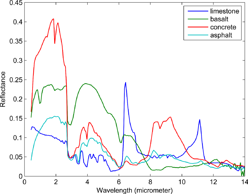
Figure 4: Spectral signatures of the 4 endmembers used to generate synthetic images.

A set of synthetic images of size 40 by 40 were generated using the 4 endmembers with different noise levels. For each image, the domain is divided into 4 rectangular regions, where each region contains a pure material. Hence, the abundance maps contain 1 corresponding to the pure material at each pixel and 0 for the other materials. Then, each abundance map is convolved with an isotropic 2D Gaussian filter such that the boundary between regions is blurred and the nearby pixels contain mixed materials. At the end, an additive noise with mean zero and standard deviation $\sigma_{Y}$ is added to the image. We conducted experiments on these images to verify the ability to find endmembers and the ability to estimate the uncertainty.

For endmember extraction, we compared SCM, NCM, and PCOMMEND based on 5 levels of signal-to-noise ratio (SNR), from 20dB ($\sigma_{Y}\approx 0.01$) to 60dB ($\sigma_{Y}\approx 0.0001$). 20 random images were generated in each case such that the average error can be calculated. The parameters of SCM were $\beta_{2}^{\prime}=0$, $\rho_{1}^{\prime}=0.005$. Figure 5 shows the errors of all the algorithms. From the plots, we can see that SCM has lower errors than NCM and PCOMMEND for all the noise cases, with respect to both endmembers and abundances. Figure 6 shows the abundance maps from these algorithms for a noisy synthetic image. We can see that the abundance maps of NCM and PCOMMEND present more fuzzy abundances within a pure material region due to the noise. Meanwhile, SCM presents consistent abundances within such a region.

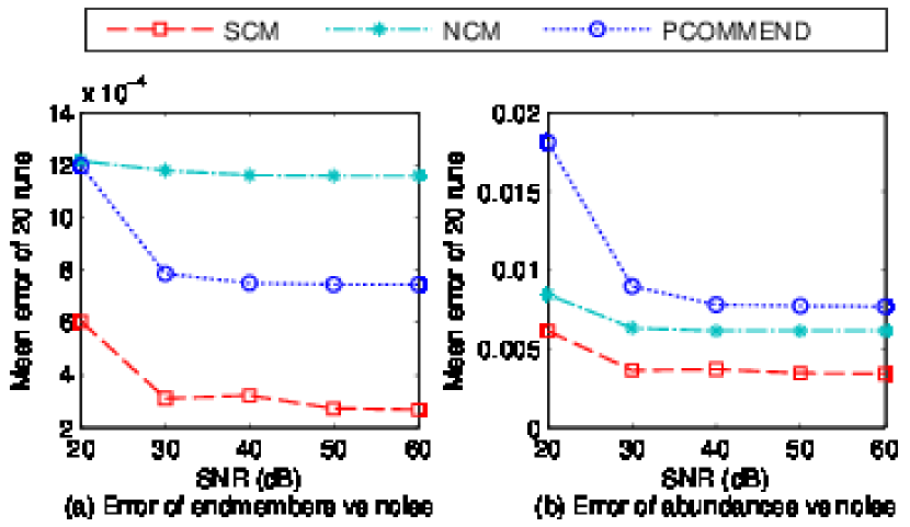
Figure 5: Error of endmembers and abundances based on the synthetic imagesfor all the algorithms.

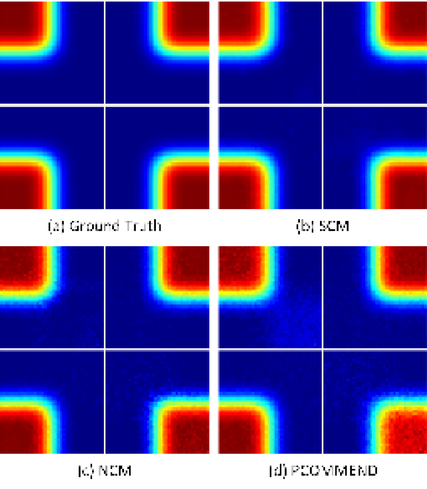
Figure 6: Abundance maps from the ground truth (a), SCM (b), NCM (c) and PCOMMEND (d) for a noisy synthetic image with SNR 20dB.

For uncertainty estimation, we compared the uncertainties based on different estimated endmembers for the same material in a synthetic image with SNR 40dB. To achieve this, we changed the value of $\rho_{1}^{\prime}$ from large to small gradually. This causes the location of the estimated endmembers to change from being close together inside the pixel cloud to sparsely scattered outside the pixel cloud. We pick the uncertainty amount of limestone to represent the whole uncertainty. Figure 7 shows this value along with the error of endmembers versus decreasing $\rho_{1}^{\prime}$. The error of endmembers has its minimum in the middle between $10^{-2}$ and $10^{-3}$. Interestingly, this is also the place where the uncertainty amount starts to decrease to a stable value. This corresponds to the intuition that when the endmembers are outside the pixel cloud, all the pixels can be well represented by the endmembers thus we have a low uncertainty, while when the endmembers are inside the pixel cloud, the more they are closely packed together, more the uncertainty as more pixels are beyond their representation capabilities. Recalling our fundamental question about error prediction, the result here implies that we are capable of estimating the uncertainty.

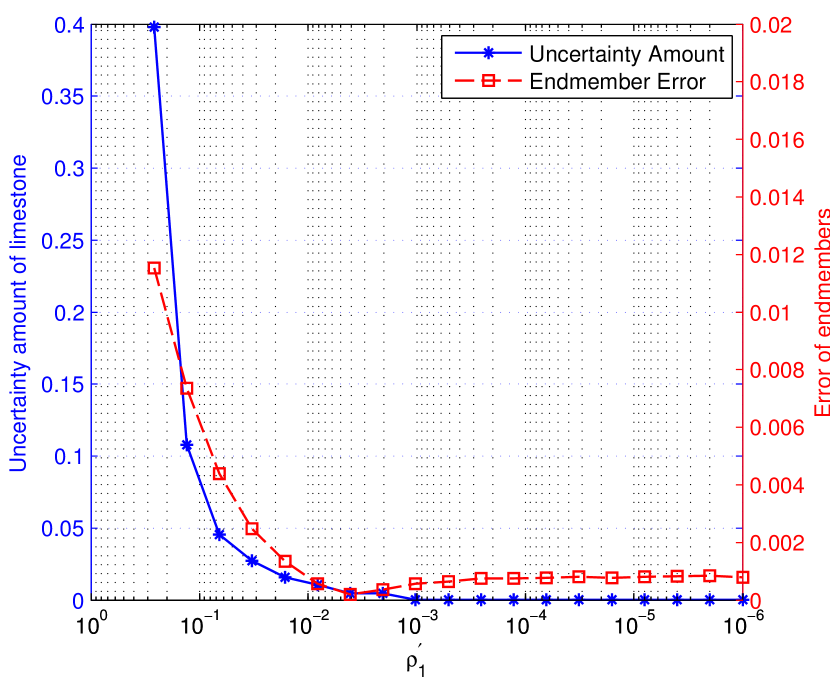
Figure 7: Effect of pairwise closeness ($\rho_{1}^{\prime}$) on the uncertainty amount of limestone (blue solid line, scale on the left) and the error of endmembers (red dashed line, scale on the right) for a synthetic image with SNR 40dB. The minimal error corresponds to the starting point where the uncertainty amount drops to a stable value.

Figure 8 shows the uncertainty range with close endmembers when $\rho_{1}^{\prime}=0.1$. From Figure 7, the endmembers are actually inside the pixel cloud since it is greater than the optimal value. We can see that not only the uncertainty amount reflects the distance to the ground truth, the uncertainty direction also reflects the distortion of the estimated endmembers. Combing these pieces of information, the uncertainty range is able to cover the ground truth for each endmember. Therefore the uncertainty estimated can serve as a prediction of the endmember error in this case, given endmembers estimated with a sufficient closeness constraint.

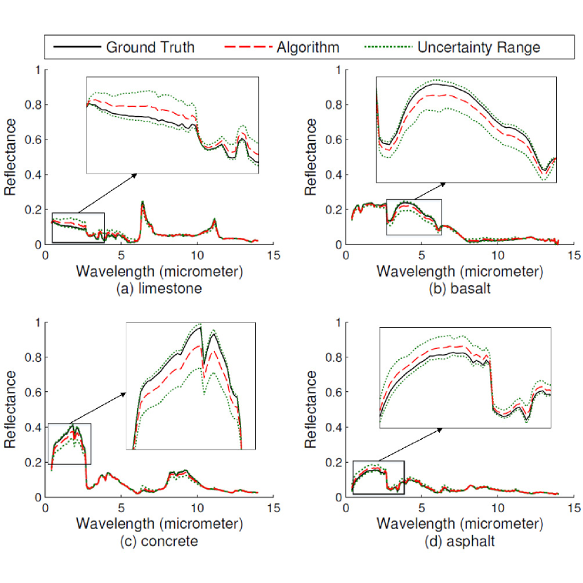
Figure 8: Uncertainty ranges with endmembers estimated with $\rho_{1}^{\prime}=0.1$ for the synthetic image tested in Figure 7. The uncertainty ranges cover the ground truth given endmembers estimated with slight biases.

3.2 Pavia University

The SCM algorithm is also applied to the Pavia University dataset, which was recorded by the Reflective Optics System Imaging Spectrometer (ROSIS) during a flight over Pavia, northern Italy. It is a 340 by 610 image with 103 bands with wavelengths ranging from 430nm to 860nm. The real spacing is 1.3 meters. The image covers both natural and urban areas as shown in Figure 9. There are 9 materials identified as ground truth by humans. From the pixels identified as ground truth, average spectra for each material is calculated as the ground truth endmember signature. Figure 10 shows the ground truth endmembers. From Figure 10, we find that self-blocking bricks and gravel have very similar spectra and asphalt and bitumen have very similar spectra. So technically, in this unsupervised unmixing setting, we can use automated algorithms to distinguish at most 7 endmembers.

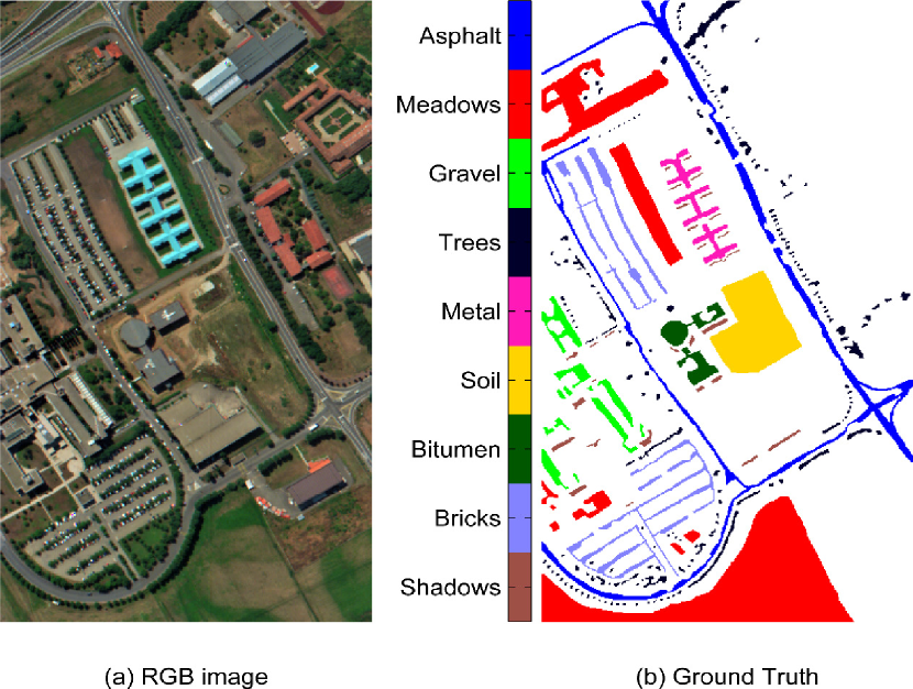
Figure 9: RGB image for Pavia University and the ground truth.

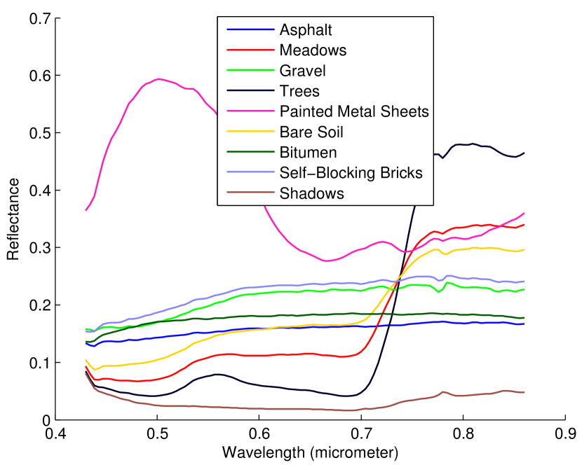
Figure 10: Ground truth endmembers for Pavia University. Asphalt and Bitumen have similar spectral signatures. Gravel and Self-blocking bricks have similar spectral signatures.

We run SCM, NCM, PCOMMEND on this dataset with 7 endmembers (PCOMMEND with 6 endmembers as suggested in [27]). The parameters for SCM are $\beta_{2}^{\prime}=0.02$, $\rho_{1}^{\prime}=0.05$. Two materials, gravel and bitumen, are excluded in the comparison because they are attributed to self-blocking bricks and asphalt respectively. Figure 11(a) shows the abundance maps from SCM. When compared to the ground truth in Figure 9, we can see that the materials are asphalt (bitumen), meadows, trees, painted metal sheets, bare soil, self-blocking bricks (gravel) and shadows respectively. The abundance maps of NCM are shown in Figure 11(b). We observe that without the spatial information and the sparsity promoting effect, the abundance maps present scattered dots within a pure material region.

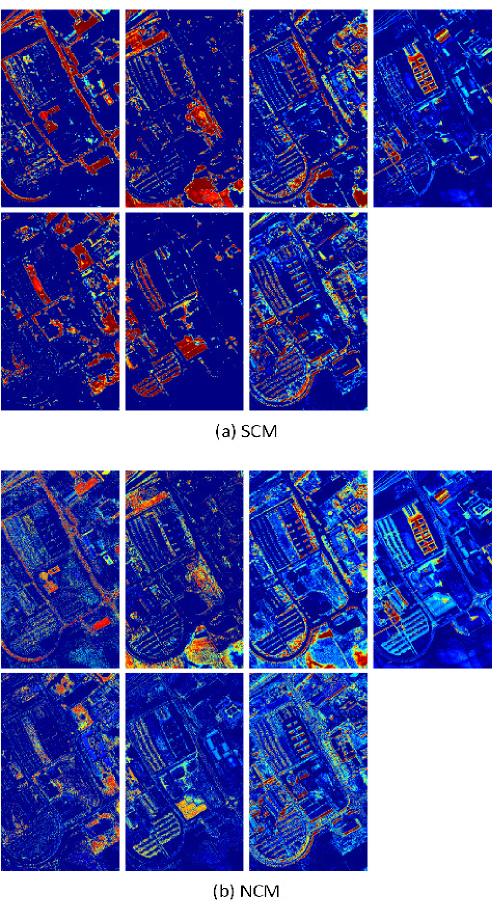
Figure 11: Abundance maps from SCM and NCM for Pavia University. The identified materials are asphalt (bitumen), meadows, trees, painted metal sheets, bare soil, self-blocking bricks (gravel), shadows respectively.

Figure 12 shows the resulting endmember spectra from SCM, NCM, PCOMMEND versus the corresponding ground truth endmember. We also computed the errors for these endmembers and the result is shown in Table 1. From these results, we see that for the 7 identified endmembers, the meadows are missing in PCOMMEND (and this is attributed to wrong ground truth information regarding meadows). Also, SCM matches the asphalt, meadows, trees, bare soil and self-blocking bricks best while NCM matches the painted metal sheets best and PCOMMEND matches the shadows best. The statistics show that SCM performed best overall (except for a caveat that the meadows endmembers should be further investigated due to a discrepancy in the ground-truth).

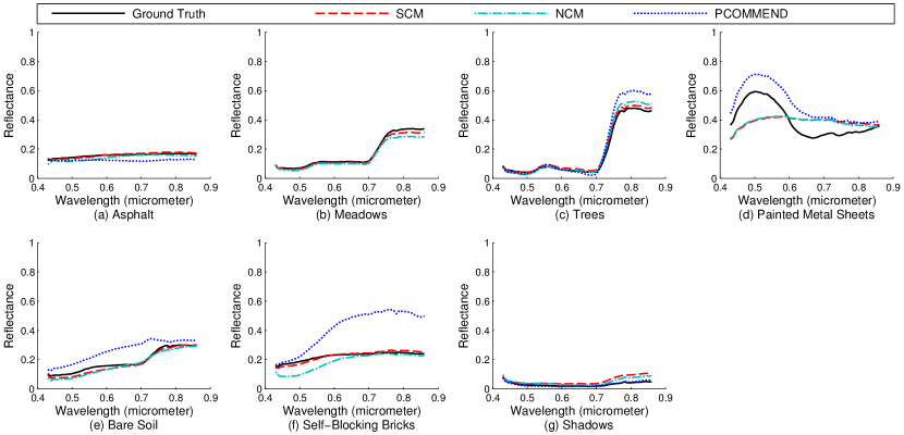
Figure 12: Qualitative comparison of endmembers among all the algorithms for Pavia University.

Table 1: Quantitative comparison of endmembers among all the algorithms for Pavia University.

Error	SCM	NCM	PCOMMEND
Asphalt	0.0064	0.0149	0.0335
Meadows	0.0095	0.0227	-
Trees	0.0135	0.0197	0.0419
Painted Metal Sheets	0.1007	0.0947	0.1096
Bare Soil	0.0144	0.0213	0.0748
Self-Blocking Bricks	0.0105	0.0378	0.1885
Shadows	0.0251	0.0170	0.0043
Average	0.0257	0.0326	0.0754

The uncertainty ranges of endmembers from SCM for Pavia University along with the ground truth are shown in Figure 13. We see that for those well estimated endmembers, the uncertainties are so small that the endmembers coincide with the uncertainty ranges. For the largely biased endmember of painted metal sheets, the uncertainty is also large such that it nearly covers the ground truth. For the shadows, the SCM estimated endmember deviates from the ground truth at the right end and the uncertainty range also features a large gap at the right end.

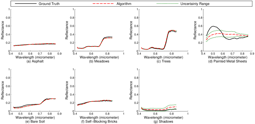
Figure 13: Uncertainty ranges of endmembers estimated from SCM for Pavia University.

3.3 Indian Pines

The Indian Pines dataset was collected by the Airborne Visible/Infrared Imaging Spectrometer (AVIRIS) sensor over the Indian Pines test site in Northwestern Indiana. It is a 145 by 145 image with 220 bands in the wavelength range 0.4 - 2.5$\mu$m. Most areas of the image are agriculture, forest and other vegetation, except two highways, a railway line, and a few buildings. Figure 14 shows the RGB image of this dataset and the ground truth materials. Figure 15 shows the ground truth endmembers. We can see that the ground truth distinguishes the pixels into 16 classes, where most have quite similar spectra.

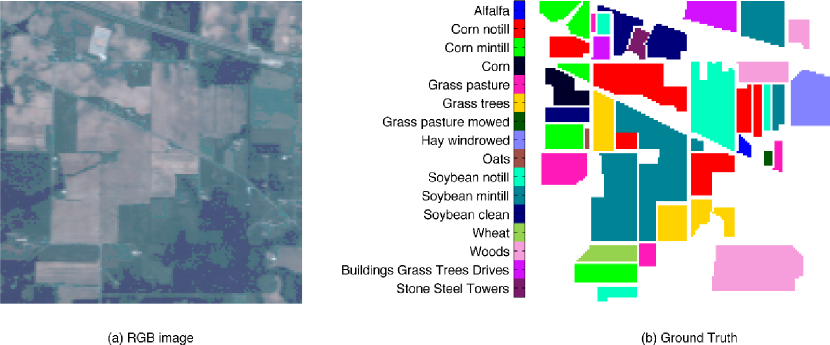
Figure 14: RGB image for Indian Pines and the ground truth.

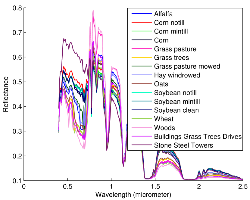
Figure 15: Ground truth endmembers for Indian Pines.

From the regions with visibly different colors in Figure 14 and the noticeably different endmember spectra in Figure 15, we set $M=4$ for all the algorithms. The parameters for SCM were set to $\beta_{2}^{\prime}=0.005$, $\rho_{1}^{\prime}=0.05$. The parameters for PCOMMEND were set to 2 clusters with 2 endmembers in each cluster. The results are shown in Figure 16. The abundance maps show that NCM, PCOMMEND present inconsistent abundances in a ground truth region, e.g. soybean mintill, while SCM presents consistent abundances in the same region.

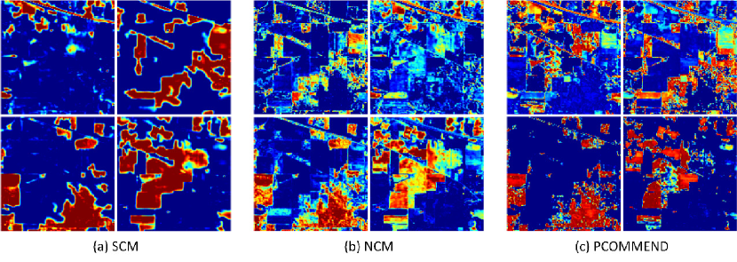
Figure 16: Abundance maps from SCM, NCM and PCOMMEND for Indian Pines.

4 Discussion and Conclusion

In this paper we presented a spatial compositional model (SCM) for linearly unmixing hyperspectral images. The benefits of our model include calculating the full likelihood for uncertainty estimation, a weighted smoothness term on neighboring abundances, and a simple and efficient algorithm that also estimates the endmember uncertainty. The algorithm usually converges within 100 iterations and takes about 2 minutes to process the Pavia University dataset on a laptop with an i7 CPU. The results on synthetic and real datasets show that the estimated endmembers are more accurate than NCM and PCOMMEND. Moreover, the uncertainty encoded by the covariance matrix shows that its range can predict error when the estimated endmembers are inside the pixels. Future work will focus on physically realistic models for hyperspectral unmixing.

Appendix

We show that the objective function (18) can be approximated by (20) for minimization with respect to $\mathbf{A},\,\mathbf{R}$ in this Appendix, i.e.

$$0<\gamma\mathbf{z}^{T}\mathbf{Q}^{-1}\mathbf{z}\ll\gamma\|\mathbf{Y}-\mathbf{A}\mathbf{R}\|_{F}^{2},$$

$$0<\text{log}\left|\mathbf{Q}\right|-\sum_{j=1}^{M}\text{log}\left|\mathbf{S}_{j}\right|\ll\gamma\|\mathbf{Y}-\mathbf{A}\mathbf{R}\|_{F}^{2},$$

given $\gamma,\,\left\{\mathbf{S}_{j}\right\}$ fixed at some optimal values. To be specific, both $\gamma\mathbf{z}^{T}\mathbf{Q}^{-1}\mathbf{z}$ and $\text{log}\left|\mathbf{Q}\right|-\sum_{j=1}^{M}\text{log}\left|\mathbf{S}_{j}\right|$ are in $O\left(MB\right)$ while $\gamma\|\mathbf{Y}-\mathbf{A}\mathbf{R}\|_{F}^{2}$ is in $O\left(NB\right)$. In the applications—Pavia University ($N=207400$, $M=7$) and Indian Pines ($N=21025$, $M=4$)—$\gamma\mathbf{z}^{T}\mathbf{Q}^{-1}\mathbf{z}$ is about 9% and 2% of the least squares term respectively while $\text{log}\left|\mathbf{Q}\right|-\sum_{j=1}^{M}\text{log}\left|\mathbf{S}_{j}\right|$ is about 0.02% and 0.001% respectively.

We first show that $\mathbf{z}^{T}\mathbf{Q}^{-1}\mathbf{z}$ (positive because $\mathbf{Q}\in\text{SPD}\left(MB\right)$) is negligible compared to $\|\mathbf{Y}-\mathbf{A}\mathbf{R}\|_{F}^{2}$. Assume $\mathbf{A}^{T}\mathbf{A}$ is nonsingular (hence $\mathbf{A}^{T}\mathbf{A}\otimes\mathbf{I}_{B}\in\text{SPD}\left(MB\right)$), from the inequality in Lemma 1 (given at the end of this Appendix), we have

$$\mathbf{z}^{T}\mathbf{Q}^{-1}\mathbf{z} = \mathbf{z}^{T}\left(\left[\delta_{ij}\mathbf{S}_{j}\right]+\mathbf{A}^{T}\mathbf{A}\otimes\mathbf{I}_{B}\right)^{-1}\mathbf{z}$$

$$< \mathbf{z}^{T}\left(\mathbf{A}^{T}\mathbf{A}\otimes\mathbf{I}_{B}\right)^{-1}\mathbf{z}$$

$$= \mathbf{z}^{T}\left(\left(\mathbf{V}\boldsymbol{\Lambda}\right)^{-T}\otimes\mathbf{I}_{B}\right)\left(\left(\mathbf{V}\boldsymbol{\Lambda}\right)^{-1}\otimes\mathbf{I}_{B}\right)\mathbf{z}$$

$$= \|\text{vec}\left(\left(\mathbf{Y}-\mathbf{A}\mathbf{R}\right)^{T}\mathbf{A}\left(\mathbf{V}\boldsymbol{\Lambda}\right)^{-T}\right)\|^{2}$$

$$= \|\text{vec}\left(\left(\mathbf{Y}-\mathbf{A}\mathbf{R}\right)^{T}\mathbf{U}\right)\|^{2}$$

$$= \|\mathbf{U}^{T}\left(\mathbf{Y}-\mathbf{A}\mathbf{R}\right)\|_{F}^{2}$$

where $\mathbf{A}=\mathbf{U}\boldsymbol{\Lambda}\mathbf{V}^{T}$, $\mathbf{U}\in\mathbb{R}^{N\times M}$, $\boldsymbol{\Lambda}\in\mathbb{R}^{M\times M}$, $\mathbf{V}\in\mathbb{R}^{M\times M}$ is the compact singular value decomposition (SVD) of $\mathbf{A}$. Since $\mathbf{U}^{T}$ is part of an orthogonal matrix, $\mathbf{U}^{T}\left(\mathbf{Y}-\mathbf{A}\mathbf{R}\right)$ can be seen as rotating the columns of $\mathbf{Y}-\mathbf{A}\mathbf{R}$ and picking only $M$ elements of the rotated vectors, it is trivial compared to $\|\mathbf{Y}-\mathbf{A}\mathbf{R}\|_{F}^{2}$ which has $N$ elements for each column of $\mathbf{Y}-\mathbf{A}\mathbf{R}$.

Second we can show that $\text{log}\left|\mathbf{Q}\right|-\sum_{j=1}^{M}\text{log}\left|\mathbf{S}_{j}\right|>0$ and it is also negligible compared to $\gamma\|\mathbf{Y}-\mathbf{A}\mathbf{R}\|_{F}^{2}$. The positivity arises from Weyl’s inequality (Theorem 4.3.1 in [15]) as the eigenvalues of $\mathbf{Q}$ are greater than those of $\left[\delta_{ij}\mathbf{S}_{j}\right]$. Note that

$$\text{log}\left|\mathbf{Q}\right| = \text{log}\left|\left[\delta_{ij}\mu^{2}\boldsymbol{\Sigma}_{j}^{-1}\right]+\mathbf{A}^{T}\mathbf{A}\otimes\mathbf{I}_{B}\right|$$

$$= \text{log}\mu^{2MB}\left|\left[\delta_{ij}\boldsymbol{\Sigma}_{j}^{-1}\right]+\mu^{-2}\mathbf{A}^{T}\mathbf{A}\otimes\mathbf{I}_{B}\right|$$

$$= -MB\text{log}\gamma+\text{log}\left|\left[\delta_{ij}\boldsymbol{\Sigma}_{j}^{-1}\right]+\gamma\mathbf{A}^{T}\mathbf{A}\otimes\mathbf{I}_{B}\right|,$$

and

$$-\sum_{j=1}^{M}\text{log}\left|\mathbf{S}_{j}\right| = -\sum_{j=1}^{M}\text{log}\left|\mu^{2}\boldsymbol{\Sigma}_{j}^{-1}\right|$$

$$= -\sum_{j=1}^{M}\left\{\text{log}\mu^{2B}+\text{log}\left|\boldsymbol{\Sigma}_{j}^{-1}\right|\right\}$$

$$= MB\text{log}\gamma-\sum_{j=1}^{M}\text{log}\left|\boldsymbol{\Sigma}_{j}^{-1}\right|.$$

Let $\sigma_{j1},...,\sigma_{jB}$ be the the eigenvalues of $\boldsymbol{\Sigma}_{j}^{-1}$ in ascending order and $\lambda_{1},...,\lambda_{M}$ be the eigenvalues of $\mathbf{A}^{T}\mathbf{A}$ in ascending order (so the eigenvalues of $\mathbf{A}^{T}\mathbf{A}\otimes\mathbf{I}_{B}$ are $\lambda_{1},...,\lambda_{M}$ duplicated by $B$ times). The sum of the above two expansions leads to

$$\text{log}\left|\mathbf{Q}\right|-\sum_{j=1}^{M}\text{log}\left|\mathbf{S}_{j}\right|$$

$$= \text{log}\left|\left[\delta_{ij}\boldsymbol{\Sigma}_{j}^{-1}\right]+\gamma\mathbf{A}^{T}\mathbf{A}\otimes\mathbf{I}_{B}\right|-\sum_{j=1}^{M}\text{log}\left|\boldsymbol{\Sigma}_{j}^{-1}\right|$$

$$\leq \text{log}\prod_{j=1}^{M}\prod_{k=1}^{B}\left(\sigma_{jk}+\gamma\lambda_{M}\right)-\sum_{j=1}^{M}\text{log}\prod_{k=1}^{B}\sigma_{jk}$$

$$= \sum_{j=1}^{M}\sum_{k=1}^{B}\text{log}\left(1+\gamma\lambda_{M}/\sigma_{jk}\right)$$

where Weyl’s inequality for the eigenvalues is again used. Given that the reflectances of the endmember signatures are in the range $[0,1]$ (a real hyperspectral image is usually normalized during preprocessing), the endmember covariance matrix should have $\sigma_{jk}$ bounded from below. Although the inside of the logarithm is large, the logarithm makes it limited. Compared with $\gamma\|\mathbf{Y}-\mathbf{A}\mathbf{R}\|_{F}^{2}\approx NB$ with $\gamma$ given in (24), $\sum_{j=1}^{M}\sum_{k=1}^{B}\text{log}\left(1+\gamma\lambda_{M}/\sigma_{jk}\right)$ is negligible considering $M\ll N$.

Lemma 1.

Let $\mathbf{A}\in\text{SPD}\left(n\right)$, $\mathbf{B}\in\text{SPD}\left(n\right)$, for any nonzero $\mathbf{x}\in\mathbb{R}^{n}$, then $\mathbf{x}^{T}\left(\mathbf{A}+\mathbf{B}\right)^{-1}\mathbf{x}<\mathbf{x}^{T}\mathbf{A}^{-1}\mathbf{x}$.

Proof.

Let $\mathbf{A}=\mathbf{U}\boldsymbol{\Sigma}\mathbf{U}^{T}$, $\mathbf{B}=\mathbf{V}\boldsymbol{\Lambda}\mathbf{V}^{T}$ be the eigendecomposition of $\mathbf{A}$ and $\mathbf{B}$ respectively. Then

$$\mathbf{x}^{T}\mathbf{A}^{-1}\mathbf{x}=\mathbf{x}^{T}\left(\mathbf{U}\boldsymbol{\Sigma}\mathbf{U}^{T}\right)^{-1}\mathbf{x}=\mathbf{y}^{T}\boldsymbol{\Sigma}^{-1}\mathbf{y}$$

where $\mathbf{y}=\mathbf{U}^{T}\mathbf{x}$, while

$$\mathbf{x}^{T}\left(\mathbf{A}+\mathbf{B}\right)^{-1}\mathbf{x} = \mathbf{x}^{T}\left(\mathbf{U}\left(\boldsymbol{\Sigma}+\mathbf{Q}\boldsymbol{\Lambda}\mathbf{Q}^{T}\right)\mathbf{U}^{T}\right)^{-1}\mathbf{x}$$

$$= \mathbf{y}^{T}\left(\boldsymbol{\Sigma}+\mathbf{Q}\boldsymbol{\Lambda}\mathbf{Q}^{T}\right)^{-1}\mathbf{y}$$

where $\mathbf{Q}=\mathbf{U}^{T}\mathbf{V}$. By the Woodbury identity,

$$\left(\boldsymbol{\Sigma}+\mathbf{Q}\boldsymbol{\Lambda}\mathbf{Q}^{T}\right)^{-1}=\boldsymbol{\Sigma}^{-1}-\boldsymbol{\Sigma}^{-1}\mathbf{Q}\mathbf{C}\mathbf{Q}^{T}\boldsymbol{\Sigma}^{-1}$$

where

$$\mathbf{C}=\left(\boldsymbol{\Lambda}^{-1}+\mathbf{Q}^{T}\boldsymbol{\Sigma}^{-1}\mathbf{Q}\right)^{-1},$$

we have

$$\mathbf{y}^{T}\left(\boldsymbol{\Sigma}+\mathbf{Q}\boldsymbol{\Lambda}\mathbf{Q}^{T}\right)^{-1}\mathbf{y}=\mathbf{y}^{T}\boldsymbol{\Sigma}^{-1}\mathbf{y}-\mathbf{z}^{T}\mathbf{C}\mathbf{z}$$

where $\mathbf{z}=\mathbf{Q}^{T}\boldsymbol{\Sigma}^{-1}\mathbf{y}$. Because $\mathbf{C}\in\text{SPD}\left(n\right)$ (since $\boldsymbol{\Lambda}^{-1}\in\text{SPD}\left(n\right)$ and $\mathbf{Q}^{T}\boldsymbol{\Sigma}^{-1}\mathbf{Q}\in\text{SPD}\left(n\right)$) and $\mathbf{z}$ is nonzero, $\mathbf{z}^{T}\mathbf{C}\mathbf{z}>0$. Then we have $\mathbf{x}^{T}\left(\mathbf{A}+\mathbf{B}\right)^{-1}\mathbf{x}<\mathbf{x}^{T}\mathbf{A}^{-1}\mathbf{x}$. ∎

References

- [1] P.-A. Absil and J. Malick. Projection-like retractions on matrix manifolds. SIAM Journal on Optimization, 22(1):135–158, 2012.
- [2] A. Baldridge, S. Hook, C. Grove, and G. Rivera. The ASTER spectral library version 2.0. Remote Sensing of Environment, 113(4):711–715, 2009.
- [3] R. H. Bartels and G. Stewart. Solution of the matrix equation . Communications of the ACM, 15(9):820–826, 1972.
- [4] M. Berman, H. Kiiveri, R. Lagerstrom, A. Ernst, R. Dunne, and J. F. Huntington. ICE: A statistical approach to identifying endmembers in hyperspectral images. IEEE Trans. on Geoscience and Remote Sensing, 42(10):2085–2095, 2004.
- [5] D. P. Bertsekas. Nonlinear programming. Athena Scientific, 1999.
- [6] J. M. Bioucas-Dias, A. Plaza, N. Dobigeon, M. Parente, Q. Du, P. D. Gader, and J. Chanussot. Hyperspectral unmixing overview: Geometrical, statistical, and sparse regression-based approaches. IEEE Journal of Selected Topics in Applied Earth Observations and Remote Sensing, 5(2):354–379, 2012.
- [7] D. Cai, X. He, J. Han, and T. S. Huang. Graph regularized nonnegative matrix factorization for data representation. Pattern Analysis and Machine Intelligence, IEEE Transactions on, 33(8):1548–1560, 2011.
- [8] J. Duchi, S. Shalev-Shwartz, Y. Singer, and T. Chandra. Efficient projections onto the -ball for learning in high dimensions. In Proceedings of the 25th international conference on Machine learning, pages 272–279. ACM, 2008.
- [9] O. Eches, N. Dobigeon, C. Mailhes, and J.-Y. Tourneret. Bayesian estimation of linear mixtures using the normal compositional model: Application to hyperspectral imagery. IEEE Trans. Image Processing, 19(6):1403–1413, 2010.
- [10] O. Eches, N. Dobigeon, and J.-Y. Tourneret. Estimating the number of endmembers in hyperspectral images using the normal compositional model and a hierarchical Bayesian algorithm. Selected Topics in Signal Processing, IEEE Journal of, 4(3):582–591, 2010.
- [11] O. Eches, N. Dobigeon, and J.-Y. Tourneret. Enhancing hyperspectral image unmixing with spatial correlations. IEEE Trans. on Geoscience and Remote Sensing, 49(11):4239–4247, 2011.
- [12] A. El Guennouni, K. Jbilou, and A. Riquet. Block Krylov subspace methods for solving large Sylvester equations. Numerical Algorithms, 29(1-3):75–96, 2002.
- [13] N. Guan, D. Tao, Z. Luo, and B. Yuan. Manifold regularized discriminative nonnegative matrix factorization with fast gradient descent. Image Processing, IEEE Transactions on, 20(7):2030–2048, 2011.
- [14] W. W. Hager and S. Park. The gradient projection method with exact line search. Journal of Global Optimization, 30(1):103–118, 2004.
- [15] R. A. Horn and C. R. Johnson. Matrix analysis. Cambridge university press, 1985.
- [16] M.-D. Iordache, J. M. Bioucas-Dias, and A. Plaza. Total variation spatial regularization for sparse hyperspectral unmixing. IEEE Trans. on Geoscience and Remote Sensing, 50(11):4484–4502, 2012.
- [17] S. Jia and Y. Qian. Constrained nonnegative matrix factorization for hyperspectral unmixing. Geoscience and Remote Sensing, IEEE Transactions on, 47(1):161–173, 2009.
- [18] N. Keshava and J. F. Mustard. Spectral unmixing. IEEE Signal Processing Magazine, 19(1):44–57, 2002.
- [19] C.-J. Lin. Projected gradient methods for nonnegative matrix factorization. Neural computation, 19(10):2756–2779, 2007.
- [20] X. Lu, H. Wu, Y. Yuan, P.-g. Yan, and X. Li. Manifold regularized sparse NMF for hyperspectral unmixing. Geoscience and Remote Sensing, IEEE Transactions on, 51(5):2815–2826, 2013.
- [21] L. Miao and H. Qi. Endmember extraction from highly mixed data using minimum volume constrained nonnegative matrix factorization. Geoscience and Remote Sensing, IEEE Transactions on, 45(3):765–777, 2007.
- [22] J. M. Nascimento and J. M. Bioucas Dias. Vertex component analysis: A fast algorithm to unmix hyperspectral data. Geoscience and Remote Sensing, IEEE Transactions on, 43(4):898–910, 2005.
- [23] Y. Qian, S. Jia, J. Zhou, and A. Robles-Kelly. Hyperspectral unmixing via sparsity-constrained nonnegative matrix factorization. Geoscience and Remote Sensing, IEEE Transactions on, 49(11):4282–4297, 2011.
- [24] D. Stein. Application of the normal compositional model to the analysis of hyperspectral imagery. In Advances in Techniques for Analysis of Remotely Sensed Data, 2003 IEEE Workshop on, pages 44–51. IEEE, 2003.
- [25] U. von Luxburg. A tutorial on spectral clustering. Statistics and Computing, 17(4):395–416, 2007.
- [26] A. Zare and P. D. Gader. PCE: Piecewise convex endmember detection. IEEE Trans. on Geoscience and Remote Sensing, 48(6):2620–2632, 2010.
- [27] A. Zare, P. D. Gader, O. Bchir, and H. Frigui. Piecewise convex multiple-model endmember detection and spectral unmixing. IEEE Trans. on Geoscience and Remote Sensing, 51(5):2853–2862, 2013.
- [28] A. Zare and K. Ho. Endmember variability in hyperspectral analysis: Addressing spectral variability during spectral unmixing. IEEE Signal Processing Magazine, 31(1):95–104, 2014.
- [29] B. Zhang, L. Zhuang, L. Gao, W. Luo, Q. Ran, and Q. Du. PSO-EM: A hyperspectral unmixing algorithm based on normal compositional model. IEEE Trans. on Geoscience and Remote Sensing, 52(12):7782–7792, 2014.