Supplementary Information for
“Enhanced nonlinear interactions in quantum optomechanics
via mechanical amplification”

I Derivation of the optomechanical Hamiltonian

We start by describing in more details the rotating wave approximation performed on the system Hamiltonian leading to Eq. (1) of the main text. The starting Hamiltonian that describes the coherent dynamics of the undriven two-cavity optomechanical (OM) setup of interest has the following form,

$$\hat{H}=\Delta\hat{b}^{\dagger}\hat{b}-\frac{1}{2}(\lambda\hat{b}^{2}+\lambda^{*}\hat{b}^{{\dagger}2})+g(\hat{a}_{2}^{\dagger}\hat{a}_{1}e^{i(\omega_{2}-\omega_{1})t}+\hat{a}_{1}^{\dagger}\hat{a}_{2}e^{-i(\omega_{2}-\omega_{1})t})(\hat{b}e^{-i\omega_{p}t}+\hat{b}^{\dagger}e^{i\omega_{p}t}).$$ (S1)

$\hat{H}$ is expressed in an interaction picture with respect to the free cavity Hamiltonians ($\omega_{1},\omega_{2}$) and, for the mechanics, with respect to the pump frequency $\omega_{p}$. The best way to show the validity of the rotating wave approximation performed in our work is to first express $\hat{H}$ in terms of the eigenmode of the quadratic part, i.e. the Bogoliubov mode $\hat{\beta}=\hat{b}\cosh r-\hat{b}^{\dagger}\sinh r$. In the interaction picture with respect to the free $\beta$ mode, it reads

$$\hat{H}=g \left[\hat{a}_{2}^{\dagger}\hat{a}_{1}\left(\hat{\beta}\cosh re^{-iE_{\beta}t}+\hat{\beta}^{\dagger}\sinh re^{iE_{\beta}t}\right)e^{-i\delta t}+\textrm{H.c.}\right]$$ (S2a)

$$+g \left[\hat{a}_{2}^{\dagger}\hat{a}_{1}\left(\hat{\beta}^{\dagger}\cosh re^{iE_{\beta}t}+\hat{\beta}\sinh re^{-iE_{\beta}t}\right)e^{i(\omega_{p}+\omega_{21})t}+\textrm{H.c.}\right],$$ (S2b)

with $\omega_{21}=\omega_{2}-\omega_{1}$, $\delta=\omega_{p}-\omega_{21}$ and $E_{\beta}=\Delta/\cosh 2r$. As a consequence, for $\omega_{p}+\omega_{21}\gg E_{\beta},\tilde{g},\delta,\kappa,\gamma$, where $\gamma$ and $\kappa$ are the mechanical resonator (MR) and the cavities damping rates respectively and $\tilde{g}=ge^{r}/2$, the terms oscillating at $\omega_{21}+\omega_{p}\pm E_{\beta}$ [Eq. (S2b)] can be safely neglected compared to the terms oscillating at $\delta\pm E_{\beta}$. In that case, the resulting Hamiltonian,

$$\hat{H}\approx g\hat{a}_{2}^{\dagger}\hat{a}_{1}(\hat{\beta}\cosh re^{-iE_{\beta}t}+\hat{\beta}^{\dagger}\sinh re^{iE_{\beta}t})e^{-i\delta t}+\textrm{H.c.},$$ (S3)

is exactly the Hamiltonian of Eq. (1) of the main text, expressed in the interaction picture with respect to the free $\beta$ mode.

In our scheme, we are particularly interested in large amplifications $r$ and for detunings such that $\delta=0$ ($\omega_{21}=\omega_{p}$). The optimal parameters which then lead to the most pronounced quantum signatures imply $\Delta\gg E_{\beta},\tilde{g},\kappa,\gamma$ and $E_{\beta}\sim\kappa,\tilde{g}$. It is thus possible to choose $\omega_{p}+\omega_{21}=2\omega_{p}$ big enough so that the rotating wave approximation is always valid. For a positive detuning $\Delta>0$, as we have considered all along this work, it constrains $\omega_{M}-\Delta\gg\kappa,\tilde{g},\gamma$. Choosing negative detunings $\Delta<0$ relaxes this constraint but might cause other issues, like the possibility to excite additional mechanical mode with the parametric drive.

In the situation where the parametric drive is turned off ($r=0$), for instance to freeze the dynamics once a negative Wigner function function is obtained (see main text or Sec. IV for details), $E_{\beta}\rightarrow\Delta\gg\kappa,g,\gamma$. In this case, both interaction terms of Eqs. (S2) become off resonant: The term Eq. (S2a) oscillates at frequency $\Delta$ and the one of Eq. (S2b) at the larger frequency $\Delta+2\omega_{p}$. The contribution from Eq. (S2b) can thus be safely neglected for any parametric drive strength.

II Quantum dynamics of the parametrically driven mechanics

II.1 Langevin equation

We now derive and solve the Heisenberg-Langevin equations of motion for the MR parametrically driven at frequency $2\omega_{p}$. At this point, we do not include the optomechanical interaction, i.e. $g=0$ in Eq. (1) of the main text. Using standard input-output formalism Clerk et al. (2010) to include dissipation to a Markovian bath of thermal occupancy $\bar{n}^{\mathrm{th}}_{M}$ and damping rate $\gamma$, we get, in a frame rotating at $\omega_{p}$,

$$\begin{pmatrix}\hat{b}[\omega]\\ \hat{b}^{\dagger}[\omega]\end{pmatrix}=\begin{pmatrix}i(\Delta-\omega)+\frac{\gamma}{2}&-i\lambda\\ i\lambda&-i(\Delta+\omega)+\frac{\gamma}{2}\end{pmatrix}^{-1}\begin{pmatrix}\sqrt{\gamma}\hat{\eta}[\omega]\\ \sqrt{\gamma}\hat{\eta}^{\dagger}[\omega]\end{pmatrix}\equiv\chi[\omega]\begin{pmatrix}\sqrt{\gamma}\hat{\eta}[\omega]\\ \sqrt{\gamma}\hat{\eta}^{\dagger}[\omega]\end{pmatrix}.$$ (S4)

Here, $\hat{\eta}$ corresponds to the annihilation operator of the noise coming from the MR dissipative bath. As is standard, we consider white Gaussian noise with zero mean ($\langle\hat{\eta}\rangle=0$), so that the non-zero correlators are

$$\langle\hat{\eta}^{\dagger}[\omega]\hat{\eta}[\omega^{\prime}]\rangle=2\pi\bar{n}^{\mathrm{th}}_{M}\delta(\omega+\omega^{\prime}),\qquad\langle\hat{\eta}[\omega]\hat{\eta}^{\dagger}[\omega^{\prime}]\rangle=2\pi(\bar{n}^{\mathrm{th}}_{M}+1)\delta(\omega+\omega^{\prime}).$$ (S5)

We now briefly present how the equations of motion (S4) translate in terms of the Bogoliubov mode $\hat{\beta}$ and discuss the consequences on the dissipation of the $\beta$ mode. The Bogoliubov mode is expressed in terms of the noise operator $\hat{\eta}_{\beta}[\omega]=\eta[\omega]\cosh r-\eta^{\dagger}[\omega]\sinh r$ as follows:

$$\begin{pmatrix}\hat{\beta}[\omega]\\ \hat{\beta}^{\dagger}[\omega]\end{pmatrix}=\textbf{M}\begin{pmatrix}\hat{b}[\omega]\\ \hat{b}^{\dagger}[\omega]\end{pmatrix}=\chi_{\beta}[\omega]\begin{pmatrix}\sqrt{\gamma}\hat{\eta}_{\beta}[\omega]\\ \sqrt{\gamma}\hat{\eta}_{\beta}^{\dagger}[\omega]\end{pmatrix},$$ (S6)

with

M $$=\begin{pmatrix}\cosh r&-\sinh r\\ -\sinh r&\cosh r\end{pmatrix}, \chi_{\beta}[\omega] =\textbf{M}\chi[\omega]\textbf{M}^{-1}=\begin{pmatrix}i(E_{\beta}-\omega)+\frac{\gamma}{2}&0\\ 0&-i(E_{\beta}+\omega)+\frac{\gamma}{2}\end{pmatrix}^{-1}.$$ (S7)

The equation of motion Eq. (S6) shows that when the MR ($\hat{b}$) is coupled to a Markovian bath of thermal occupancy $\bar{n}^{\mathrm{th}}_{M}$, the $\beta$ mode is driven by a squeezed reservoir of thermal population $\bar{n}^{\mathrm{th}}_{M}$. However, as this squeezing is far from the $\beta$-mode resonance $E_{\beta}$ (it is at zero frequency in the current rotating frame), it effectively looks like thermal noise with thermal occupation $\bar{n}^{\mathrm{th}}_{\beta}=\bar{n}^{\mathrm{th}}_{M}\cosh 2r+\sinh^{2}r$. This is precisely revealed in the instantaneous covariance matrix of the $\beta$ mode,

$$\langle\hat{\beta}^{\dagger}\hat{\beta}\rangle(t) =\gamma\iint\frac{d\omega}{2\pi}\frac{d\omega^{\prime}}{2\pi}\frac{\langle\hat{\eta}_{\beta}^{\dagger}[\omega^{\prime}]\hat{\eta}_{\beta}[\omega]\rangle e^{-i(\omega+\omega^{\prime})t}}{(i\omega^{\prime}+iE_{\beta}-\gamma/2)(i\omega-iE_{\beta}-\gamma/2)}=\bar{n}^{\mathrm{th}}_{M}\cosh 2r+\sinh^{2}r,$$ (S8a)

$$\langle\hat{\beta}\hat{\beta}\rangle(t) =\gamma\iint\frac{d\omega}{2\pi}\frac{d\omega^{\prime}}{2\pi}\frac{\langle\hat{\eta}_{\beta}[\omega^{\prime}]\hat{\eta}_{\beta}[\omega]\rangle e^{-i(\omega+\omega^{\prime})t}}{(i\omega^{\prime}-iE_{\beta}-\gamma/2)(i\omega-iE_{\beta}-\gamma/2)}=\frac{-i\gamma(\bar{n}^{\mathrm{th}}_{M}+\frac{1}{2})\sinh 2r}{2E_{\beta}-i\gamma}$$ (S8b)

Here, we have used the correlation functions of the MR bath given in Eqs. (S5). The fact that the squeezing of the reservoir is off-resonant with the $\beta$ mode explicitly appears in the pre-factor $\gamma/E_{\beta}$ in Eq. (S8b). In the limit of weak dissipation, i.e. $\gamma/E_{\beta}\ll 1/\sinh 2r$, the $\beta$ mode can thus be considered as being coupled with a damping rate $\gamma$ to a Markovian thermal bath of effective temperature $\bar{n}^{\mathrm{th}}_{\beta}$.

II.2 Estimation of the cavity heating rate

By adding the coupling to the cavities, one can estimate the rate at which the cavities are heated by the amplified mechanical noise $\hat{\eta}_{\hat{\beta}}(t)$. For simplicity, we consider the particular case where the dynamics is well described by $\hat{H}_{\mathrm{SRP}}$ [Eq. (2) of the main text] with $\hat{H}^{\prime}_{\mathrm{SRP}}=0$, i.e. for $\delta=0$, $e^{2r}\gg 1$ and for a $\beta$ mode initially close to its ground state. In this case, the equations of motion are given by:

$$\dot{\hat{\beta}}=-(iE_{\beta}+\tfrac{1}{2}\gamma)\hat{\beta}-i\tilde{g}(\hat{a}_{2}^{\dagger}\hat{a}_{1}+\hat{a}_{1}^{\dagger}\hat{a}_{2})-\sqrt{\gamma}\hat{\eta}_{\hat{\beta}},$$ (S9a)

$$\dot{\hat{a}}_{1,2}=-\tfrac{1}{2}\kappa\hat{a}_{1,2}-i\tilde{g}\hat{a}_{2,1}(\hat{\beta}+\hat{\beta}^{\dagger})-\sqrt{\kappa}\hat{\xi}_{1,2}.$$ (S9b)

Here, $\hat{\xi}_{1,2}$ represents standard Gaussian noise entering cavity $1,2$. In this rotating frame, the dominant contributions of the mechanics on the cavity dynamics come from the low frequencies. Given the fast dynamics of the MR ($E_{\beta}\gg\kappa,\tilde{g}$), one can solve the equation of motion of the MR adiabatically, i.e. for $\dot{\hat{\beta}}=0$. If we then substitute this solution into Eq. (S9b) to eliminate $\hat{\beta}$ from the cavity equation of motion, one obtains an equation for the cavities that explicitly shows how the mechanical bath couples to the cavities. For $\gamma\ll E_{\beta}$, the mechanical noise generates a contribution for $\dot{\hat{a}}_{1,2}$ of the form $\frac{\tilde{g}}{E_{\beta}}\sqrt{\gamma}\hat{a}_{2,1}(\hat{\eta}_{\hat{\beta}}-\hat{\eta}_{\hat{\beta}}^{\dagger})$. In a mean field approximation, one can then roughly approximate the rate $\Gamma_{i}$ at which the mechanics heats the cavity $i$, which reads:

$$\Gamma_{i}\sim\gamma\frac{\tilde{g}^{2}}{E_{\beta}^{2}}\bar{n}_{j}(2\bar{n}^{\mathrm{th}}_{\beta}+1)\approx\gamma\frac{g^{2}}{E_{\beta}^{2}}\bar{n}_{j}(2\bar{n}^{\mathrm{th}}_{M}+1)e^{4r}.$$ (S10)

Here $\bar{n}_{j}$ represents the mean number of photons in cavity $j=2,1$ for $i=1,2$. For a MR coupled to a thermal bath of temperature $\bar{n}^{\mathrm{th}}_{M}$ and parametrically driven such that $e^{2r}\gg 1$, $\Gamma_{i}$ gives an estimate of the rate at which the cavity $i$, coupled to the MR via the single-photon coupling constant $g$, is heated.

II.3 Non-interacting mechanical Green’s functions

We calculate the non-interacting mechanical Green’s function from the equations of motion (S4). In terms of the $\chi[\omega]$ matrix, the retarded Green’s functions are,

$$G^{R}_{b}[\omega]=\int_{-\infty}^{\infty}\mathrm{d}tG^{R}_{b}(t)e^{i\omega t}=-i\chi_{1,1}[\omega]=\frac{\cosh^{2}r}{\omega-E_{\beta}+i\gamma/2}-\frac{\sinh^{2}r}{\omega+E_{\beta}+i\gamma/2},$$ (S11a)

$$\tilde{G}^{R}_{b}[\omega]=\int_{-\infty}^{\infty}\mathrm{d}t\tilde{G}^{R}_{b}(t)e^{i\omega t}=i\chi_{1,2}[\omega]=\frac{\sinh 2r}{2}\left(\frac{1}{\omega-E_{\beta}+i\gamma/2}-\frac{1}{\omega+E_{\beta}+i\gamma/2}\right).$$ (S11b)

Without the parametric drive, the off-diagonal Green’s function $\tilde{G}^{R}_{b}[\omega]$ vanishes. In the large $r$ limit ($e^{2r}\gg 1$) and for weak dissipation ($\gamma\ll E_{\beta}$), $G^{R}_{b}[\omega]=\tilde{G}^{R}_{b}[\omega]$.

As we work in the interaction picture for the cavities, the shortest time scales relevant to the photons are $1/\kappa,1/\tilde{g}$. Hence, the important contributions of the MR Green’s functions to the effective two-photon interaction occur at low frequencies, i.e. $\omega\ll\kappa,\tilde{g}$. Consequently, to amplify the photon-photon interaction, one can decrease the parametric drive detuning $\Delta$ and increase its strength $\lambda$, which lowers the energy $E_{\beta}$ and increases the exponential amplification $r$. However, to ensure that the interaction is sufficiently broadband, in other words local in time, one always needs to have $E_{\beta}>\kappa,\tilde{g}$.

The non-interacting Keldysh Green’s function of the MR are

$$G^{K}_{b}[\omega] =-i\gamma(2\bar{n}^{\mathrm{th}}_{M}+1)(|\chi_{11}[\omega]|^{2}+|\chi_{12}[\omega]|^{2}),$$ (S12a)

$$\tilde{G}^{K}_{b}[\omega] =-i\gamma(2\bar{n}^{\mathrm{th}}_{M}+1)(\chi_{11}[\omega]\chi_{21}^{*}[\omega]+\chi_{12}[\omega]\chi_{22}^{*}[\omega]).$$ (S12b)

Their expressions are awkward, therefore we only focus on the limit $e^{2r}\gg 1$ and $\gamma\ll E_{\beta}$. In these limits, one gets,

$$G^{K}_{b}[\omega]=\tilde{G}^{K}_{b}[\omega]=(1+2\bar{n}^{\mathrm{th}}_{M})\frac{e^{4r}}{8}\left(\frac{1}{\omega-E_{\beta}+i\gamma/2}+\frac{1}{\omega+E_{\beta}+i\gamma/2}-\frac{1}{\omega-E_{\beta}-i\gamma/2}-\frac{1}{\omega+E_{\beta}-i\gamma/2}\right).$$ (S13)

As discussed above, The Keldysh Green functions capture the fact that the MR produces additional noises on the cavities. As in the case of the retarded Green functions, when $G^{K}_{b}[\omega]$ is peaked far from any relevant frequencies for the cavities dynamics, i.e. $E_{\beta}>\kappa,\tilde{g}$, the additional noise is off-resonant and scale as $\frac{\gamma}{E_{\beta}}(1+2\bar{n}^{\mathrm{th}}_{M})e^{4r}$.

III Non-Gaussian cavity states

The non-Gaussian character of the cavity state is addressed in Fig. S1, where the $g_{a_{s}}^{(2)}(0)$ correlation functions plotted in Fig. 3 of the main text are compared to the result that would be obtained if the states were Gaussian. In the case of purely Gaussian states, it is possible to calculate $g_{a_{s}}^{(2)}(0)$ solely in terms of the covariance matrix of the cavity state, i.e. by using Wick’s theorem Lemonde et al. (2014). The results for the Gaussian state presented in Fig. S1 thus consist of calculating the covariance matrix of the optical state and extrapolating the corresponding $g_{a_{s}}^{(2)}(0)$ via a Wick expansion of the term $\langle\hat{a}_{s}^{{\dagger}2}\hat{a}_{s}^{2}\rangle$. For increasing $g$, the result for the Gaussian state deviates from the full solution, thus explicitly demonstrating that the photons are in a non-Gaussian state, and that the $g_{a_{s}}^{(2)}(0)$ suppression is due to true photon blockade. As expected, as the nonlinearity vanishes $g\rightarrow 0$, the optical state becomes purely Gaussian.

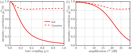
Figure S1: Comparison between the $g_{a_{s}}^{(2)}(0)$ correlation function for Hamiltonian $\hat{H}_{\mathrm{SRP}}$ with the parameters of Fig. 3 of the main text (full lines) and the intensity correlation supposing Gaussian optical states (dashed lines). The Gaussian result only involves the expectation values $\langle\hat{a}_{s}\rangle$, $\langle\hat{a}_{s}^{\dagger}\hat{a}_{s}\rangle$ and $\langle\hat{a}_{s}^{2}\rangle$. The clear different indicates that the enhanced photon-photon interaction induces non-Gaussian photonic states. This is reminiscent of true photon antibunching due to the nonlinear interaction.

IV Emission of cavity states to input/output waveguide

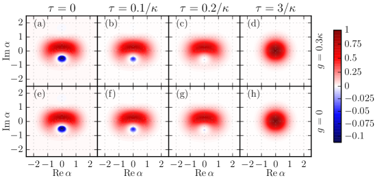
Figure S2: Decay dynamics of a quantum state after the parametric drive is switched off with the TD scheme. The initial state corresponds to the Wigner function plotted in Fig. 4 (c) of the main text [panels (a) and (e) here]. The decay of this initial state in cavity 1 in presence of the residual optomechanical coupling $g=0.3\kappa$ (c-d) is compared to the non-interacting cavity $g=0$ (f-h) at different times. The two dynamics are identical, ensuring that the quantum state is perfectly transferred to propagating photons.

The protocol to prepare negative optical Wigner functions explained in the main text shows the intracavity dynamics. As discussed, by turning off the parametric drive rapidly using a transitionless driving (TD) scheme, the optomechanical interaction is effectively turned off, and the intracavity state is converted into a propagating state. We show here that once the parametric drive is turned off, the remaining weak optomechanical coupling $g$ plays no role in the dynamics (both because it is not enhanced by the coupling, and because it is now non-resonant). The Hamiltonian is then given by Eq. (1) of the main text with $\lambda=0$,

$$\hat{H}=\Delta\hat{b}^{\dagger}\hat{b}+g[\hat{a}_{1}\hat{a}_{2}^{\dagger}\hat{b}+\hat{a}_{1}^{\dagger}\hat{a}_{2}\hat{b}^{\dagger}].$$ (S14)

The nonlinear interaction is weak ($g$ instead of $\tilde{g}$) and strongly off resonant ($\Delta$ instead of $E_{\beta}\ll\Delta$). Moreover, in the absence of excitation for both the MR and cavity 2, the interaction is suppressed, thereby preventing the residual nonlinear interaction from affecting the dynamics of the cavity-1 state. Finally, the non-rotating wave term that is neglected in Eq. (S14) (involving $\hat{a}_{2}^{\dagger}\hat{a}_{1}\hat{b}^{\dagger}$) remains negligible as it is highly non-resonant [see text after Eq. (S3)].

The decay dynamics is shown in Fig. S2 for $g=0.3\kappa$ and compared to the decay of the non-interacting cavity (i.e. for $g=0$). The Wigner functions are identical and the fidelity between the two evolutions stays at 1. This agreement ensures that the initial quantum state is perfectly transferred to the propagating photons of the outgoing field and can be sent to remote quantum systems.

V Parametrically driving the cavity

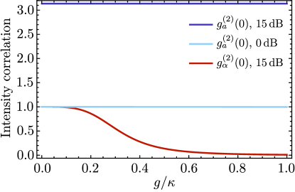
Figure S3: Intensity correlation functions of the parametrically driven cavity mode as a function of the OM coupling $g$. We compare the $g^{(2)}(0)$ function of the $\alpha$ mode (red line) to the real photon $\hat{a}$ (dark blue) for an amplification of $15\,\mathrm{dB}$. We see that while $g^{(2)}(0)$ goes below $1$ for the $\alpha$ mode, there is no suppression for the real photons. More precisely, the parametric drive increases the intensity correlation of the real photons, as can be seen by comparing to $g^{(2)}_{a}(0)$ without parametric drive (light blue line). The parameters used are $\omega_{M}=50\kappa$, $\omega_{d}=-g^{2}\cosh^{2}(2r_{c})/\omega_{M}$, $\epsilon=0.001\kappa$, $\gamma=10^{-4}\kappa$ and zero temperature dissipative baths for the MR and the $\alpha$ mode.

In our work, we consider how parametric mechanical driving enhances the interaction in an OM system. The dual situation was studied recently by Xin-You Lü et al. in Ref. Lü et al., 2015, where the cavity in an OM system is parametrically driven. Because the OM interaction [$\propto\hat{a}^{\dagger}\hat{a}(\hat{b}^{\dagger}+\hat{b})$, see Eq. (S15)] is fundamentally asymmetric between photons and phonons, the photons, unlike the phonons, do not mediate any effective interaction. Parametrically driving the cavity thus gives rise to a different physics and, in particular, does not lead to the enhancement of the nonlinear interaction at the single-photon level. We explain this point in more details here, and show explicitly that the approach of Ref. Lü et al., 2015 does not result in a photonic intensity correlation function satisfying $g^{(2)}(0)<1$.

For simplicity, we consider a single cavity mode coupled to the MR as it is studied in Ref. Lü et al., 2015. The corresponding coherent dynamics is governed by the following Hamiltonian,

$$\hat{H}=\Delta\hat{a}^{\dagger}\hat{a}-\tfrac{1}{2}\lambda(\hat{a}\hat{a}+\hat{a}^{\dagger}\hat{a}^{\dagger})+\omega_{M}\hat{b}^{\dagger}\hat{b}+g\hat{a}^{\dagger}\hat{a}(\hat{b}+\hat{b}^{\dagger}).$$ (S15)

Here $\Delta=\omega_{\mathrm{c}}-\omega_{p}$ with $\omega_{\mathrm{c}}$, $2\omega_{p}$ being respectively the cavity and the parametric drive frequencies and $\lambda$ is the parametric drive strength. We treat the squeezed photons as we treated the parametrically driven phonons in the text. We diagonalize the quadratic part of $\hat{H}$ by applying the Bogoliubov transformation $\hat{a}=\cosh r\hat{\alpha}+\sinh r\hat{\alpha}^{\dagger}$ with $\tanh 2r=\lambda/\Delta$. In this squeezed basis, the energy of the $\alpha$-mode is $E_{\alpha}=\Delta/\cosh(2r_{\mathrm{c}})$ and the Hamiltonian reads,

$$\hat{H}=E_{\alpha}\hat{\alpha}^{\dagger}\hat{\alpha}+\omega_{M}\hat{b}^{\dagger}\hat{b}+g\cosh(2r_{\mathrm{c}})\hat{\alpha}^{\dagger}\hat{\alpha}(\hat{b}^{\dagger}+\hat{b})+\tfrac{1}{2}g\sinh(2r_{\mathrm{c}})(\hat{\alpha}\hat{\alpha}+\hat{\alpha}^{\dagger}\hat{\alpha}^{\dagger})(\hat{b}^{\dagger}+\hat{b}).$$ (S16)

As in Ref. Lü et al., 2015, we focus on the limit $E_{\alpha}\gg\omega_{M},g\sinh(2r_{\mathrm{c}})$ and neglect the off-resonant nonlinear interaction [last term of Eq. (S16)]. After eliminating the mechanical degree of freedom with a polaron transformation $\hat{U}=\exp[g\cosh(2r_{\mathrm{c}})(\hat{b}^{\dagger}-\hat{b})\hat{\alpha}^{\dagger}\hat{\alpha}/\omega_{M}]$, the OM interaction generates a Kerr nonlinearity for the $\alpha$ mode of the form

$$\hat{H}_{\mathrm{pol}}=\hat{U}\hat{H}\hat{U}^{\dagger}=E_{\alpha}\hat{\alpha}^{\dagger}\hat{\alpha}+\omega_{M}\hat{b}^{\dagger}\hat{b}-K_{\mathrm{c}}(\hat{\alpha}^{\dagger}\hat{\alpha})^{2},$$ (S17)

with $K_{\mathrm{c}}=g^{2}\cosh^{2}(2r_{\mathrm{c}})/\omega_{M}$. It thus follows that photonic parametric driving leads to an extremely nonlinear energy spectrum (similar to our approach). However, the eigenstates corresponding to the nonlinearity in Eq. (S17) are not few photon states; they are $\alpha$-mode Fock states, and correspond to squeezed photonic Fock state. They thus necessarily involve extremely large photon numbers when $r_{\mathrm{c}}\gg 1$. Thus, to make use of the nonlinearity in Eq. (S17) one must necessarily work with states with large photon number. This is in stark contrast to our scheme, where the enhanced nonlinear spectrum corresponds to states having only a few photons.

This difference in the eigenstates associated with the enhanced nonlinearity is not just a question of semantics: it leads to crucial observable differences. As an example, we consider again the $g^{(2)}(0)$ intensity correlation function of the cavity photons. As in Ref. Lü et al., 2015, we consider a weak drive of the form $\hat{H}_{\mathrm{drive}}=\epsilon(\hat{a}e^{i\omega_{d}t}+\mathrm{H.c.})$, with frequency $\omega_{d}$ in the frame rotating at $\omega_{p}$, to probe the intensity fluctuations of the cavity. For a very weak drive ($\epsilon\ll g$) that is near resonance with the Bogoliubov mode (small detuning $\delta_{\alpha}=E_{\alpha}-\omega_{d}$), the drive term reduces to $\hat{H}_{\mathrm{drive}}\approx\epsilon\cosh r(\hat{\alpha}e^{i\omega_{d}t}+\mathrm{H.c.})$. In the frame rotating at $\omega_{d}+\omega_{p}$, one gets the following final Hamiltonian,

$$\hat{H}=\delta_{\alpha}\hat{\alpha}^{\dagger}\hat{\alpha}+\omega_{M}\hat{b}^{\dagger}\hat{b}+g\cosh(2r_{\mathrm{c}})\hat{\alpha}^{\dagger}\hat{\alpha}(\hat{b}^{\dagger}+\hat{b})+\epsilon\cosh r_{\mathrm{c}}(\hat{\alpha}+\hat{\alpha}^{\dagger}).$$ (S18)

We use a standard Lindblad master equation to calculate the equal-time intensity correlation function of the cavity under the dynamics of the Hamiltonian Eq. (S18) and we consider that both the mechanical mode and the $\alpha$ mode are coupled to zero temperature baths. Zero temperature dissipation for the $\alpha$ mode is possible if the cavity is also driven by squeezed light with a properly tuned phase Lü et al. (2015).

In Fig. S3, we compare the real photon intensity correlation $g^{(2)}_{a}(0)$ to the $\alpha$ mode intensity correlation $g^{(2)}_{\alpha}(0)$ as a function of $g$ for an amplification of $15\,\mathrm{dB}$ [i.e. $e^{2r}\simeq 32$]. As expected from the Kerr interaction in Eq. (S17), $g^{(2)}_{\alpha}(0)$ drops rapidly below $1$ as $g$ is increased. However, it is not the case for the real photons ($\hat{a}$): even with no additional coherent drive, the large photon population in the cavity induced by the parametric drive would yield $g^{(2)}_{a}(0)\sim 3$. Physically speaking, the effects of the enhanced nonlinear interaction on the cavity are sitting on top of a large photon-number Gaussian state, making them both hard to detect and exploit. This is again in stark contrast to our scheme, where there is no large background number of photons obscuring the interesting physics. Furthermore, the relevant observable directly measured by a photodetector is $g_{a}^{2}(0)$, not the $g_{\alpha}^{2}(0)$ intensity correlation of the $\alpha$ mode.

Finally, it is worth noting that the scheme of Ref. Lü et al., 2015 would apply to any system having a weak Kerr interaction, and does not make use of any special aspect of an optomechanical system; parametrically driven Kerr cavities have been studied far earlier in the literature, see e.g. Ref. Wielinga and Milburn, 1994. On a heuristic level, parametrically driving the cavity puts it in a state with a large number of photons in it; given this large population, it is not surprising that any intrinsic weak nonlinearity will play a larger role.

References

• Clerk et al. (2010) A. A. Clerk, M. H. Devoret, S. M. Girvin, F. Marquardt, and R. J. Schoelkopf, Rev. Mod. Phys. 82, 1155 (2010).
• Lemonde et al. (2014) M.-A. Lemonde, N. Didier, and A. A. Clerk, Phys. Rev. A 90, 063824 (2014).
• Lü et al. (2015) X.-Y. Lü, Y. Wu, J. R. Johansson, H. Jing, J. Zhang, and F. Nori, Phys. Rev. Lett. 114, 093602 (2015).
• Wielinga and Milburn (1994) B. Wielinga and G. J. Milburn, Phys. Rev. A 49, 5042 (1994).