On the quasi-unconditional stability of BDF-ADI solvers for the compressible Navier-Stokes equations

Abstract

The companion paper “Higher-order in time quasi-unconditionally stable ADI solvers for the compressible Navier-Stokes equations in 2D and 3D curvilinear domains”, which is referred to as Part I in what follows, introduces ADI (Alternating Direction Implicit) solvers of higher orders of temporal accuracy (orders $s=2$ to 6) for the compressible Navier-Stokes equations in two- and three-dimensional space. The proposed methodology employs the backward differentiation formulae (BDF) together with a quasilinear-like formulation, high-order extrapolation for nonlinear components, and the Douglas-Gunn splitting. A variety of numerical results presented in Part I demonstrate in practice the theoretical convergence rates enjoyed by these algorithms, as well as their excellent accuracy and stability properties for a wide range of Reynolds numbers. In particular, the proposed schemes enjoy a certain property of “quasi-unconditional stability”: for small enough (problem-dependent) fixed values of the time-step $\Delta t$, these algorithms are stable for arbitrarily fine spatial discretizations. The present contribution presents a mathematical basis for the performance of these algorithms. Short of providing stability theorems for the full BDF-ADI Navier-Stokes solvers, this paper puts forth proofs of unconditional stability and quasi-unconditional stability for BDF-ADI schemes as well as some related un-split BDF schemes, for a variety of related linear model problems in one, two and three spatial dimensions, and for schemes of orders $2\leq s\leq 6$ of temporal accuracy. Additionally, a set of numerical tests presented in this paper for the compressible Navier-Stokes equation indicate that quasi-unconditional stability carries over to the fully non-linear context.

1 Introduction

The companion paper [4], which is referred to as Part I in what follows, introduces ADI (Alternating Direction Implicit) solvers of higher orders of time-accuracy (orders $s=2$ to 6) for the compressible Navier-Stokes equations in two- and three-dimensional curvilinear domains. Implicit solvers, even of ADI type, are generally more expensive per time-step, for a given spatial discretization, than explicit solvers, but use of efficient implicit solvers can be advantageous whenever the time-step restrictions imposed by the mesh spacing $h$ are too severe. The proposed methodology employs the BDF (backward differentiation formulae) multi-step ODE solvers (which are known for their robust stability properties) together with a quasilinear-like formulation and high-order extrapolation for nonlinear components (which gives rise to a linear problem that can be solved efficiently by means of standard linear algebra solvers) and the Douglas-Gunn splitting (an ADI strategy that greatly simplifies the treatment of boundary conditions while retaining the order of time-accuracy of the solver).

As discussed in Part I, the proposed BDF-ADI solvers are the first ADI-based Navier-Stokes solvers for which high-order time-accuracy has been demonstrated. In spite of the nominal second order of time-accuracy inherent in the celebrated Beam and Warming method [1] (cf. also [2, 20]), previous ADI solvers for the Navier-Stokes equations have not demonstrated time-convergence of orders higher than one under general non-periodic physical boundary conditions. Part I demonstrates the properties of the proposed schemes by means of a variety of numerical experiments; the present paper, in turn, provides a theoretical basis for the observed algorithmic stability traits. Restricting attention to linear model problems related to the fully nonlinear Navier-Stokes equations—including the advection-diffusion equation in one, two and three spatial dimensions as well as general parabolic and hyperbolic linear equations in two spatial dimensions—the present contribution provides proofs of unconditional stability for BDF-ADI schemes of second order as well as proofs of quasi-unconditional stability (Definition 1 below) for certain related BDF-based unsplit (non-ADI) schemes of orders $3\leq s\leq 6$. Further, a variety of numerical tests presented in Section 6 indicate that the property of quasi-unconditional stability carries over to the BDF-ADI solvers for the fully non-linear Navier-Stokes equations.

The BDF-ADI methodology mentioned above can be applied in conjunction with a variety of spatial discretizations. For definiteness, in this contribution attention is restricted to Chebyshev, Legendre and Fourier spectral spatial approximations. The resulting one-dimensional boundary value problems arising from these discretizations involve full matrices which generally cannot be inverted efficiently by means of a direct solver. However, by relying on fast transforms these systems can be solved effectively on the basis of the GMRES iterative solver; details in these regards are presented in Part I. Additionally, as detailed in that reference, in order to ensure stability for the fully nonlinear Navier-Stokes equations a mild spectral filter is used.

Perhaps the existence of Dahlquist’s second barrier may explain the widespread use of implicit methods of orders less than or equal to two in the present context (such as backward Euler, the trapezoidal rule and BDF2, all of which are A-stable), and the virtual absence of implicit methods of orders higher than two—despite the widespread use of the fourth order Runge-Kutta and Adams-Bashforth explicit counterparts. Clearly, A-stability is not necessary for all problems—for example, any method whose stability region contains the negative real axis (such as the BDF methods of orders two to six) generally results in an unconditionally stable solver for the heat equation. A number of important questions thus arise: Do the compressible Navier-Stokes equations inherently require A-stability? Are the stability constraints of all higher-order implicit methods too stringent to be useful in the Navier-Stokes context? How close to unconditionally stable can a Navier-Stokes solver be whose temporal order of accuracy is higher than two?

Clear answers to these questions are not available in the extant literature; the present work seeks to provide a theoretical understanding in these regards. To illustrate the present state of the art concerning such matters we mention the 2002 reference [3], which compares various implicit methods for the Navier-Stokes equations, where we read: “Practical experience indicates that large-scale engineering computations are seldom stable if run with BDF4. The BDF3 scheme, with its smaller regions of instability, is often stable but diverges for certain problems and some spatial operators. Thus, a reasonable practitioner might use the BDF2 scheme exclusively for large-scale computations.” It must be noted, however, that neither the article [3] nor the references it cites investigate in detail the stability restrictions associated with the BDF methods order $s\geq 2$, either theoretically or experimentally. But higher-order methods can be useful: as demonstrated in Part I, methods of order higher than two give rise to very significant advantages for certain classes of problems—especially for large-scale computations for which the temporal dispersion inherent in low-order approaches would make it necessary to use inordinately small time-steps.

The recent 2015 article [8], in turn, presents applications of the BDF scheme up to third order of time accuracy in a finite element context for the incompressible Navier-Stokes equations with turbulence modelling. This contribution does not discuss stability restrictions for the third order solver, and, in fact, it only presents numerical examples resulting from use of BDF1 and BDF2. The 2010 contribution [12], which considers a three-dimensional advection-diffusion equation, presents various ADI-type schemes, one of which is based on BDF3. The BDF3 stability analysis in that paper, however, is restricted to the purely diffusive case.

This paper is organized as follows: Section 2 presents a brief derivation of the BDF-ADI method for the two-dimensional pressure-free momentum equation. (A derivation for the full Navier-Stokes equations is given in Part I, but the specialized derivation presented here may prove valuable in view of its relative simplicity.) Section 3 then briefly reviews relevant notions from classical stability theory as well as the concept of quasi-unconditional stability introduced in Part I. Section 4 presents proofs of (classical) unconditional stability for two-dimensional BDF-ADI schemes of order $s=2$ specialized to the linear constant coefficient periodic advection equation as well as the linear constant coefficient periodic and non-periodic parabolic equations. Proofs of quasi-unconditional stability for the (non-ADI) BDF methods of orders $s=2,\dots,6$ applied to the constant coefficient advection-diffusion equation in one, two, and three spatial dimensions are presented in Section 5, along with comparisons of the stability constraints arising from these BDF solvers and the commonly-used explicit Adams-Bashforth solvers of orders three and four. Section 6 provides numerical tests that indicate that the BDF-ADI methods of orders $s=2$ to $6$ for the the full three-dimensional Navier-Stokes equations enjoy the property of quasi-unconditional stability; a wide variety of additional numerical experiments are presented in Part I. Section 7, finally, presents a few concluding remarks.

2 The BDF-ADI scheme

In this section we present a derivation of the BDF-ADI scheme in a somewhat simplified context, restricting attention to the two-dimensional pressure-free momentum equation

$$\mathbf{u}_{t}+\mathbf{u}\cdot\nabla\mathbf{u}=\mu(\,\Delta\mathbf{u}+\frac{1}{3}\nabla(\nabla\cdot\mathbf{u})\,)$$ (1)

in Cartesian coordinates for the velocity vector $\mathbf{u}=(u,v)^{\mathrm{T}}$. The present derivation may thus be more readily accessible than the one presented in Part I for the full Navier-Stokes equations under curvilinear coordinates. Like the BDF-ADI Navier-Stokes algorithms presented in Part I, the schemes discussed in this section incorporate three main elements, namely, 1) A BDF-based time discretization; 2) High-order extrapolation of relevant factors in quasilinear terms (the full compressible Navier-Stokes solver presented in Part I utilizes a similar procedure for non-quasilinear terms); and 3) The Douglas-Gunn ADI splitting.

The semi-discrete BDF scheme of order $s$ for equation (1) is given by

$$\mathbf{u}^{n+1}=\sum_{j=0}^{s-1}a_{j}\mathbf{u}^{n-j}+b\Delta t\left(-\mathbf{u}^{n+1}\cdot\nabla\mathbf{u}^{n+1}+\mu(\,\Delta\mathbf{u}^{n+1}+\frac{1}{3}\nabla(\nabla\cdot\mathbf{u}^{n+1})\,)\right)$$ (2)

where $a_{j}$ and $b$ are the order-$s$ BDF coefficients (see e.g. [14, Ch. 3.12] or Part I); the truncation error associated with this scheme is a quantity of order $\mathcal{O}((\Delta t)^{s+1})$. This equation is quasi-linear: the derivatives of the solution appear linearly in the equation. Of course, the full compressible Navier-Stokes equations contain several non-quasilinear nonlinear terms. As detailed in Part I, by introducing a certain “quasilinear-like” form of the equations, all such nonlinear terms can be treated by an approach similar to the one described in this section. In preparation for a forthcoming ADI splitting we consider the somewhat more detailed form

$$\begin{split}\mathbf{u}^{n+1}=\sum_{j=0}^{s-1}a_{j}\mathbf{u}^{n-j}+b\Delta t\bigg{(}-u^{n+1}\partial_{x}-v^{n+1}&\partial_{y}+\mu\left(\begin{smallmatrix}4/3&0\\ 0&1\end{smallmatrix}\right)\partial_{x}^{2}\\ &+\mu\left(\begin{smallmatrix}1&0\\ 0&4/3\end{smallmatrix}\right)\partial_{y}^{2}+\mu\left(\begin{smallmatrix}0&1/3\\ 1/3&0\end{smallmatrix}\right)\partial_{x}\partial_{y}\bigg{)}\mathbf{u}^{n+1}\end{split}$$ (3)

of equation (2), which we then rewrite as

$$\begin{split}\Bigg{(}I+b\Delta t\bigg{(}u^{n+1}\partial_{x}+v^{n+1}\partial_{y}+\mu\left(\begin{smallmatrix}4/3&0\\ 0&1\end{smallmatrix}\right)&\partial_{x}^{2}+\mu\left(\begin{smallmatrix}1&0\\ 0&4/3\end{smallmatrix}\right)\partial_{y}^{2}\bigg{)}\Bigg{)}\mathbf{u}^{n+1}\\ &=\sum_{j=0}^{s-1}a_{j}\mathbf{u}^{n-j}+b\Delta t\mu\left(\begin{smallmatrix}0&1/3\\ 1/3&0\end{smallmatrix}\right)\partial_{x}\partial_{y}\mathbf{u}^{n+1}.\end{split}$$ (4)

Upon spatial discretization, the solution of equation (4) for the unknown velocity field $\mathbf{u}^{n+1}$ amounts to inversion of a (generally large) non-linear system of equations. In order to avoid inversion of such nonlinear systems we rely on high-order extrapolation of certain non-differentiated terms. This procedure eliminates the nonlinearities present in the equation while preserving the order of temporal accuracy of the algorithm. In detail, let $P_{u}$ (resp. $P_{v}$) denote the polynomial of degree $s-1$ that passes through $(t^{n-j+1},u^{n-j+1})$ (resp. through $(t^{n-j+1},v^{n-j+1})$) for $1\leq j\leq s$, and define $\widetilde{u}_{s}^{n+1}=P_{u}(t^{n+1})$ (resp. $\widetilde{v}_{s}^{n+1}=P_{v}(t^{n+1}$)) and $\mathbf{\widetilde{u}}_{s}^{n+1}=(\widetilde{u}_{s}^{n+1},\widetilde{v}_{s}^{n+1})$. Then, substituting $\widetilde{u}_{s}^{n+1}$ and $\widetilde{v}_{s}^{n+1}$ (resp. $\mathbf{\widetilde{u}}_{s}^{n+1}$) for the un-differentiated terms $u^{n+1}$ and $v^{n+1}$ (resp. for the mixed derivative term) in equation (4), the alternative variable-coefficient linear semi-discrete scheme

$$\bigg{[}I+b\Delta t\bigg{(}\widetilde{u}_{s}^{n+1}\partial_{x}+\widetilde{v}_{s}^{n+1}\partial_{y}+\mu\left(\begin{smallmatrix}4/3&0\\ 0&1\end{smallmatrix}\right)\partial_{x}^{2}+\mu\left(\begin{smallmatrix}1&0\\ 0&4/3\end{smallmatrix}\right)\partial_{y}^{2}\bigg{)}\bigg{]}\mathbf{u}^{n+1}$$

$$=\sum_{j=0}^{s-1}a_{j}\mathbf{u}^{n-j}+b\Delta t\mu\left(\begin{smallmatrix}0&1/3\\ 1/3&0\end{smallmatrix}\right)\partial_{x}\partial_{y}\mathbf{\widetilde{u}}_{s}^{n+1}$$ (5)

results. Clearly the truncation errors inherent in the linear scheme (2) are of the same order as those associated with the original nonlinear scheme (4).

Even though equation (2) is linear, solution of (a spatially discretized version of) this equation requires inversion of a generally exceedingly large linear system at each time step. To avoid this difficulty we resort to a strategy of ADI type [16] and, more explicitly, to the Douglas-Gunn splitting [7]. To derive the Douglas-Gunn splitting we re-express equation (2) in the factored form

$$\bigg{[}I+b\Delta t\bigg{(}\widetilde{u}_{s}^{n+1}\partial_{x}+\mu\left(\begin{smallmatrix}4/3&0\\ 0&1\end{smallmatrix}\right)\partial_{x}^{2}\bigg{)}\bigg{]}\bigg{[}I+b\Delta t\bigg{(}\widetilde{v}_{s}^{n+1}\partial_{y}+\mu\left(\begin{smallmatrix}1&0\\ 0&4/3\end{smallmatrix}\right)\partial_{y}^{2}\bigg{)}\bigg{]}\mathbf{u}^{n+1}$$

$$\quad=\sum_{j=0}^{s-1}a_{j}\mathbf{u}^{n-j}+b\Delta t\mu\left(\begin{smallmatrix}0&1/3\\ 1/3&0\end{smallmatrix}\right)\partial_{x}\partial_{y}\mathbf{\widetilde{u}}_{s}^{n+1}$$

$$\quad\ +(b\Delta t)^{2}\bigg{(}\widetilde{u}_{s}^{n+1}\partial_{x}+\mu\left(\begin{smallmatrix}4/3&0\\ 0&1\end{smallmatrix}\right)\partial_{x}^{2}\bigg{)}\bigg{(}\widetilde{v}_{s}^{n+1}\partial_{y}+\mu\left(\begin{smallmatrix}1&0\\ 0&4/3\end{smallmatrix}\right)\partial_{y}^{2}\bigg{)}\mathbf{\widetilde{u}}_{s-1}^{n+1}.$$ (6)

We specially mention the presence of terms on the right hand side this equation which only depend on solution values at times $t^{n},\dots,t^{n-s+1}$, and which have been incorporated to obtain an equation that is equivalent to (2) up to order $\mathcal{O}((\Delta t)^{s+1})$.

Remark 1.

It is important to note that, although $\mathbf{\widetilde{u}}_{s-1}^{n+1}$ provides an approximation of $\mathbf{u}^{n+1}$ of order $(\Delta t)^{s-1}$, the overall accuracy order inherent in the right-hand side of equation (2) is $(\Delta t)^{s+1}$, as needed—in view of the $(\Delta t)^{2}$ prefactor that occurs in the expression that contains $\mathbf{\widetilde{u}}_{s-1}^{n+1}$. While the approximation $\mathbf{\widetilde{u}}_{s}^{n+1}$ could have been used while preserving the accuracy order, we have found that use of the lower order extrapolation $\mathbf{\widetilde{u}}_{s-1}^{n+1}$ is necessary to ensure stability.

Equation (2) can be expressed in the split form

$$\begin{split}\bigg{[}I+b\Delta t\bigg{(}\widetilde{u}_{s}^{n+1}\partial_{x}+\mu\left(\begin{smallmatrix}4/3&0\\ 0&1\end{smallmatrix}\right)\partial_{x}^{2}\bigg{)}\bigg{]}\mathbf{u}^{*}=&\sum_{j=0}^{s-1}a_{j}\mathbf{u}^{n-j}+b\Delta t\mu\left(\begin{smallmatrix}0&1/3\\ 1/3&0\end{smallmatrix}\right)\partial_{x}\partial_{y}\mathbf{\widetilde{u}}_{s}^{n+1}\\ &-b\Delta t\bigg{(}\widetilde{v}_{s}^{n+1}\partial_{y}+\mu\left(\begin{smallmatrix}1&0\\ 0&4/3\end{smallmatrix}\right)\partial_{y}^{2}\bigg{)}\mathbf{\widetilde{u}}_{s-1}^{n+1}\\ \end{split}$$ (7a)

$$\begin{split}\bigg{[}I+b\Delta t\bigg{(}\widetilde{v}_{s}^{n+1}\partial_{y}+\mu\left(\begin{smallmatrix}1&0\\ 0&4/3\end{smallmatrix}\right)\partial_{y}^{2}\bigg{)}\bigg{]}\mathbf{u}^{n+1}=&\sum_{j=0}^{s-1}a_{j}\mathbf{u}^{n-j}+b\Delta t\mu\left(\begin{smallmatrix}0&1/3\\ 1/3&0\end{smallmatrix}\right)\partial_{x}\partial_{y}\mathbf{\widetilde{u}}_{s}^{n+1}\\ &-b\Delta t\bigg{(}\widetilde{u}_{s}^{n+1}\partial_{x}+\mu\left(\begin{smallmatrix}4/3&0\\ 0&1\end{smallmatrix}\right)\partial_{x}^{2}\bigg{)}\mathbf{u}^{*}\end{split}$$ (7b)

that could be used to evolve the solution from time $t^{n}$ to time $t^{n+1}$. We note that these split equations can also be expressed in the form

$$\bigg{[}I+b\Delta t\bigg{(}\widetilde{u}_{s}^{n+1}\partial_{x}+\mu\left(\begin{smallmatrix}4/3&0\\ 0&1\end{smallmatrix}\right)\partial_{x}^{2}\bigg{)}\bigg{]}\mathbf{u}^{*}= \sum_{j=0}^{s-1}a_{j}\mathbf{u}^{n-j}+b\Delta t\mu\left(\begin{smallmatrix}0&1/3\\ 1/3&0\end{smallmatrix}\right)\partial_{x}\partial_{y}\mathbf{\widetilde{u}}_{s}^{n+1}$$

$$-b\Delta t\bigg{(}\widetilde{v}_{s}^{n+1}\partial_{y}+\mu\left(\begin{smallmatrix}1&0\\ 0&4/3\end{smallmatrix}\right)\partial_{y}^{2}\bigg{)}\mathbf{\widetilde{u}}_{s-1}^{n+1}$$ (8a)

$$\bigg{[}I+b\Delta t\bigg{(}\widetilde{v}_{s}^{n+1}\partial_{y}+\mu\left(\begin{smallmatrix}1&0\\ 0&4/3\end{smallmatrix}\right)\partial_{y}^{2}\bigg{)}\bigg{]}\mathbf{u}^{n+1}= \mathbf{u}^{*}+b\Delta t\bigg{(}\widetilde{v}_{s}^{n+1}\partial_{y}+\mu\left(\begin{smallmatrix}1&0\\ 0&4/3\end{smallmatrix}\right)\partial_{y}^{2}\bigg{)}\mathbf{\widetilde{u}}_{s-1}^{n+1},$$ (8b)

which is equivalent to (7)—as it can be checked by subtracting equation (7a) from (7b). The splitting (8) does not contain the term involving a differential operator applied to $\mathbf{u}^{*}$ on the right-hand side of (7b) and it contains, instead, two instances of a term involving a differential operator applied to $\mathbf{\widetilde{u}}_{s-1}^{n+1}$. This term needs to be computed only once for each full time-step and therefore (8b) leads to a somewhat less expensive algorithm than (7).

3 Unconditional and quasi-unconditional stability

This section reviews relevant ideas concerning stability in ODE and PDE theory, and it introduces the new notion of quasi-unconditional stability.

A variety of stability concepts have been considered in the literature. Some authors (e.g. [10, 15]) define (conditional) stability as a requirement of uniform boundedness of the solution operators arising from spatial and temporal discretization of the PDE for small enough mesh sizes $h$ and with $\Delta t\sim h^{p}$, where $p$ is the order of the underlying spatial differential operator. In this paper we will instead define stability as the boundedness of solutions in terms of their initial data, see e.g. [17]: using a norm $|\cdot|$ which quantifies the size of the solution at some fixed point $t$ in time, we say that a scheme is stable within some region $\Lambda\subset\{(h,\Delta t):h>0,\ \Delta t>0\}$ of discretization parameter-space if and only if for any final time $T\in\mathbb{R}$ and all $(h,\Delta t)\in\Lambda$ the estimate

$$|Q^{n}|\leq C_{T}\sum_{j=0}^{J}|Q^{j}|$$ (9)

holds for all non-negative integers $n$ for which $n\Delta t\leq T$, where $J$ is a method-dependent non-negative integer, and where $C_{T}$ is a constant which depends only on $T$. A method is unconditionally stable for a given PDE problem if $\Lambda$ contains all pairs of positive parameters $(h,\Delta t)$.

The region of absolute stability $R$ of an ODE scheme, in turn, is the set of complex numbers $z=\lambda\,\Delta t$ for which the numerical solution of the ODE $y^{\prime}(t)=\lambda\,y(t)$ is stable for the time-step $\Delta t$. A numerical method which is stable for all $\Delta t>0$ and for all $\lambda$ with negative real part is said to be A-stable. In fact, the first- and second-order BDF ODE solvers are A-stable, and thus may lead to unconditionally stable methods for certain types of linear PDEs. As is well known, however, implicit linear multi-step methods of order greater than two, and, in particular, the BDF schemes of order $s\geq 3$, are not A-stable (Dahlquist’s second barrier [6]). Nevertheless, we will see that PDE solvers based on such higher-order BDF methods may enjoy the property of quasi-unconditional stability—a concept that we define in what follows.

Definition 1.

Let $\Omega_{h}$ be a family of spatial discretizations of a domain $\Omega$ controlled by a mesh-size parameter $h$ and let $\Delta t$ be a temporal step size. A numerical method for the solution of the PDE $Q_{t}=\mathcal{P}\,Q$ in $\Omega$ is said to be quasi-unconditionally stable if there exist positive constants $M_{h}$ and $M_{t}$ such that the method is stable for all $h<M_{h}$ and all $\Delta t<M_{t}$.

Clearly, quasi-unconditional stability implies that for small enough $\Delta t$, the method is stable for arbitrarily fine spatial discretizations. Note that stability may still take place outside of the quasi-unconditional stability rectangle $(0,M_{h})\times(0,M_{t})$ provided additional stability constraints are satisfied. For example, Figure 1 presents a schematic of the stability region for a notional method that enjoys quasi-unconditional stability in the parameter space $(h,\Delta t)$ as well as conditional CFL-like stability outside the quasi-unconditional stability rectangle. In practice we have encountered quasi-unconditionally stable methods whose stability outside the window $(0,M_{h})\times(0,M_{t})$ is delimited by an approximately straight curve similar to that displayed in Figure 1.

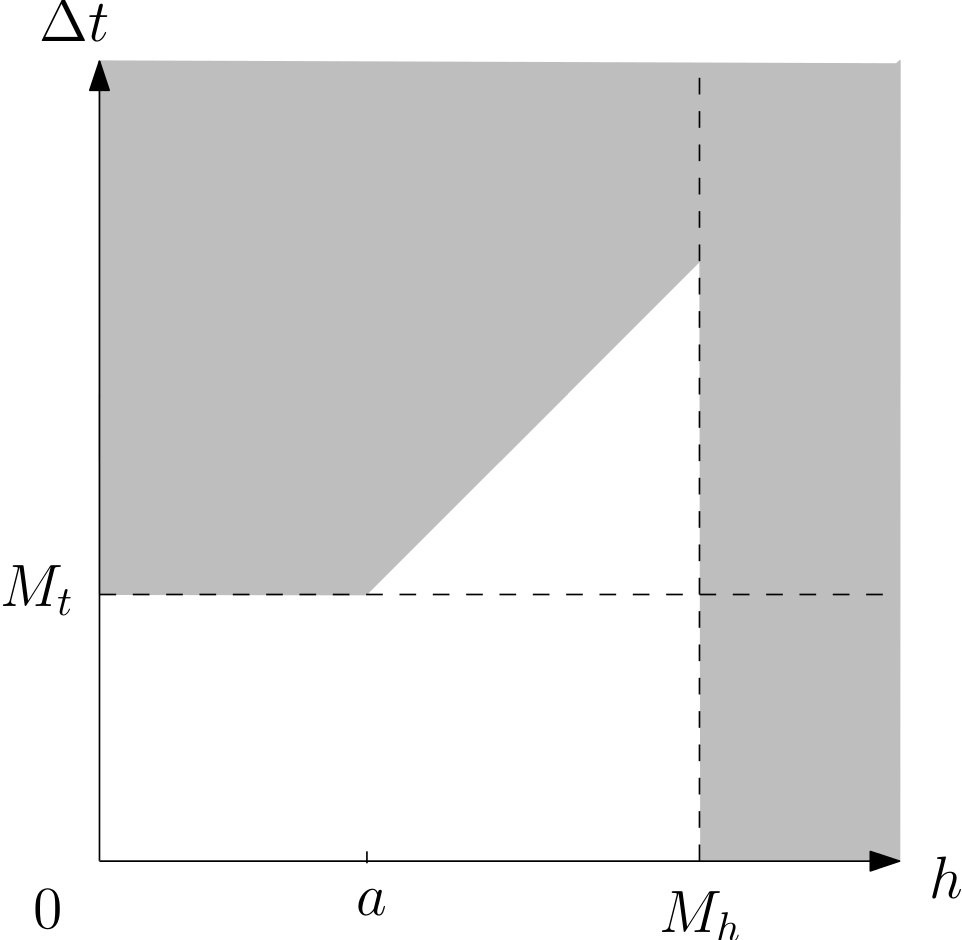
Figure 1: Stability region of a notional quasi-unconditionally stable method. The white region is the set of $(h,\Delta t)$ pairs for which the method is stable. Notice that outside of the quasi-unconditional stability rectangle $(0,M_{h})\times(0,M_{t})$, the present hypothetical method is stable for time steps satisfying the conditions $\Delta t<\min\{h,M_{h}\}$; other types of CFL-like conditions do, of course, occur commonly in practice. Thus, in particular, quasi-unconditional stability does not exclude the possibility of stability outside the rectangle $(0,M_{h})\times(0,M_{t})$.

In lieu of a full stability analysis for the main problem under consideration (the fully non-linear compressible Navier-Stokes equations, for which stability analyses are not available for any of the various extant algorithms), in support of the stability behavior observed in our numerical experiments we present rigorous stability results for simpler related problems. In particular, Section 4 establishes the unconditional stability of the Fourier-based BDF2-ADI scheme for linear constant coefficient hyperbolic and parabolic equations in two spatial dimensions. Section 5, in turn, shows that quasi-unconditional stability takes place for Fourier-spectral BDF methods of order $s$ ($2\leq s\leq 6$, without ADI) for the advection-diffusion equation in one- and two-dimensional space, and Section 6 presents numerical tests that demonstrate quasi-unconditional stability for the full compressible Navier-Stokes equations.

Remark 2.

In general, the stability of a PDE solver can be ensured provided relevant discrete operators are power bounded [18]. The von Neumann criterion provides a necessary but not sufficient condition for the power-boundedness of solution operators. If the discrete operators are non-normal, then stability analysis requires application of the Kreiss matrix theorem [10, p. 177]. In particular, it is known [18, 19] that certain discretizations and numerical boundary conditions can give rise to non-normal families of solution operators that are not power-bounded (and unstable) even though the underlying problem is linear with constant coefficients and all eigenvalues are inside the unit disk. (An operator $P$ with adjoint $P^{*}$ is normal if $P^{*}P=PP^{*}$.) In our Fourier-spectral context, however, all operators are normal (which follows from the fact that the first derivative operators are skew-Hermitian, the second derivative operators are Hermitian, and all derivative operators commute) and consequently the von Neumann criterion is both necessary and sufficient (cf. [11, p. 189]).

4 Unconditional stability for BDF2-ADI: periodic linear case

In this section the energy method is used to establish the unconditional stability of the BDF2-ADI scheme for the constant coefficient hyperbolic and parabolic equations with periodic boundary conditions under a Fourier collocation spatial approximation (Sections 4.3 and 4.4). In the case of the parabolic equation, further, an essentially identical argument is used in Section 4.5 to establish the corresponding unconditional stability result for the Legendre polynomial spectral collocation method with (non-periodic) homogeneous boundary conditions. Unfortunately, as discussed in that section, such a direct extension to the non-periodic case has not been obtained for the hyperbolic equation.

4.1 Preliminary definitions

We consider the domain

$$\Omega=[0,2\pi)\times[0,2\pi)$$ (10)

which we discretize on the basis of an odd number $N+1$ of discretization points ($N$ even, for definiteness) in both the $x$ and $y$ directions ($x_{j}=2\pi j/(N+1)$ and $y_{k}=2\pi k/(N+1)$, $0\leq j,k\leq N$), which gives rise to the grid

$$\{(x_{j},y_{k}):0\leq j,k\leq N\}.$$ (11)

(The restriction to even values of $N$, which is introduced for notational simplicity, allows us to avoid changes in the form of the summation limits in the Fourier series (14). Similarly, our use of equal numbers of points in the $x$ and $y$ directions simplifies the presentation somewhat. But, clearly, extensions of our constructions that allow for odd values of $N$ as well as unequal numbers of points in the $x$ and $y$ direction are straightforward.)

For (complex valued) grid functions

$$f=\{f_{jk}\}\text{ and }g=\{g_{jk}\},\quad 0\leq j,k\leq N$$ (12)

we define the discrete inner product and norm

$$(f,g)=\frac{1}{(N+1)^{2}}\sum\limits_{j,k}f_{jk}\bar{g}_{jk}$$ (13)

$$|f|=\sqrt{(f,f)}.$$

Each grid function $f$ as in (12) is can be associated to a trigonometric interpolant $f_{N}(x,y)$ ($f_{N}(x_{j},y_{k})=f_{jk}$) which is given by

$$f_{N}(x,y)=\sum_{|j|,|k|\leq\frac{N}{2}}\widehat{f}_{jk}e^{i(jx+ky)}$$ (14)

where

$$\widehat{f}_{jk}=\frac{1}{(N+1)^{2}}\sum\limits_{j,k}f_{jk}e^{-i(jx_{j}+ky_{k})}.$$

Note that the inner product (13) coincides with the trapezoidal quadrature rule applied to the grid functions $f$ and $g$ over the underlying domain $[0,2\pi)\times[0,2\pi)$. Since the trapezoidal rule is exact for all truncated Fourier series containing exponentials of the form $e^{-i(jx+ky)}$ with $-N\leq j,k\leq N$, it follows that the discrete inner product (13) equals the integral inner product of the corresponding trigonometric interpolants—i.e.

$$(f,g)=\frac{1}{(2\pi)^{2}}\int_{0}^{2\pi}\int_{0}^{2\pi}f_{N}(x,y)\bar{g}_{N}(x,y)\,dx\,dy.$$ (15)

In order to discretize solutions of PDEs we utilize time sequences of grid functions $u=\{u^{n}:n\geq 0\}$, where, for each $n$, $u^{n}=\{u^{n}_{jk}\}$ is a grid function such as those displayed in equation (12). For such time series the scalar product (13) at fixed $n$ can be used to produce a time series of scalar products: the inner product of two time series of grid functions $u=\{u^{n}:n\geq 0\}$ and $v=\{v^{n}:n\geq 0\}$ is thus a time series of complex numbers:

$$(u,v)=\{(u^{n},v^{n}):n\geq 0\}.$$

4.2 Discrete spatial and temporal operators

In order to discretize PDEs we use discrete spatial and temporal differentiation operators that act on grid functions and time-series, respectively.

We consider spatial differentiation first: the Fourier $x$-derivative operator $\delta_{x}$ applied to a grid function $f$, for example, is defined as the grid function $\delta_{x}f$ whose $jk$ value equals the value of the derivative of the interpolant $f_{N}$ at the point $(x_{j},y_{k})$:

$$(\delta_{x}f)_{jk}=\frac{\partial}{\partial x}f_{N}(x_{j},y_{k}).$$ (16)

The operators $\delta_{xx}$, $\delta_{y}$, $\delta_{yy}$, $\delta_{xy}=\delta_{x}\delta_{y}=\delta_{y}\delta_{x}$ etc. are defined similarly.

Using the exactness relation (15) and integration by parts together with the periodicity of the domain, it follows that the first derivative operators $\delta_{x}$ and $\delta_{y}$ are skew-Hermitian and the second derivative operators $\delta_{xx}$, $\delta_{yy}$ are Hermitian:

$$(\delta_{x}f,g)=-(f,\delta_{x}g),\;\;(\delta_{y}f,g)=-(f,\delta_{y}g),\;\;(\delta_{xx}f,g)=(f,\delta_{xx}g),\;\;(\delta_{yy}f,g)=(f,\delta_{yy}g).$$ (17)

Certain temporal differentiation and extrapolation operators we use, in turn, produce a new time series for a given time series—for both numerical time series as well as time series of grid functions. These operators include the regular first and second order finite difference operators $D$ and $D^{2}$, the three-point backward difference operator $\widehat{D}$ that is inherent in the BDF2 algorithm, as well as the second order accurate extrapolation operator “$\sim$”:

$$(Du)^{n} =u^{n}-u^{n-1}\quad n\geq 1$$ (18)

$$(D^{2}u)^{n} =(Du)^{n}-(Du)^{n-1}=u^{n}-2u^{n-1}+u^{n-2}\quad n\geq 2$$ (19)

$$(\widehat{D}u)^{n} =\frac{3}{2}u^{n}-2u^{n-1}+\frac{1}{2}u^{n-2}\quad n\geq 2$$ (20)

$$\widetilde{u}^{n+1} =2u^{n}-u^{n-1}\quad n\geq 1.$$ (21)

Note that the members of the time series $\widehat{D}u$ can also be expressed in the forms

$$(\widehat{D}u)^{n} =D\left(u^{n}+\frac{1}{2}(Du)^{n}\right)$$ (22)

$$=\frac{1}{2}((Du)^{n}+(D\widetilde{u})^{n+1})$$ (23)

$$=\frac{3}{2}(Du)^{n}-\frac{1}{2}(Du)^{n-1}.$$ (24)

In what follows we make frequent use of the finite difference product rule for two time series $u$ and $v$:

$$u\,Dv=D(uv)-v\,Du+(Du)\,(Dv).$$ (25)

An immediate consequence of (25), which will also prove useful, concerns the real part of scalar products of the form $(Du,P\,u)$ where $P$ is an operator which is self-adjoint with respect to the discrete inner product (13) and which commutes with $D$. For such operators we have the identity

$$\Re(Du,P\,u)=\frac{1}{2}D(u,P\,u)+\frac{1}{2}(Du,P\,Du)$$ (26)

which follows easily from the relations

$$(Du,P\,u) =D(u,P\,u)-(u,DP\,u)+(Du,DP\,u)$$

$$=D(u,P\,u)-(P\,u,Du)+(Du,P\,Du)$$

$$=D(u,P\,u)-\overline{(Du,P\,u)}+(Du,P\,Du).$$

4.3 Periodic BDF2-ADI stability: hyperbolic equation

This section establishes the unconditional stability of the BDF2-ADI method for the constant-coefficient advection equation

$$U_{t}+\alpha U_{x}+\beta U_{y}=0$$ (27)

in the domain (10), with real constants $\alpha$ and $\beta$, and subject to periodic boundary conditions. The BDF2-ADI scheme for the advection equation can be obtained easily by adapting the corresponding form (2) of the BDF2-ADI scheme for the pressure-free momentum equation. Indeed, using the Fourier collocation approximation described in the previous two sections, letting $u$ denote the discrete approximation of the solution $U$, and noting that, in the present context the necessary extrapolated term $\mathbf{\widetilde{u}}_{s-1}^{n+1}$ in equation (2) equals $u^{n}$, the factored form of our BDF2-ADI algorithm for equation (27) is given by

$$(I+b\Delta t\alpha\delta_{x})(I+b\Delta t\beta\delta_{y})u^{n+1}=a_{0}u^{n}+a_{1}u^{n-1}+\alpha\beta(b\Delta t)^{2}\delta_{x}\delta_{y}u^{n}.$$ (28)

Before proceeding to our stability result we derive a more convenient (equivalent) form for equation (28): using the numerical values $a_{0}=4/3$, $a_{1}=-1/3$, and $b=2/3$ of the BDF2 coefficients (see e.g. [14, Ch. 3.12] or Part I), the manipulations

$$0 =(I+b\Delta t\alpha\delta_{x})(I+b\Delta t\beta\delta_{y})u^{n+1}-a_{0}u^{n}-a_{1}u^{n-1}-\alpha\beta(b\Delta t)^{2}\delta_{x}\delta_{y}u^{n}$$

$$=u^{n+1}-a_{0}u^{n}-a_{1}u^{n-1}+b\Delta t\alpha\delta_{x}u^{n+1}+b\Delta t\beta\delta_{y}u^{n+1}+\alpha\beta(b\Delta t)^{2}\delta_{x}\delta_{y}(u^{n+1}-u^{n})$$

$$=\frac{1}{b}(u^{n+1}-a_{0}u^{n}-a_{1}u^{n-1})+\Delta t\alpha\delta_{x}u^{n+1}+\Delta t\beta\delta_{y}u^{n+1}+b\alpha\beta(\Delta t)^{2}\delta_{x}\delta_{y}(u^{n+1}-u^{n})$$

reduce equation (28) to the form

$$\widehat{D}u+A\,u+B\,u+bAB\,Du=0,$$ (29)

where $b=2/3$, $A=\alpha\Delta t\delta_{x}$ and $B=\beta\Delta t\delta_{y}$.

We are now ready to establish an energy stability estimate for the BDF2-ADI equation (28).

Theorem 1.

The solution $u$ of (28) with initial conditions $u^{0}$ and $u^{1}$ satisfies

$$|u^{n}|^{2}+|\widetilde{u}^{n+1}|^{2}+\frac{2}{3}\left(|Au^{n}|^{2}+|Bu^{n}|^{2}+\sum_{m=2}^{n}|(D^{2}u)^{m}|^{2}\right)\leq M$$

for all $n\geq 2$, where

$$M=|u^{1}|^{2}+|\widetilde{u}^{2}|^{2}+\frac{2}{3}(|Au^{1}|^{2}+|Bu^{1}|^{2}).$$

In particular, the scheme is unconditionally stable in the sense that a bound of the form given in equation (9) is satisfied.

Proof.

Taking the inner product of equation (29) with $u$ we obtain

$$0 =(u,\widehat{D}u) +(u,A\,u) +(u,B\,u) +b(u,AB\,Du)$$ (30)

$$=(\mathit{I}) +(\mathit{II}) +(\mathit{III}) +(\mathit{IV}),$$

where $(I)=(u,\widehat{D}u)$, $(\mathit{II})=(u,A\,u)$, etc. Our goal is to express the real part of the right-hand side in (30) as a sum of non-negative terms and telescoping terms of the form $Df$ for some non-negative numerical time series $f$. To that end, we consider the terms $(I)$ through $(\mathit{IV})$ in turn.

$(\mathit{I})$:

Using the expression (23) for $\widehat{D}u$ we obtain

$$(I)=\frac{1}{2}(u,Du)+\frac{1}{2}(u,D\widetilde{w}),$$ (31)

where $\widetilde{w}$ denotes the time series obtained by shifting $\widetilde{u}$ forwards by one time step:

$$\widetilde{w}=\{\widetilde{w}^{n}=\widetilde{u}^{n+1}:n\geq 1\}.$$ (32)

To re-express (31) we first note that for any two grid functions $a$ and $b$ we have the relation

$$|a-b|^{2}=|a|^{2}+|b|^{2}-2\Re(a,b)$$

$$\implies \Re(a,b)=\frac{1}{2}(|a|^{2}+|b|^{2}-|a-b|^{2}).$$

Therefore, for any time series $g$ we have

$$\Re(u,Dg)^{n} =\Re(u^{n},g^{n})-\Re(u^{n},g^{n-1})$$

$$=\frac{1}{2}(|u^{n}|^{2}+|g^{n}|^{2}-|u^{n}-g^{n}|^{2})-\frac{1}{2}(|u^{n}|^{2}+|g^{n-1}|^{2}-|u^{n}-g^{n-1}|^{2})$$

$$=\frac{1}{2}(D|g^{n}|^{2}-|u^{n}-g^{n}|^{2}+|u^{n}-g^{n-1}|^{2}).$$ (33)

Letting $g=u$ and $g=\widetilde{w}$ in (33) we obtain

$$\Re(u,Du)=\frac{1}{2}(D|u|^{2}+|Du|^{2})\\$$ (34)

and

$$\Re(u,D\widetilde{w})=\frac{1}{2}(D|\widetilde{w}|^{2}-|Du|^{2}+|D^{2}u|^{2}).$$ (35)

Replacing (34) and (35) in (31) we obtain

$$\Re(\mathit{I})=\frac{1}{4}D(|u|^{2}+|\widetilde{w}|^{2})+\frac{1}{4}|D^{2}u|^{2}.$$ (36)

Notice that this equation expresses $\Re(\mathit{I})$ as the sum of a telescoping term and a positive term, as desired.

$(\mathit{II})$ and $(\mathit{III})$:

The operator $A$ is clearly skew-Hermitian since $\delta_{x}$ is. Therefore

$$(\mathit{II})=(u,Au)=-(Au,u)=-\overline{(u,Au)}$$

$$\implies \Re(\mathit{II})=0.$$ (37)

The relation

$$\Re(\mathit{III})=\Re(u,Bu)=0$$ (38)

follows similarly, of course.

$(\mathit{IV})$:

Lemma 1 below tells us that

$$\Re(u,AB\,Du)\geq\frac{1}{4}D\left(|Au|^{2}+|Bu|^{2}\right)-\frac{1}{8}|D^{2}u|^{2}.$$ (39)

Substituting (36), (37), (38), and (39) into equation (30) (recalling $b=2/3$) and taking the real part we obtain

$$0\geq\frac{1}{4}D\left(|u|^{2}+|\widetilde{w}|^{2}\right)+\frac{1}{6}\left(|Au|^{2}+|Bu|^{2}+|D^{2}u|^{2}\right),$$ (40)

which is the sum of a telescoping term and a non-negative term. Multiplying by the number four and summing the elements of the above numerical time series from $m=2$ to $n$ completes the proof of the theorem. ∎

The following lemma concerns the bound (39) used in Theorem 1.

Lemma 1.

Any solution of equation (29) satisfies (39).

Proof.

Taking the inner product of (29) with $A\,Du$ (using the form (22) of $\widehat{D}u$) we obtain

$$0=(Du,A\,Du)+\frac{1}{2}(D^{2}u,A\,Du)+(A\,u,A\,Du)+(B\,u,A\,Du)+b(AB\,Du,A\,Du).$$ (41)

Since $A$ and $B$ commute and since $B$ is skew-Hermitian (equation (17)) we have

$$(B\,u,A\,Du) =-(u,AB\,Du)$$

for the next-to-last term in (41). Therefore, equation (41) can be re-expressed in the form

$$(u,AB\,Du) =(Du,A\,Du) +\frac{1}{2}(D^{2}u,A\,Du) +(A\,u,A\,Du) +b(AB\,Du,A\,Du)$$ (42)

$$=(\mathit{I}) +(\mathit{II}) +(\mathit{III}) +(\mathit{IV}).$$

We consider each term in (42) in turn.

$(\mathit{I})$:

Since $A$ is skew-Hermitian it follows that the real part of this term vanishes:

$$(\mathit{I})=(Du,A\,Du)=-(A\,Du,Du)=-\overline{(Du,A\,Du)}=-\overline{(\mathit{I})}$$

$$\implies \Re(\mathit{I})=0.$$ (43)

$(\mathit{II})$:

Using Young’s inequality

$$ab\leq\frac{r}{2}a^{2}+\frac{1}{2r}b^{2}$$ (44)

(which, as is easily checked, is valid for all real numbers $a$ and $b$ and for all $r>0$) together with the Cauchy-Schwarz inequality we obtain

$$\Re(\mathit{II}) =\frac{1}{2}\Re(D^{2}u,A\,Du)$$

$$\geq-\frac{1}{2}|(D^{2}u,A\,Du)|$$

$$\geq-\frac{1}{2}|D^{2}u|\,|A\,Du|$$

$$\geq-\frac{1}{2}(\frac{1}{4}|D^{2}u|^{2}+|A\,Du|^{2})$$

$$=-\frac{1}{8}|D^{2}u|^{2}-\frac{1}{2}|A\,Du|^{2}.$$ (45)

$(\mathit{III})$:

By the finite-difference product rule (25) we obtain

$$\mathit{(III)} =(Au,D(Au))$$

$$=D(Au,Au)-(DAu,Au)+(DAu,DAu)$$

$$=D|Au|^{2}-\overline{(III)}+|A\,Du|^{2}$$

$$\implies \Re(III) =\frac{1}{2}D|Au|^{2}+\frac{1}{2}|A\,Du|^{2}.$$ (46)

$(\mathit{IV})$:

Again using the fact that $B$ is skew-Hermitian and commutes with $A$ it follows that

$$(\mathit{IV})=b(BA\,Du,A\,Du)=-b(A\,Du,BA\,Du)=-\overline{\mathit{(IV)}}$$

$$\implies \Re(\mathit{IV})=0.$$ (47)

Combining the real parts of equations (42), (43), (45), (46) and (47) we obtain

$$\Re(u,AB\,Du)\geq\frac{1}{2}D|Au|^{2}-\frac{1}{8}|D^{2}u|^{2}.$$ (48)

An analogous result can be obtained by taking the inner product of equation (29) with $B\,Du$ instead of $A\,Du$ and following the same steps used to arrive at equation (48). The result is

$$\Re(u,AB\,Du)\geq\frac{1}{2}D|Bu|^{2}-\frac{1}{8}|D^{2}u|^{2}.$$ (49)

The lemma now follows by averaging equations (48) and (49). ∎

4.4 Fourier-based BDF2-ADI stability: parabolic equation

This section establishes the unconditional stability of the BDF2-ADI method for the constant-coefficient parabolic equation

$$U_{t}=\alpha\,U_{xx}+\beta\,U_{yy}+\gamma\,U_{xy}.$$ (50)

Notice the inclusion of the mixed derivative term, which is treated explicitly using temporal extrapolation in the BDF-ADI algorithm. Theorem 2 in this section proves, in particular, that extrapolation of the mixed derivative does not compromise the unconditional stability of the method.

The parabolicity conditions $\alpha>0$, $\beta>0$ and

$$\gamma^{2}\leq 4\alpha\beta,$$ (51)

which are assumed throughout this section, ensure that

$$\int_{0}^{2\pi}\int_{0}^{2\pi}f\left(\alpha\,f_{xx}+\beta\,f_{yy}+\gamma\,f_{xy}\right)\,dx\,dy\leq 0$$ (52)

for any twice continuously differentiable bi-periodic function $f$ defined in the domain (10)—as can be established easily by integration by parts and completion of the square in the sum $\alpha(f_{x})^{2}+\gamma f_{x}f_{y}$ together with some simple manipulations. In preparation for the stability proof that is put forth below in this section, in what follows we present a few preliminaries concerning the BDF2-ADI algorithm for equation (50).

We first note that a calculation similar to that leading to equation (29) shows that the Fourier-based BDF2-ADI scheme for (50) can be expressed in the form

$$\widehat{D}u-\Delta t(\alpha\,\delta_{xx}+\beta\,\delta_{yy}u+\gamma\,\delta_{x}\delta_{y})u+\Delta t\,\gamma\,\delta_{x}\delta_{y}\,D^{2}u+b(\Delta t)^{2}\alpha\beta\,\delta_{xx}\delta_{yy}\,Du=0.$$ (53)

Letting

$$A=-\Delta t\,\alpha\,\delta_{xx},$$

$$B=-\Delta t\,\beta\,\delta_{yy},$$

$$F=-\Delta t\,\gamma\,\delta_{x}\delta_{y},$$

$$L=A+B+F,$$

equation (53) becomes

$$\widehat{D}u+Lu-F\,D^{2}u+bAB\,Du=0.$$ (54)

Note that the operators $A$ and $B$ above do not coincide with the corresponding $A$ and $B$ operators in Section 4.3.

In view of the exactness relation (15) together with the Fourier differentiation operators (cf. (16)), it follows that $A$, $B$, $AB$ and $L$ are positive semidefinite operators. Indeed, in view of equation (52), for example, we have

$$(u,L\,u) =-\frac{\Delta t}{(2\pi)^{2}}\int_{0}^{2\pi}\int_{0}^{2\pi}u_{N}\,\left(\alpha(u_{N})_{xx}+\beta(u_{N})_{yy}+\gamma(u_{N})_{xy}\right)\,dx\,dy$$

$$\geq 0;$$ (55)

similar relations for $A$, $B$ and $AB$ follow directly by integration by parts.

Finally we present yet another consequence of the parabolicity condition (51) which will prove useful: for any grid function $g$ we have

$$|Fg|^{2}=\gamma^{2}\,(\Delta t)^{2}(\delta_{x}\delta_{y}g,\delta_{x}\delta_{y}g)\leq 4\alpha\beta(\Delta t)^{2}(g,\delta_{x}^{2}\delta_{y}^{2}g)=4(g,ABg).$$ (56)

Thus, defining the seminorm

$$|u|_{P}=\sqrt{(u,Pu)}$$ (57)

for a given positive semidefinite operator $P$ and using $P=AB$ we obtain

$$|Fg|^{2}\leq 4|g|^{2}_{AB}.$$ (58)

The following theorem can now be established.

Theorem 2.

The solution $u$ of the Fourier-based BDF2-ADI scheme  (53) for equation (50) with initial conditions $u^{0}$, $u^{1}$ satisfies

$$\frac{1}{4}|u^{n}|^{2}+\frac{1}{4}|\widetilde{u}^{n+1}|^{2}+\frac{1}{3}|(Du)^{n}|_{AB}^{2}+\frac{1}{4}\sum_{m=1}^{n}|D^{2}u|^{2}+\sum_{m=1}^{n}|u^{n}|_{L}^{2}\leq M$$

for $n\geq 2$, where

$$M= \frac{1}{4}|u^{1}|^{2}+\frac{1}{4}|\widetilde{u}^{2}|^{2}+\frac{1}{3}|u^{1}|_{AB}^{2}+3|u^{1}|_{L}-\Re(u^{1},F\,(Du)^{1})$$

$${}+3|(Du)^{1}|^{2}+\frac{3}{2}\left(|(Du)^{1}|_{A}^{2}+|(Du)^{1}|_{B}^{2}\right)+\frac{1}{3}|(Du)^{1}|_{AB}^{2}.$$

In particular, the scheme is unconditionally stable in the sense that a bound of the form given in equation (9) is satisfied.

Proof.

Taking the inner product of (54) with $u$ we obtain

$$0 =(u,\widehat{D}u) +(u,Lu) -(u,F\,D^{2}u) +b(u,AB\,Du)$$ (59)

$$=(I) +(\mathit{II}) +(\mathit{III}) +(\mathit{IV}),$$

where $(I)=(u,\widehat{D}u)$, $(\mathit{II})=(u,Lu)$, etc. As in Theorem 1, we re-express the above equation using telescoping and non-negative terms to obtain the desired energy bound.

The term $(I)$ already occurs in the proof of Theorem 1; there we obtained the relation

$$\Re(\mathit{I})=\frac{1}{4}D(|u|^{2}+|\widetilde{w}|^{2})+\frac{1}{4}|D^{2}u|^{2},$$ (60)

where $\widetilde{w}$ is defined in (32). The term $(\mathit{II})=|u|_{L}^{2}$, in turn, is non-negative (see equation (4.4)) and thus requires no further treatment. The remaining two terms are considered in what follows.

$(\mathit{III})$:

This term presents the most difficulty, since $F$ is not positive semi-definite. In what follows the term ($\mathit{III}$) is re-expressed as a a sum of two quantities, the first one of which can be combined with a corresponding term arising from the quantity $\mathit{(IV)}$ to produce a telescoping term, and the second of which will be addressed towards the end of the proof by utilizing Lemma 2 below.

Let $v$ denote the time series obtained by shifting $u$ backwards by one time step:

$$v=\{v^{n}=u^{n-1}:n\geq 1\};$$ (61)

clearly we have

$$Du=u-v\quad\mbox{and}\quad D^{2}u=Du-Dv.$$ (62)

Thus, using the finite difference product rule (25) and the second relation in (62) we obtain

$$(\mathit{III}) =-(u,F\,D(Du))=-(u,D\,F(Du))$$

$$=-D(u,F\,Du)+(Du,F\,Du)-(Du,F\,D^{2}u)$$

$$=-D(u,F\,Du)+(Du,F\,Dv).$$

Applying the Cauchy-Schwarz inequality and Young’s inequality (44) with $r=6$ together with (58) we obtain

$$\Re(\mathit{III}) \geq-D\Re(u,F\,Du)-|Du|\,|F\,Dv|$$

$$\geq-D\Re(u,F\,Du)-3|Du|^{2}-\frac{1}{12}|F\,Dv|^{2}$$

$$\geq-D\Re(u,F\,Du)-3|Du|^{2}-\frac{1}{3}|Dv|_{AB}^{2}.$$ (63)

The last term in the above inequality will be combined with an associated expression in $(\mathit{IV})$ below to produce a telescoping term.

$(\mathit{IV})$:

Using the finite difference product rule (26) together with the fact that $AB$ is a Hermitian positive semi-definite operator we obtain

$$\Re(\mathit{IV}) =\frac{2}{3}\Re(u,AB\,Du)=\frac{2}{3}\Re(Du,ABu)$$

$$=\frac{1}{3}D(u,AB\,u)+\frac{1}{3}(Du,AB\,Du)$$

$$=\frac{1}{3}D|u|_{AB}^{2}+\frac{1}{3}|Du|_{AB}^{2}$$ (64)

(see equation (57)). Substituting (60), (63) and (64) into equation (59), recalling equation (32) and taking real parts, we obtain

$$0\geq \frac{1}{4}D(|u|^{2}+|\widetilde{w}|^{2})+\frac{1}{4}|D^{2}u|^{2}+|u|_{L}^{2}-D\Re(u,F\,Du)-3|Du|^{2}$$

$${}+\frac{1}{3}(|Du|_{AB}^{2}-|Dv|_{AB}^{2})+\frac{1}{3}D|u|_{AB}^{2}$$

$$= D\left(\frac{1}{4}|u|^{2}+\frac{1}{4}|\widetilde{w}|^{2}+\frac{1}{3}|u|_{AB}^{2}+\frac{1}{3}|Du|_{AB}^{2}-\Re(u,F\,Du)\right)$$

$${}+|u|_{L}^{2}+\frac{1}{4}|D^{2}u|^{2}-3|Du|^{2}.$$ (65)

Adding the time series (4.4) from $m=2$ to $n$ and using the identity $\widetilde{w}^{n}=\widetilde{u}^{n+1}$ we obtain

$$M_{1} \geq \frac{1}{4}|u^{n}|^{2}+\frac{1}{4}|\widetilde{u}^{n+1}|^{2}+\,\frac{1}{3}|u^{n}|_{AB}^{2}+\frac{1}{3}|(Du)^{n}|_{AB}^{2}+\sum_{m=2}^{n}|u^{n}|_{L}^{2}$$ (66)

$$+\frac{1}{4}\sum_{m=2}^{n}|(D^{2}u)^{n}|^{2}-3\sum_{m=2}^{n}|(Du)^{m}|^{2}-\Re(u^{n},F\,(Du)^{n})$$

where

$$M_{1}=\frac{1}{4}|u^{1}|^{2}+\frac{1}{4}|\widetilde{u}^{2}|^{2}+\frac{1}{3}|u^{1}|_{AB}^{2}+\frac{1}{3}|(Du)^{1}|_{AB}^{2}-\Re(u^{1},F\,(Du)^{1}).$$

Using Cauchy-Schwarz and Young’s inequalities along with the parabolicity relation (58) and the fact that $F$ is a Hermitian operator, the last term $-\Re(u^{n},F\,(Du)^{n})$ in (66) is itself estimated as follows:

$$-\Re(u^{n},F\,(Du)^{n}) = -\Re(F\,u^{n},(Du)^{n})$$

$$\geq -|F\,u^{n}||(Du)^{n}|$$

$$\geq -\frac{1}{12}|F\,u^{n}|^{2}-3|(Du)^{n}|^{2}$$

$$\geq -\frac{1}{3}|u^{n}|_{AB}^{2}-3|(Du)^{n}|^{2}.$$

Equation (66) may thus be re-expressed in the form

$$\frac{1}{4}|u^{n}|^{2} + \frac{1}{4}|\widetilde{u}^{n+1}|^{2}+\frac{1}{3}|(Du)^{n}|_{AB}^{2}+\sum_{m=2}^{n}|u^{n}|_{L}^{2}+\frac{1}{4}\sum_{m=2}^{n}|D^{2}u|^{2}$$ (67)

$$\leq M_{1}+3|(Du)^{n}|^{2}+3\sum_{m=2}^{n}|(Du)^{m}|^{2}.$$

Finally, applying Lemma 2 below to the last two terms on the right-hand side of equation (67) we obtain

$$3|(Du)^{n}|^{2}+3\sum_{m=2}^{n}|(Du)^{m}|^{2}\leq 3M_{2},$$

where the constant $M_{2}$ is given by equation (69) below, and the proof of the theorem is thus complete. ∎

The following lemma, which provides a bound on sums of squares of the temporal difference $Du$, is used in the proof of Theorem 2 above.

Lemma 2.

The solution $u$ of the Fourier-based BDF2-ADI scheme  (53) for equation (50) with initial conditions $u^{0}$, $u^{1}$ satisfies

$$|(Du)^{n}|^{2}+|u^{n}|^{2}_{L}+\frac{1}{2}\left(\,|(Du)^{n}|_{A}^{2}+|(Du)^{n}|_{B}^{2}\,\right)+\sum_{m=2}^{n}|(Du)^{m}|^{2}\leq M_{2}$$ (68)

for $n\geq 2$, where

$$M_{2}=|(Du)^{1}|^{2}+|u^{1}|^{2}_{L}+\frac{1}{2}\left(\,|(Du)^{1}|_{A}^{2}+|(Du)^{1}|_{B}^{2}\,\right).$$ (69)

Proof.

We start by taking the inner product of equation (54) with $Du$ to obtain

$$0 =(Du,\widehat{D}u) +(Du,Lu) -(Du,F\,D^{2}u) +b(Du,AB\,Du)$$ (70)

$$=(I) +(\mathit{II}) +(\mathit{III}) +(\mathit{IV}).$$

We now estimate each of the terms $(I)$ through $(\mathit{IV})$ in turn; as it will become apparent, the main challenge in this proof lies in the estimate of the term $(\mathit{III})$.

$(I)$:

Using (22) and the finite difference product rule (26), $(I)$ can be expressed in the form

$$\Re(I) =\Re(Du,Du+\frac{1}{2}D^{2}u)$$

$$=|Du|^{2}+\frac{1}{4}D|Du|^{2}+\frac{1}{4}|D^{2}u|^{2}.$$ (71)

$(\mathit{II})$:

Using equation (26) we obtain

$$\Re(\mathit{II})=\Re(Du,Lu)=\frac{1}{2}D(u,Lu)+\frac{1}{2}(Du,L\,Du).$$

Since $L=A+B+F$ we may write

$$\Re(\mathit{II})=\frac{1}{2}D|u|_{L}^{2}+\frac{1}{2}|Du|_{A+B}^{2}+\frac{1}{2}(Du,F\,Du).$$ (72)

The last term in this equation (which is a real number in view of the Hermitian character of the operator $F$) will be used below to cancel a corresponding term in our estimate of $(\mathit{III})$.

$(\mathit{III})$:

Using (61) together with the second equation in (62), $(\mathit{III})$ can be expressed in the form

$$(\mathit{III}) =-(Du,F\,D^{2}u)$$

$$=-\frac{1}{2}(Du,F\,Du)+\frac{1}{2}(Du,F\,Dv)-\frac{1}{2}(Du,F\,D^{2}u).$$ (73)

The first term on the right-hand side of (4.4) will be used to cancel the last term in (72). Hence it suffices to obtain bounds for the second and third terms on the right-hand side of equation (4.4).

To estimate the second term in (4.4) we consider the relation

$$\frac{1}{2}(Du,F\,Dv)=\frac{1}{2}\gamma\,\Delta t\,(Du,\delta_{x}\delta_{y}Dv)=-\frac{\gamma}{4}\,\Delta t\,(\delta_{x}\,Du,\delta_{y}\,Dv)-\frac{\gamma}{4}\,\Delta t\,(\delta_{y}\,Du,\delta_{x}\,Dv),$$ (74)

which follows from the fact that $\delta_{x}$ and $\delta_{y}$ are skew-Hermitian operators. Taking real parts and applying the Cauchy-Schwarz and Young inequalities together with the parabolicity condition (51) we obtain

$$\frac{1}{2}\Re(Du,F\,Dv)\geq -\frac{\sqrt{\alpha\beta}}{2}\,\Delta t\,\left(\frac{1}{2}\sqrt{\frac{\alpha}{\beta}}\,|\delta_{x}\,Du|^{2}+\frac{1}{2}\sqrt{\frac{\beta}{\alpha}}\,|\delta_{y}\,Dv|^{2}\right)$$

$${}-\frac{\sqrt{\alpha\beta}}{2}\,\Delta t\,\left(\frac{1}{2}\sqrt{\frac{\beta}{\alpha}}\,|\delta_{y}\,Du|^{2}+\frac{1}{2}\sqrt{\frac{\alpha}{\beta}}\,|\delta_{x}\,Dv|^{2}\right)$$

$$= -\frac{1}{4}\Delta t\,(\alpha\,|\delta_{x}\,Du|^{2}+\beta\,|\delta_{y}\,Du|^{2})-\frac{1}{4}\Delta t\,(\alpha\,|\delta_{x}\,Dv|^{2}+\beta\,|\delta_{y}\,Dv|^{2})$$

$$= -\frac{1}{4}|Du|^{2}_{A+B}-\frac{1}{4}|Dv|^{2}_{A+B}.$$ (75)

To estimate third term in (4.4) we once again use the Cauchy-Schwarz and Young inequalities and we exploit the relation (58); we thus obtain

$$-\frac{1}{2}\Re(Du,F\,D^{2}u) =-\frac{1}{2}\Re(F\,Du,D^{2}u)$$

$$\geq-\frac{1}{6}|F\,Du|^{2}-\frac{3}{8}|D^{2}u|^{2}$$

$$\geq-\frac{2}{3}|Du|^{2}_{AB}-\frac{3}{8}|D^{2}u|^{2}.$$ (76)

Taking the real part of (4.4) and using equations (75) and (76) we obtain the relation

$$\Re(\mathit{III})\geq-\frac{1}{2}\Re(Du,F\,Du)-\frac{1}{4}|Du|^{2}_{A+B}-\frac{1}{4}|Dv|^{2}_{A+B}-\frac{2}{3}|Du|^{2}_{AB}-\frac{3}{8}|D^{2}u|^{2},$$ (77)

which, as shown below, can be combined with the estimates for $(I)$, $\mathit{(II)}$, and $\mathit{(IV)}$ to produce an overall estimate that consists solely of non-negative and telescoping terms—as desired.

$(\mathit{IV})$:

In view of (57) we see that $(\mathit{IV})$ coincides with the $P$-seminorm of $Du$ with $P=AB$,

$$\Re(\mathit{IV})=(\mathit{IV})=\frac{2}{3}|Du|^{2}_{AB}.$$ (78)

This term is non-negative and it therefore does not require further treatment.

To complete the proof of the lemma we take real parts in equation (70) and we substitute (71), (72), (77) and (78); the result is

$$0\geq |Du|^{2}+\frac{1}{4}D|Du|^{2}-\frac{1}{8}|D^{2}u|^{2}+\frac{1}{2}D|u|_{L}^{2}+\frac{1}{4}|Du|_{A+B}^{2}-\frac{1}{4}|Dv|^{2}_{A+B}$$

$$= |Du|^{2}-\frac{1}{8}|D^{2}u|^{2}+D\left(\frac{1}{4}|Du|^{2}+\frac{1}{2}|u|_{L}^{2}+\frac{1}{4}|Du|_{A+B}^{2}\right).$$ (79)

The first two terms on the right-hand-side can be bounded by expanding $|D^{2}u|^{2}$ and using Cauchy-Schwarz and Young’s inequalities to obtain

$$|Du|^{2}-\frac{1}{8}|D^{2}u|^{2} =|Du|^{2}-\frac{1}{8}|Du-Dv|^{2}$$ (80)

$$=|Du|^{2}-\frac{1}{8}(|Du|^{2}+|Dv|^{2})+\frac{1}{4}\Re(Du,Dv)$$ (81)

$$\geq|Du|^{2}-\frac{1}{8}(|Du|^{2}+|Dv|^{2})-\frac{1}{4}|Du||Dv|$$ (82)

$$\geq|Du|^{2}-\frac{1}{4}(|Du|^{2}+|Dv|^{2})$$ (83)

$$=\frac{1}{2}|Du|^{2}+\frac{1}{4}D|Du|^{2}.$$ (84)

Substituting this result into (79), we obtain

$$0\geq \frac{1}{2}|Du|^{2}+D\left(\frac{1}{2}|Du|^{2}+\frac{1}{2}|u|_{L}^{2}+\frac{1}{4}|Du|_{A+B}^{2}\right),$$ (85)

which, as needed, is expressed as a sum of non-negative and telescoping terms. Adding the time-series (85) from $m=2$ to $n$ yields the desired equation (68), and the proof is thus complete. ∎

Remark 3.

It is interesting to point out that Lemma 2 by itself implies a weak stability result that follows from equation (68) and the Cauchy-Schwarz inequality:

$$|u^{n}| =|u^{1}+\sum_{m=2}^{n}(Du)^{m}|$$

$$\leq|u^{1}|+\sum_{m=2}^{n}|(Du)^{m}|$$

$$\leq|u^{1}|+\left(n\sum_{m=2}^{n}|(Du)^{m}|^{2}\right)^{\frac{1}{2}}$$

$$\leq|u^{1}|+\sqrt{nM_{2}},$$ (86)

Theorem 2 provides a much tighter energy estimate than (86), of course.

4.5 Non-periodic (Legendre based) BDF2-ADI stability: parabolic equation

The stability result provided in the previous section for the parabolic equation with periodic boundary conditions can easily be extended to a non-periodic setting using a spatial approximation based on use of Legendre polynomials. Here we provide the main necessary elements to produce the extensions of the proofs. Background on the polynomial collocation methods may be found e.g. in [13].

Under Legendre collocation we discretize the domain $\Omega=[-1,1]\times[-1,1]$ by means of the $N+1$ Legendre Gauss-Lobatto quadrature nodes $x_{j}=y_{j}$ ($j=0,\dots,N$) in each one of the coordinate directions, which defines the grid $\{(x_{j},y_{k}):0\leq j,k\leq N\}$ (with $x_{0}=y_{0}=-1$ and $x_{N}=y_{N}=1$). For real-valued grid functions $f=\{f_{jk}\}$ and $g=\{g_{jk}\}$ we use the inner product

$$(f,g)=\sum_{j=0}^{N}\sum_{k=0}^{N}w_{j}w_{k}f_{jk}g_{jk},$$ (87)

where $w_{\ell}$ ($0\leq\ell\leq N$) are the Legendre Gauss-Lobatto quadrature weights. The interpolant $f_{N}$ of a grid function $f$ is a linear combination of the form

$$f_{N}(x,y)=\sum_{j=0}^{N}\sum_{k=0}^{N}\widehat{f}_{jk}P_{j}(x)P_{k}(y).$$

of Legendre polynomials $P_{j}$, where $\widehat{f}_{jk}$ are the Legendre coefficients of $f_{N}$.

A certain exactness relation similar to the one we used in the Fourier case exists in the Legendre context as well. Namely, for grid functions $f$ and $g$ for which the product of the interpolants has polynomial degree $\leq 2N-1$ in the $x$ (resp. $y$) variable, the $j$ (resp. $k$) summation in the inner product (87) of the two grid functions is equal to the integral of the product of their corresponding polynomial interpolants with respect to $x$ (resp. $y$) [11, Sec. 5.2.1]—i.e.

$$(f,g)=\sum_{k=0}^{N}\int_{-1}^{1}f_{N}(x,y_{k})g_{N}(x,y_{k})\,dx,$$ (88a)

provided

$$\deg(f_{N}(x,y_{k})g_{N}(x,y_{k}))\leq 2N-1\text{ for all }0\leq k\leq N,$$

and

$$(f,g)=\sum_{j=0}^{N}\int_{-1}^{1}f_{N}(x_{j},y)g_{N}(x_{j},y)\,dy,$$ (88b)

provided

$$\deg(f_{N}(x_{j},y)g_{N}(x_{j},y))\leq 2N-1\text{ for all }0\leq j\leq N,$$

Thus, for example, defining the Legendre $x$-derivative operator $\delta_{x}$ as the derivative of the Legendre interpolant (cf. (16)) (with similar definitions for $\delta_{y}$, $\delta_{xx}$, $\delta_{yy}$ etc.), the exactness relation (88a) holds whenever one or both of the grid functions $f$ and $g$ is a Legendre $x$-derivative of a grid function $h=\{h_{jk}\}$, $0\leq j,k\leq N$.

A stability proof for the parabolic equation with zero Dirichlet boundary conditions,

$$U_{t}=\alpha\,U_{xx}+\beta\,U_{yy}+\gamma\,U_{xy}\text{ in }\Omega,\quad U=0\text{ on }\partial\Omega,$$

can now be obtained by reviewing and modifying slightly the strategy presented for the periodic case in Section 4.4. Indeed, the latter proof relies on the following properties of the spatial differentiation operators:

1. The discrete first and second derivative operators are skew-Hermitian and Hermitian, respectively.

2. The operators $A$, $B$, $L$ and $AB$ defined in Section 4.4 are positive semi-definite.

Both of these results were established using the exactness relation between the discrete and integral inner products together with vanishing boundary terms arising from integration by parts—which also hold in the present case since the exactness relations (88) are only required in the proof to convert inner products involving derivatives, so that the degree of polynomial interpolants will satisfy the requirements of the relations (88). Since all other aspects of the proofs in Section 4.4 are independent of the particular spatial discretization or boundary conditions used, we have the following theorem:

Theorem 3.

The stability estimate given in Theorem 2 also holds on the domain $[-1,1]\times[-1,1]$ with homogeneous boundary conditions using the Legendre Gauss-Lobatto collocation method, where the inner products and norms are taken to be the Legendre versions.

Remark 4.

Unfortunately, the stability proof cannot be extended directly to the non-periodic hyperbolic case. Indeed, since in this case only one boundary condition is specified in each spatial direction, not all boundary terms arising from integration by parts vanish—and, hence, the first derivative operators are generally not skew-Hermitian. See [9] for a discussion of spectral method stability proofs for hyperbolic problems.

5 Quasi-unconditional stability for higher-order non-ADI BDF methods: periodic advection-diffusion equation

5.1 Rectangular window of stability

This paper does not present stability proofs for the BDF-ADI methods of order higher than two. In order to provide some additional insights into the stability properties arising from the BDF strategy in the context of time-domain PDE solvers, this section investigates the stability of the BDF schemes of order $s\geq 2$—cf. Remark 2 as well as the last paragraph in Section 3—under periodic boundary conditions and Fourier discretizations. Because of Dahlquist’s second barrier [14, p. 243] the $s\geq 3$ schemes cannot be unconditionally stable for general (even linear) PDEs. However, we will rigorously establish that the BDF methods of order $s$ with $2\leq s\leq 6$ are quasi-unconditionally stable for the advection-diffusion equation—in the sense of Definition 1. (As shown in Section 4 further, the $s=2$ algorithms are indeed unconditionally stable, at least for certain linear PDE.)

To introduce the main ideas in our quasi-unconditional stability analysis for BDF-based schemes we consider first a Fourier-BDF scheme for the advection-diffusion equation in one spatial dimension with periodic boundary conditions:

$$U_{t}+\alpha U_{x}=\beta U_{xx},\quad x\in\mathbb{R},\quad t\geq 0,$$ (89)

$$U(x,0)=f(x),\quad U(x,t)=U(x+2\pi,t),$$

where $\beta>0$. Using the $N$-point Fourier discretization described in Sections 4.1 and 4.2, the resulting semi-discrete equation is given by

$$\frac{\partial}{\partial t}u=(-\alpha\,\delta_{x}+\beta\,\delta_{x}^{2})\,u.$$ (90)

As mentioned in Remark 2, the von Neumann criterion provides a necessary and sufficient stability condition for this problem: the order-$s$ scheme is stable if and only if the (complex!) eigenvalues of the spatial operator in the semi-discrete system (90) multiplied by $\Delta t$ lie within the region $R_{s}$ of absolute stability of the BDF method of order $s$. We will see that, for the present one-dimensional advection-diffusion problem, these eigenvalues lie on a parabola which does not vary with $N$. As is known [15, Sec. 7.6.1 and p. 174], further, the boundary of $R_{s}$ is given by the polar parametrization

$$z(\theta)=\frac{1}{b}\left(1-\sum_{j=0}^{s-1}a_{j}e^{-i(j+1)\theta}\right).$$ (91)

To establish the quasi-unconditional stability (Definition 1) of the Fourier-BDF scheme under consideration it is therefore necessary and sufficient to show that a certain family of “complete parabolas” lie in the stability region of the BDF scheme for $\Delta t<M_{t}$ and $\Delta x<M_{h}$ for some constants $M_{t}$ and $M_{h}$ which define the corresponding rectangular window of stability. As discussed in the next section, further, certain CFL-like stability constraints that hold outside of the rectangular window of stability are obtained by consideration of the relative position of eigenvalues on such parabolas and the BDF stability region. The former property (quasi-unconditional stability) follows from an application of Lemma 3, which establishes that the stability regions of the BDF schemes contain the required families of parabolas.

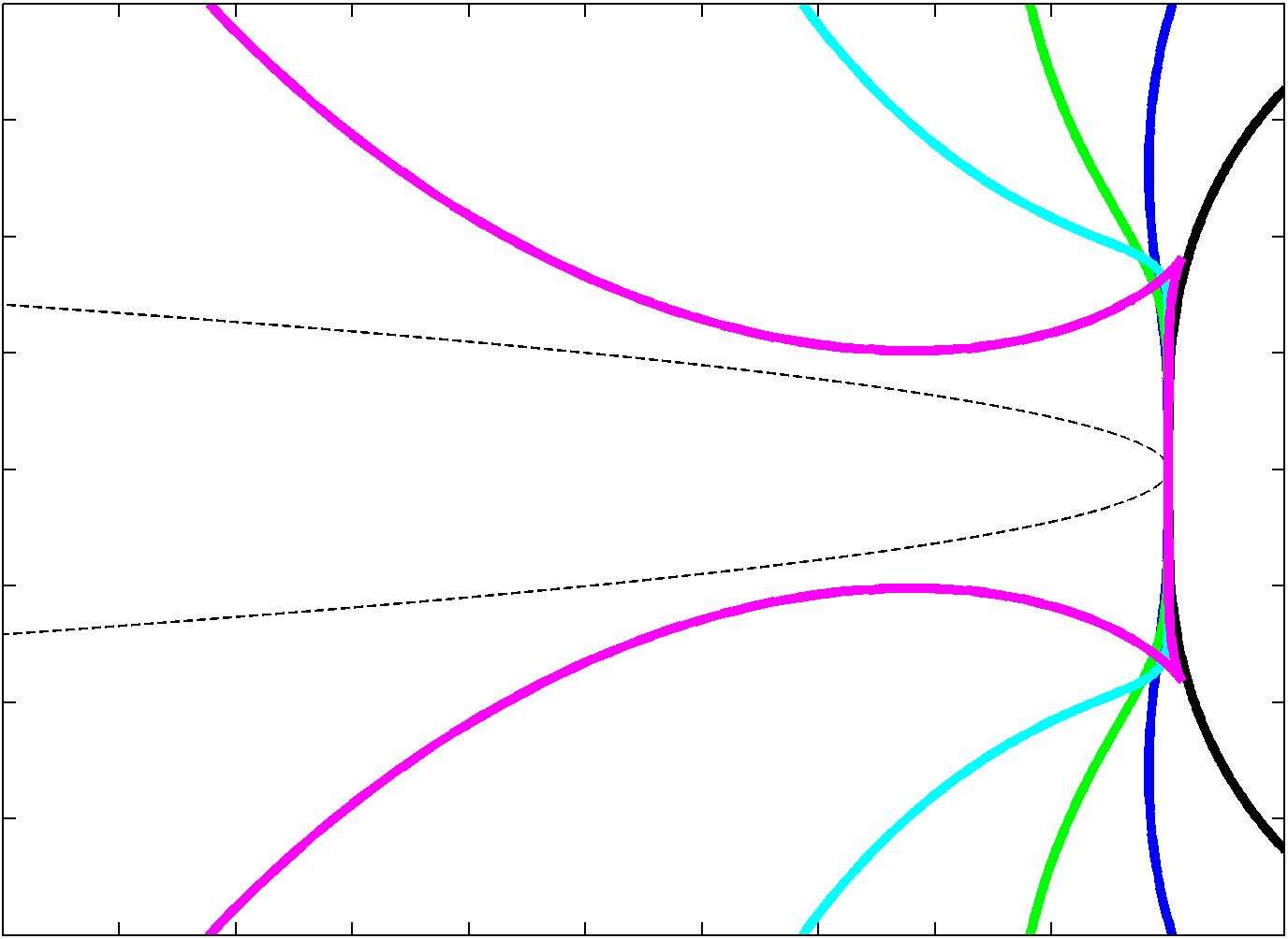
Figure 2: Boundaries of the stability regions of the BDF methods of order $s=2$ (black), 3 (blue), 4 (green), 5 (cyan) and 6 (magenta), together with a parabola $\Gamma_{m}$ (dashed black), $m=0.1$, that is contained in every stability region.

Lemma 3.

Let $\Gamma_{m}$ denote the locus of the left-facing parabola of equation $x=-\frac{1}{m}y^{2}$ ($m>0$). Then, for each $2\leq s\leq 6$, there exists a critical $m$-value $m_{C}$ such that $\Gamma_{m}$ lies in the stability region $R_{s}$ of the BDF method of order $s$ for all $0\leq m<m_{C}$.

Proof.

Clearly, given $s=1,\dots,6$, $\Gamma_{m}$ is contained within $R_{s}$ (see Figure 2) if and only if $m$ is larger than the infimum

$$m_{C}=\inf\left\{m\,|\,m=-\frac{y^{2}}{x}\,\mbox{for some}\,(x+iy)\in R_{s}\right\}.$$ (92)

Simple geometrical considerations, further, show that $m_{C}$ is a positive number (details in these regards can be found in [5, Sec. 2.4]; consideration of Figure 2, however, clearly indicates that $m_{C}>0$). Thus, the parabola $\Gamma_{m}$ is contained within $R_{s}$ if and only if $0\leq m<m_{C}$, and the proof is complete. ∎

Numerical values of $m_{C}$ for each BDF method of orders 3 through 6 (which were computed as the infimum of $-\frac{y^{2}}{x}$ over the boundary of $R_{s}$), are presented in Table 1.

$s$	3	4	5	6
$m_{C}$	14.0	5.12	1.93	0.191

Table 1: Numerical values of the constant $m_{C}$ obtained via numerical evaluation of equation (92). For all $m<m_{C}$ the parabola $\Gamma_{m}$ described in Lemma 3 is contained in the region of absolute stability of the BDF method of order $s$. By Theorem 4, the order-$s$ BDF method applied to the advection-diffusion equation $u_{t}+\alpha\,u_{x}=\beta\,u_{xx}$ with Fourier collocation is stable for all $\Delta t<\frac{\beta}{\alpha^{2}}m_{C}$.

Theorem 4.

Let $2\leq s\leq 6$. The solution produced for the problem (89) by the $s$-th order Fourier-based BDF scheme described in this section is quasi-unconditionally stable (Definition 1) with $M_{h}=\infty$ and $M_{t}=\frac{\beta}{\alpha^{2}}m_{C}$ ($M_{t}=\infty$ for $\alpha=0$), where the $s$ dependent constant $m_{C}$ is given in equation (92).

Proof.

Applying the discrete Fourier transform,

$$\widehat{u}_{k}=\frac{1}{N+1}\sum_{j=0}^{N}u_{j}e^{-ix_{j}k},\quad-\frac{N}{2}\leq k\leq\frac{N}{2}$$

to equation (90) we obtain the set of ODEs

$$\frac{\partial}{\partial t}\widehat{u}_{k}=-(i\alpha k+\beta k^{2})\,\widehat{u}_{k}$$ (93)

for the Fourier coefficients $\widehat{u}_{k}$. It is clear from this transformed equation that the eigenvalues of the spatial operator for the semi-discrete system are given by

$$\lambda(k)=-(i\alpha k+\beta k^{2}).$$ (94)

In view of Remark 2, to complete the proof it suffices to show that these eigenvalues multiplied by $\Delta t$ lie in the stability region of the BDF method for all $\Delta t<\frac{\beta}{\alpha^{2}}m_{C}$.

Let $z_{k}=\lambda(k)\,\Delta t$. If $\alpha=0$, then $z_{k}$ is a non-positive real number for all integers $k$. In view of the A(0)-stability of the BDF methods, we immediately see that the methods are unconditionally stable in this case. For the case $\alpha\neq 0$, in turn, we have

$$z_{k} =\lambda(k)\Delta t=-\beta\,\Delta t\,k^{2}-i\alpha\,\Delta t\,k$$

$$=-\frac{\beta}{\alpha^{2}\Delta t}(\alpha\,\Delta t\,k)^{2}-i(\alpha\,\Delta t\,k)$$

$$=-\frac{1}{\frac{\alpha^{2}\Delta t}{\beta}}(\alpha\,\Delta t\,k)^{2}-i(\alpha\,\Delta t\,k)\quad\mbox{with}\quad-\frac{N}{2}\leq k\leq\frac{N}{2}.$$ (95)

From (95) it is clear that, for all integers $k$, $z_{k}$ lies on the left-facing parabola $\Gamma_{m}$ with

$$m=\frac{\alpha^{2}\Delta t}{\beta}.$$ (96)

But, by Lemma 3 we know that the parabola $\Gamma_{m}$ lies within the stability region $R_{s}$ for all $m<m_{C}$, and, thus, for all

$$\Delta t<\frac{\beta}{\alpha^{2}}m_{C}.$$

Furthermore, the above condition holds for all $N$ and all $k$ with $-N/2\leq k\leq N/2$. It follows that $M_{h}=\infty$ and the proof is complete. ∎

We now establish the quasi-unconditional stability of the Fourier-based BDF methods for the advection-diffusion equation

$$u_{t}+\boldsymbol{\alpha}\cdot\nabla u=\beta\Delta u,\quad\text{ in }[0,2\pi]^{d},\ d=2,3$$ (97)

in two- and three-dimensional space and with periodic boundary conditions, where $\boldsymbol{\alpha}=(\alpha_{1},\alpha_{2})^{\mathrm{T}}$ and $\boldsymbol{\alpha}=(\alpha_{1},\alpha_{2},\alpha_{3})^{\mathrm{T}}$ for $d=2$ and 3 respectively. Thus, letting $\mathbf{x}=(x,y)^{\mathrm{T}}$, $\mathbf{k}=(k_{x},k_{y})^{\mathrm{T}}$, $\mathbf{N}=(N_{x},N_{y})^{\mathrm{T}}$ (resp. $\mathbf{x}=(x,y,z)^{\mathrm{T}}$, $\mathbf{k}=(k_{x},k_{y},k_{z})^{\mathrm{T}}$, $\mathbf{N}=(N_{x},N_{y},N_{z})^{\mathrm{T}}$) in $d=2$ (resp. $d=3$) spatial dimensions, and substituting the Fourier series (using multi-index notation)

$$u(\mathbf{x})=\sum_{\mathbf{k}=-\mathbf{N}/2}^{\mathbf{N}/2}\widehat{u}_{\mathbf{k}}e^{i(\mathbf{k}\cdot\mathbf{x})}$$

into equation (97), the Fourier-based BDF method of order $s$ results as the $s$-order BDF method applied to the ODE system

$$\frac{\partial\widehat{u}_{\mathbf{k}}}{\partial t}=\left(-i(\boldsymbol{\alpha}\cdot\mathbf{k})-\beta|\mathbf{k}|^{2}\right)\widehat{u}_{\mathbf{k}}.$$ (98)

for the Fourier coefficients $\widehat{u}_{\mathbf{k}}$. (In order to utilize a single mesh-size parameter $h$ and corresponding quasi-unconditional stability constant $M_{h}$ while allowing for different grid-fineness in the $x$, $y$ and $z$ directions, we utilize positive integers $r_{2}$ and $r_{3}$ and discretize the domain on the basis of $N_{x}+1$ points in the $x$ direction, $N_{y}+1=r_{2}N_{x}+1$ points in the $y$ direction, and $N_{z}+1=r_{3}N_{x}+1$ points in the $z$ direction ($N_{x}$ even). The mesh size parameter is then given by $h=2\pi/(N_{x}+1)$.)

Theorem 5.

The Fourier-based BDF scheme of order $s$ (not ADI!) for the problem (97) with $3\leq s\leq 6$ is quasi-unconditionally stable with constants $M_{t}=\frac{|\boldsymbol{\alpha}|^{2}}{\beta}m_{C}$ and $M_{h}=\infty$.

Proof.

We first note that the eigenvalues of the discrete spatial operator in equation (98) multiplied by $\Delta t$ are given by

$$z_{\mathbf{k}}=-i\Delta t\,\boldsymbol{\alpha}\cdot\mathbf{k}-\Delta t\,\beta|\mathbf{k}|^{2}.$$ (99)

Clearly, in contrast with the situation encountered in the context of the one dimensional problem considered in Theorem 4, in the present case the set of $z_{\mathbf{k}}$ does not lie on a single parabola. But, to establish quasi-unconditional stability it suffices to verify that this set is bounded on the right by a certain left-facing parabola through the origin. This can be accomplished easily: in view of the Cauchy-Schwarz inequality, we have

$$|\boldsymbol{\alpha}\cdot\mathbf{k}|\leq|\boldsymbol{\alpha}||\mathbf{k}|.$$ (100)

Therefore, letting $\xi=|\mathbf{k}|$, the eigenvalues multiplied by $\Delta t$ are confined to the region

$$\{z\,:\,\Re z=-\Delta t\beta\xi^{2},\;|\Im z|\leq\Delta t|\boldsymbol{\alpha}|\xi,\;\xi\geq 0\}.$$

Clearly, the boundary of this region is the left-facing parabola

$$x=-\frac{\beta}{\Delta t|\boldsymbol{\alpha}|^{2}}y^{2}$$

and the theorem now follows from an application of Lemma 3 together with a simple argument similar to the one used in Theorem 4. ∎

5.2 Order-$s$ BDF methods outside the rectangular window of stability

$\begin{array}[]{ccc}\includegraphics[width=117.43874pt]{AdvDiffBDF5_Alt1}&\includegraphics[width=117.43874pt]{AdvDiffBDF5_Alt2}&\includegraphics[width=117.43874pt]{AdvDiffBDF5_Alt3}\\ \text{(a)}&\text{(b)}&\text{(c)}\end{array}$

Figure 3: Variation of the eigenvalue distribution for the one-dimensional advection-diffusion equation with $\alpha=1.0$ and $\beta=0.05$ (parameters selected for clarity of visualization), as $N$ and $\Delta t$ are varied. (Theoretical value: $M_{t}=0.0965$ for this selection of physical parameters.) The eigenvalues associated with this problem multiplied by $\Delta t$ are plotted as red dots together with the corresponding parabola $\Gamma_{m}$ with $m=\alpha^{2}\Delta t/\beta$ (dashed black line) and the boundary of the BDF5 stability region (cyan curve; cf. Figure 2) for various values of $N$ and $\Delta t$. Figure 3(a): $N+1=19$ and $\Delta t=0.15$; in this case some eigenvalues lie outside the stability region. Figure 3(b): The time-step is reduced to $\Delta t=M_{t}=0.0965$, the parabola $\Gamma_{m}$ is tangent to the stability boundary and fully contained in stability region; in particular, all eigenvalues now lie within in the stability region. Figure 3(c) The number of grid points is increased to $N+1=41$ while maintaining stability: for this value of $\Delta t$ stability holds for all values of $N$.

Theorems 4 and 5 should not be viewed as a suggestion that the $s$-th order BDF methods are not stable when the constraint $\Delta t<M_{t}$ in the theorem is not satisfied. For example, for $\Delta t>M_{t}$ the complete parabolas $\Gamma_{m}$ defined in Section 5.1 intersect the region where the BDF method is unstable—as demonstrated in Figure 3. Fortunately, however, stability can still be ensured for such values of $\Delta t$ provided sufficiently large values of the spatial meshsizes are used. For example, in the one-dimensional case considered in Theorem 4 we have $N+1=2\pi/h$, and the eigenvalues are given by equation (95): clearly only a bounded segment in the parabola is actually relevant to the stability of the ODE system that results for each fixed value of $N$. In particular, we see that stability is ensured provided this particular segment, and not necessarily the complete parabola $\Gamma_{m}$, is contained in the stability region of the $s$-th order BDF algorithm.

From equation (95) we see that increases in the values of $N$ lead to corresponding increases in the length of the parabolic segment on which the eigenvalues actually lie, while decreasing $\Delta t$ results in reductions of both the length of the relevant parabolic segment as well as the width of the parabola itself. Therefore, for $\Delta t>M_{t}$, increasing the number of grid points eventually causes some eigenvalues to enter the region of instability. But stability can be restored by a corresponding reduction in $\Delta t$—see Figure 3. In other words, a CFL-like condition of the form $\Delta t\leq F(h)$ ($h=2\pi/(N+1)$) exists for $\Delta t>M_{t}$: the “maximum stable $\Delta t$” function $F(h)$ can be obtained by considering the intersection of the boundary locus of the BDF stability region (equation (91)) and the parabola $\Gamma_{m}$ with $m$ given by equation (96). It can be seen from the first line in equation (95) that, provided the coefficient of $\Delta t$ in the real part is much smaller than the corresponding coefficient of $\Delta t$ in the imaginary part then the CFL-like condition will be approximately linear around that point—as is apparent by consideration of the actual curves $\Delta t_{\mathrm{max}}=F(h)$ in Figure 4 near $h=1$. Of course, when $\Delta t$ is reduced to the value $M_{t}$ or below, then no increases in $N$ (reductions in $h$) result in instability—as may be appreciated by consideration of Figures 3. We may thus emphasize: within the rectangular stability window no such CFL-like stability constraints exist.

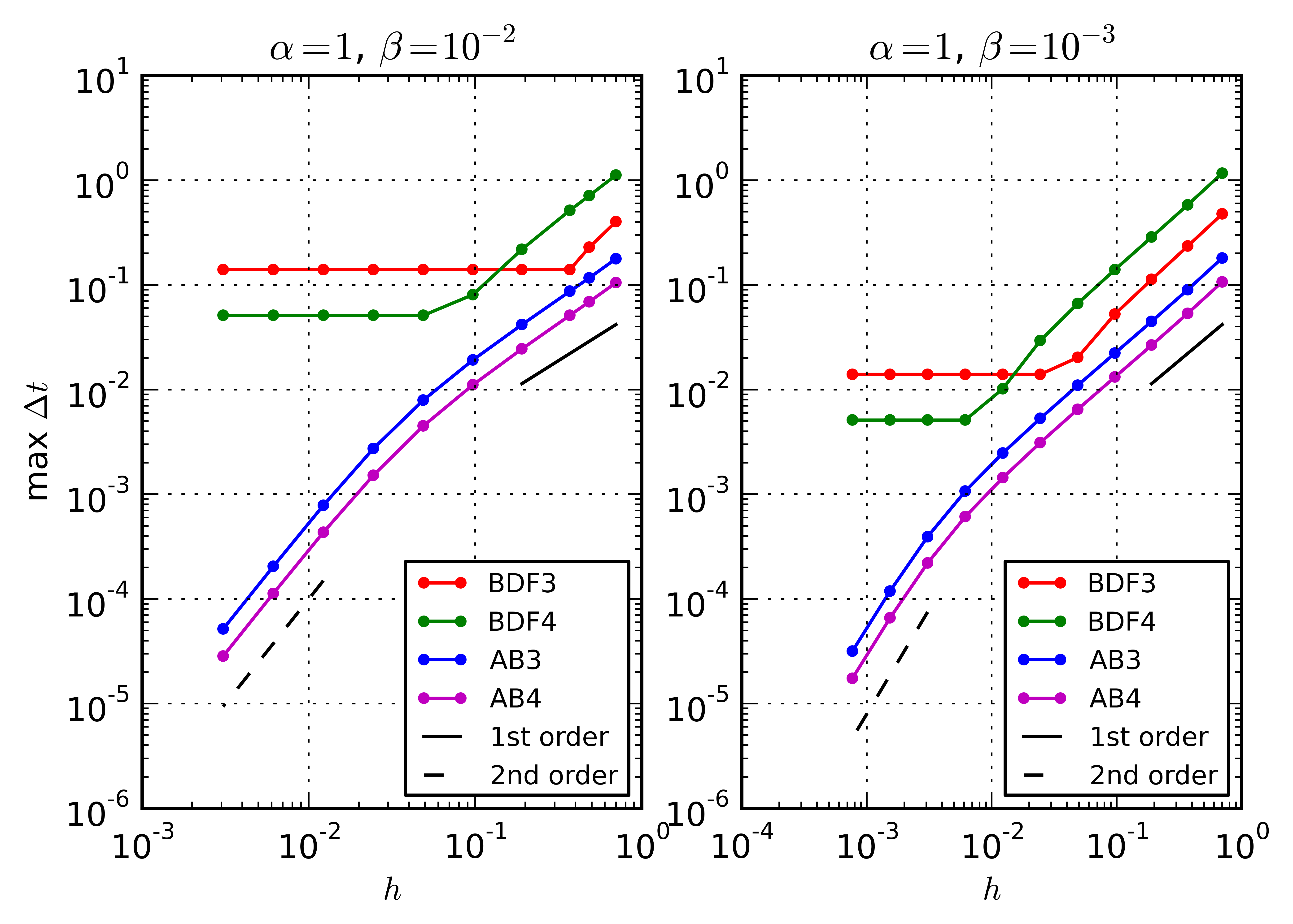
Figure 4: Maximum stable $\Delta t$ versus spatial mesh size $h$ for Fourier-based BDF and AB methods of orders three and four for the advection-diffusion equation (89), with $\alpha=1$, $\beta=10^{-2}$ (left plot) and $\alpha=1$, $\beta=10^{-3}$ (right plot). Both the BDF and AB maximum-stable-$\Delta t$ values were obtained by considering the intersection of the boundary locus of the relevant stability region (either BDF or AB), as indicated in Section 5.2 in the context of the BDF method.

For comparison, Figure 4 also displays the maximum stable $\Delta t$ curves for the Fourier-based Adams-Bashforth (AB) multistep methods of orders three and four as functions of the meshsize $h$ for the advection-diffusion equation under consideration with $\alpha=1$ and two values of $\beta$. We see that the stability of both the BDF and AB methods is controlled by an approximately linear CFL-type constraint of the form $\Delta t<Ch$ for sufficiently large values of $h$. For smaller values of $h$ the CFL condition for the explicit method becomes more severe, and eventually reaches the approximately quadratic regime $\Delta t<Ch^{2}$. By this point, the BDF methods have already entered the window of quasi-unconditional stability. For the particular value of $\alpha$ considered in these examples, at $h=\beta$ the maximum stable $\Delta t$ values for the BDF methods are approximately one hundred times larger than their AB counterparts. Clearly, the BDF methods are preferable in regimes where the AB methods suffer from the severe $\Delta t<Ch^{2}$ CFL condition.

6 Quasi-unconditional stability for the full Navier-Stokes equations: a numerical study

Tables 2, 3 and 4 display numerically estimated maximum stable $\Delta t$ values for the Chebyshev-based BDF-ADI algorithm introduced in Part I for the full Navier-Stokes equations in two dimensional space for various numbers of Chebyshev discretization points. The specific problem under consideration is posed in the unit square $[0,1]\times[0,1]$ with Mach number 0.9 and various Reynolds numbers, with initial condition given by $\mathbf{u}=0$, $\rho=T=1$, and with a source term of the form

$$f(x,y,t)=A\,\sin(2\pi t)\,\exp\left(\,-\frac{1}{2\sigma^{2}}\left(\,(x-x_{0})^{2}+(y-y_{0})^{2}\,\right)\,\right)$$

as the right-hand side of the $x$-coordinate of the momentum equation ($A=6.0$, $\sigma^{2}=0.05$ and $x_{0}=y_{0}=0.5$). No-slip isothermal boundary conditions ($\mathbf{u}=0$, $T=1$) are assumed at $y=0$ and $y=1$, and a sponge layer (see Part I) of thickness $0.1$ and amplitude $2.0$ is enforced at $x=0$ and $x=1$. The algorithm was determined to be stable for a given $\Delta t$ if the solution does not blow up for 20000 time steps or for the number of time steps required to exceed $t=100$, whichever is greater.

Tables 2, 3 and 4 suggest that the BDF-ADI Navier-Stokes algorithm introduced in Part I is indeed quasi-unconditionally stable. In particular, consideration of the tabulated values indicates that the BDF-ADI methods may be particularly advantageous whenever the time-steps required for stability in a competing explicit scheme for a given spatial discretization is much smaller than the time-step required for adequate resolution of the time variation of the solution.

	$s=\dots$
$N_{y}$	2	3	4	5	6
12	6.1e-1	3.5e-1	9.1e-2	4.1e-2	1.7e-2
16	6.1e-1	2.9e-1	8.7e-2	3.2e-2	9.0e-3
24	6.1e-1	1.3e-1	5.9e-2	1.9e-2	5.3e-3
32	6.1e-1	1.2e-1	5.0e-2	1.5e-2	4.3e-3
48	6.1e-1	1.0e-1	4.2e-2	1.3e-2	3.7e-3
64	6.1e-1	1.0e-1	4.1e-2	1.2e-2	3.5e-3
96	6.1e-1	1.0e-1	4.0e-2	1.2e-2	3.1e-3
128	6.1e-1	1.0e-1	4.0e-2	1.2e-2	2.8e-3

Table 2: Maximum stable $\Delta t$ values for the order-$s$ BDF-ADI Navier-Stokes solvers introduced in Part I with $s=2,\dots,6$, in two spatial dimensions, and at Reynolds number $\mathrm{Re}=50$ and Mach number $0.8$, with various numbers $N_{y}$ of discretization points in the $y$ variable. The number of discretization points in the $x$ direction is fixed at $N_{x}=12$.

	$s=\dots$
$N_{y}$	2	3	4	5	6
12	6.4e-1	3.4e-1	5.9e-2	3.4e-2	1.5e-2
16	6.3e-1	2.7e-1	5.0e-2	2.4e-2	9.9e-3
24	6.3e-1	1.1e-1	4.5e-2	1.9e-2	6.1e-3
32	6.3e-1	9.2e-2	3.7e-2	1.7e-2	5.1e-3
48	6.3e-1	7.8e-2	3.2e-2	1.6e-2	4.6e-3
64	6.3e-1	7.4e-2	3.1e-2	1.5e-2	4.4e-3
96	6.3e-1	7.2e-2	3.0e-2	1.5e-2	4.3e-3
128	6.3e-1	7.1e-2	3.0e-2	1.5e-2	4.1e-3

Table 3: Same as Table 3 but with Reynolds number $\mathrm{Re}=100$.

	$s=\dots$
$N_{y}$	2	3	4	5	6
12	5.5e-1	2.9e-1	4.5e-2	2.8e-2	1.3e-2
16	5.3e-1	2.9e-1	4.4e-2	2.0e-2	8.8e-3
24	5.5e-1	1.1e-1	2.5e-2	1.3e-2	4.6e-3
32	5.4e-1	8.6e-2	2.3e-2	1.1e-2	3.6e-3
48	5.3e-1	6.6e-2	2.1e-2	9.5e-3	2.9e-3
64	5.3e-1	6.1e-2	2.1e-2	8.2e-3	2.9e-3
96	5.3e-1	5.9e-2	2.1e-2	8.3e-3	2.4e-3
128	5.3e-1	5.8e-2	2.1e-2	8.2e-3	2.5e-3

Table 4: Same as Table 2 but with Reynolds number $\mathrm{Re}=200$.

7 Summary and conclusions

A variety of studies were put forth in this paper concerning the stability properties of the compressible Navier-Stokes BDF-ADI algorithms introduced in Part I, including rigorous stability proofs for associated BDF- and BDF-ADI-based algorithms for related linear equations, and numerical stability studies for the fully nonlinear problem. In particular, the present paper presents proofs of unconditional stability or quasi-unconditional stability for BDF-ADI schemes as well as certain associated un-split BDF schemes, for a variety of diffusion and advection-diffusion linear equations in one, two and three dimensions, and for schemes of orders $2\leq s\leq 6$ of temporal accuracy. (The very concept of quasi-unconditional stability was introduced in Part I to describe the observed stability character of the Navier-Stokes BDF-ADI algorithms introduced in that paper.) A set of numerical experiments presented in this paper for the compressible Navier-Stokes equation suggests that the algorithms introduced in Part I do enjoy the claimed property of quasi-unconditional stability.

Acknowledgments

The authors gratefully acknowledge support from the Air Force Office of Scientific Research and the National Science Foundation. MC also thanks the National Physical Science Consortium for their support of this effort.

References

- [1] R. M. Beam and R. Warming. An implicit factored scheme for the compressible Navier-Stokes equations. AIAA journal, 16(4):393–402, 1978.
- [2] R. M. Beam and R. Warming. Alternating direction implicit methods for parabolic equations with a mixed derivative. SIAM Journal on Scientific and Statistical Computing, 1(1):131–159, 1980.
- [3] H. Bijl, M. H. Carpenter, V. N. Vatsa, and C. A. Kennedy. Implicit time integration schemes for the unsteady compressible Navier–Stokes equations: laminar flow. Journal of Computational Physics, 179(1):313–329, June 2002.
- [4] O. P. Bruno and M. Cubillos. Higher-order in time “quasi-uncondionally stable” ADI solvers for the compressible Navier-Stokes equations in 2d and 3d curvilinear domains. 2015.
- [5] M. Cubillos. General-domain compressible Navier-Stokes solvers exhibiting quasi-unconditional stability and high-order accuracy in space and time. PhD, California Institute of Technology, Mar. 2015.
- [6] G. G. Dahlquist. A special stability problem for linear multistep methods. BIT Numerical Mathematics, 3(1):27–43, Mar. 1963.
- [7] J. Douglas Jr. and J. E. Gunn. A general formulation of alternating direction methods. Numerische Mathematik, 6(1):428–453, Dec. 1964.
- [8] D. Forti and L. Dedè. Semi–implicit BDF time discretization of the Navier–Stokes equations with VMS–LES modeling in a high performance computing framework. Computers & Fluids, 2015.
- [9] D. Gottlieb and J. S. Hesthaven. Spectral methods for hyperbolic problems. Journal of Computational and Applied Mathematics, 128(1):83–131, 2001.
- [10] B. Gustafsson, H. Kreiss, and J. Oliger. Time-dependent problems and difference methods. Pure and Applied Mathematics: A Wiley Series of Texts, Monographs and Tracts. Wiley, 2013.
- [11] J. S. Hesthaven, S. Gottlieb, and D. Gottlieb. Spectral methods for time-dependent problems, volume 21. Cambridge University Press, 2007.
- [12] S. Karaa. A hybrid Padé ADI scheme of higher-order for convection–diffusion problems. International Journal for Numerical Methods in Fluids, 64(5):532–548, 2010.
- [13] D. A. Kopriva. Implementing spectral methods for partial differential equations: Algorithms for scientists and engineers. Springer Science & Business Media, 2009.
- [14] J. D. Lambert. Numerical methods for ordinary differential systems: the initial value problem. John Wiley & Sons, Inc., 1991.
- [15] R. LeVeque. Finite difference methods for ordinary and partial differential equations. Society for Industrial and Applied Mathematics, Jan. 2007.
- [16] D. W. Peaceman and H. H. Rachford, Jr. The numerical solution of parabolic and elliptic differential equations. Journal of the Society for Industrial and Applied Mathematics, 3(1):28–41, Mar. 1955.
- [17] J. C. Strikwerda. Finite difference schemes and partial differential equations. SIAM, 2004.
- [18] L. N. Trefethen. Pseudospectra of linear operators. SIAM review, 39(3):383–406, 1997.
- [19] L. N. Trefethen and M. Embree. Spectra and pseudospectra: the behavior of nonnormal matrices and operators. Princeton University Press, 2005.
- [20] R. F. Warming and R. M. Beam. An extension of A-stability to alternating direction implicit methods. BIT Numerical Mathematics, 19(3):395–417, Sept. 1979.