A Second Order Time Homogenized Model for Sediment Transport

Abstract.

A multi-scale method for the hyperbolic systems governing sediment transport in subcritical case is developed. The scale separation of this problem is due to the fact that the sediment transport is much slower than flow velocity. We first derive a zeroth order homogenized model, and then propose a first order correction. It is revealed that the first order correction for hyperbolic systems has to be applied on the characteristic speed of slow variables in one dimensional case. In two dimensional case, besides the characteristic speed, the source term is also corrected. We develop a second order numerical scheme following the framework of heterogeneous multi-scale method. The numerical results in both one and two dimensional cases demonstrate the effectiveness and efficiency of our method.

Keywords. homogenization, multi-scale method, first order correction, sediment transport

AMS subject classifications. 65M08, 76M45, 76M50

The sediment transport in flow is often modelled by a scalar convective equation coupled with the shallow water equations. Typically, the morphodynamic process by sediment transport is an extremely slow process [1, 2] in term of the flow velocity in the model, while the changes in the topography are usually of practical interests. Since interesting changes in the topography can only be produced by the continual erosion of the flow for a long period of time, the model is provided a scale separation in time. In the coupled model of the sediment transport equation and the shallow water equations, the system of shallow water equations is of standard formation, with the contribution from the riverbed elevation. In the past decades, the spatial variation of the riverbed elevation has been extensively investigated [3]. The expressions of the sediment tranport flow are usually proposed for granular non-cohesive sediments and quantified empirically [4, 5, 6, 7, 8, 9, 10].

In this paper, we consider the following widely used system to model the sediment transport in one dimensional case

(0.1) $$\left\{\begin{aligned} &\partial_{t}h+\partial_{x}(hu)=0,\\ &\partial_{t}(hu)+\partial_{x}(hu^{2}+\frac{1}{2}gh^{2})=-gh\partial_{x}B,\\ &\partial_{t}B+\xi\partial_{x}q_{b}=0,\end{aligned}\right.$$

where the first two equations are the shallow water equations, and the last equation is the Exner equation [11, 12] involving a sediment transport flux. In this system, $h$ is the water depth, $u$ is the vertically averaged flow velocity along the $x$ direction, and $B$ is the riverbed elevation. $q_{b}$ denotes the volumetric bedload sediment transport discharge. Different from the standard shallow water equations, the riverbed elevation $B$ depends on time $t$ as well. The parameters involved are the gravity constant $g$ and $\xi=(1-\gamma)^{-1}$ with $\gamma$ the porosity of sediment layer. Grass [4] proposed one of the simplest formulation of $q_{b}$ as

(0.2) $$q_{b}=A_{g}u|u|^{m-1}\qquad 1\leq m\leq 4,A_{g}\in(0,1].$$

In practice, estimates of the bedload transport rate are mainly based on the modeling of bottom shear stress $\tau_{b}$ and a non-dimensional parameters $q_{b}^{*}$ as

$$q_{b}=q_{b}^{*}\sqrt{(s-1)gd_{s}^{3}},$$

where $s$ is the density ratio between sediment $\rho_{s}$ and water $\rho$, and $d_{s}$ is the median diameter of sediment. The non-dimensional form of bottom shear stress, which is also called Shields parameter, is defined as

$$\tau_{b}^{*}=\frac{\tau_{b}}{(s-1)\rho gd_{s}}.$$

A variety of models [4, 5, 6, 7, 8, 9, 10] have been often applied to build the relationship between $q_{b}^{*}$ and Shields parameter. In this paper, one of the most commonly-used models proposed by Meyer, Peter and Müler [5] is considered:

(0.3) $$q_{b}^{*}=8(\tau_{b}^{*}-\tau_{cr}^{*})_{+}^{3/2}:=\begin{cases}8(\tau_{b}^{*}-\tau_{cr}^{*})^{3/2}&\text{if}~{}\tau_{b}^{*}>\tau_{cr},\\ 0&\text{otherwise}.\end{cases}$$

Consider the Darcy-Weisbach formula for the bottom shear stress in the context of laminar flows, we have

$$\tau_{b}=\rho ghS_{f}\qquad S_{f}=\frac{fu|u|}{8gh},$$

where $f$ is the Darcy-Weisbach’s coefficient. Consequently, the original Meyer-Peter-Müler model (0.3) can be reduced to the following expression,

(0.4) $$q_{b}=8\sqrt{(s-1)gd_{s}^{3}}\frac{u}{|u|}\left(\frac{f}{8(s-1)gd_{s}}|u|^{2}-\tau_{cr}^{*}\right)^{3/2}.$$

The Grass model (0.2) and Meyer-Peter-Müler model (0.4) can be recast into a unified fashion as

(0.5) $$\xi q_{b}=\varepsilon u\tilde{q}_{b}(|u|),$$

where

• For Grass model (0.2):

  (0.6) $$\varepsilon=\xi A_{g}\qquad\text{and}\qquad\tilde{q}_{b}(|u|)=|u|^{m-1}\qquad 1\leq m\leq 4.$$

• For Meyer-Peter-Müler model (0.4):

  (0.7) $$\varepsilon=\frac{\xi}{(s-1)g}\sqrt{\frac{f^{3}}{8}}\qquad\text{and}\qquad\tilde{q}_{b}(|u|)=\frac{1}{|u|}(|u|^{2}-u_{cr}^{2})_{+}^{3/2}.$$

  Here the critical velocity $u_{cr}=\sqrt{8(s-1)gd_{s}\tau_{cr}^{*}/f}$. We note that this model is one of the commonly-used for rivers and channels with slope lower than $2\%$, see [13] for details.

For the case that the flow-sediment interaction is low, $\varepsilon$ is far less than the magnitude of typical flow velocity to depict the scale separation in time. In this sense, we call the parameter $\varepsilon$ in (0.5) the time scaling parameter.

Similarly, the governing system in two dimensional case is formulated as

(0.8) $$\dfrac{\partial}{\partial t}\begin{pmatrix}h\\ hu\\ hv\\ B\end{pmatrix}+\dfrac{\partial}{\partial x}\begin{pmatrix}hu\\ hu^{2}+\frac{1}{2}gh^{2}\\ huv\\ \varepsilon u\tilde{q}_{b}(|\mathbf{u}|)\end{pmatrix}+\dfrac{\partial}{\partial y}\begin{pmatrix}hv\\ huv\\ hv^{2}+\frac{1}{2}gh^{2}\\ \varepsilon v\tilde{q}_{b}(|\mathbf{u}|)\end{pmatrix}=\begin{pmatrix}0\\ -ghB_{x}\\ -ghB_{y}\\ 0\end{pmatrix},$$

where $\mathbf{u}=(u,v)^{T}$ is the vertically averaged flow velocity along the $x$ and $y$ direction.

The scale separation in time brings us serious difficulty in carrying out numerical simulation for (0.1) or (0.8). Currently, there are two classifications of the numerical methods for this problem: coupled method and decoupled method. The decoupled method is suitable for the case that the topography changes much slower than the flow, which results in a quasi-steady water motions with respect to the topography. It was pioneered by Cunge et al. [2], and has been widely used in industry [3, 14, 15] on account of its high computational efficiency. There are, however, two drawbacks associated with decoupled method, including the instability when updating the riverbed with traditional scheme (e.g. Lax-Wendroff scheme) [16, 17, 18] and the low accuracy in terms of $\varepsilon$.

With the purpose of overcoming the above drawbacks of the decoupled method, much effort has been devoted to develop numerical schemes by coupling the hydrodynamics and morphodynamics. The numerical techniques developed in this fold include the Roe-type scheme [16, 19, 20, 21, 22, 23, 24], the second order LHLL method [25], the balanced finite volume WENO scheme [26], the state reconstructions for non-conservation hyperbolic systems [27], the relaxation approximation [28], the second order SRNHS scheme [29], the WAF method [30], the McCormack scheme [31], etc. One of the main difficulties for coupled method comes from the fact that the interaction between fluid and sediment is usually too weak [27], and the simulations have to carry out for a long time. Therefore, it is necessary to use high order numerical schemes to depress the numerical dissipation. At the same time, one has to suffer by the small time step size restricted by the hydrodynamic time scale for the explicit scheme. Recently, the linearized implicit method [32] was proposed to enlarge the time step size.

The multi-scale method we developed in this paper for the sediment transport problem looks somewhat like the decoupled method. In the subcritical case, we first reformulate the sediment transport model to a non-conservative scalar equation (or the zeroth order equation), which preserves the hyperbolicity of the coupled system. We assume that the morphodynamic process is governed by a limiting equation (or the zeroth order equation) when the time scaling parameter $\varepsilon$ tends to zero. For one dimensional case, the resulting limiting equation is exactly same as the result of De Vries [33]. For two dimensional case, the limiting equation can be derived subsequently as a reasonable extension of the one dimensional case, with a difference in the source term. When developing the numerical method in the framework of Heterogeneous Multiscale Method (HMM) [34], the steady state solver for shallow water equations is adopted as the micro-solver, and the macro-solver for the morphodynamic time scale dynamics is applied. Therefore, the first drawback of decoupled method can be avoided to some extent by taking a stable scheme for zeroth order model as the macro-solver when updating the riverbed topography.

For practical problems that the time scaling parameter $\varepsilon$ is not so extremely close to zero [27], a first order correction have to be made to improve the order of accuracy for $\varepsilon$. In other words, the model error will be $\mathcal{O}(\varepsilon^{2})$ after the first order correction, which does alleviate the second drawback of decoupled method for the low-interaction between flow and sediment ($\varepsilon\ll 1$).

The basic idea of the first order correction is as follows. With the help of the zeroth order model, two correction terms are applied to the steady state of shallow water equations: the dynamic term used to balance the flux and source term, and the $\mathcal{O}(\varepsilon)$ term. In light of this correction for flow variables, the characteristic speed of riverbed is corrected in one dimensional case, and both the characteristic speed and the source term of riverbed are corrected in two dimensional case. As for the numerical algorithm, an interesting observation is that one can update the flow variables while updating the riverbed topography in the macro time step of morphodynamic time scale. This fast variables correction improves not only the computing accuracy but also the stability of the numerical multi-scale method.

The rest part of this paper is organized as follows. In section 1, we apply our multi-scale method to one dimensional linear model to describe its key ingredients. In section 2, we give the homogenization of the model in one dimensional case and in section 3, we give the two dimensional model subsequently. In section 4, we develop the corresponding numerical method. The numerical results are in section 5 and a short conclusion remarks in section 6 close the main text.

1. One Dimensional Linear Model

In order to clarify our method for nonlinear hyperbolic systems (0.1) and (0.8), we first present our basic idea by studying the one dimensional linear hyperbolic system as follows

(1.1) $$\left\{\begin{aligned} &\mathbf{U}_{t}+\mathbf{A}\mathbf{U}_{x}=-\mathbf{g}B_{x},\\ &B_{t}+\varepsilon\mathbf{c}^{T}\mathbf{U}_{x}=0.\end{aligned}\right.$$

where $\mathbf{U}=(u_{1},\cdots,u_{l})^{T}\in\mathbb{R}^{l}$ are fast variables, $B\in\mathbb{R}$ is slow variable, $\mathbf{g},\mathbf{c}$ are two constant vectors in $\mathbb{R}^{l}$. The constant matrix $\mathbf{A}\in\mathbb{R}^{l\times l}$ satisfies

(1.2) $$\mathbf{A}=\mathbf{X}^{-1}\mathbf{\Lambda},\mathbf{X}\qquad\mathbf{\Lambda}=\text{diag}\{\lambda_{1},\cdots,\lambda_{l}\}.$$

With the purpose of scale separation on the characteristic speeds of (1.1), it requires $|\lambda_{i}|\gg\varepsilon$, thus $\mathbf{A}$ is invertible. Moreover, we assume $\mathbf{A}$ has only discrete eigenvalues (i.e. the algebraic multiplicity is one). We emphasize that $t$ represents the fast time scale, and $\tau=\varepsilon t$ represents the slow time scale in the context of this paper.

Let

(1.3) $$\mathbf{C}=\begin{pmatrix}\mathbf{A}&\mathbf{g}\\ 0&0\\ \end{pmatrix},\qquad\mathbf{C}^{\varepsilon}=\begin{pmatrix}\mathbf{A}&\mathbf{g}\\ \varepsilon\mathbf{c}^{T}&0\\ \end{pmatrix},\qquad\mathbf{V}=\begin{pmatrix}\mathbf{U}\\ B\end{pmatrix}.$$

Then, the original system (1.1) can be recast as:

$$\mathbf{V}_{t}+\mathbf{C}^{\varepsilon}\mathbf{V}_{x}=0.$$

It follows from (1.2) that $\mathbf{C}=\mathbf{K}^{-1}\mathbf{D}\mathbf{K}$, where

$$\mathbf{K}=\begin{pmatrix}\mathbf{X}&\mathbf{\Lambda}^{-1}\mathbf{X}\mathbf{g}\\ 0&1\end{pmatrix},\qquad\mathbf{D}=\begin{pmatrix}\mathbf{\Lambda}&0\\ 0&0\end{pmatrix}.$$

By the perturbation theory of discrete eigenvalues and eigenvectors in [35],

(1.4) $$\mathbf{C}^{\varepsilon}=(\mathbf{K}^{\varepsilon})^{-1}\mathbf{D}^{\varepsilon}\mathbf{K}^{\varepsilon},$$

where

$$\mathbf{K}^{\varepsilon}=\begin{pmatrix}\mathbf{X}+\varepsilon\hat{\mathbf{X}}&\mathbf{\Lambda}^{-1}\mathbf{X}\mathbf{g}+\varepsilon\hat{\mbox{\boldmath$\alpha$}}\\ \varepsilon\hat{\mbox{\boldmath$\beta$}}^{T}&1+\varepsilon\hat{\theta}\\ \end{pmatrix},\qquad\mathbf{D}^{\varepsilon}=\begin{pmatrix}\mathbf{\Lambda}+\varepsilon\hat{\mathbf{\Lambda}}&0\\ 0&\varepsilon\mu\\ \end{pmatrix}.$$

1.1. Zeroth order model

The first step of our method is to predict the slow variable $B$. Eliminating the spatial derivative terms of fast variables in (1.1), we have

$$B_{t}+\varepsilon\mathbf{c}^{T}\mathbf{A}^{-1}(-\mathbf{g}B_{x}-\mathbf{U}_{t})=0,$$

that is

(1.5) $$B_{\tau}-\mathbf{c}^{T}\mathbf{A}^{-1}\mathbf{g}B_{x}-\varepsilon\mathbf{c}^{T}\mathbf{A}^{-1}\mathbf{U}_{\tau}=0,$$

The zeroth order model (or limiting equation) for the linear hyperbolic system (1.1) is derived by $\varepsilon\to 0$, namely

(1.6) $$B^{(0)}_{\tau}+\lambda_{B}^{(0)}B^{(0)}_{x}=0,$$

where $\lambda_{B}^{(0)}=-\mathbf{c}^{T}\mathbf{A}^{-1}\mathbf{g}$. We note that the zeroth order model (1.6) is established only on the hypothesis that $\mathbf{U}_{\tau}$ is bounded. In particular, this hypothesis holds when the fast dynamics has a steady state (up to $\mathcal{O}(\varepsilon)$) with fixed slow variable in the initial state. At this point, the zeroth order model (1.6) provides a prediction for $B$ on the interval $[0,\Delta\tau]$ as

$$B^{(0)}(x,\tau)=B(x-\lambda_{B}^{(0)}\tau,0),\qquad\tau\in[0,\Delta\tau].$$

In light of the prediction, a modified fast dynamics $\mathbf{U}^{(1)}$ can be derived which is slightly different from that with fixed slow variable. Our next step is to calculate the difference between the steady variable $\mathbf{U}^{(0)}(x,\tau)$ and $\mathbf{U}^{(1)}(x,\tau)$ to get the correction terms, and by this way the correction model for the riverbed can be obtained. More precisely, we will show this process step by step strictly for the linear system. First, we have the following lemma for zeroth order model (1.6):

Lemma 1.1.

Suppose that $\mathbf{A}\in\mathbb{R}^{l\times l}$ has only real and discrete eigenvalues and all eigenvalues satisfy $|\lambda_{i}|>\delta\gg\varepsilon$ for some positive $\delta$. The initial dynamics satisfy

1. $\mathbf{A}\mathbf{U}_{x}(x,0)+\mathbf{g}B_{x}(x,0)=\mathcal{O}(\varepsilon)$.

2. $B^{(0)}(x,0)=B(x,0)\in W^{1,\infty}(\mathbb{R})$.

Then

$$\|B(x,t)-B^{(0)}(x,t)\|_{\infty}=\mathcal{O}(\varepsilon)\qquad\text{for }~{}t\sim\mathcal{O}(\varepsilon^{-1}).$$

Moreover, if $B(x,0)\in W^{2,\infty}(\mathbb{R})$ and $\mathbf{A}\mathbf{U}_{xx}(x,0)+\mathbf{g}B_{xx}(x,0)=\mathcal{O}(\varepsilon)$, then

$$\|B_{x}(x,t)-B^{(0)}_{x}(x,t)\|_{\infty}=\mathcal{O}(\varepsilon)\qquad\text{for }~{}t\sim\mathcal{O}(\varepsilon^{-1}).$$

Proof.

See Appendix A. ∎

1.2. First order model

Now we consider the case in which $\varepsilon$ is small but does not tend to zero. The basic idea here is to improve the accuracy of the weakly coupled term $-\varepsilon\mathbf{c}^{T}\mathbf{A}^{-1}\mathbf{U}_{\tau}$ by zeroth order model (1.6). More specifically, we first substitute $B$ in (1.1) by the solution of the zeroth order model, i.e.

(1.7) $$\mathbf{U}^{(1)}_{t}+\mathbf{A}\mathbf{U}^{(1)}_{x}=-\mathbf{g}B^{(0)}_{x}(x,t).$$

Then, the corrected equation of $B$ can be derived by (1.5) and (1.7) that

(1.8) $$\hat{B}^{(1)}_{\tau}-\mathbf{c}^{T}\mathbf{A}^{-1}\mathbf{g}\hat{B}^{(1)}_{x}-\varepsilon\mathbf{c}^{T}\mathbf{A}^{-1}\mathbf{U}^{(1)}_{\tau}=0.$$

The following lemma indicates that the error between the solution of (1.8) and original equations (1.1) is of $\mathcal{O}(\varepsilon^{2})$ order.

Lemma 1.2.

Under the same assumptions of Lemma 1.1, and assume the initial dynamics satisfy

1. $(\mathbf{A}+\varepsilon\mathbf{X}^{-1}\mathbf{\Lambda}\hat{\mathbf{X}})\mathbf{U}_{x}(x,0)+(\mathbf{g}+\varepsilon\mathbf{X}^{-1}\mathbf{\Lambda}\hat{\alpha})B_{x}(x,0)=\mathcal{O}(\varepsilon^{2})$.

2. $\mathbf{A}\mathbf{U}_{xx}(x,0)+\mathbf{g}B_{xx}(x,0)=\mathcal{O}(\varepsilon)$.

3. $(\mathbf{A}+\varepsilon\mathbf{A})\mathbf{U}_{x}^{(1)}(x,0)+(\mathbf{g}+\varepsilon\mathbf{g}-\varepsilon\mathbf{A}^{-1}\mathbf{g}\mathbf{c}^{T}\mathbf{A}^{-1}\mathbf{g})B_{x}^{(0)}(x,0)=\mathcal{O}(\varepsilon^{2})$.

4. $B^{(0)}(x,0)=\hat{B}^{(1)}(x,0)=B(x,0)\in W^{2,\infty}(\mathbb{R})$.

Then

$$\lVert B(x,t)-\hat{B}^{(1)}(x,t)\rVert_{\infty}=\mathcal{O}(\varepsilon^{2})\qquad\text{for }~{}t\sim\mathcal{O}(\varepsilon^{-1}).$$

Proof.

See Appendix B. ∎

Remark 1.

It is expected that if we apply the above steps repeatedly (i.e. substitute $B^{(0)}$ in (1.7) by the solution of (1.8), and solve (1.8) where $U^{(1)}$ substituted by the solution of the new equation), the results of better accuracy will be achieved. In nonlinear cases, however, it may be of some difficulties to get the correction terms (which will be introduced later) of more than second order accuracy, so we only consider the model up to second order accuracy, i.e. the first order model.

The equation (1.8) does not provide a convenient way to compute $\hat{B}^{(1)}$ due to the appearance of $\mathbf{U}^{(1)}_{\tau}$. Let us keep in mind that our aim is to deduce an equation which only has the riverbed as the variable (just like (1.6)). To this end, one needs to represent $\mathbf{U}^{(1)}_{\tau}$ by the riverbed up to the accuracy of order $\mathcal{O}(\varepsilon^{2})$.

Suppose $\mathbf{U}^{(0)}$ is the steady state when $B$ is fixed to $B^{(0)}(x,0)$, namely $\mathbf{U}^{(0)}_{\tau}=0$. This implies that $(\mathbf{U}^{(1)}-\mathbf{U}^{(0)})_{\tau}=\mathbf{U}^{(1)}_{\tau}$, and thereafter we consider $\mbox{\boldmath$\varphi$}=\mathbf{U}^{(1)}-\mathbf{U}^{(0)}$ other than $\mathbf{U}^{(1)}$. This trick is also used for the nonlinear systems: instead of solving the coupled equations to get $\mathbf{U}^{(1)}_{\tau}$, we use the steady state $\mathbf{U}^{(0)}$ and calculate the difference $\varphi$ to obtain $\mathbf{U}^{(1)}$. Now, we derive the closed form of $\varphi$.

First, we have the following equations:

$$\varepsilon\mathbf{U}^{(0)}_{\tau}+\mathbf{A}\mathbf{U}^{(0)}_{x} =-\mathbf{g}B^{(0)}_{x}(x,0),$$

$$\varepsilon\mathbf{U}^{(1)}_{\tau}+\mathbf{A}\mathbf{U}^{(1)}_{x} =-\mathbf{g}B^{(0)}_{x}(x-\lambda_{B}^{(0)}\tau,0).$$

Taking the difference of the above dynamics and applying the characteristic decomposition of $\mathbf{A}$, we have

(1.9) $$\mathbf{X}\mbox{\boldmath$\varphi$}_{\tau}+\frac{\mathbf{\Lambda}}{\varepsilon}\mathbf{X}\mbox{\boldmath$\varphi$}_{x}=-\frac{\mathbf{X}\mathbf{g}}{\varepsilon}\big{(}B^{(0)}_{x}(x-\lambda^{(0)}_{B}\tau,0)-B^{(0)}_{x}(x,0)\big{)}.$$

The initial condition of $\varphi$ can be derived from Lemma 1.2 and steady state of $\mathbf{U}^{(0)}$, i.e.

(1.10) $$\mathbf{X}\mbox{\boldmath$\varphi$}_{x}(x,0)=\varepsilon\mathbf{\Lambda}^{-2}\mathbf{X}\mathbf{g}\mathbf{c}^{T}\mathbf{A}^{-1}\mathbf{g}B_{x}^{(0)}(x,0)+\mathcal{O}(\varepsilon^{2}).$$

Then, (1.9) can be solved analytically by the method of characteristics as

$$(\mathbf{X}\mbox{\boldmath$\varphi$})_{k}(x,\tau)$$

$$= (\mathbf{X}\mbox{\boldmath$\varphi$})_{k}(x-\frac{\lambda_{k}}{\varepsilon}\tau,0)$$

$$-\frac{(\mathbf{X}\mathbf{g})_{k}}{\varepsilon}\int_{0}^{\tau}B^{(0)}_{x}\big{(}x-\frac{\lambda_{k}}{\varepsilon}\tau+(\frac{\lambda_{k}}{\varepsilon}-\lambda_{B}^{(0)})s,0\big{)}-B^{(0)}_{x}\big{(}x-\frac{\lambda_{k}}{\varepsilon}\tau+\frac{\lambda_{k}}{\varepsilon}s,0\big{)}{\mathrm{d}}s$$

$$= -\frac{(\mathbf{X}\mathbf{g})_{k}}{(\lambda_{k}-\varepsilon\lambda_{B}^{(0)})}B^{(0)}(x-\lambda_{B}^{(0)}\tau,0)+\frac{(\mathbf{X}\mathbf{g})_{k}}{\lambda_{k}}B^{(0)}(x,0)$$

$$+(\mathbf{X}\mbox{\boldmath$\varphi$})_{k}(x-\frac{\lambda_{k}}{\varepsilon}\tau,0)+\frac{\varepsilon(\mathbf{X}\mathbf{g})_{k}\lambda_{B}^{(0)}}{\lambda_{k}(\lambda_{k}-\varepsilon\lambda_{B}^{(0)})}B^{(0)}(x-\frac{\lambda_{k}}{\varepsilon}\tau,0).$$

That is,

$$(\mathbf{X}\mbox{\boldmath$\varphi$})_{k}(x,\tau)= -\frac{\varepsilon(\mathbf{X}\mathbf{g})_{k}\lambda_{B}^{(0)}}{\lambda_{k}(\lambda_{k}-\varepsilon\lambda_{B}^{(0)})}B^{(0)}(x,0) \cdots\cdots~{}\mathcal{O}(\varepsilon)~{}\text{term}$$

(1.11) $$-\frac{(\mathbf{X}\mathbf{g})_{k}}{(\lambda_{k}-\varepsilon\lambda_{B}^{(0)})}\big{(}B^{(0)}(x-\lambda_{B}^{(0)}\tau,0)-B^{(0)}(x,0)\big{)} \cdots\cdots~{}\mathcal{O}(\tau)~{}\text{term}$$

$$+(\mathbf{X}\mbox{\boldmath$\varphi$})_{k}(x-\frac{\lambda_{k}}{\varepsilon}\tau,0) \cdots\cdots~{}\text{high order term}$$

$$+\frac{\varepsilon(\mathbf{X}\mathbf{g})_{k}\lambda_{B}^{(0)}}{\lambda_{k}(\lambda_{k}-\varepsilon\lambda_{B}^{(0)})}B^{(0)}(x-\frac{\lambda_{k}}{\varepsilon}\tau,0). \cdots\cdots~{}\text{high order term}$$

We will show later that the last two terms provide $\mathcal{O}(\varepsilon^{2})$ term in the error estimation. This is why they are called high order terms. In the nonlinear system, the correction term will be shown to have a similar form.

Denote $\mathbf{e}_{k}(k=1,\cdots,l)$ the unit vectors of $\mathbb{R}^{l}$ and ${\text{diag}}(\mathbf{x})$ the diagonal matrix with vector $\mathbf{x}$ in its diagonal entries. By the decomposition (1.11) and initial condition (1.10), we have

$$\mbox{\boldmath$\varphi$}_{\tau}(x,\tau)= ~{}\lambda_{B}^{(0)}\mathbf{X}^{-1}(\mathbf{\Lambda}-\varepsilon\lambda_{B}^{(0)}\mathbf{I})^{-1}\mathbf{X}\mathbf{g}B_{x}^{(0)}(x-\lambda_{B}^{(0)}\tau,0)$$

$$~{}-\frac{1}{\varepsilon}\mathbf{X}^{-1}\mathbf{\Lambda}\left(\sum_{k=1}^{l}(\mathbf{X}\mbox{\boldmath$\varphi$}_{x})_{k}(x-\frac{\lambda_{k}}{\varepsilon}\tau,0)\mathbf{e}_{k}\right)$$

$$-\lambda_{B}^{(0)}\mathbf{X}^{-1}(\mathbf{\Lambda}-\varepsilon\lambda^{(0)}_{B}\mathbf{I})^{-1}{\text{diag}}(\mathbf{X}\mathbf{g})\left(\sum_{k=1}^{l}B^{(0)}_{x}(x-\frac{\lambda_{k}}{\varepsilon}\tau,0)\mathbf{e}_{k}\right)$$

$$= ~{}\lambda_{B}^{(0)}\mathbf{X}^{-1}\mathbf{\Lambda}^{-1}\mathbf{X}\mathbf{g}B_{x}^{(0)}(x-\lambda_{B}^{(0)}\tau,0)$$

$$~{}-\mathbf{X}^{-1}\mathbf{\Lambda}^{-1}{\text{diag}}(\mathbf{X}\mathbf{g}\mathbf{c}^{T}\mathbf{A}^{-1}\mathbf{g})\left(\sum_{k=1}^{l}B^{(0)}_{x}(x-\frac{\lambda_{k}}{\varepsilon}\tau,0)\mathbf{e}_{k}\right)$$

$$~{}-\lambda_{B}^{(0)}\mathbf{X}^{-1}\mathbf{\Lambda}^{-1}{\text{diag}}(\mathbf{X}\mathbf{g})\left(\sum_{k=1}^{l}B^{(0)}_{x}(x-\frac{\lambda_{k}}{\varepsilon}\tau,0)\mathbf{e}_{k}\right)+\mathcal{O}(\varepsilon).$$

Define

$$\tilde{\mathbf{c}}^{T}=\mathbf{c}^{T}\mathbf{A}^{-1}\mathbf{X}^{-1}\mathbf{\Lambda}^{-1}{\text{diag}}\left(\lambda_{B}^{(0)}\mathbf{X}\mathbf{g}+\mathbf{X}\mathbf{g}\mathbf{c}^{T}\mathbf{A}^{-1}\mathbf{g}\right)\qquad\tilde{c}_{k}=\mathbf{c}^{T}\mathbf{e}_{k}.$$

Note that $\mathbf{U}^{(1)}_{\tau}=\mbox{\boldmath$\varphi$}_{\tau}$ , the model (1.8) can be rewritten as

(1.12) $$\hat{B}^{(1)}_{\tau}-\mathbf{c}^{T}\mathbf{A}^{-1}\mathbf{g}\hat{B}^{(1)}_{x}= ~{}\varepsilon\lambda_{B}^{(0)}\mathbf{c}^{T}\mathbf{A}^{-2}\mathbf{g}B_{x}^{(0)}(x-\lambda_{B}^{(0)}\tau,0)$$

$$-\varepsilon\sum_{k=1}^{l}\tilde{c}_{k}B^{(0)}_{x}(x-\frac{\lambda_{k}}{\varepsilon}\tau,0)+\mathcal{O}(\varepsilon^{2}).$$

By discarding the last two terms in (1.12) and denote its solution by $\tilde{B}^{(1)}$, we have

(1.13) $$\tilde{B}^{(1)}_{\tau}-\mathbf{c}^{T}\mathbf{A}^{-1}\mathbf{g}\tilde{B}^{(1)}_{x}=\varepsilon\lambda_{B}^{(0)}\mathbf{c}^{T}\mathbf{A}^{-2}\mathbf{g}B_{x}^{(0)}(x-\lambda_{B}^{(0)}\tau,0).$$

Now, we show that $\lVert\hat{B}^{(1)}-\tilde{B}^{(1)}\rVert_{\infty}=\mathcal{O}(\varepsilon^{2})$ for $\tau\sim\mathcal{O}(1)$. Taking the difference of (1.13) and (1.8). Let $\hat{E}=\hat{B}^{(1)}-\tilde{B}^{(1)}$, since (1.8) can be rewritten as (1.12), we have

$$\hat{E}_{\tau}+\lambda_{B}^{(0)}\hat{E}_{x}=\varepsilon\sum_{k=1}^{l}\tilde{c}_{k}B_{x}^{(0)}(x-\frac{\lambda_{k}}{\varepsilon}\tau,0)+\mathcal{O}(\varepsilon^{2}),$$

with initial condition $\hat{E}(x,0)=0$. By the method of characteristics again,

$$\hat{E}(x,\tau) =\varepsilon\sum_{k=1}^{l}\tilde{c}_{k}\int_{0}^{\tau}B_{x}^{(0)}(x-\lambda_{B}^{(0)}\tau+(\lambda_{B}^{(0)}-\frac{\lambda_{k}}{\varepsilon})s,0){\mathrm{d}}s+\mathcal{O}(\varepsilon^{2})$$

$$=\sum_{k=1}^{l}\frac{\varepsilon^{2}}{\varepsilon\lambda_{B}^{(0)}-\lambda_{k}}\left(B^{(0)}(x-\frac{\lambda_{k}}{\varepsilon}\tau,0)-B^{(0)}(x-\lambda_{B}^{(0)}\tau,0)\right)+\mathcal{O}(\varepsilon^{2})=\mathcal{O}(\varepsilon^{2}).$$

Hence, $\tilde{B}^{(1)}$ is proven to be a $\mathcal{O}(\varepsilon^{2})$ order approximation to $\hat{B}^{(1)}$, and thus the $\mathcal{O}(\varepsilon^{2})$ order approximation to original solution $B$ by Lemma 1.2. The final formula of first order model can be acquired by modifying (1.13) as

$$B^{(1)}_{\tau}-\mathbf{c}^{T}\mathbf{A}^{-1}\mathbf{g}B^{(1)}_{x}=\varepsilon\lambda^{(0)}_{B}\mathbf{c}^{T}\mathbf{A}^{-2}\mathbf{g}B^{(1)}_{x}(x,\tau).$$

Or,

(1.14) $$B^{(1)}_{\tau}+\lambda_{B}^{(1)}B^{(1)}_{x}=0,$$

where $\lambda_{B}^{(1)}=\lambda_{B}^{(0)}-\varepsilon\lambda_{B}^{(0)}\mathbf{c}^{T}\mathbf{A}^{-2}\mathbf{g}$.

It is straightforward to prove that $B^{(1)}$ is a $\mathcal{O}(\varepsilon^{2})$ order approximation to $\tilde{B}^{(1)}$ and thus a $\mathcal{O}(\varepsilon^{2})$ order approximation to original solution $B$, which is precisely the following theorem:

Theorem 1.1.

Assume the initial dynamics satisfies

1. $(\mathbf{A}+\varepsilon\mathbf{X}^{-1}\mathbf{\Lambda}\hat{\mathbf{X}})\mathbf{U}_{x}(x,0)+(\mathbf{g}+\varepsilon\mathbf{X}^{-1}\mathbf{\Lambda}\hat{\alpha})B_{x}(x,0)=\mathcal{O}(\varepsilon^{2})$.

2. $\mathbf{A}\mathbf{U}_{xx}(x,0)+\mathbf{g}B_{xx}(x,0)=\mathcal{O}(\varepsilon)$.

3. $B^{(1)}(x,0)=B(x,0)\in W^{2,\infty}(\mathbb{R})$.

Then

$$\|B(x,t)-B^{(1)}(x,t)\|_{\infty}=\mathcal{O}(\varepsilon^{2})\qquad\text{for}~{}t\sim\mathcal{O}(\varepsilon^{-1}).$$

In nonlinear cases, $\lambda_{B}^{(0)}$ and $\lambda_{B}^{(1)}$ are functions of the steady state other than constants. Therefore, the steady state as well as the correction term $\varphi$ should be computed at every step when solving zeroth order model or the first order model. Although we actually do not have to use $\varphi$ in linear cases (we only need to use $\mathbf{U}^{(1)}_{\tau}$), the correction term $\varphi$ is essential in nonlinear cases due to two reasons: (i) it is needed to give the high order algorithm for solving first order model; (ii) it will be used to give the prediction of fast variables at next step, which could improve the efficiency of computing the steady state.

2. One Dimensional Sediment Transport Model

Now we consider the one dimensional sediment transport model (0.1). The process here is quite similar with the linear case. First, we derive the formulation of riverbed equation through the original coupled system. Then, the zeroth order model is obtained by taking $\varepsilon\rightarrow 0$. After that, the correction term is considered and first order model will then be derived.

2.1. Zeroth order model

First, we reformulate the sediment transport systems (0.1) with primitive variables as

(2.1) $$\left\{\begin{aligned} &\begin{pmatrix}h\\ u\end{pmatrix}_{t}+\begin{pmatrix}u&h\\ g&u\\ \end{pmatrix}\begin{pmatrix}h\\ u\end{pmatrix}_{x}=\begin{pmatrix}0\\ -gB_{x}\end{pmatrix},\\ &B_{t}+\varepsilon\big{(}\tilde{q}_{b}(|u|)+|u|\tilde{q}_{b}^{\prime}(|u|)\big{)}u_{x}=0.\end{aligned}\right.$$

When the flow is subcritical, namely $|u|<\sqrt{gh}$ everywhere, the fast dynamics in (2.1) deduces that

$$\left\{\begin{aligned} h_{x}&=\frac{1}{u^{2}-gh}(-uh_{t}+hu_{t}+ghB_{x}),\\ u_{x}&=\frac{1}{u^{2}-gh}(gh_{t}-uu_{t}-guB_{x}).\end{aligned}\right.$$

Eliminating the spatial derivative terms of fast variables in the sediment transport equation, we have

(2.2) $$B_{\tau}-\frac{gu\tilde{\lambda}_{b}(|u|)}{u^{2}-gh}B_{x}+\varepsilon\frac{\tilde{\lambda}_{b}(|u|)}{u^{2}-gh}(gh_{\tau}-uu_{\tau})=0,$$

where $\tilde{\lambda}_{b}(|u|)=\tilde{q}_{b}(|u|)+|u|\tilde{q}_{b}^{\prime}(|u|)$. The zeroth order model (or the limiting equation) for the 1D sediment transport systems (0.1) is derived by taking $\varepsilon\to 0$ in (2.2) as

(2.3) $$B^{(0)}_{\tau}+\lambda_{B}^{(0)}(h^{(0)},u^{(0)})B^{(0)}_{x}=0,$$

where $u^{(0)},h^{(0)}$ are the steady states with fixed riverbed, and $\lambda_{B}^{(0)}(h,u)=-\dfrac{gu\tilde{\lambda}_{b}(|u|)}{u^{2}-gh}$. It should be noted that $h^{(0)}$ and $u^{(0)}$ are the functions of riverbed $B^{(0)}$. Unlike the linear hyperbolic system, the characteristic speed of (2.3) depends on the fast variables. Similar to the discussion in section 1, $h_{\tau}$ and $u_{\tau}$ are assumed to be bounded so that the last term in (2.2) tends to zero when $\varepsilon\to 0$. Usually, the steady state of flow exists with fixed riverbed when appropriately applying the boundary condition, which implies that $h_{\tau}$ and $u_{\tau}$ are bounded for the sediment transport.

Remark 2.

From the characteristic speed of riverbed in (2.2), we know that $|\lambda_{B}^{(0)}|\rightarrow\infty$ if $|u|\rightarrow\sqrt{gh}$, which means that our model can only handle the case in which $|u|$ stays away from $\sqrt{gh}$ everywhere. This can be guaranteed for the subcritical case $|u|<\sqrt{gh}$.

2.2. First order model

As with linear case, the most essential step in deriving the correction model is to compare the fast dynamics with fixed riverbed to the modified one with riverbed moving according to zeroth order model. Let $\tau_{0}$ be the base time with the riverbed $B^{(0)}(x,\tau_{0})$. At time $\tau=\tau_{0}+\tilde{\tau}$,

(2.4) $$\begin{pmatrix}h^{(0)}\\ u^{(0)}\end{pmatrix}_{\tau}+\frac{1}{\varepsilon}\begin{pmatrix}u^{(0)}&h^{(0)}\\ g&u^{(0)}\end{pmatrix}\begin{pmatrix}h^{(0)}\\ u^{(0)}\end{pmatrix}_{x} =\begin{pmatrix}0\\ -\dfrac{g}{\varepsilon}B^{(0)}_{x}(x,\tau_{0})\end{pmatrix},$$

$$\begin{pmatrix}h^{(1)}\\ u^{(1)}\end{pmatrix}_{\tau}+\frac{1}{\varepsilon}\begin{pmatrix}u^{(1)}&h^{(1)}\\ g&u^{(1)}\end{pmatrix}\begin{pmatrix}h^{(1)}\\ u^{(1)}\end{pmatrix}_{x} =\begin{pmatrix}0\\ -\dfrac{g}{\varepsilon}B^{(0)}_{x}(x,\tau_{0}+\tilde{\tau})\end{pmatrix}.$$

Thereafter, we often consider the case in which $\tau_{0}=0$ to make it more concise. Let

$$\varphi_{h}(x,\tilde{\tau})=h^{(1)}(x,\tilde{\tau})-h^{(0)}(x),\qquad\varphi_{u}(x,\tilde{\tau})=u^{(1)}(x,\tilde{\tau})-u^{(0)}(x)$$

be the correction of fast variables. Similar to (1.11), we intend to decompose $\varphi_{h}$ and $\varphi_{u}$ into the sum of $\mathcal{O}(\varepsilon)$ term, $\mathcal{O}(\tilde{\tau})$ term and high order term, namely

(2.5) $$\varphi_{h}(x,\tilde{\tau}) =\varepsilon\varphi_{h}^{(0)}(x)+\varphi_{h}^{(1)}(x,\tilde{\tau})+\text{high order term},$$

$$\varphi_{u}(x,\tilde{\tau}) =\varepsilon\varphi_{u}^{(0)}(x)+\varphi_{u}^{(1)}(x,\tilde{\tau})+\text{high order term}.$$

2.2.1. $\mathcal{O}(\tilde{\tau})$ Term

Let $\tilde{B}^{(0)}=B^{(0)}(x,\tilde{\tau})$. Taking the difference of the two dynamics in (2.4) to obtain

$$\left\{\begin{aligned} &(\varphi_{h})_{\tau}+\frac{1}{\varepsilon}(h^{(1)}u^{(1)}-h^{(0)}u^{(0)})_{x}=0,\\ &(\varphi_{u})_{\tau}+\frac{1}{\varepsilon}\left[gh^{(1)}+\frac{1}{2}(u^{(1)})^{2}+g\tilde{B}^{(0)}-gh^{(0)}-\frac{1}{2}(u^{(0)})^{2}-gB^{(0)}\right]_{x}=0.\end{aligned}\right.$$

Then, eliminating $h^{(1)},u^{(1)}$ and neglecting the high order term to obtain the linearized equation as

(2.6) $$\left\{\begin{aligned} &(\varphi_{h})_{\tau}+\frac{1}{\varepsilon}(h^{(0)}\varphi_{u}+u^{(0)}\varphi_{h})_{x}\approx 0,\\ &(\varphi_{u})_{\tau}+\frac{1}{\varepsilon}(g\varphi_{h}+u^{(0)}\varphi_{u}+g\tilde{B}^{(0)}-gB^{(0)})_{x}\approx 0.\end{aligned}\right.$$

Collecting the $\mathcal{O}(1/\varepsilon)$ terms and assuming that $\varphi_{h}^{(1)},\varphi_{u}^{(1)}$ are zero when $|x|\to\infty$, we have

(2.7) $$\left\{\begin{aligned} &h^{(0)}\varphi_{u}^{(1)}+u^{(0)}\varphi_{h}^{(1)}=0,\\ &g\varphi_{h}^{(1)}+u^{(0)}\varphi_{u}^{(1)}+g\tilde{B}^{(0)}-gB^{(0)}=0.\end{aligned}\right.$$

Namely,

(2.8) $$\varphi_{h}^{(1)}=\frac{gh^{(0)}}{(u^{(0)})^{2}-gh^{(0)}}(\tilde{B}^{(0)}-B^{(0)}),\qquad\varphi_{u}^{(1)}=-\frac{gu^{(0)}}{(u^{(0)})^{2}-gh^{(0)}}(\tilde{B}^{(0)}-B^{0}).$$

2.2.2. $\mathcal{O}(\varepsilon)$ Term

Consider the remaining terms in $\varphi_{h},\varphi_{u}$ besides the $\mathcal{O}(\tilde{\tau})$ terms. Taking $\varphi_{h}=\varphi_{h}^{(1)}+\varepsilon\varphi_{h}^{(0)}$ and $\varphi_{u}=\varphi_{u}^{(1)}+\varepsilon\varphi_{u}^{(0)}$ into (2.6), we have

$$\left\{\begin{aligned} (u^{(0)}\varphi_{h}^{(0)}+h^{(0)}\varphi_{u}^{(0)})_{x}&=\frac{gh^{(0)}\lambda_{B}^{(0)}(h^{(0)},u^{(0)})}{(u^{(0)})^{2}-gh^{(0)}}B^{(0)}_{x}-\varepsilon(\varphi_{h}^{(0)})_{\tau},\\ (g\varphi_{h}^{(0)}+u^{(0)}\varphi_{u}^{(0)})_{x}&=-\frac{gu^{(0)}\lambda_{B}^{(0)}(h^{(0)},u^{(0)})}{(u^{(0)})^{2}-gh^{(0)}}B^{(0)}_{x}-\varepsilon(\varphi_{u}^{(0)})_{\tau}.\end{aligned}\right.$$

Collecting the $\mathcal{O}(1)$ term, we obtain

(2.9) $$\left\{\begin{aligned} (u^{(0)}\varphi_{h}^{(0)}+h^{(0)}\varphi_{u}^{(0)})_{x}&=\frac{gh^{(0)}\lambda_{B}^{(0)}(h^{(0)},u^{(0)})}{(u^{(0)})^{2}-gh^{(0)}}B^{(0)}_{x},\\ (g\varphi_{h}^{(0)}+u^{(0)}\varphi_{u}^{(0)})_{x}&=-\frac{gu^{(0)}\lambda_{B}^{(0)}(h^{(0)},u^{(0)})}{(u^{(0)})^{2}-gh^{(0)}}B^{(0)}_{x}.\end{aligned}\right.$$

Notice that (2.9) is a linear system for $\varphi_{h}^{(0)}$ and $\varphi_{u}^{(0)}$, which is convenient to be numerically solved, see Subsection 4.1.

2.2.3. Slow variable correction

Having the $\mathcal{O}(\tilde{\tau})$ and $\mathcal{O}(\varepsilon)$ terms, (2.2) can be reformulated as

$$\hat{B}^{(1)}_{\tau}-\frac{gu^{(1)}\tilde{\lambda}_{b}(|u^{(1)}|)}{(u^{(1)})^{2}-gu^{(1)}}\hat{B}^{(1)}_{x}+\varepsilon\frac{g((u^{(1)})^{2}+gh^{(1)})\tilde{\lambda}_{b}(|u^{(1)}|)}{((u^{(1)})^{2}-gh^{(1)})^{2}}\tilde{B}^{(0)}_{\tau}=0,$$

where $h^{(1)}=h^{(0)}+\varepsilon\varphi_{h}^{(0)}+\varphi_{h}^{(1)},u^{(1)}=u^{(0)}+\varepsilon\varphi_{u}^{(0)}+\varphi_{u}^{(1)}$. Similarly, the last term is regarded as a correction term on the characteristic speed of slow variable. Let $\tilde{\tau}\rightarrow 0$, we derive the model with first order correction for the 1D sediment transport systems (2.1) as

(2.10) $$B^{(1)}_{\tau}+\lambda_{B}^{(1)}(h^{(0)}+\varepsilon\varphi_{h}^{(0)},u^{(0)}+\varepsilon\varphi_{u}^{(0)})B^{(1)}_{x}=0,$$

where

$$\lambda_{B}^{(1)}(h,u)=\lambda_{B}^{(0)}(h,u)-\varepsilon\lambda_{B}^{(0)}(h,u)\frac{g(u^{2}+gh)\tilde{\lambda}_{b}(|u|)}{(u^{2}-gh)^{2}}.$$

3. Two Dimensional Sediment Transport Model

We move to the modelling of the two dimensional hyperbolic system governing sediment transport. We will see later that there is an essential difference between one dimensional model and two dimensional model. In two dimensional case, the model cannot be obtained by eliminating the spatial derivative terms of fast variables. Instead, the two dimensional model is a convection equation with source term, while is consistent with the one dimensional model.

3.1. Zeroth order model

Let

$$\nabla\cdot\mathbf{u}=u_{x}+v_{y},\quad\mathbf{u}\cdot\nabla\mathbf{u}=(uu_{x}+vu_{y},uv_{x}+vv_{y})^{T},$$

then

$$(u\tilde{q}_{b}(|\mathbf{u}|))_{x}+(v\tilde{q}_{b}(|\mathbf{u}|))_{y} =\tilde{q}_{b}u_{x}+\frac{\tilde{q}_{b}^{\prime}}{|\mathbf{u}|}(u^{2}u_{x}+uvv_{x})$$

$$\quad+\tilde{q}_{b}v_{y}+\frac{\tilde{q}_{b}^{\prime}}{|\mathbf{u}|}(vuu_{y}+v^{2}v_{y})$$

$$=\tilde{q}_{b}(\nabla\cdot\mathbf{u})+\frac{\tilde{q}_{b}^{\prime}}{|\mathbf{u}|}\mathbf{u}^{T}(\mathbf{u}\cdot\nabla\mathbf{u}).$$

We reformulate the 2D sediment transport system (0.8) with primitive variables $\mathbf{W}=(h,\mathbf{u},B)^{T}$ as

(3.1) $$\left\{\begin{aligned} &h_{t}+h\nabla\cdot\mathbf{u}+\mathbf{u}^{T}\nabla h=0,\\ &\mathbf{u}_{t}+\mathbf{u}\cdot\nabla\mathbf{u}+g\nabla h=-g\nabla B,\\ &B_{t}+\varepsilon\big{[}\tilde{q}_{b}(|\mathbf{u}|)(\nabla\cdot\mathbf{u})+\frac{\tilde{q}_{b}^{\prime}(|\mathbf{u}|)}{|\mathbf{u}|}\mathbf{u}^{T}(\mathbf{u}\cdot\nabla\mathbf{u})\big{]}=0.\end{aligned}\right.$$

By the equations of mass and momentum conservation in (3.1), we have

$$gh_{t}+gh\nabla\cdot\mathbf{u}+g\mathbf{u}^{T}\nabla h =0,$$

$$\frac{1}{2}(|\mathbf{u}|^{2})_{t}+\mathbf{u}^{T}(\mathbf{u}\cdot\nabla\mathbf{u})+g\mathbf{u}^{T}\nabla h =-g\mathbf{u}^{T}\nabla B.$$

Eliminating the spatial derivative of $h$ to obtain

(3.2) $$\mathbf{u}^{T}(\mathbf{u}\cdot\nabla\mathbf{u})-gh\nabla\cdot\mathbf{u}=-\mathbf{u}^{T}\mathbf{u}_{t}+gh_{t}-g\mathbf{u}^{T}\nabla B.$$

Notice that the spatial derivative of $\mathbf{u}$ can not be solved from (3.2). Therefore, we introduce a rotational invariant operator $\mathcal{L}^{\mathbf{S}}$ as

(3.3) $$\mathcal{L}^{\mathbf{S}}\mathbf{u}\triangleq\mathbf{u}^{T}(\mathbf{u}\cdot\nabla\mathbf{u})-|\mathbf{u}|^{2}(\nabla\cdot\mathbf{u}),$$

which degenerates to null operator for 1D case $(v=0)$. Then, the spatial derivative of $\mathbf{u}$ from (3.2) and (3.3) are represented as

(3.4) $$\left\{\begin{aligned} &\nabla\cdot\mathbf{u}=\frac{-\mathbf{u}^{T}\mathbf{u}_{t}+gh_{t}}{|\mathbf{u}|^{2}-gh}-\frac{g\mathbf{u}^{T}\nabla B}{|\mathbf{u}|^{2}-gh}-\frac{\mathcal{L}^{\mathbf{S}}\mathbf{u}}{|\mathbf{u}|^{2}-gh},\\ &\mathbf{u}^{T}(\mathbf{u}\cdot\nabla\mathbf{u})=\frac{-\mathbf{u}^{T}\mathbf{u}_{t}+gh_{t}}{|\mathbf{u}|^{2}-gh}|\mathbf{u}|^{2}-\frac{g\mathbf{u}^{T}\nabla B}{|\mathbf{u}|^{2}-gh}|\mathbf{u}|^{2}-\frac{gh\mathcal{L}^{\mathbf{S}}\mathbf{u}}{|\mathbf{u}|^{2}-gh}.\end{aligned}\right.$$

Substituting (3.4) into (3.1), we have

(3.5) $$B_{\tau}-\frac{g\tilde{\lambda}_{b}(|\mathbf{u}|)\mathbf{u}^{T}}{|\mathbf{u}|^{2}-gh}\nabla B+\varepsilon\frac{\tilde{\lambda}_{b}(|\mathbf{u}|)}{|\mathbf{u}|^{2}-gh}(gh_{\tau}-\mathbf{u}^{T}\mathbf{u}_{\tau})=\frac{\tilde{q}_{b}+gh\frac{\tilde{q}_{b}^{\prime}}{|\mathbf{u}|}}{|\mathbf{u}|^{2}-gh}\mathcal{L}^{\mathbf{S}}\mathbf{u},$$

where $\tilde{\lambda}_{b}(|\mathbf{u}|)=\tilde{q}_{b}(|\mathbf{u}|)+|\mathbf{u}|\tilde{q}_{b}^{\prime}(|\mathbf{u}|)$. Similar to 1D case, the zeroth order model for the 2D sediment transport system (3.1) can be derived by taking $\varepsilon\to 0$,

(3.6) $$B^{(0)}_{\tau}+\mbox{\boldmath$\lambda$}_{B}^{(0)}(h^{(0)},\mathbf{u}^{(0)})\nabla B^{(0)}=S_{B}^{(0)}(h^{(0)},\mathbf{u}^{(0)}),$$

where

(3.7) $$\mbox{\boldmath$\lambda$}_{B}^{(0)}(h^{(0)},\mathbf{u}^{(0)})=-\frac{g\tilde{\lambda}_{b}(|\mathbf{u}^{(0)}|)\mathbf{u}^{(0)T}}{|\mathbf{u}^{(0)}|^{2}-gh^{(0)}},\qquad S_{B}^{(0)}(h^{(0)},\mathbf{u}^{(0)})=\frac{\tilde{q}_{b}+gh^{(0)}\frac{\tilde{q}_{b}^{\prime}}{|\mathbf{u}^{(0)}|}}{|\mathbf{u}^{(0)}|^{2}-gh^{(0)}}\mathcal{L}^{\mathbf{S}}\mathbf{u}^{(0)},$$

and $h^{(0)},\mathbf{u}^{(0)}$ are steady states with respect to $B^{(0)}$. Roughly speaking, (3.6) is not a convective equation with source term, since $S_{B}^{(0)}$ in (3.6) involves the spatial derivative of fast variables. From the comparison of (2.3) and (3.6), we find that the zeroth order model of 2D case is consistent with the model of 1D case, namely, (3.6) degenerates to (2.3) if $v=0$ and $B_{y}=0$. Therefore, one may expect that (3.6) has captured the leading order part of the characteristic speed for sediment transport.

3.2. First order correction

Similar to the 1D case, we first calculate the difference between the fast dynamics with fixed slow variable and the modified one with predicted slow variable. Using the similar notation with 1D case, we have

(3.8) $$\left\{\begin{aligned} h^{(0)}_{\tau}+\frac{1}{\varepsilon}[h^{(0)}\nabla\cdot\mathbf{u}^{(0)}+\mathbf{u}^{(0),T}\nabla h^{(0)}]&=0,\\ \mathbf{u}^{(0)}_{\tau}+\frac{1}{\varepsilon}[\mathbf{u}^{(0)}\cdot\nabla\mathbf{u}^{(0)}+g\nabla h^{(0)}]&=-\frac{1}{\varepsilon}g\nabla B^{(0)},\end{aligned}\right.$$

$$\left\{\begin{aligned} h^{(1)}_{\tau}+\frac{1}{\varepsilon}[h^{(1)}\nabla\cdot\mathbf{u}^{(1)}+\mathbf{u}^{(1),T}\nabla h^{(1)}]&=0,\\ \mathbf{u}^{(1)}_{\tau}+\frac{1}{\varepsilon}[\mathbf{u}^{(1)}\cdot\nabla\mathbf{u}^{(1)}+g\nabla h^{(1)}]&=-\frac{1}{\varepsilon}g\nabla\tilde{B}^{(0)}.\end{aligned}\right.$$

Let

$$\varphi_{h}=h^{(1)}(\mathbf{x},\tilde{\tau})-h^{(0)}(\mathbf{x})\qquad\mbox{\boldmath$\varphi$}_{\mathbf{u}}=\mathbf{u}^{(1)}(\mathbf{x},\tilde{\tau})-\mathbf{u}^{(0)}(\mathbf{x}).$$

The following linearized equation for $\varphi_{h}$ and $\varphi_{\mathbf{u}}$ can be derived by dropping off the high order term

(3.9) $$\left\{\begin{aligned} &(\varphi_{h})_{\tau}+\frac{1}{\varepsilon}\nabla\cdot(h^{(0)}\mbox{\boldmath$\varphi$}_{\mathbf{u}}+\mathbf{u}^{(0)}\varphi_{h})\approx 0,\\ &(\mbox{\boldmath$\varphi$}_{\mathbf{u}})_{\tau}+\frac{1}{\varepsilon}[\mbox{\boldmath$\varphi$}_{\mathbf{u}}\cdot\nabla\mathbf{u}^{(0)}+\mathbf{u}^{(0)}\cdot\nabla\mbox{\boldmath$\varphi$}_{\mathbf{u}}+\nabla(g\varphi_{h}+g(\tilde{B}^{(0)}-B^{(0)}))]\approx\mathbf{0}.\end{aligned}\right.$$

Similar to 1D case, we intend to decompose $\varphi_{h}$ and $\mbox{\boldmath$\varphi$}_{\mathbf{u}}$ into the sum of $\mathcal{O}(\varepsilon)$ term, $\mathcal{O}(\tilde{\tau})$ term and high order term, i.e.

(3.10) $$\varphi_{h} =\varepsilon\varphi_{h}^{(0)}(\mathbf{x})+\varphi_{h}^{(1)}(\mathbf{x},\tilde{\tau})+\text{high order term},$$

$$\mbox{\boldmath$\varphi$}_{\mathbf{u}} =\varepsilon\mbox{\boldmath$\varphi$}_{\mathbf{u}}^{(0)}(\mathbf{x})+\mbox{\boldmath$\varphi$}_{\mathbf{u}}^{(1)}(\mathbf{x},\tilde{\tau})+\text{high order term}.$$

3.2.1. $\mathcal{O}(\tilde{\tau})$ Term

We first try to find the $\mathcal{O}(\tilde{\tau})$ term analytically, which is used to depict the change of the fast variables with the evolving of slow variable. In comparison to the 1D case, the mass conservation in (3.9) simply tells us that $h^{(0)}\mbox{\boldmath$\varphi$}_{\mathbf{u}}+\mathbf{u}^{(0)}\varphi_{h}$ is divergence free when neglecting the time derivative. However, the term $\mbox{\boldmath$\varphi$}_{\mathbf{u}}\cdot\nabla\mathbf{u}^{(0)}+\mathbf{u}^{(0)}\cdot\nabla\mbox{\boldmath$\varphi$}_{\mathbf{u}}$ in the momentum conservative equation can not be formulated to a total derivative . Therefore, we first define

(3.11) $$\mathcal{L}^{\mathbf{u}}(\mbox{\boldmath$\varphi$}_{\mathbf{u}})=\mbox{\boldmath$\varphi$}_{\mathbf{u}}\cdot\nabla\mathbf{u}+\mathbf{u}\cdot\nabla\mbox{\boldmath$\varphi$}_{\mathbf{u}}-\nabla(\mathbf{u}^{T}\mbox{\boldmath$\varphi$}_{\mathbf{u}}).$$

It is obvious that $\mathcal{L}^{\mathbf{u}}$ is a linear operator and degenerates to null operator for 1D case ($\varphi_{v}=0$ or $v=0$). Hereafter, we devote to analytically matching the flux and source term in (3.9) with $\bar{\varphi}_{h}^{(1)}$ and $\bar{\mbox{\boldmath$\varphi$}}_{\mathbf{u}}^{(1)}$, namely

$$h^{(0)}\bar{\mbox{\boldmath$\varphi$}}_{\mathbf{u}}^{(1)}+\mathbf{u}^{(0)}\bar{\varphi}_{h}^{(1)}=\mathbf{0},\qquad\mathbf{u}^{(0),T}\bar{\mbox{\boldmath$\varphi$}}_{\mathbf{u}}^{(1)}+g\bar{\varphi}_{h}^{(1)}+g(\tilde{B}^{(0)}-B^{(0)})=0,$$

which yields

(3.12) $$\bar{\varphi}_{h}^{(1)}=\frac{gh^{(0)}}{|\mathbf{u}^{(0)}|^{2}-gh^{(0)}}(\tilde{B}^{(0)}-B^{(0)}),\quad\bar{\mbox{\boldmath$\varphi$}}_{\mathbf{u}}^{(1)}=-\frac{g\mathbf{u}^{(0)}}{|\mathbf{u}^{(0)}|^{2}-gh^{(0)}}(\tilde{B}^{(0)}-B^{(0)}).$$

Let $\hat{\varphi}_{h}^{(1)}=\varphi_{h}^{(1)}-\bar{\varphi}_{h}^{(1)}$ and $\hat{\mbox{\boldmath$\varphi$}}_{\mathbf{u}}^{(1)}=\mbox{\boldmath$\varphi$}_{\mathbf{u}}^{(1)}-\bar{\mbox{\boldmath$\varphi$}}_{\mathbf{u}}^{(1)}$ be the rest parts of $\mathcal{O}(\tilde{\tau})$ term. Notice that the $\mathcal{O}(\tilde{\tau})$ term is used to balance (3.9) without time evolving terms, thus the equation of $\hat{\varphi}_{h}^{(1)}$ and $\hat{\mbox{\boldmath$\varphi$}}_{\mathbf{u}}^{(1)}$ can be proposed as

(3.13) $$\left\{\begin{aligned} &\nabla\cdot(h^{(0)}\hat{\mbox{\boldmath$\varphi$}}_{\mathbf{u}}^{(1)}+\mathbf{u}^{(0)}\hat{\varphi}_{h}^{(1)})=0,\\ &\mathcal{L}^{\mathbf{u}^{(0)}}(\hat{\mbox{\boldmath$\varphi$}}_{\mathbf{u}}^{(1)})+\nabla\cdot(g\hat{\varphi}_{h}^{(1)}+\mathbf{u}^{(0),T}\hat{\mbox{\boldmath$\varphi$}}_{\mathbf{u}}^{(1)})=-\mathcal{L}^{\mathbf{u}^{(0)}}(\bar{\mbox{\boldmath$\varphi$}}_{\mathbf{u}}^{(1)}).\end{aligned}\right.$$

Therefore, the $\mathcal{O}(\tilde{\tau})$ term is composed of the analytical terms from (3.12) and the other terms from (3.13). We also note that the $\mathcal{O}(\tilde{\tau})$ term of 2D case is consistent with that of 1D case by the degeneration of $\mathcal{L}^{\mathbf{u}}$ in 1D case.

3.2.2. $\mathcal{O}(\varepsilon)$ Term

The equations of $\varphi_{h}^{(0)}$ and $\mbox{\boldmath$\varphi$}_{\mathbf{u}}^{(0)}$ are deduced by taking the $\mathcal{O}(\tilde{\tau})$ term into linearized equation (3.9) as well as neglecting the high order term, namely

(3.14) $$\left\{\begin{aligned} &\nabla\cdot(h^{(0)}\mbox{\boldmath$\varphi$}_{\mathbf{u}}^{(0)}+\mathbf{u}^{(0)}\varphi_{h}^{(0)})=-(\bar{\varphi}_{h}^{(1)})_{\tau}-(\hat{\varphi}_{h}^{(1)})_{\tau}-\varepsilon(\varphi_{h}^{(0)})_{\tau},\\ &\mathcal{L}^{\mathbf{u}^{(0)}}(\mbox{\boldmath$\varphi$}_{\mathbf{u}}^{(0)})+\nabla(\mathbf{u}^{(0),T}\mbox{\boldmath$\varphi$}_{\mathbf{u}}^{(0)}+g\varphi_{h}^{(0)})=-(\bar{\mbox{\boldmath$\varphi$}}_{\mathbf{u}}^{(1)})_{\tau}-(\hat{\mbox{\boldmath$\varphi$}}_{\mathbf{u}}^{(1)})_{\tau}-\varepsilon(\mbox{\boldmath$\varphi$}_{\mathbf{u}}^{(0)})_{\tau}.\end{aligned}\right.$$

The time derivatives of $\bar{\varphi}_{h}^{(1)}$ and $\bar{\mbox{\boldmath$\varphi$}}_{\mathbf{u}}^{(1)}$ can be calculated by (3.12) as

(3.15) $$(\bar{\varphi}_{h}^{(1)})_{\tau}=\frac{gh^{(0)}}{|\mathbf{u}^{(0)}|^{2}-gh^{(0)}}\tilde{B}^{(0)}_{\tau},\qquad(\bar{\mbox{\boldmath$\varphi$}}_{\mathbf{u}}^{(1)})_{\tau}=-\frac{g\mathbf{u}^{(0)}}{|\mathbf{u}^{(0)}|^{2}-gh^{(0)}}\tilde{B}^{(0)}_{\tau}.$$

For the time derivatives of $\hat{\varphi}_{h}^{(1)}$ and $\hat{\mbox{\boldmath$\varphi$}}_{\mathbf{u}}^{(1)}$, we have

(3.16) $$\left\{\begin{aligned} &\nabla\cdot\big{(}h^{(0)}(\hat{\mbox{\boldmath$\varphi$}}_{\mathbf{u}}^{(1)})_{\tau}+\mathbf{u}^{(0)}(\hat{\varphi}_{h}^{(1)})_{\tau}\big{)}=0,\\ &\mathcal{L}^{\mathbf{u}^{(0)}}\left((\hat{\mbox{\boldmath$\varphi$}}_{\mathbf{u}}^{(1)})_{\tau}\right)+\nabla\big{(}g(\hat{\varphi}_{h}^{(1)})_{\tau}+\mathbf{u}^{(0),T}(\hat{\mbox{\boldmath$\varphi$}}_{\mathbf{u}}^{(1)})_{\tau}\big{)}=\mathcal{L}^{\mathbf{u}^{(0)}}\left(\frac{g\mathbf{u}^{(0)}}{|\mathbf{u}^{(0)}|^{2}-gh^{(0)}}\tilde{B}^{(0)}_{\tau}\right),\end{aligned}\right.$$

by taking a time derivative on (3.13). Denote $\hat{\varphi}_{h}^{(0)}=\left.(\hat{\varphi}_{h}^{(1)})_{\tau}\right|_{\tilde{\tau}=0}$ and $\hat{\mbox{\boldmath$\varphi$}}_{\mathbf{u}}^{(0)}=\left.(\hat{\mbox{\boldmath$\varphi$}}_{\mathbf{u}})^{(1)})_{\tau}\right|_{\tilde{\tau}=0}$, and it is easy to check that

$$\left.\tilde{B}^{(0)}_{\tau}\right|_{\tilde{\tau}=0}=-\mbox{\boldmath$\lambda$}_{B}^{(0)}\nabla B^{(0)}+S_{B}^{(0)}.$$

Taking $\tilde{\tau}\rightarrow 0$ and collecting the $\mathcal{O}(1)$ term in (3.14), the $\mathcal{O}(\varepsilon)$ term satisfies

(3.17) $$\left\{\begin{aligned} &\nabla\cdot(h^{(0)}\mbox{\boldmath$\varphi$}_{\mathbf{u}}^{(0)}+\mathbf{u}^{(0)}\varphi_{h}^{(0)})=\frac{gh^{(0)}}{|\mathbf{u}^{(0)}|^{2}-gh^{(0)}}(\mbox{\boldmath$\lambda$}_{B}^{(0)}\nabla B^{(0)}-S_{B}^{(0)})-\hat{\varphi}_{h}^{(0)},\\ &\mathcal{L}^{\mathbf{u}^{(0)}}(\mbox{\boldmath$\varphi$}_{\mathbf{u}}^{(0)})+\nabla(\mathbf{u}^{(0),T}\mbox{\boldmath$\varphi$}_{\mathbf{u}}^{(0)}+g\varphi_{h}^{(0)})=\frac{g\mathbf{u}^{(0)}}{|\mathbf{u}^{(0)}|^{2}-gh^{(0)}}(-\mbox{\boldmath$\lambda$}_{B}^{(0)}\nabla B^{(0)}+S_{B}^{(0)})-\hat{\mbox{\boldmath$\varphi$}}_{\mathbf{u}}^{(0)},\end{aligned}\right.$$

where $\hat{\varphi}_{h}^{(0)}$ and $\hat{\mbox{\boldmath$\varphi$}}_{\mathbf{u}}^{(0)}$ satisfy

(3.18) $$\left\{\begin{aligned} &\nabla\cdot(h^{(0)}\hat{\mbox{\boldmath$\varphi$}}_{\mathbf{u}}^{(0)}+\mathbf{u}^{(0)}\hat{\varphi}_{h}^{(0)})=0,\\ &\mathcal{L}^{\mathbf{u}^{(0)}}(\hat{\mbox{\boldmath$\varphi$}}_{\mathbf{u}}^{(0)})+\nabla(g\hat{\varphi}_{h}^{(0)}+\mathbf{u}^{(0),T}\hat{\mbox{\boldmath$\varphi$}}_{\mathbf{u}}^{(0)})=\mathcal{L}^{\mathbf{u}^{(0)}}\left(\frac{g\mathbf{u}^{(0)}}{|\mathbf{u}^{(0)}|^{2}-gh^{(0)}}(-\mbox{\boldmath$\lambda$}_{B}^{(0)}\nabla B^{(0)}+S_{B}^{(0)})\right).\end{aligned}\right.$$

We also note that the equations (3.13), (3.17) and (3.18) share the similar form, which is able to be numerically solved, see Subsection 4.1.

3.2.3. Slow variable correction

From (3.12), (3.13) and (3.17), the corrected fast variables in (3.10) can be obtained. Then, we substitute the fast variables correction into (3.5) and omit the high order term to have

$$\hat{B}^{(1)}_{\tau} +\mbox{\boldmath$\lambda$}_{B}^{(0)}(h^{(1)},\mathbf{u}^{(1)})\nabla\hat{B}^{(1)}$$

$$+\varepsilon\frac{g\tilde{\lambda}_{b}(|\mathbf{u}^{(1)}|)(|\mathbf{u}^{(1)}|^{2}+gh^{(1)})}{(|\mathbf{u}^{(1)}|^{2}-gh^{(1)})^{2}}\left[-\mbox{\boldmath$\lambda$}_{B}^{(0)}(h^{(1)},\mathbf{u}^{(1)})\nabla\hat{B}^{(1)}+S_{B}^{(0)}(h^{(1)},\mathbf{u}^{(1)})\right]$$

$$+\varepsilon\frac{\tilde{\lambda}_{b}(|\mathbf{u}^{(1)}|)}{|\mathbf{u}^{(1)}|^{2}-gh^{(1)}}(h^{(1)}\hat{\varphi}_{h}^{(0)}-\mathbf{u}^{(1),T}\hat{\mbox{\boldmath$\varphi$}}_{\mathbf{u}}^{(0)})=S_{B}^{(0)}(h^{(1)},\mathbf{u}^{(1)}).$$

Let $\tilde{\tau}\rightarrow 0$, the first order correction model for the 2D sediment transport system (0.8) can be derived as

(3.19) $$B^{(1)}_{\tau} +[\mbox{\boldmath$\lambda$}_{B}^{(1)}(h^{(0)}+\varepsilon\varphi_{h}^{(0)},\mathbf{u}^{(0)}+\varepsilon\mbox{\boldmath$\varphi$}_{\mathbf{u}}^{(0)})\nabla B^{(1)}$$

$$=S_{B}^{(1)}(h^{(0)}+\varepsilon\varphi_{h}^{(0)},\mathbf{u}^{(0)}+\varepsilon\mbox{\boldmath$\varphi$}_{\mathbf{u}}^{(0)}),$$

where

(3.20) $$\mbox{\boldmath$\lambda$}_{B}^{(1)}(h,\mathbf{u}) =\mbox{\boldmath$\lambda$}_{B}^{(0)}(h,\mathbf{u})-\varepsilon\mbox{\boldmath$\lambda$}_{B}^{(0)}(h,\mathbf{u})\frac{g(|\mathbf{u}|^{2}+gh)\tilde{\lambda}_{b}(|\mathbf{u}|)}{(|\mathbf{u}|^{2}-gh)^{2}},$$

$$S_{B}^{(1)}(h,\mathbf{u}) =S_{B}^{(0)}(h,\mathbf{u})-\varepsilon\bigg{[}S_{B}^{(0)}(h,\mathbf{u})\frac{g(|\mathbf{u}|^{2}+gh)\tilde{\lambda}_{b}(|\mathbf{u}|)}{(|\mathbf{u}|^{2}-gh)^{2}}+\frac{(h\hat{\varphi}_{h}^{(0)}-\mathbf{u}^{T}\hat{\mbox{\boldmath$\varphi$}}_{\mathbf{u}}^{(0)})\tilde{\lambda}_{b}(|\mathbf{u}|)}{|\mathbf{u}|^{2}-gh}\bigg{]}.$$

4. Numerical Scheme

In this section, we develop the numerical scheme to solve the sediment transport using the models introduced in the previous sections. Our numerical scheme basically falls into the framework of HMM method [34], which contains a micro-scale solver, namely the steady state solver, and a macro-scale solver, namely the riverbed solver. Meanwhile, our scheme also contains a fast variable correction which differs from the traditional HMM method. Briefly, the scheme contains three parts: solving the steady state of flow, calculating the correction term, and solving the equation of the riverbed. We only focus on last two parts in this section. After introducing the algorithms to calculate the correction term and solve the equation of the riverbed, we will give an implementation framework.

4.1. Calculating the correction term

Correction term contains two parts: the $\mathcal{O}(\tilde{\tau})$ term and $\mathcal{O}(\varepsilon)$ term. The former part needs $\tilde{B}^{(0)}$ which is solved later in section 4.2. Here, we assume $\tilde{B}^{(0)}$ can be acquired somehow.

4.1.1. 1D case

The time correction term could be calculated according to (2.8) analytically after having $\tilde{B}^{(0)}$. Hence, we only focus on the $\mathcal{O}(\varepsilon)$ term. For (2.9), we will implement a method which provides an inspiration on solving the correction term in 2D case.

We rewrite (2.9) in the following formulation:

(4.1) $$\mathbf{F}(\mbox{\boldmath$\varphi$}^{(0)})_{x}=\mathbf{S}(x),$$

where $\mbox{\boldmath$\varphi$}^{(0)}=(\varphi_{h}^{(0)},\varphi_{u}^{(0)})^{T}$,

$$\mathbf{F}(\mbox{\boldmath$\varphi$}^{(0)})=\begin{pmatrix}u^{(0)}\varphi_{h}^{(0)}+h^{(0)}\varphi_{u}^{(0)}\\ g\varphi_{h}^{(0)}+u^{(0)}\varphi_{u}^{(0)}\end{pmatrix}\qquad\mathbf{S}(x)=\begin{pmatrix}\dfrac{gh^{(0)}\lambda_{B}^{(0)}(h^{(0)},u^{(0)})}{(u^{(0)})^{2}-gh^{(0)}}B^{(0)}_{x}\\ \dfrac{gu^{(0)}\lambda_{B}^{(0)}(h^{(0)},u^{(0)})}{(u^{(0)})^{2}-gh^{(0)}}B^{(0)}_{x}\end{pmatrix}.$$

Here, $\mathbf{S}$ is written as the function of $x$ since the steady states can be computed with fixed $B^{(0)}$. Further, notice that

$$\frac{\partial\mathbf{F}}{\partial\mbox{\boldmath$\varphi$}^{(0)}}=\begin{pmatrix}u^{(0)}&h^{(0)}\\ g^{(0)}&u^{(0)}\\ \end{pmatrix}$$

shares the same eigenvalues with 1D shallow water equations. Therefore, the flux-based wave decomposition method [36] can be applied to solve $\mbox{\boldmath$\varphi$}^{(0)}$. More precisely, let $s_{i-1/2}^{p},\mathbf{r}_{i-1/2}^{p}(p=1,2)$ be the eigenvalues and eigenvectors of Jacobi matrix $\left(\partial\mathbf{F}/\partial\mbox{\boldmath$\varphi$}^{(0)}\right)_{i-1/2}$ respectively. Here, $\left(\partial\mathbf{F}/\partial\mbox{\boldmath$\varphi$}^{(0)}\right)_{i-1/2}$ is acquired by using the Roe averages $h_{i-1/2}^{(0)},u_{i-1/2}^{(0)}$. To make it more concise, we omit the superscript ⁽⁰⁾ below in this subsection. The algorithm is described as follows:

1. Decompose the fluxes as

   $$\mathbf{F}_{i}-\mathbf{F}_{i-1}=\sum_{p=1}^{2}\alpha_{i-1/2}^{p}s_{i-1/2}^{p}\mathbf{r}_{i-1/2}^{p}.$$

   where

   $$s_{i-1/2}^{1}=u_{i-1/2}+\sqrt{gh_{i-1/2}}\qquad s_{i-1/2}^{2}=u_{i-1/2}-\sqrt{gh_{i-1/2}},$$

   $$\mathbf{r}_{i-1/2}^{1}=\begin{pmatrix}\sqrt{\dfrac{h_{i-1/2}}{g}}\\ 1\end{pmatrix}\qquad\mathbf{r}_{i-1/2}^{2}=\begin{pmatrix}-\sqrt{\dfrac{h_{i-1/2}}{g}}\\ 1\end{pmatrix},$$

   and

   $$\begin{pmatrix}\alpha_{i-1/2}^{1}s_{i-1/2}^{1}\\ \alpha_{i-1/2}^{2}s_{i-1/2}^{2}\end{pmatrix}=\begin{pmatrix}\dfrac{1}{2}\sqrt{\dfrac{g}{h_{i-1/2}}}&\dfrac{1}{2}\\ -\dfrac{1}{2}\sqrt{\dfrac{g}{h_{i-1/2}}}&\dfrac{1}{2}\end{pmatrix}\begin{pmatrix}u_{i}\varphi_{h,i}+h_{i}\varphi_{u,i}-u_{i-1}\varphi_{h,i-1}-h_{i-1}\varphi_{u,i-1}\\ g\varphi_{h,i}+u_{i}\varphi_{u,i}-g\varphi_{h,i-1}-u_{i-1}\varphi_{u,i-1}\end{pmatrix}.$$

2. Calculate wave fluctuations by

   $$\mathbf{F}_{i-1/2}^{\pm}:=\sum_{p=1}^{2}(s_{i-1/2}^{p})^{\pm}\alpha_{i-1/2}^{p}r_{i-1/2}^{p},$$

   where $(s)^{+}=\max(s,0),(s)^{-}=\min(s,0)$. By the subcritical assumption,

   $$\mathbf{F}_{i-1/2}^{+}=\alpha_{i-1/2}^{1}\begin{pmatrix}\sqrt{\dfrac{h_{i-1/2}}{g}}\\ 1\end{pmatrix}\qquad\mathbf{F}_{i+1/2}^{-}=\alpha_{i+1/2}^{2}\begin{pmatrix}-\sqrt{\dfrac{h_{i+1/2}}{g}}\\ 1\end{pmatrix}.$$

3. Solve the algebraic linear system

   (4.2) $$\mathbf{F}_{i-1/2}^{+}+\mathbf{F}_{i+1/2}^{-}=\Delta x\mathbf{S}_{i},$$

   where the central difference is used to discretize $\mathbf{S}_{i}$:

   $$\mathbf{S}_{i}=\begin{pmatrix}S_{1,i}\\ S_{2,i}\end{pmatrix}\quad S_{1,i}=\frac{gh_{i}\lambda_{B}(h_{i},u_{i})}{u_{i}^{2}-gh_{i}}\cdot\frac{B_{i+1}-B_{i-1}}{2\Delta x}\quad S_{2,i}=-\frac{u_{i}}{h_{i}}S_{1,i}.$$

Note that $\lambda_{B}(h,u)=0$ if $u=0$ from (2.3), then the scheme is naturally well-balanced. Further, zero boundary condition is enforced in a computational domain $[a,b]$, i.e. $\varphi_{h}(a)=\varphi_{h}(b)=0$ and $\varphi_{u}(a)=\varphi_{u}(b)=0$. For the linear system, the BiCGSTAB solver is used whose parameters will be specified in the numerical test.

4.1.2. 2D case

For 2D case, We need to combine (3.13) with (3.12) to obtain the $\mathcal{O}(\tilde{\tau})$ term, and to solve (3.16) and (3.15) to obtain the $\mathcal{O}(\varepsilon)$ term. Notice that (3.12), (3.15), and (3.16) are of the same form as follow,

(4.3) $$\left\{\begin{aligned} \nabla\cdot(h^{(0)}\mbox{\boldmath$\phi$}_{\mathbf{u}}+\mathbf{u}^{(0)}\phi_{h})&=S_{h},\\ \mathcal{L}^{\mathbf{u}^{(0)}}(\mbox{\boldmath$\phi$}_{\mathbf{u}})+\nabla(g\phi_{h}+\mathbf{u}^{(0)T}\mbox{\boldmath$\phi$}_{\mathbf{u}})&=\mathbf{S}_{\mathbf{u}}.\end{aligned}\right.$$

Thus, we only present the numerical scheme to solve (4.3), which can be written as

$$\begin{pmatrix}h^{(0)}\phi_{u}+u^{(0)}\phi_{h}\\ u^{(0)}\phi_{u}+v^{(0)}\phi_{v}+g\phi_{h}\\ 0\end{pmatrix}_{x}+\begin{pmatrix}h^{(0)}\phi_{v}+v^{(0)}\phi_{h}\\ 0\\ u^{(0)}\phi_{u}+v^{(0)}\phi_{v}+g\phi_{h}\end{pmatrix}_{y}=\begin{pmatrix}S_{h}\\ \mathbf{S}_{\mathbf{u}}-\mathcal{L}^{\mathbf{u}^{(0)}}(\mbox{\boldmath$\phi$}_{\mathbf{u}})\end{pmatrix}.$$

This form is inappropriate to solve due to the degeneration of the fluxes. To fix it, we add an additional term to both sides:

$$\begin{pmatrix}0\\ (v^{(0)}\phi_{u})_{y}-(v^{(0)}\phi_{v})_{x}\\ (u^{(0)}\phi_{v})_{x}-(u^{(0)}\phi_{u})_{y}\end{pmatrix}.$$

It is interesting to note that this fixing term degenerates to zero for 1D case. Therefore, (4.3) can be recast as

(4.4) $$\mathbf{F}(\mbox{\boldmath$\phi$},x,y)_{x}+\mathbf{G}(\mbox{\boldmath$\phi$},x,y)_{y}=\tilde{\mathbf{S}},$$

where $\mbox{\boldmath$\phi$}=(h,\mbox{\boldmath$\phi$}_{\mathbf{u}})^{T}$,

$$\mathbf{F}(\mbox{\boldmath$\phi$},x,y)=\begin{pmatrix}h^{(0)}\phi_{u}+u^{(0)}\phi_{h}\\ u^{(0)}\phi_{u}+g\phi_{h}\\ u^{(0)}\phi_{v}\end{pmatrix},\qquad\mathbf{G}(\mbox{\boldmath$\phi$},x,y)=\begin{pmatrix}h^{(0)}\phi_{v}+v^{(0)}\phi_{h}\\ v^{(0)}\phi_{u}\\ v^{(0)}\phi_{v}+g\phi_{h}\end{pmatrix},$$

and

$$\tilde{\mathbf{S}}=\begin{pmatrix}S_{h}\\ \mathbf{S}_{\mathbf{u}}-\mathcal{L}^{\mathbf{u}^{(0)}}(\mbox{\boldmath$\phi$}_{\mathbf{u}})+\mathcal{L}_{f}^{\mathbf{u}^{(0)}}(\mbox{\boldmath$\phi$}_{u})\end{pmatrix},\qquad\mathcal{L}_{f}^{\mathbf{u}^{(0)}}(\mbox{\boldmath$\phi$}_{u})=\begin{pmatrix}v^{(0)}_{y}\phi_{u}-u^{(0)}_{y}\phi_{v}\\ u^{(0)}_{x}\phi_{v}-v^{(0)}_{x}\phi_{u}\end{pmatrix}.$$

We note again that $\partial\mathbf{F}/\partial\mbox{\boldmath$\phi$},\partial\mathbf{G}/\partial\mbox{\boldmath$\phi$}$ share the same eigenvalues with the 2D shallow water equations. Denote $s_{i-1/2,j}^{p},\mathbf{r}_{i-1/2,j}^{p}(p=1,2,3)$ the eigenvalues and eigenvectors of Roe-averaged $\left(\partial\mathbf{F}/\partial\mbox{\boldmath$\phi$}\right)_{i-1/2,j}$, and $s_{i,j-1/2}^{p},\mathbf{r}_{i,j-1/2}^{p}(p=1,2,3)$ the eigenvalues and eigenvectors of Roe-averaged $\left(\partial\mathbf{G}/\partial\mbox{\boldmath$\phi$}\right)_{i,j-1/2}$. To be concise, we omit the superscript ⁽⁰⁾ below in this subsection. The detailed algorithm for (4.3) is detailed as follows:

1. Decompose fluxes as

   $$\mathbf{F}_{i,j}-\mathbf{F}_{i-1,j} =\sum_{p=1}^{3}\alpha_{i-1/2,j}^{p}s_{i-1/2,j}^{p}\mathbf{r}_{i-1/2,j}^{p},$$

   $$\mathbf{G}_{i,j}-\mathbf{G}_{i,j-1} =\sum_{p=1}^{3}\alpha_{i,j-1/2}^{p}s_{i,j-1/2}^{p}\mathbf{r}_{i,j-1/2}^{p},$$

   where

   $$s_{i-1/2,j}^{1}=u_{i-1/2,j}+\sqrt{gh_{i-1/2,j}},\quad s_{i-1/2,j}^{2}=u_{i-1/2,j},\quad s_{i-1/2,j}^{3}=u_{i-1/2,j}-\sqrt{gh_{i-1/2,j}},$$

   $$\mathbf{r}_{i-1/2,j}^{1}=\begin{pmatrix}\sqrt{\frac{h_{i-1/2,j}}{g}}\\ 1\\ 0\end{pmatrix},\qquad\quad\quad\mathbf{r}_{i-1/2,j}^{2}=\begin{pmatrix}0\\ 0\\ 1\end{pmatrix},\qquad\quad\mathbf{r}_{i-1/2,j}^{3}=\begin{pmatrix}-\sqrt{\frac{h_{i-1/2,j}}{g}}\\ 1\\ 0\end{pmatrix},$$

   and

   $$s_{i,j-1/2}^{1}=v_{i,j-1/2}+\sqrt{gh_{i,j-1/2}},\quad s_{i,j-1/2}^{2}=v_{i,j-1/2},\quad s_{i,j-1/2}^{3}=v_{i,j-1/2}-\sqrt{gh_{i,j-1/2}},$$

   $$\mathbf{r}_{i,j-1/2}^{1}=\begin{pmatrix}\sqrt{\frac{h_{i,j-1/2}}{g}}\\ 0\\ 1\end{pmatrix},\qquad\quad\quad\mathbf{r}_{i,j-1/2}^{2}=\begin{pmatrix}0\\ 1\\ 0\end{pmatrix},\qquad\quad\mathbf{r}_{i,j-1/2}^{3}=\begin{pmatrix}-\sqrt{\frac{h_{i,j-1/2}}{g}}\\ 0\\ 1\end{pmatrix}.$$

2. Calculate wave fluctuations by

   $$\mathbf{F}_{i-1/2,j}^{\pm}=\sum_{p=1}^{3}(s_{i-1/2,j})^{\pm}\alpha_{i-1/2,j}^{p}\mathbf{r}_{i-1/2,j}^{p},\qquad\mathbf{G}_{i,j-1/2}^{\pm}=\sum_{p=1}^{3}(s_{i,j-1/2})^{\pm}\alpha_{i,j-1/2}^{p}\mathbf{r}_{i,j-1/2}^{p}.$$

3. Solve the algebraic linear system

   $$(\mathbf{F}_{i-1/2,j}^{+}+\mathbf{F}_{i+1/2,j}^{-})\Delta y+(\mathbf{G}_{i,j-1/2}^{+}+\mathbf{G}_{i,j+1/2})^{-}\Delta x=\Delta x\Delta y\tilde{\mathbf{S}}_{i,j},$$

   where the central difference is used to discretize $\tilde{\mathbf{S}}_{i,j}$. Similar to the 1D case, we need to write $\alpha^{p}$ in terms of $\mbox{\boldmath$\phi$}_{i\pm 1,j\pm 1}$ to obtain a linear system. We also note that $\tilde{\mathbf{S}}_{i,j}$ may contain $\phi$, the corresponding terms of which should be moved to left hand side when building the linear system. Further, zero boundary condition is enforced as the 1D case.

The eigenvalues of $\partial\mathbf{F}/\partial\mbox{\boldmath$\phi$}$ and $\partial\mathbf{G}/\partial\mbox{\boldmath$\phi$}$ cannot guaranteed to be away from zero under the subcritical assumption. Therefore, we make usage of the Harten’s entropy fix [37] to stablize algorithm. The wave fluctuations after the entropy fix are as follows:

$$\mathbf{F}_{i-1/2,j}^{\pm}=\sum_{p=1}^{3}(s_{i-1/2,j})^{\pm}\alpha_{i-1/2,j}^{p}r_{i-1/2,j}^{p}\pm\frac{1}{2}\hat{\mathbf{M}}_{i-1/2,j}(\mbox{\boldmath$\phi$}_{i,j}-\mbox{\boldmath$\phi$}_{i-1,j}),$$

where

$$\hat{\mathbf{M}}_{i-1/2,j}=\mathbf{R}_{i-1/2,j}\mathrm{diag}\{\rho_{i-1/2,j}^{p}\}\mathbf{R}_{i-1/2,j}^{-1},$$

$$\rho_{i-1/2,j}^{p} =\begin{cases}0,&\text{if }|s_{i-1/2,j}^{p}|>\delta,\\ [(s_{i-1/2,j}^{p})^{2}+\delta^{2}]/(2\delta)-|s_{i-1/2,j}^{p}|,&\text{otherwise,}\end{cases}\qquad p=1,2,3.$$

Here, $\delta$ is a small positive constant, $\mathbf{R}_{i-1/2,j}=[\mathbf{r}_{i-1/2,j}^{1},\mathbf{r}_{i-1/2,j}^{2},\mathbf{r}_{i-1/2,j}^{3}]$. We apply the entropy fix in the $y$ direction in the same way.

Remark 3.

In the subcritical assumption, the eigenvalues in 1D case are guaranteed to be away from zero. Thus, entropy fix is not applied in 1D case.

Remark 4.

Here, we only use the first order scheme to solve the correction terms in consideration of the accuracy. Specifically, the $\mathcal{O}(\varepsilon)$ correction term $\varphi_{h}^{(0)}$ always has the contribution as $\varepsilon\varphi_{h}^{(0)}$, whose error is $\mathcal{O}(\varepsilon\Delta x)$ that consistent with the overall error.

Remark 5.

If $\mathbf{u}^{(0)}=\mathbf{0}$, then $\bar{\mbox{\boldmath$\varphi$}}_{\mathbf{u}}^{(1)}=\mathbf{0}$ from (3.12), which implies that $\hat{\varphi}_{h}^{(1)}=0$ and $\hat{\mbox{\boldmath$\varphi$}}_{h}^{(1)}=0$ in (3.13). Further, $\mathbf{u}^{(0)}=\mathbf{0}$ implies that $\mbox{\boldmath$\lambda$}_{B}^{(0)}=\mathbf{0}$ and $S_{B}^{(0)}=0$ from (3.7). Consequently, we have $\hat{\varphi}_{h}^{(0)}=0$ and $\hat{\mbox{\boldmath$\varphi$}}_{\mathbf{u}}^{(0)}=\mathbf{0}$ in (3.18), thus $\varphi_{h}^{(0)}=0$ and $\mbox{\boldmath$\varphi$}_{\mathbf{u}}^{(0)}=\mathbf{0}$ in (3.17). Therefore, the 2D scheme is well-balanced.

4.2. Solving the riverbed equation

The homogenized models of both zeroth order and first order can be written in the following common form

(4.5) $$B_{\tau}+\lambda B_{x}=0$$

for 1D case and

(4.6) $$B_{\tau}+\mbox{\boldmath$\lambda$}\cdot\nabla B=S$$

for 2D case, respectively. It suffices to describe the scheme for (4.6) since the numerical scheme for 1D case is a simplification of that for 2D case. In light of (3.19) and (3.20), we have $\mbox{\boldmath$\lambda$}=\mbox{\boldmath$\lambda$}^{(1)}(h^{(0)}+\varepsilon\varphi_{h}^{(0)},\mathbf{u}^{(0)}+\varepsilon\mbox{\boldmath$\varphi$}_{\mathbf{u}}^{(0)}),S=S^{(1)}(h^{(0)}+\varepsilon\varphi_{h}^{(0)},\mathbf{u}^{(0)}+\varepsilon\mbox{\boldmath$\varphi$}_{\mathbf{u}}^{(0)})$. Here, $h^{(0)}(\mathbf{x},\tau),\mathbf{u}^{(0)}(\mathbf{x},\tau)$ represent the steady state of shallow water equations when $B$ is fixed to $B(x,\tau)$, and $\varphi_{h}^{(0)},\mbox{\boldmath$\varphi$}_{\mathbf{u}}^{(0)}$ are the functions of $h^{(0)},\mathbf{u}^{(0)}$ according to (3.17) and (3.16).

First, assume $\lambda$ and $S$ are known. We modify the second order TVD Runge-Kutta scheme [38] to solve (4.6) as

(4.7) $$\tilde{B}_{i,j}^{n+1}=B_{i,j}^{n} -\frac{\Delta\tau}{\Delta x}\lambda_{i,j}^{x,n}(B_{i,j}^{n,R}-B_{i,j}^{n,L})$$

$$-\frac{\Delta\tau}{\Delta y}\lambda_{i,j}^{y,n}(B_{i,j}^{n,U}-B_{i,j}^{n,D})+\Delta\tau S_{i,j}^{n},$$

(4.8) $$B_{i,j}^{n+1}=\frac{1}{2}(B_{i,j}^{n}+\tilde{B}_{i,j}^{n+1}) -\frac{\Delta\tau}{2\Delta x}\lambda_{i,j}^{x,n+1}(\tilde{B}_{i,j}^{n+1,R}-\tilde{B}_{i,j}^{n+1,L})$$

$$-\frac{\Delta\tau}{2\Delta y}\lambda_{i,j}^{y,n+1}(\tilde{B}_{i,j}^{n+1,U}-\tilde{B}_{i,j}^{n+1,D})+\frac{\Delta\tau}{2}S_{i,j}^{n+1},$$

where

$$B_{i,j}^{n,L} =f^{\text{upwind}}(B_{i-1/2,j}^{n,L},B_{i-1/2,j}^{n,R},\lambda_{i,j}^{x,n}),\quad B_{i,j}^{n,R}=f^{\text{upwind}}(B_{i+1/2,j}^{n,L},B_{i+1/2,j}^{n,R},\lambda_{i,j}^{x,n}),$$

$$B_{i,j}^{n,D} =f^{\text{upwind}}(B_{i,j-1/2}^{n,D},B_{i,j-1/2}^{n,U},\lambda_{i,j}^{y,n}),\quad B_{i,j}^{n,U}=f^{\text{upwind}}(B_{i,j+1/2}^{n,D},B_{i,j+1/2}^{n,U},\lambda_{i,j}^{y,n}).$$

Here, $f^{\text{upwind}}$ is an upwind flux function that

$$f^{\text{upwind}}(a,b,\lambda)=\begin{cases}a,\quad\text{if }\lambda>0,\\ b,\quad\text{if }\lambda<0.\end{cases}$$

To achieve the second order spatial discretization, we apply the MUSCL-type slope limiter [39] to obtain

$$B_{i-1/2,j}^{n,L} =B_{i-1,j}^{n}+\frac{1}{2}\phi(r_{i-1,j}^{x,n})(B_{i,j}^{n}-B_{i-1,j}^{n}),$$

$$B_{i-1/2,j}^{n,R} =B_{i,j}^{n}-\frac{1}{2}\phi(r_{i,j}^{x,n})(B_{i+1,j}^{n}-B_{i,j}^{n}),$$

where $r_{i,j}^{x,n}=(B_{i,j}^{n}-B_{i-1,j})/(B_{i+1,j}^{n}-B_{i,j}^{n})$ and $\phi(r)=\max(0,\min(1,r))$ is the minmod limiter. Discretization on $y$ direction takes the same form. In multidimensional cases, this slope limiter scheme may bring spurious oscillations in regions with large gradients in conservation laws. When having a riverbed with sharp shape, we can require the limiter to satisfy a limiting condition in [40] by setting the MLP-type limiter as an upper bound.

It remains to show how to obtain $\mbox{\boldmath$\lambda$}^{n},\mbox{\boldmath$\lambda$}^{n+1}$ and $S^{n},S^{n+1}$. Based on $B^{n}$, the steady states $h^{(0),n}$ and $\mathbf{u}^{(0),n}$ can be computed, as well as $\varphi_{h}^{(0),n},\mbox{\boldmath$\varphi$}_{\mathbf{u}}^{(0),n}$ due to (3.19) and (3.20). We note that slope limiters of the $h^{(0)}$ and $\mathbf{u}^{(0)}$ are applied to calculate the source term $S^{n}$. For $\mbox{\boldmath$\lambda$}^{n+1},S^{n+1}$, one option is to repeat the above procedure when fixing $B$ to $\tilde{B}^{n+1}$. Another option is to apply the $\mathcal{O}(\tilde{\tau})$ correction to approximate the desired terms

(4.9) $$h^{(0),n+1}+\varepsilon\varphi_{h}^{(0),n+1} \approx h^{(0),n}+\varphi_{h}^{(1),n}(\Delta\tau)+\varepsilon\varphi_{h}^{(0),n},$$

$$\mathbf{u}^{(0),n+1}+\varepsilon\varphi_{\mathbf{u}}^{(0),n+1} \approx\mathbf{u}^{(0),n}+\varphi_{\mathbf{u}}^{(1),n}(\Delta\tau)+\varepsilon\varphi_{\mathbf{u}}^{(0),n},$$

where $\varphi_{h}^{(1),n},\mbox{\boldmath$\varphi$}_{\mathbf{u}}^{(1),n}$ can be acquired by $B^{n},\tilde{B}^{n+1},h^{(0),n},\mathbf{u}^{(0),n}$ by (3.12) and (3.13). Here, we use $\varepsilon\mbox{\boldmath$\varphi$}^{(0),n}$ to approximate $\varepsilon\mbox{\boldmath$\varphi$}^{(0),n+1}$ with error $\mathcal{O}(\varepsilon\Delta\tau)$, and use $h^{(0),n}+\varphi_{h}^{(1),n}(\Delta\tau)$ to approximate $h^{(0),n+1}$ with error $\mathcal{O}(\Delta\tau^{2})$ (the same with $\mathbf{u}$).

The error can be roughly estimated as below. First, the error of $\mbox{\boldmath$\lambda$}^{n+1}$ and $S^{n+1}$ are of order $\mathcal{O}(\varepsilon^{2}+\varepsilon\Delta\tau+\Delta\tau^{2})$. Since the TVD Runge-Kutta scheme is applied up to time $\mathcal{O}(1)$ in $\tau$ scale, the error in computing the riverbed is as $\mathcal{O}(\Delta x^{2}+\Delta\tau^{2})$. Hence, the total error is approximately of order $\mathcal{O}(\varepsilon^{2}+\varepsilon\Delta\tau+\Delta x^{2}+\Delta\tau^{2})$. Then, by the CFL condition we have that $\Delta\tau\times(\text{speed of the riverbed evolving})\sim\Delta x$, the total error is of order

(4.10) $$\mathcal{O}(\varepsilon^{2}+\varepsilon\Delta x+\Delta x^{2}).$$

As shown above, we solve the steady state $h^{(0),n}$, and then use $h^{(0),n}+\varphi_{h}^{(1),n}(\Delta\tau)$ to approximate $h^{(0),n+1}$. Actually, such approximation can be repeated for several successive steps, i.e. using $h^{(0),n+1}+\varphi_{h}^{(1),n+1}(\Delta\tau)$ to approximate $h^{(0),n+2}$. In a practical simulation, in order to make the computation more efficient, we will apply this approximation for fixed steps (denote as $K$ later on, $K$ is not big, say 2 or 3), i.e. we only solve steady state for $h^{(0),n}$ and approximate $h^{(0),n+1},\cdots,h^{(0),n+K}$ through time correction term. During these steps, we use the same $\mathcal{O}(\varepsilon)$ correction $\varepsilon\varphi_{h}^{(0),n}$, which does not affect the overall error.

4.3. Sediment transport algorithm

After all the preparations above, we are ready to give the second order algorithm for sediment transport. We will only give the algorithm in 2D case below for conciseness.

Step 1:

Initialization: Let $t=0,n=0$, and set the initial data $B^{0}$. Give a positive integer $K$ and we will take $K$ macro steps forward for every sample.

Step 2:

Sampling and calculating the $\mathcal{O}(\varepsilon)$ term correction.

• Sampling: Fix $B=B^{n}$, apply the steady state solver to obtain $h^{(0),n}$, $\mathbf{u}^{(0),n}$.

• Solve (3.18) to obtain $\hat{\varphi}_{h}^{(0),n},\hat{\mbox{\boldmath$\varphi$}}_{\mathbf{u}}^{(0),n}$:

  $$\left\{\begin{aligned} &\nabla\cdot(h^{(0),n}\hat{\mbox{\boldmath$\varphi$}}_{\mathbf{u}}^{(0),n}+\mathbf{u}^{(0),n}\hat{\varphi}_{h}^{(0),n})=0,\\ &\mathcal{L}^{\mathbf{u}^{(0)},n}(\hat{\mbox{\boldmath$\varphi$}}_{\mathbf{u}}^{(0),n})+\nabla(g\hat{\varphi}_{h}^{(0),n}+(\mathbf{u}^{(0),n})^{T}\hat{\mbox{\boldmath$\varphi$}}_{\mathbf{u}}^{(0),n})=\mathcal{L}^{\mathbf{u}^{(0)},n}\left(\frac{g\mathbf{u}^{(0),n}}{|\mathbf{u}^{(0),n}|^{2}-gh^{(0),n}}(-\mbox{\boldmath$\lambda$}_{B}^{(0),n}\nabla B^{n}+S_{B}^{(0),n})\right).\end{aligned}\right.$$

  where $\mbox{\boldmath$\lambda$}_{B}^{(0),n}=\mbox{\boldmath$\lambda$}_{B}^{(0)}(h^{(0),n},\mathbf{u}^{(0),n}),S_{B}^{(0),n}=S_{B}^{(0)}(h^{(0),n},\mathbf{u}^{(0),n})$ by (3.7).

• Solve (3.17) to obtain $\varphi_{h}^{(0),n},\mbox{\boldmath$\varphi$}_{\mathbf{u}}^{(0),n}$

  $$\left\{\begin{aligned} &\nabla\cdot(h^{(0),n}\mbox{\boldmath$\varphi$}_{\mathbf{u}}^{(0),n}+\mathbf{u}^{(0)}\varphi_{h}^{(0),n})=\frac{gh^{(0),n}}{|\mathbf{u}^{(0),n}|^{2}-gh^{(0),n}}(\mbox{\boldmath$\lambda$}_{B}^{(0),n}\nabla B^{n}-S_{B}^{(0),n})-\hat{\varphi}_{h}^{(0),n},\\ &\mathcal{L}^{\mathbf{u}^{(0),n}}(\mbox{\boldmath$\varphi$}_{\mathbf{u}}^{(0),n})+\nabla(\mathbf{u}^{(0),T}\mbox{\boldmath$\varphi$}_{\mathbf{u}}^{(0),n}+g\varphi_{h}^{(0),n})=\frac{g\mathbf{u}^{(0),n}}{|\mathbf{u}^{(0),n}|^{2}-gh^{(0),n}}(-\mbox{\boldmath$\lambda$}_{B}^{(0),n}\nabla B^{n}+S_{B}^{(0),n})-\hat{\mbox{\boldmath$\varphi$}}_{\mathbf{u}}^{(0),n}.\end{aligned}\right.$$

• Apply the $\mathcal{O}(\varepsilon)$ correction: Let $m=0$, $t=t^{n}$ and

  $$B^{n,0}=B^{n},\qquad h^{n,0}=h^{(0),n}+\varepsilon\varphi_{h}^{(0),n},\qquad\mathbf{u}^{n,0}=\mathbf{u}^{(0),n}+\varepsilon\mbox{\boldmath$\varphi$}_{\mathbf{u}}^{(0),n}.$$

Step 3:

Riverbed prediction

• Use $h^{n,m},\mathbf{u}^{n,m}$ to calculate characteristic speed $\mbox{\boldmath$\lambda$}^{n,m}$ and source term $S^{n,m}$ according to (3.20):

  $$\mbox{\boldmath$\lambda$}^{n,m}=\mbox{\boldmath$\lambda$}_{B}^{(1)}(h^{n,m},\mathbf{u}^{n,m}),\quad S^{n,m}=S_{B}^{(1)}(h^{n,m},\mathbf{u}^{n,m}).$$

• Calculate $\tilde{B}^{n,m+1}$ using (4.7):

  $$\tilde{B}_{i,j}^{n,m+1}=B_{i,j}^{n,m} -\frac{\Delta\tau}{\Delta x}\lambda_{i,j}^{x,n,m}(B_{i,j}^{n,m,R}-B_{i,j}^{n,m,L})$$

  $$-\frac{\Delta\tau}{\Delta y}\lambda_{i,j}^{y,n,m}(B_{i,j}^{n,m,U}-B_{i,j}^{n,m,D})+\Delta\tau S_{i,j}^{n,m}.$$

  Here, the time step $\Delta\tau^{n,m}$ is determined by the CFL condition, namely

  $$\Delta\tau^{n,m}=C_{\mathrm{cfl}}\cdot\frac{1}{\max\limits_{i,j}\{|\lambda_{i,j}^{x,n,m}|/\Delta x+|\lambda_{i,j}^{y,n,m}|/\Delta y\}}.$$

  where $0<C_{\mathrm{cfl}}<1$.

Step 4:

Approximate the steady state by time correction

• Let $\bar{h}^{n,m}=h^{n,m}-\varepsilon\varphi_{h}^{(0),n},\bar{\mathbf{u}}^{n,m}=\mathbf{u}^{n,m}-\varepsilon\mbox{\boldmath$\varphi$}_{\mathbf{u}}^{(0),n}$. In this step, we use $\bar{h}^{n,m},\bar{\mathbf{u}}^{n,m}$ other than $h^{n,m},\mathbf{u}^{n,m}$ to approximate the steady states.

• Solve $\bar{\varphi}_{h}^{(1),n,m},\bar{\mbox{\boldmath$\varphi$}}_{\mathbf{u}}^{(1),n,m}$ by (3.12)

  $$\bar{\varphi}_{h}^{(1),n,m}=\frac{g\bar{h}^{n,m}}{|\bar{\mathbf{u}}^{n,m}|^{2}-g\bar{h}^{n,m}}(\tilde{B}^{n,m+1}-B^{n,m}),$$

  $$\bar{\mbox{\boldmath$\varphi$}}_{\mathbf{u}}^{(1),n,m}=-\frac{g\bar{\mathbf{u}}^{n,m}}{|\bar{\mathbf{u}}^{n,m}|^{2}-g\bar{h}^{n,m}}(\tilde{B}^{n,m+1}-B^{n,m}).$$

• Solve $\hat{\varphi}_{h}^{(1),n,m},\hat{\mbox{\boldmath$\varphi$}}_{\mathbf{u}}^{(1),n,m}$ by (3.13):

  $$\left\{\begin{aligned} &\nabla\cdot(\bar{h}^{n,m}\hat{\mbox{\boldmath$\varphi$}}_{\mathbf{u}}^{(1),n,m}+\bar{\mathbf{u}}^{n,m}\hat{\varphi}_{h}^{(1),n,m})=0,\\ &\mathcal{L}^{\bar{\mathbf{u}}^{n,m}}(\hat{\mbox{\boldmath$\varphi$}}_{\mathbf{u}}^{(1),n,m})+\nabla\cdot(g\hat{\varphi}_{h}^{(1),n,m}+(\mathbf{u}^{n,m})^{T}\hat{\mbox{\boldmath$\varphi$}}_{\mathbf{u}}^{(1),n,m})=-\mathcal{L}^{\bar{\mathbf{u}}^{n,m}}(\bar{\mbox{\boldmath$\varphi$}}_{\mathbf{u}}^{(1),n,m}).\end{aligned}\right.$$

• Update the steady state:

  $$h^{n,m+1}=h^{n,m}+\bar{\varphi}_{h}^{(1),n,m}+\hat{\varphi}_{h}^{(1),n,m}+\varepsilon\varphi_{h}^{(0),n},\qquad\mathbf{u}^{n,m+1}=\bar{\mbox{\boldmath$\varphi$}}_{\mathbf{u}}^{(1),n,m}+\hat{\mbox{\boldmath$\varphi$}}_{\mathbf{u}}^{(1),n,m}+\varepsilon\varphi_{\mathbf{u}}^{(0),n}.$$

Step 5:

Riverbed correction

• Calculate $\mbox{\boldmath$\lambda$}^{n,m+1},S^{n,m+1}$ using $h^{n,m+1},\mathbf{u}^{n,m+1}$ according to (3.20).

• Update riverbed $B^{n,m+1}$ by (4.8):

  $$B_{i,j}^{n,m+1}=\frac{1}{2}(B_{i,j}^{n,m}+\tilde{B}_{i,j}^{n,m+1}) -\frac{\Delta\tau^{n,m}}{2\Delta x}\lambda_{i,j}^{x,n,m+1}(\tilde{B}_{i,j}^{n,m+1,R}-\tilde{B}_{i,j}^{n,m+1,L})$$

  $$-\frac{\Delta\tau^{n,m}}{2\Delta y}\lambda_{i,j}^{y,n,m+1}(\tilde{B}_{i,j}^{n,m+1,U}-\tilde{B}_{i,j}^{n,m+1,D})+\frac{\Delta\tau^{n,m}}{2}S_{i,j}^{n,m+1}.$$

  Update current time $t\rightarrow t+\Delta\tau^{n,m}/\varepsilon$ and set $m\rightarrow m+1$.

Step 6:

If $m\geq K$, set $B^{n+1}=B^{n,m}$, $n\rightarrow n+1$, go to Step 2, otherwise go to Step 3.

If the $\mathcal{O}(\varepsilon)$ correction and Step 5 are omitted, then the resulting scheme becomes a first order discretization, whose overall error becomes $\mathcal{O}(\varepsilon+\Delta x)$ due to the CFL condition. We call the scheme in such a simplified version the first order scheme, and the scheme contains all the steps above will be referred as the second order scheme later on.

4.4. Nondimensionalization

We often nondimensionalize the parameters in practice[16]. Suppose the order of length, height, velocity, time and gravity constant are $L,H,U,T,G$. We set

$$x=Lx^{*},\quad y=Ly^{*},\quad h=Hh^{*},\quad B=HB^{*},$$

$$u=Uu^{*},\quad v=Uv^{*},\quad t=Tt^{*},\quad g=Gg^{*},$$

and the system can be reformulated in terms of $x^{*},y^{*},B^{*},h^{*},t^{*}$. We may set $T=L/U,G=U^{2}/H$ thus the parameter $A_{g}$ (see (0.6) or (0.7)) is set to be $A_{g}\tilde{Q}_{B}/H$, where $\tilde{Q}_{B}=\tilde{q}_{b}(U)$. Based on the error estimate in section 4.2, the error after nondimensionalization becomes

(4.11) $$\mathrm{Error}\sim\begin{cases}\mathcal{O}(\dfrac{\tilde{Q}_{B}}{H}\varepsilon+\dfrac{\Delta x}{L}),&\text{first order scheme,}\\ \mathcal{O}((\dfrac{\tilde{Q}_{B}}{H}\varepsilon)^{2}+(\dfrac{\Delta x}{L})^{2}+\dfrac{\tilde{Q}_{B}}{LH}\varepsilon\Delta x),&\text{second order scheme}.\\ \end{cases}$$

5. Numerical Results

In this section, we present several numerical results to validate the effectiveness of the second order time homogenized model for sediment transport. For all sediment transport problems considered, the initial setup of the flow are obtained by solving the steady state on the initial riverbed. All the computations are carried out on a laptop computer with core speed of 2.3 GHz and the algorithm is implemented using C++ programming language.

5.1. One dimensional case

We consider the examples studied in [16, 29]. The channel is of length with $1000{\mathrm{m}}$ and the initial riverbed is given as

(5.1) $$B(x,0)=\left\{\begin{array}[]{ll}\sin^{2}\left(\dfrac{(x-300)\pi}{200}\right),&300\leq x\leq 500,\\ 0,&\text{else where}.\\ \end{array}\right.$$

The initial water level is set to be $10{\mathrm{m}}$, and $Q$ is a constant discharge taken case by case. Therefore, the nondimensionalized parameters are

$$L=1000,\quad H=10,\quad U=Q/10,\quad\tilde{Q}_{B}=(Q/10)^{m-1}.$$

The porosity constant $\gamma=0.4$, and the constant $A_{g}$ is set to $0.001$ representing the slow interaction of the riverbed with water flow. Thus, the time scaling parameter in this case turns to be $\varepsilon=0.001/0.6$. The CFL number is set to 0.65 when updating the riverbed.

In the Step 2 in the algorithm described in Section 4.3, we need to get the steady state, which can be acquired by the standard flux-limited Roe scheme (see [16, 17, 41]) for a long time so that $\lVert h^{n+1}-h^{n}\rVert_{1}+\lVert h^{n+1}u^{n+1}-h^{n}u^{n}\rVert_{1}<10^{-6}$ or iteration number is bigger than 20000. For the initial condition of the flow, we use this iteration until the steady state is reached. For the boundary condition used in the steady solver, we fix the upstream discharge with $10m^{2}/s$ and use the transmissive boundary condition for downstream.

Also in the Step 2 and Step 4 in the algorithm, correction terms are need to compute. We use the zero boundary condition and use the BiCGSTAB solver with SSOR preconditioner in deal-II to solve the linear system. The tolerance of the BiCGSTAB solver is $10^{-6}$ and the relaxation parameter of SSOR preconditioner is $0.955$.

5.1.1. Basic results

First, we present the results obtained when $Q=10{\mathrm{m}}^{2}/{\mathrm{s}}$ with ending time $T=238079{\mathrm{s}}$. The Grass model with $m=3$ (see (0.6)) for the sediment transport flux is considered at first, then numerical results of other models are given. Later on, the convergence order of the first order and the second order multi-scale algorithms will be computed. To make a comparison, we have included a reference solution computed by the Roe’s scheme with the second order flux-limited method [16, 17] using a fine mesh with 4096 grid points.

Figure 5.1 displays the sampling results (i.e. the depth and velocity of water) at initial time and end time.

Figure 5.2 displays the riverbed when applying the first order scheme and the second order scheme on mesh with $N=256$. We set $K=2$ to accelerate the computing. We also plot the solution of Roe’s scheme for comparison. It is clear that the first order scheme produces the diffusive riverbed. However, this numerical diffusive has been reduced remarkably by the second order scheme.

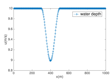
(a) Depth of water at initial time

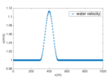
(b) Velocity of water at initial time

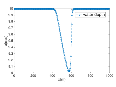
(c) Depth of water at end time

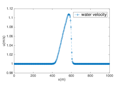
(d) Velocity of water at end time

Figure 5.1. Sampling results.

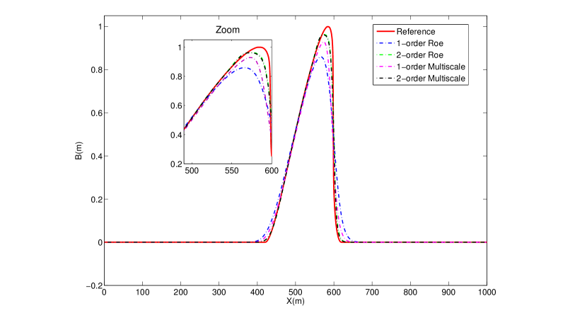
Figure 5.2. Comparison of different methods when $N=256$, $T=238079{\mathrm{s}}$.

5.1.2. Meyer-Peter-Müler Model

Figure 5.3 shows the comparison between Grass model and Meyer-Peter-Müler model when $u_{cr}=0.5$, $1.0$, and $1.04$. Here, all computations are carried out using the second order multi-scale algorithms, with parameters the same as above.

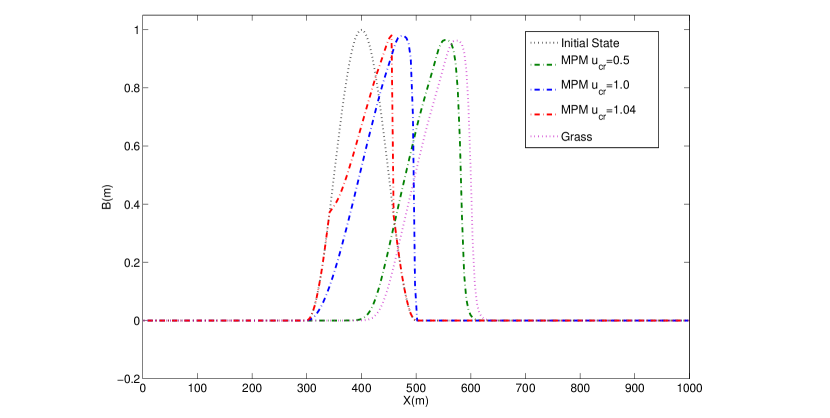
Figure 5.3. Comparison between Grass model and Meyer-Peter-Müler

5.1.3. Convergence results

Let us examine the convergence order of the multi-scale schemes. The test will be based on the Grass model. The Roe’s scheme [16, 17] on an extremely fine mesh with $16384$ grid points to is applied to produce the reference solution. Due to the limitation of our computing capacity, the computing time is comparatively short, says $T=90000{\mathrm{s}}$. Actually, the time $T=150/\varepsilon$ is enough for convergence order study. Here, we set $K=1$ and compute using both the first order and the second order algorithms. Besides, to study the effect of the $\mathcal{O}(\varepsilon)$ correction, we use the second order solver while discarding the $\mathcal{O}(\varepsilon)$ correction in the third test. The Table 1 shows the convergence order for each algorithm, $\hat{B}$ is the approximate solution and $B^{*}$ is the reference solution. One can see our algorithm has satisfactory convergence order, and the $\mathcal{O}(\varepsilon)$ correction is essential to improve the accuracy.

	first order		second order		without $\varepsilon$ correction
$N$	$\lVert\hat{B}-B^{*}\rVert_{1}$	order	$\lVert\hat{B}-B^{*}\rVert_{1}$	order	$\lVert\hat{B}-B^{*}\rVert_{1}$	order
128	7.05		3.22		3.24
256	3.68	0.94	1.03	1.65	1.05	1.63
512	1.88	0.97	3.25e-1	1.66	3.57e-1	1.55
1024	9.60e-1	0.97	9.01e-2	1.85	1.47e-1	1.27
2048	4.88e-1	0.97	2.39e-2	1.91	9.67e-2	0.61

Table 1. Convergence order of different algorithms.

5.1.4. Computing time comparison

We will show the computing times with different $A_{g}$’s and mesh sizes in this subsection. The ending time $T=150/\varepsilon$, the porosity constant is 0.4, and $K=2$ in the computations. For different cases that $A_{g}=0.01,0.005,0.001$ and $N=256,512$, Roe scheme, the first order multi-scale scheme and the second order multi-scale scheme are tested. From the computing times shown in the Table 2, we can see that for different $A_{g}$’s, the computing times of first order and second order scheme do not change a lot. It’s because the main computational cost attributes to solving the steady states, which does not change a lot for different $A_{g}$’s. These results demonstrate the efficiency of our multi-scale schemes, especially when $A_{g}$ is small enough.

$A_{g}$	$N$	Roe scheme	first order	second order
0.01	256	4.05	0.10	0.22
0.01	512	15.41	0.65	0.97
0.005	256	8.15	0.10	0.20
0.005	512	30.29	0.66	0.98
0.001	256	39.15	0.10	0.20
0.001	512	152.01	0.65	0.99

Table 2. Computing times (seconds) for different cases.

5.2. Two dimensional example

This example has been studied in [16, 17, 28]. We adopt the 2D case where the sediment transport takes place in a $1000m\times 1000m$ channel, with the initial dune profile as

(5.2) $$B(x,y,0)=\left\{\begin{array}[]{ll}\sin^{2}(\frac{(x-300)\pi}{200})\sin^{2}(\frac{(y-400)\pi}{200}),&\text{if}~{}300\leq x\leq 500,400\leq y\leq 600,\\ 0,&\text{else}.\end{array}\right.$$

The initial water surface level is $10$m everywhere with the uniformly horizontal discharge $Q=10m^{2}/s$, namely

$$h(x,y,0)=10-B(x,y,0),\quad u(x,y,0)=\frac{Q}{h(x,y,0)},\quad v(x,y,0)=0.$$

In this test, the Grass model with $m=3$ is used. The porosity is $0.4$ and time scaling parameter $\varepsilon=0.001/(1-0.4)$ to coincide with the model in [16].

When solving the steady state, we fix the discharge of $x$-direction to be $Q=10m^{2}/s$ at the upstream boundary, and the transmissive boundary condition is applied to the downstream boundary. The reflective boundary condition is adopted on the both sides of the channel. We also use the flux-limited Roe scheme [16, 17] to solve the steady state. As with 1D case, we solve the shallow water equations until the residual is less than $10^{-6}$ or the iteration number is bigger than 20000, and then the result is approximated to be the steady state. We compute this channel test problem using the second order multi-scale method until $T=3.6\times 10^{5}$s on a $128\times 128$ mesh. The CFL number is set to be $0.5$ and $K$ is set to be $2$. When solving the correction terms, we use the reflective boundary condition on the $y=0,1000m$, and use the zero boundaries condition on $x=0,1000m$. As with 1D case, the BiCGSTAB solver with SSOR preconditioner is used to solve the correction terms. The tolerance of the BiCGSTAB solver is $10^{-6}$ and the relaxation parameter of SSOR preconditioner is $0.955$.

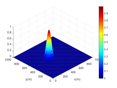
(a) Riverbed at initial time

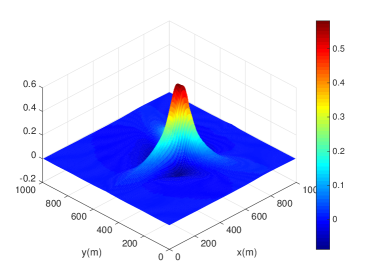
(b) Riverbed at end time

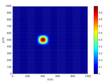
(c) Top view of riverbed at initial time

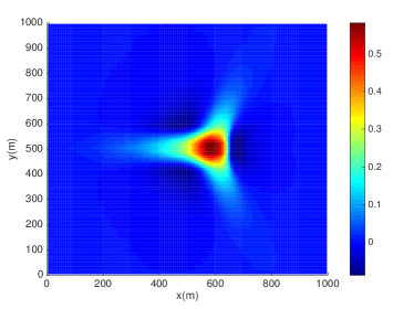
(d) Top view of riverbed at end time

Figure 5.4. Numerical results of riverbed.

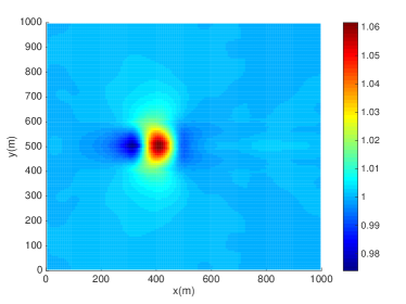
(a) Top view of $u$ at initial time

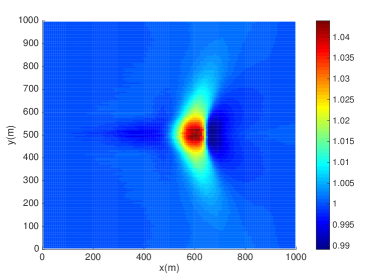
(b) Top view of $u$ at end time

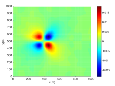
(c) Top view of $v$ at initial time

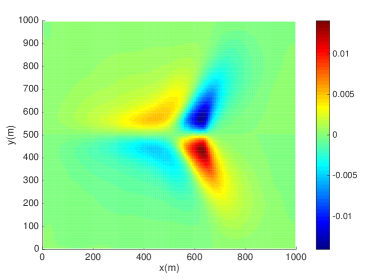
(d) Top view of $v$ at end time

Figure 5.5. Sampling results of water velocity.

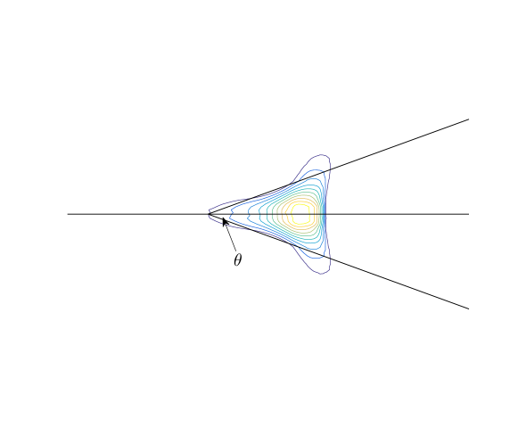
Figure 5.6. Spread angle.

Figure 5.4 shows the riverbed at initial time and end time. The steady state of velocities are shown in Figure 5.5. As shown in [16, 17, 28], the initial dune will gradually deform to a star-shaped pattern. From the Figure 5.4 one sees clearly that our method captures correctly such behaviors.

More precisely, the spread angle of the riverbed is important to show whether our model and scheme work [42, 43]. Assume that the interaction between the sediment layer and flow is low, the following approximation of the spread angle is proposed by De Vriend [43]

$$\tan\theta=\frac{3\sqrt{3}(m-1)}{9m-1}.$$

For the case in which $m=3$, the angle is approximately $21.78^{\circ}$. Figure 5.6 shows the contour of the riverbed at the ending time and also the angle $\theta=21.78^{\circ}$. From the figure, we observe that the spread angle of our scheme is very approximately to the one derived by De Vriend.

At last, the computing time of our multi-scale method is $492$s, which is much less than that of the flux-limited Roe’s method [16, 17] ($16806$s).

6. Conclusions

In this paper, a second order time homogenized model and the corresponding numerical methods for the sediment transport are proposed. Through the numerical experiments, the multi-scale method shows significant effectiveness, especially for the long time simulation of sediment transport while provides a considerably good approximation to the coupled system.

Appendix A Proofs of Lemma 1.1

Proof of Lemma 1.1.

Let $\lambda_{k}^{\varepsilon}=\lambda_{k}+\varepsilon\hat{\lambda}_{k}$ be the $k$-th eigenvalue of $\mathbf{C}^{\varepsilon}$. Then, we have

$$\big{[}(\mathbf{X}+\varepsilon\hat{\mathbf{X}})\mathbf{U}+(\mathbf{\Lambda}^{-1}\mathbf{X}\mathbf{g}+\varepsilon\hat{\mbox{\boldmath$\alpha$}})B\big{]}_{k}(x,t)$$

$$={} \big{[}(\mathbf{X}+\varepsilon\hat{\mathbf{X}})\mathbf{U}+(\mathbf{\Lambda}^{-1}\mathbf{X}\mathbf{g}+\varepsilon\hat{\mbox{\boldmath$\alpha$}})B\big{]}_{k}(x-\lambda_{k}^{\varepsilon}t,0).$$

Taking the spatial derivative to obtain

(A.1) $$\big{(}\mathbf{X}\mathbf{U}_{x}+\mathbf{\Lambda}^{-1}\mathbf{X}\mathbf{g}B_{x}\big{)}_{k}(x,t)=\big{(}\mathbf{X}\mathbf{U}_{x}+\mathbf{\Lambda}^{-1}\mathbf{X}\mathbf{g}B_{x}\big{)}_{k}(x-\lambda_{k}^{\varepsilon}t,0)$$

$$+\varepsilon\big{(}\hat{\mathbf{X}}\mathbf{U}_{x}+\hat{\mbox{\boldmath$\alpha$}}B_{x}\big{)}_{k}(x-\lambda_{k}^{\varepsilon}t,0)-\varepsilon\big{(}\hat{\mathbf{X}}\mathbf{U}_{x}+\hat{\mbox{\boldmath$\alpha$}}B_{x}\big{)}_{k}(x,t).$$

Since

$$\mathbf{X}\mathbf{U}_{x}+\mathbf{\Lambda}^{-1}\mathbf{X}\mathbf{g}B_{x}=\mathbf{\Lambda}^{-1}\mathbf{X}(\mathbf{A}\mathbf{U}_{x}+\mathbf{g}B_{x}),$$

and the initial state of fast variables, we get

$$\big{(}\mathbf{X}\mathbf{U}_{x}+\mathbf{\Lambda}^{-1}\mathbf{X}\mathbf{g}B_{x}\big{)}_{k}(x-\lambda_{k}^{\varepsilon}t,0)=\mathcal{O}(\varepsilon).$$

It follows from the boundedness of $\mathbf{U}_{x},B_{x}$ (one can check directly by the boundedness of $(\mathbf{K}^{\varepsilon})^{-1}$) that

$$\lVert\mathbf{X}\mathbf{U}_{x}+\mathbf{\Lambda}^{-1}\mathbf{X}\mathbf{g}B_{x}\rVert_{\infty}=\mathcal{O}(\varepsilon),$$

which implies

(A.2) $$\lVert\mathbf{A}\mathbf{U}_{x}+\mathbf{g}B_{x}\rVert_{\infty}=\mathcal{O}(\varepsilon)\quad\text{or}\quad\lVert\mathbf{U}_{\tau}\rVert_{\infty}=\mathcal{O}(1).$$

Let $E=B-B^{(0)}$. By subtracting (1.6) from (1.5), we have

$$E_{\tau}+\lambda^{(0)}_{B}E_{x}=\varepsilon\mathbf{c}^{T}\mathbf{A}^{-1}\mathbf{U}_{\tau}\qquad E(x,0)=0.$$

Thus,

$$E(x,\tau)=\varepsilon\int_{0}^{\tau}\mathbf{c}^{T}\mathbf{A}^{-1}\mathbf{U}_{\tau}(x-\lambda^{(0)}_{B}(\tau-s),s)\mathrm{d}s.$$

Finally, we have

$$\lVert E\rVert_{\infty}\leq C_{1}\varepsilon\int_{0}^{\tau}\lVert\mathbf{U}_{\tau}\rVert_{\infty}\mathrm{d}s\leq C_{2}\varepsilon\tau.$$

If $B(x,0)\in W^{2,\infty}(\mathbb{R})$, then we can take the spatial derivative again to (A.1) to obtain

(A.3) $$\big{(}\mathbf{X}\mathbf{U}_{xx}+\mathbf{\Lambda}^{-1}\mathbf{X}\mathbf{g}B_{xx}\big{)}_{k}(x,t)=\big{(}\mathbf{X}\mathbf{U}_{xx}+\mathbf{\Lambda}^{-1}\mathbf{X}\mathbf{g}B_{xx}\big{)}_{k}(x-\lambda_{k}^{\varepsilon}t,0)$$

$$+\varepsilon\big{(}\hat{\mathbf{X}}\mathbf{U}_{xx}+\hat{\mbox{\boldmath$\alpha$}}B_{xx}\big{)}_{k}(x-\lambda_{k}^{\varepsilon}t,0)-\varepsilon\big{(}\hat{\mathbf{X}}\mathbf{U}_{xx}+\hat{\mbox{\boldmath$\alpha$}}B_{xx}\big{)}_{k}(x,t),$$

which yields

$$\|\mathbf{A}\mathbf{U}_{xx}+\mathbf{g}B_{xx}\|_{\infty}=\mathcal{O}(\varepsilon),\quad\text{or}\quad\|\mathbf{U}_{\tau x}\|_{\infty}=\mathcal{O}(\varepsilon),$$

by the similar argument. Then

$$(E_{x})_{\tau}+\lambda_{B}^{(0)}(E_{x})_{x}=\varepsilon\mathbf{c}^{T}\mathbf{A}^{-1}\mathbf{U}_{\tau x}\qquad E_{x}(x,0)=0,$$

which means that

$$\|E_{x}\|_{\infty}\leq C_{1}\varepsilon\int_{0}^{\tau}\|\mathbf{U}_{\tau x}\|_{\infty}{\mathrm{d}}s\leq C_{2}\varepsilon\tau.$$

This ends the proof. ∎

Appendix B Proof of Lemma 1.2

Proof of Lemma 1.2.

From (1.4), we have

$$\mathbf{K}^{\varepsilon}\mathbf{C}^{\varepsilon}=\mathbf{D}^{\varepsilon}\mathbf{K}^{\varepsilon},$$

which can be written as

$$\begin{pmatrix}\mathbf{X}+\varepsilon\hat{\mathbf{X}}&\mathbf{\Lambda}^{-1}\mathbf{X}\mathbf{g}+\varepsilon\hat{\mbox{\boldmath$\alpha$}}\\ \varepsilon\hat{\mbox{\boldmath$\beta$}}^{T}&1+\varepsilon\hat{\theta}\end{pmatrix}\begin{pmatrix}\mathbf{A}&\mathbf{g}\\ \varepsilon\mathbf{c}^{T}&0\end{pmatrix}=\begin{pmatrix}\mathbf{\Lambda}+\varepsilon\hat{\mathbf{\Lambda}}&0\\ 0&\varepsilon\mu\end{pmatrix}\begin{pmatrix}\mathbf{X}+\varepsilon\hat{\mathbf{X}}&\mathbf{\Lambda}^{-1}\mathbf{X}\mathbf{g}+\varepsilon\hat{\mbox{\boldmath$\alpha$}}\\ \varepsilon\hat{\mbox{\boldmath$\beta$}}^{T}&1+\varepsilon\hat{\theta}\end{pmatrix}.$$

By expanding this equation, we have

$$(\mathbf{X}+\varepsilon\hat{\mathbf{X}})\mathbf{A}+\varepsilon(\mathbf{\Lambda}^{-1}\mathbf{X}\mathbf{g}+\varepsilon\hat{\mbox{\boldmath$\alpha$}})\mathbf{c}^{T} =(\mathbf{\Lambda}+\varepsilon\hat{\mathbf{\Lambda}})(\mathbf{X}+\varepsilon\hat{\mathbf{X}}),$$

$$(\mathbf{X}+\varepsilon\hat{\mathbf{X}})\mathbf{g} =(\mathbf{\Lambda}+\varepsilon\hat{\mathbf{\Lambda}})(\mathbf{\Lambda}^{-1}\mathbf{X}\mathbf{g}+\varepsilon\hat{\mbox{\boldmath$\alpha$}}).$$

By collecting the $\mathcal{O}(\varepsilon)$ term we have

$$\left\{\begin{aligned} \hat{\mathbf{X}}\mathbf{g}&=\mathbf{\Lambda}\hat{\mbox{\boldmath$\alpha$}}+\hat{\mathbf{\Lambda}}\mathbf{\Lambda}^{-1}\mathbf{X}\mathbf{g}+\mathcal{O}(\varepsilon),\\ \hat{\mathbf{X}}\mathbf{A}+\mathbf{\Lambda}^{-1}\mathbf{X}\mathbf{g}\mathbf{c}^{T}&=\mathbf{\Lambda}\hat{\mathbf{X}}+\hat{\mathbf{\Lambda}}\mathbf{X}+\mathcal{O}(\varepsilon).\end{aligned}\right.$$

Or

(B.1) $$\left\{\begin{aligned} \hat{\mbox{\boldmath$\alpha$}}&=\mathbf{\Lambda}^{-1}\hat{\mathbf{X}}\mathbf{g}-\hat{\mathbf{\Lambda}}\mathbf{\Lambda}^{-2}\mathbf{X}\mathbf{g}+\mathcal{O}(\varepsilon),\\ \mathbf{\Lambda}^{-1}\mathbf{X}\mathbf{g}\mathbf{c}^{T}&=\mathbf{\Lambda}\hat{\mathbf{X}}+\hat{\mathbf{\Lambda}}\mathbf{X}-\hat{\mathbf{X}}\mathbf{X}^{-1}\mathbf{\Lambda}\mathbf{X}+\mathcal{O}(\varepsilon).\end{aligned}\right.$$

In light of the proof of Lemma 1.1, it suffices to show that

(B.2) $$\lVert\mathbf{U}^{(1)}_{\tau}-\mathbf{U}_{\tau}\rVert_{\infty}=\mathcal{O}(\varepsilon).$$

Note that $\mathbf{U}^{(1)}$ and $B^{(0)}$ satisfy

(B.3) $$\begin{pmatrix}\mathbf{U}^{(1)}\\ B^{(0)}\\ \end{pmatrix}_{t}+\begin{pmatrix}\mathbf{A}&\mathbf{g}\\ 0&-\varepsilon\mathbf{c}^{T}\mathbf{A}^{-1}\mathbf{g}\\ \end{pmatrix}\begin{pmatrix}\mathbf{U}^{(1)}\\ B^{(0)}\\ \end{pmatrix}_{x}=0.$$

Let

$$\mathbf{C}_{1}^{\varepsilon}=\begin{pmatrix}\mathbf{A}&\mathbf{g}\\ 0&-\varepsilon\mathbf{c}^{T}\mathbf{A}^{-1}\mathbf{g}\\ \end{pmatrix}.$$

Again by the perturbation theory [35], $\mathbf{C}^{\varepsilon}_{1}$ has the following decomposition

(B.4) $$\mathbf{C}^{\varepsilon}_{1}=(\mathbf{K}^{\varepsilon}_{1})^{-1}\mathbf{D}_{1}^{\varepsilon}\mathbf{K}^{\varepsilon}_{1},$$

where

$$\mathbf{K}^{\varepsilon}_{1}=\begin{pmatrix}\mathbf{X}+\varepsilon\hat{\mathbf{X}}_{1}&\mathbf{\Lambda}^{-1}\mathbf{X}\mathbf{g}+\varepsilon\hat{\mbox{\boldmath$\alpha$}}_{1}\\ \varepsilon\hat{\mbox{\boldmath$\beta$}}_{1}^{T}&1+\varepsilon\hat{\theta}_{1}\end{pmatrix}\qquad\mathbf{D}_{1}^{\varepsilon}=\begin{pmatrix}\mathbf{\Lambda}&0\\ 0&-\varepsilon\mathbf{c}^{T}\mathbf{A}^{-1}\mathbf{g}\\ \end{pmatrix}.$$

Collecting the $\mathcal{O}(\varepsilon)$ terms in (B.4), we have

(B.5) $$\hat{\mathbf{X}}_{1}=\mathbf{X}\qquad\mathbf{\Lambda}\hat{\mbox{\boldmath$\alpha$}}_{1}=\mathbf{X}\mathbf{g}-\mathbf{\Lambda}^{-1}\mathbf{X}\mathbf{g}\mathbf{c}^{T}\mathbf{X}^{-1}\mathbf{\Lambda}^{-1}\mathbf{X}\mathbf{g}\qquad\hat{\mbox{\boldmath$\beta$}}_{1}=\mathbf{0}.$$

Comparing with (A.1) in Lemma 1.1, and from (B.5) and the initial condition, we have

$$\left[\mathbf{X}(\mathbf{U}-\mathbf{U}^{(1)})_{x}+\mathbf{\Lambda}^{-1}\mathbf{X}\mathbf{g}(B-B^{(0)})_{x}\right]_{k}(x,t)$$

$$={} \left[(\mathbf{X}+\varepsilon\hat{\mathbf{X}})\mathbf{U}_{x}+(\mathbf{\Lambda}^{-1}\mathbf{X}\mathbf{g}+\varepsilon\hat{\mbox{\boldmath$\alpha$}})B_{x}\right]_{k}(x-\lambda_{k}^{\varepsilon}t,0)$$

$$-\left[(\mathbf{X}+\varepsilon\hat{\mathbf{X}}_{1})\mathbf{U}^{(1)}_{x}+(\mathbf{\Lambda}^{-1}\mathbf{X}\mathbf{g}+\varepsilon\hat{\mbox{\boldmath$\alpha$}}_{1})B^{(0)}_{x}\right]_{k}(x-\lambda_{k}t,0)$$

$$-\varepsilon(\hat{\mathbf{X}}\mathbf{U}_{x}+\hat{\mbox{\boldmath$\alpha$}}B_{x})_{k}(x,t)+\varepsilon(\hat{\mathbf{X}}_{1}\mathbf{U}^{(1)}_{x}+\hat{\mbox{\boldmath$\alpha$}}_{1}B_{x}^{(0)})_{k}(x,t)+\mathcal{O}(\varepsilon^{2})$$

$$={} -\varepsilon(\hat{\mathbf{X}}\mathbf{U}_{x}+\hat{\mbox{\boldmath$\alpha$}}B_{x})_{k}(x,t)+\varepsilon\hat{\mathbf{X}}_{1}\mathbf{U}^{(1)}_{x}+\hat{\mbox{\boldmath$\alpha$}}_{1}B_{x}^{(0)})_{k}(x,t)+\mathcal{O}(\varepsilon^{2})$$

$$={} \varepsilon(\mathbf{X}\mathbf{U}_{x}^{(1)}+\mathbf{\Lambda}^{-1}\mathbf{X}\mathbf{g}B_{x}^{(0)})_{k}(x,t)+\varepsilon(\mathbf{\Lambda}^{-2}\mathbf{X}\mathbf{g}\mathbf{c}^{T}\mathbf{X}^{-1}\mathbf{\Lambda}^{-1}\mathbf{X}\mathbf{g})_{k}(B_{x}-B_{x}^{(0)})(x,t)$$

$$-\varepsilon\left[\hat{\mathbf{X}}\mathbf{U}_{x}+(\hat{\mbox{\boldmath$\alpha$}}+\mathbf{\Lambda}^{-2}\mathbf{X}\mathbf{g}\mathbf{c}^{T}\mathbf{X}^{-1}\mathbf{\Lambda}^{-1}\mathbf{X}\mathbf{g})B_{x}\right]_{k}(x,t)+\mathcal{O}(\varepsilon^{2})$$

By the similar technique as Lemma 1.1, we can prove

$$\|\mathbf{X}\mathbf{U}_{x}^{(1)}+\mathbf{\Lambda}^{-1}\mathbf{X}\mathbf{g}B_{x}^{(0)}\|_{\infty}=\mathcal{O}(\varepsilon).$$

And Lemma 1.1 proves that $\|B_{x}-B_{x}^{(0)}\|_{\infty}=\mathcal{O}(\varepsilon)$. In light of the (B.1), we have the following estimate for the last part:

$$\hat{\mathbf{X}}\mathbf{U}_{x}+(\hat{\mbox{\boldmath$\alpha$}}+\mathbf{\Lambda}^{-2}\mathbf{X}\mathbf{g}\mathbf{c}^{T}\mathbf{X}^{-1}\mathbf{\Lambda}^{-1}\mathbf{X}\mathbf{g})B_{x}$$

$$={} \hat{\mathbf{X}}\mathbf{A}^{-1}(\mathbf{A}\mathbf{U}_{x}+\mathbf{g}B_{x})+(\hat{\mbox{\boldmath$\alpha$}}+\mathbf{\Lambda}^{-2}\mathbf{X}\mathbf{g}\mathbf{c}^{T}\mathbf{X}^{-1}\mathbf{\Lambda}^{-1}\mathbf{X}\mathbf{g}-\hat{\mathbf{X}}\mathbf{X}^{-1}\mathbf{\Lambda}^{-1}\mathbf{X}\mathbf{g})B_{x}$$

$$={} \mathbf{\Lambda}^{-1}(\hat{\mathbf{X}}-\mathbf{\Lambda}^{-1}\hat{\mathbf{\Lambda}}\mathbf{X}+\mathbf{\Lambda}^{-1}\mathbf{X}\mathbf{g}\mathbf{c}^{T}\mathbf{X}^{-1}\mathbf{\Lambda}^{-1}\mathbf{X}-\mathbf{\Lambda}\hat{\mathbf{X}}\mathbf{X}^{-1}\mathbf{\Lambda}^{-1}\mathbf{X})\mathbf{g}B_{x}+\mathcal{O}(\varepsilon)$$

$$={} \mathbf{\Lambda}^{-1}\left[\hat{\mathbf{X}}-\mathbf{\Lambda}^{-1}\hat{\mathbf{\Lambda}}\mathbf{X}+(\mathbf{\Lambda}\hat{\mathbf{X}}+\hat{\mathbf{\Lambda}}\mathbf{X}-\hat{\mathbf{X}}\mathbf{A})\mathbf{X}^{-1}\mathbf{\Lambda}^{-1}\mathbf{X}-\mathbf{\Lambda}\hat{\mathbf{X}}\mathbf{X}^{-1}\mathbf{\Lambda}^{-1}\mathbf{X}\right]\mathbf{g}B_{x}+\mathcal{O}(\varepsilon)$$

$$={} \mathcal{O}(\varepsilon).$$

Here, we have used the fact that $\hat{\mathbf{\Lambda}}$ is diagonal. From the above, we finally obtain

$$\lVert\mathbf{X}(\mathbf{U}-\mathbf{U}^{(1)})_{x}+\mathbf{\Lambda}^{-1}\mathbf{g}(B-B^{(0)})_{x}\rVert_{\infty}=\mathcal{O}(\varepsilon^{2}),$$

which implies that

$$\lVert\mathbf{A}(\mathbf{U}-\mathbf{U}^{(1)})_{x}+\mathbf{g}(B-B^{(0)})_{x}\rVert_{\infty}=\mathcal{O}(\varepsilon^{2}).$$

Thus, we have

$$\lVert\mathbf{U}_{\tau}-\mathbf{U}^{(1)}_{\tau}\rVert_{\infty}=\mathcal{O}(\varepsilon).$$

This completes the proof. ∎

References

[1]
Peter R Wilcock, John Pitlick, Yantao Cui, et al.
Sediment transport primer: estimating bed-material transport in
gravel-bed rivers.
2009.
[2]
J.A. Cunge, F.M. Holly, and A. Verwey.
Practical aspects of computational river hydraulics.
Pitman, 1980.
[3]
Daryl B Simons and Fuat Şentürk.
Sediment transport technology: water and sediment dynamics.
Water Resources Publication, 1992.
[4]
A.J. Grass.
Sediment transport by waves and currents.
SERC London Centre for Marine Technology, Report No. FL29,
1981.
[5]
E. Meyer-Peter and R. Müller.
Formulas for bed-load transport.
In Proceedings of the 2nd Meeting of the International
Association for Hydraulic Structures Research, pages 39–64. Stockholm,
1948.
[6]
R Fernandez Luque and R Van Beek.
Erosion and transport of bed-load sediment.
Journal of Hydraulic Research, 14(2):127–144, 1976.
[7]
L.C. Van Rijn.
Sediment transport, part I: bed load transport.
Journal of Hydraulic Engineering, 110(10):1431–1456, 1984.
[8]
L.C. Van Rijn.
Principles of sediment transport in rivers, estuaries and
coastal seas, volume 1006.
Aqua publications Amsterdam, 1993.
[9]
P. Nielsen.
Coastal bottom boundary layers and sediment transport,
volume 4.
World scientific, 1992.
[10]
Benoît Camenen and Magnus Larson.
A general formula for non-cohesive bed load sediment transport.
Estuarine, Coastal and Shelf Science, 63(1):249–260, 2005.
[11]
Felix M Exner.
Zur physik der dünen.
Akad. Wiss. Wien Math. Naturwiss. Klasse, 129(2a):929–952,
1920.
[12]
Felix M Exner.
Uber die wechselwirkung zwischen wasser und geschiebe in flüssen.
Akad. Wiss. Wien Math. Naturwiss. Klasse, 134(2a):165–204,
1925.
[13]
R. Soulsby.
Dynamics of marine sands: a manual for practical applications.
Thomas Telford, 1997.
[14]
W. Wu.
Computational river dynamics.
CRC Press, 2008.
[15]
C Juez, J Murillo, and P García-Navarro.
A 2d weakly-coupled and efficient numerical model for transient
shallow flow and movable bed.
Advances in Water Resources, 71:93–109, 2014.
[16]
J. Hudson.
Numerical techniques for morphodynamic modelling.
PhD thesis, University of Reading, 2001.
[17]
J. Hudson, J. Damgaard, N. Dodd, T. Chesher, and A. Cooper.
Numerical approaches for 1D morphodynamic modelling.
Coastal engineering, 52(8):691–707, 2005.
[18]
Stéphane Cordier, Minh H Le, and T Morales de Luna.
Bedload transport in shallow water models: Why splitting (may) fail,
how hyperbolicity (can) help.
Advances in Water Resources, 34(8):980–989, 2011.
[19]
J. Hudson and P.K. Sweby.
Formulations for numerically approximating hyperbolic systems
governing sediment transport.
Journal of Scientific Computing, 19(1-3):225–252, 2003.
[20]
J. Hudson and P.K. Sweby.
A high-resolution scheme for the equations governing 2D bed-load
sediment transport.
International Journal for Numerical Methods in Fluids,
47(10-11):1085–1091, 2005.
[21]
MJ Castro Dı, Enrique D Fernández-Nieto, AM Ferreiro, C Parés,
et al.
Two-dimensional sediment transport models in shallow water equations.
a second order finite volume approach on unstructured meshes.
Computer Methods in Applied Mechanics and Engineering,
198(33):2520–2538, 2009.
[22]
Javier Murillo and P García-Navarro.
An exner-based coupled model for two-dimensional transient flow over
erodible bed.
Journal of Computational Physics, 229(23):8704–8732, 2010.
[23]
T Morales De Luna, MJ Castro Díaz, and C Parés Madronal.
A duality method for sediment transport based on a modified
meyer-peter & müller model.
Journal of Scientific Computing, 48(1-3):258–273, 2011.
[24]
Alberto Serrano-Pacheco, Javier Murillo, and Pilar Garcia-Navarro.
Finite volumes for 2d shallow-water flow with bed-load transport on
unstructured grids.
Journal of Hydraulic Research, 50(2):154–163, 2012.
[25]
L. Fracarollo, H. Capart, and Zech Y.
A Godunov method for the computation of erosional Shallow Water
transients.
International Journal for Numerical Methods in Fluids,
41:951–976, 2003.
[26]
Nelida Črnjarić Žic, Senka Vuković, and Luka Sopta.
Balanced finite volume weno and central weno schemes for the shallow
water and the open-channel flow equations.
J. Comput. Phys., 200(2):512–548, November 2004.
[27]
M.J. Castro Diaz, E.D. Fernández-Nieto, and A.M. Ferreiro.
Sediment transport models in shallow water equations and numerical
approach by high order finite volume methods.
Computers & Fluids, 37(3):299–316, 2008.
[28]
A.I. Delis and I. Papoglou.
Relaxation approximation to bed-load sediment transport.
Journal of Computational and Applied Mathematics,
213(2):521–546, 2008.
[29]
F. Benkhaldoun, S. Sahmim, and M. Seaid.
Solution of the sediment transport equations using a finite volume
method based on sign matrix.
SIAM Journal on Scientific Computing, 31(4):2866–2889, 2009.
[30]
Matteo Postacchini, Maurizio Brocchini, Alessandro Mancinelli, and Marc Landon.
A multi-purpose, intra-wave, shallow water hydro-morphodynamic
solver.
Advances in Water Resources, 38:13–26, 2012.
[31]
R Briganti, N Dodd, D Kelly, and D Pokrajac.
An efficient and flexible solver for the simulation of the
morphodynamics of fast evolving flows on coarse sediment beaches.
International Journal for Numerical Methods in Fluids,
69(4):859–877, 2012.
[32]
Marco Bilanceri, François Beux, Imad Elmahi, Hervé Guillard, and
Maria Vittoria Salvetti.
Linearized implicit time advancing and defect correction applied to
sediment transport simulations.
Computers & Fluids, 63:82–104, 2012.
[33]
M. De Vries.
River-bed variations-aggradation and degradation.
I.H.A.R. International Seminar on Hydraulics of Alluvial Streams, New
Dehli, 1973.
[34]
Weinan E and Bjorn Engquist.
The heterogeneous multiscale methods.
Communications in Mathematical Sciences, 1(1):88–134, 2003.
[36]
Derek S. Bale, Randall J. Leveque, Sorin Mitran, and James A. Rossmanith.
A wave propagation method for conseration laws and balance laws with
spatially varing flux functions.
SIAM Journal on Scientific Computing, 24(3):995–978, 2002.
[37]
A. Harten.
High resolution schemes for hyperbolic conservation laws.
Journal of Computaional Physics, 49(3):357–393, 1983.
[38]
S. Gottlieb and C.-W. Shu.
Total varation diminishing Runge-Kutta schemes.
Mathematics of Computation, 67(221):73–85, 1998.
[39]
B. van Leer.
Towars the ultimate conserative difference scheme. \@slowromancapv@. A
second-order sequeal to Godunov’s method.
Journal of Computational Physics, 32:101–136, 1979.
[40]
K.H. Kim and Chongam Kim.
Accurate, efficient and monotonic numerical methods for
multidimensional compressible flows: Part \@slowromancapii@ : Multi-dimensional
limiting process.
Journal of Computaional Physics, 208:570–615, 2005.
[41]
J. Deng, R. Li, T. Sun, and S.-N. Wu.
Robust a simulation for shallow flows with friction on rough
topography.
Numerical Mathematics: Theory, Methods and Applications,
6(2):384–407, 2013.
[42]
Jean de Dieu Zabsonré, Carine Lucas, and Enrique Fernandez-Nieto.
An energetically consistent viscous sedimentation model.
Mathematical Models and Methods in Applied Sciences,
19(03):477–499, 2009.
[43]
HJ (nd) De Vriend.
2dh mathematical modelling of morphological evolutions in shallow
water.
Coastal Engineering, 11(1):1–27, 1987.