Cooperative peer-to-peer multiagent based systems

Abstract

A multiagent based model for a system of cooperative agents aiming at growth is proposed. This is based on a set of generalized Verhulst-Lotka-Volterra differential equations. In this study, strong cooperation is allowed among agents having similar sizes, and weak cooperation if agent have markedly different “sizes”, thus establishing a peer-to-peer modulated interaction scheme. A rigorous analysis of the stable configurations is presented first examining the fixed points of the system, next determining their stability as a function of the model parameters. It is found that the agents are self-organizing into clusters. Furthermore, it is demonstrated that, depending on parameter values, multiple stable configurations can coexist. It occurs that only one of them always emerges with probability close to one, because its associated attractor dominates over the rest. This is shown through numerical integrations and simulations,after analytic developments. In contrast to the competitive case, agents are able to increase their capacity beyond the no-interaction case limit. In other words, when some collaborative partnership among a relatively small number of partners takes place, all agents act in good faith prioritizing the common good, whence receiving a mutual benefit allowing them to surpass their capacity.

I Introduction

It is usually accepted that the fittest survive through natural selection Darwin . The former biological feature has been extended to social and moral concepts. It should be recalled that Darwin’s conclusion pertained to the preservation of favored races in the struggle for life, when species performed in a given environment. However, the question of species competition $or$ cooperation among themselves for survival is another matter.

Generally speaking, species social systems are in fact classified in competitive, cooperative or mixed type, depending on the set of interactions existing among agents. For example, in Nature, ants exhibit a typical cooperative behavior dorigo2004ant ; ANTS , on the other side, in economy, companies sharing a customer market usually behave as natural competitors fehr1999theory . However, collaboration with competitors might be a winning strategy hamel1989collaborate ; rey2013cooperation ; luo2006cross ; hauert2006cooperation ; doi:10.1142/S0219525912500592 ; doi:10.1142/S0219525913500367 .

Thus, fundamental, beside moral or economic, questions can be raised about sets of interacting agents exhibiting emergence of a self-organizing collective behavior, not resulting from the existence of a“central controller” boccara2004modeling ; bar1997dynamics ; Knyazeva ; porter2000location , but due to their own interactions with the other agents.

Several simulation and analytic studies can be found in the literature on such systems, called prey-predator models. However, for such systems, the agent interacting processes can be also modeled by using a set of ordinary differential equations (ODEs), for example, following a Lotka-Volterra (LV) model boccara2004modeling ; Lotka ; Volterra . The time evolution or dynamics of the system can be displayed along a continuous time axis, rather than at discrete time points, in simulation work.

For example, in Huberman ; Huberman2 the LV model was used to model the competition among websites using constant and equal interactions among all agents. It was found that two distinctive behaviors are possible: winner takes all and sharing the market. In Yanhui , this model was modified by introducing a non-constant and linear interaction which allows the emergence of the rich gets richer behavior. Moreover, in Caram , a competitive $non-linear$ interaction was considered leading to a stratification or clustering of agents, as often observed in economic life.

In this work, a cooperative scenario between agents, rather than a competitive one, is presented, based on a similar set of LV model differential equations. Particularly, how the “size” of the each agent increases (or not) is studied depending on the cooperation with the other agents. When modelling such a socio-economic multi agent system, the “size” is understood as something similar to the market share, Huberman ; Yanhui ; Caram . In this line of thought, the $n$ interacting agents are all needing some common resources within a general environment. Here below, an interaction function is introduced, which allows agents to cooperate in a selective way, i.e. the interaction is strong between those agents with similar or equal sizes. On the other hand, a weaker cooperative interaction is between agents if they have very different sizes. As a side way argument, it can be considered that such a same-size-cooperative rule occurs in sport competition. For example, the main (soccer) teams share the best players in order to remain at the top.

Here, a simple symmetric model is considered, i.e. by assuming that the strength of cooperation is reciprocal between two cooperating agents. It is shown that this model allows for unvealing the main features of this interesting type of systems. More sophisticated interactions including, for example, asymmetry in the cooperation could be addressed in the future as an extension of this wok (see section VI). Therefore, here our cooperative system has two parameters, $\sigma$ and $K$, (see equation (5) in Section II):

• (a) $\sigma$ scales the difference between agent sizes,

• (b) $K$ defines the kind of scenario (cooperative or not) and also controls the amplitude of the interactions.

The main purpose of this paper is to analyze the cooperative scenario and demonstrate that a synergy is established leading to a situation in which every interacting agent is benefited from the group. This is the point that makes the difference with other previous works Huberman ; Yanhui ; Caram .

This paper is organized as follows: in Section II, the mathematical model is described; in Section III, the cooperative scenario is studied in detail; in Section IV, the fixed points are searched and the $K$ parameter range effect is analysed; in Section V, simulations and results for a case of ten agents are shown; finally, in Section VI, the main conclusions are outlined.

II The model

Let $n$ agents be sharing some common resource; when an agent is able to get some portion of the common resource, its size increases, but if losing a portion of its resource its size decreases. In the model, essentially based on the well known prey-predator model, the interaction parameter is not assumed to be a constant: it is supposed to depend on the difference between agent sizes. This fact implies that sizes do dynamically change in time, expectedly producing a highly complex dynamics, - due to a feedback phenomenon. Mathematically, the model is based on Verhulst evolution equations Verhulst1 ; Verhulst2

$$\dot{s}_{i}=\alpha_{i}s_{i}\left(\beta_{i}-s_{i}\right),$$ (1)

and on the generalized Lotka-Volterra evolution equations Lotka ; Volterra

$$\dot{s}_{i}=\alpha_{i}s_{i}\left(\beta_{i}-s_{i}\right)-{\sum\limits_{i\neq j}}\gamma_{ij}s_{i}s_{j},\mbox{ \ \ \ \ \ \ for \ \ \ \ }i\neq j,\mbox{ \ \ \ \ \ \ and \ \ \ \ }i=1,\dots,n$$ (2)

where $s_{i}$ is the size of agent $i$, $\alpha_{i}$ is the agent’s growth rate, $\beta_{i}$ is the agent’s maximum capacity and $\gamma_{ij}$ is a constant coefficient determining the interaction between $s_{i}$ and $s_{j}$. Eq.(2) is easily generalized to read

$$\dot{s}_{i}=\alpha_{i}s_{i}\left(\beta_{i}-s_{i}\right)-{\sum\limits_{i\neq j}}\gamma\left(s_{i},s_{j}\right)s_{i}s_{j},\mbox{ \ \ \ \ \ \ for \ \ \ \ }i=1,\dots,n,$$ (3)

where $\gamma\left(s_{i},s_{j}\right)$ is the interaction between agent $s_{i}$ and agent $s_{j}$, here this matrix is composed by dynamic parameters that result from the difference between both agent sizes in relation. There is no time lag delay. Therefore, each agent size $s_{i}(t)$ represents a portion of common resource that the agent is able to get at a given time $t$. When the interaction $\gamma\left(s_{i},s_{j}\right)\neq 0$, a feedback situation is present; if $\gamma=0$ the system is reduced to the basic uncoupled LV / Kolmogorov prey-predator model Lotka ; Volterra . In this case, each agent size grows according to its particular rate $\alpha_{i}$, up to its maximum capacity $\beta_{i}$ or its possible maximum size, as it happens in the population dynamics model of Verhulst Verhulst1 ; Verhulst2 .

Thereafter, the interaction function $\gamma\left(s_{i},s_{j}\right)$ is supposed to be non linear, symmetric, and monotonically decreasing with distance from its centre Caram ; broomhead1988radial

$$\gamma\left(s_{i},s_{j}\right)=K\exp\left[-\left(\frac{s_{i}-s_{j}}{\sigma}\right)^{2}\right],$$ (4)

where $\sigma>0$, is a positive (kernel bandwidth) parameter that controls or scales the size similarity i.e. it regulates the difference in size of agents and determines the interaction levels. On the other hand, $K$ determines the type of scenario: $K>0$ (competitive case, as studied in Caram ), or $K<0$ (cooperative case), as studied here below. The absolute value $|K|$ defines the amplitude of the interaction. Therefore, the dynamics is dominated by the interaction which can be “strong” or “weak” depending on the sizes of agents. It seems obvious that when a big agent is interacting with a small one, the intensity of their interaction is weak or almost null, since their “size distance” is large. A contrario, when two agents with the same or similar sizes are interacting, the intensity of their interaction can be very strong. It is easy to see from Eq.(4) that $\gamma\left(s_{i},s_{j}\right)$ varies between $0$ and $K$.

It is not too difficult to conserve a full set of different $\alpha_{i}$ and $\beta_{i}$, characterising each agent. However, the writing is much more heavy if doing so. In order to remain within the purpose of this paper, it is advantageous to consider that all agents have the same basic dynamics properties. This is equivalent to rescaling the various sizes and the time scales. Thus, thereafter, let $\alpha_{i}=1$ and $\beta_{i}=1$. The whole model becomes:

$$\dot{s}_{i}=s_{i}\left(1-s_{i}\right)-{\sum\limits_{i\neq j}}K\exp\left[{-\left(\frac{s_{i}-s_{j}}{\sigma}\right)^{2}}\right]s_{i}s_{j}.$$ (5)

III Detailed analysis of the cooperative scenario

A cooperative scenario occurs when $K$ is negative in Eq.(5), i.e. creating a positive feedback. Instead of stabilizing the system, this leads to very unstable and complex behaviors. Therefore, the various interesting values of $K$, must be chosen carefully. It will be seen in section IV.1, that this choice depends on the total number of agents which are cooperating. This analysis will show that there is a quite limited range of $K$ values such that the model system reaches a stable behavior in the steady state.

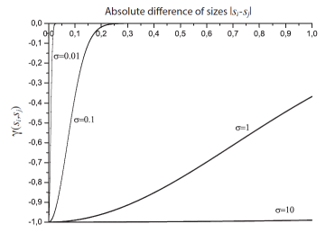
Figure 1: Interaction function $\gamma$ vs. absolute difference of sizes $|s_{i}-s_{j}|$, for different scaling similarity parameter $\sigma$ values and for $K=-1$.

First, it is obvious that cooperation is at its maximum and equal to $K$, when $s_{i}=s_{j}$, because of the definition of $\gamma\left(s_{i},s_{j}\right)$. The possible variation range of $\gamma\left(s_{i},s_{j}\right)$ is shown in Figure 1, as a function of the difference in sizes, for different values of $\sigma$. As can be seen in this figure, when the (absolute) difference in sizes increases, the cooperation decreases: $\gamma\left(s_{i},s_{j}\right)$ becomes less negative; its possible values all within the range $-K<\gamma\left(s_{i},s_{j}\right)<0$. It is clear that, for example when $\sigma=10$ and $\left|s_{i}-s_{j}\right|<1$, the cooperation is almost constant and equal to $\gamma_{ij}\left(s_{i},s_{j}\right)=-K$. When $\sigma\rightarrow\ 0$, the interaction function looks like an inverted Dirac distribution, at the origin.

In the following Section IV, it is shown how a narrow and limited range of $K$ values, for different number of agents, leads the system to stable configurations in the steady stationary state. The emergence of different behaviors will be also shown, i.e. the formation of clusters of agents whose sizes are larger than their limit, i.e. its maximum capacity ($\beta_{i}=1$) in absence of interaction. More interestingly, the coexistence of several stable configurations is proved analytically and validated by numerical simulations.

IV Analysis of fixed points and range of parameter $K$

By definition, a fixed point (FP) is a point in the phase space where all the time derivatives are zero, i.e.,

$$\dot{s}_{i}=0,\mbox{ \ \ \ \ \ \ for \ \ \ \ }i=1,\dots,n.$$ (6)

For the stability analysis associated to every fixed point, one looks at the eigenvalues of the Jacobian matrix $J$ evaluated at the corresponding FP. It is rather easily derived that the Jacobian matrix elements are:

$$\left[J\right]_{\left(i,k\right)}=\frac{\partial\dot{s}_{i}}{\partial s_{k}}=\left\{\begin{array}[]{ll}1-2s_{i}-{\sum\limits_{i\neq j}}s_{j}\gamma\left(s_{i},s_{j}\right)\left[1-\frac{2}{\sigma^{2}}s_{i}\left(s_{i}-s_{j}\right)\right],&\mbox{\ \ for \ }k=i,\\ -s_{i}\gamma\left(s_{i},s_{k}\right)\left[1+\frac{2}{\sigma^{2}}s_{k}\left(s_{i}-s_{k}\right)\right],&\mbox{\ \ for \ }k\neq i.\end{array}\right.$$ (7)

IV.1 Trivial fixed points for an arbitrary number $n$ of agents

In this section, the existence of fixed points and their stability analysis are presented when the number of agents allows some analytical work.

From equations (5) and (6), at least three trivial FP can be detected:

• (I) $s_{i}=0$,                     for     $i=1,\dots,n$ ,
  i.e. all agents have zero size;

• (II) $s_{i}=1$ and $s_{j}=0$,     for every     $j\neq i$ ,
  i.e. all agents have zero size, except one;

• (III) $s_{i}=b$,                     for     $i=1,\dots,n$ ,
  i.e. all agents have the same size $b$.

In addition to the type (I), (II) and (III) FP, there are many other points that verify the condition of a fixed point. These points are found by numerically seeking the roots of the non-linear Eq. (6); see Sect. IV.2.

If the Jacobian matrix is evaluated at the type (I) FP, from Eq.(7) the identity matrix is obtained; all eigenvalues are equal to one $\left(\lambda_{i}=1\right)$. Therefore, it is an unstable fixed point.

Next, evaluating Eq.(7) at the second type (II) of fixed points, e.g. for the case $s_{1}=1$ and $s_{2}=s_{3}=,\dots,=s_{n}=0$, one gets

$$J=\left[\begin{array}[]{ccccc}-1&-a&-a&\dots&-a\\ 0&1-a&0&\dots&0\\ 0&0&1-a&\dots&0\\ :&:&:&\dots&:\\ 0&0&0&\dots&1-a\end{array}\right],$$

with

$$a\equiv K\exp\left(-\sigma^{-2}\right).$$

It can be shown that the eigenvalues of $J$ in this case are:

$$\begin{array}[]{l}\lambda_{1}=-1,\\ \lambda_{2,3,\dots,n}=1-a=1-K\exp\left(-\sigma^{-2}\right).\end{array}$$ (8)

From these equations, it can be concluded that, when $K<0$, the type (II) FP is not stable since it has $n-1$ positive eigenvalues; this fact is neither dependent on the number of agents nor on the value of the parameter $\sigma$.

Finally, analyzing the stability of the type (III) FP, one can calculate the corresponding constant $b$ from Eq.(6) as follows:

$$0=b(1-b)-(n-1)Kb^{2}=1-b-(n-1)Kb=1-b[1+(n-1)K],$$

Thus,

$$b=\frac{1}{1+(n-1)K},\mbox{ \ \ \ \ \ \ for \ \ \ \ }K\neq-\frac{1}{(n-1)}.$$

It can be observed that the total quantity $n$ of cooperating agents which are in the system, determines the amplitude of the cooperation $K$, as well as the final size, e.g. $b$, which characterize the agent cluster. Furthermore, the Jacobian matrix, evaluated at the type III fixed point reads:

$$J=\frac{1}{1+\left(n-1\right)K}\left[\begin{array}[]{ccccc}-1&-K&-K&\dots&-K\\ -K&-1&-K&\dots&-K\\ -K&-K&-1&\dots&-K\\ :&:&:&\dots&:\\ -K&-K&-K&\dots&-1\end{array}\right],$$

whose eigenvalues are:

$$\lambda_{1,\dots,n}=\frac{K-1}{1+\left(n-1\right)K},\mbox{ \ \ for \ \ }K\neq-\frac{1}{\left(n-1\right)},$$ (9)

which reveals that type III is a stable fixed point for the range of $K$ values.

$-\frac{1}{n-1}<K<1.$

This equation allows two possible scenarios:

• (i) cooperative case: $-\frac{1}{n-1}<K<0$, and

• (ii) competitive case : $0<K<1$, as analysed in Caram .

It should be noticed that, when the quantity $n$ of cooperating agents tends to infinity ($n\rightarrow\infty$), the $K$ range allowing this type of stable FP is drastically reduced. In such a case, $b\rightarrow 1$.

IV.2 Non-trivial fixed points for a small number of agents

Non trivial FP can be numerically found “easily” when the number of agents is small. In order to illustrate the analysis, let us examine the case of $n=5$ agents. Considering the degeneracy of several solutions, seven possible fixed points can be detected as representing different possible scenarios and combinations of agents grouped into clusters or levels as it is summarized as follows:

• Case I (one level): five agents (5) are grouped in one cluster.

• Cases II and III (two levels): there are two configurations called (4-1) and (3-2), i.e., either composed of a group of four agents plus one lonely agent, on one hand, or composed by a group of three agents and a group of two agents.

• Cases IV and V (three levels): there are two possible configurations composed by either a (3-1-1) or a (2-2-1), respectively.

• Case VI (four levels): there is only one configuration, called (2-1-1-1).

• Case VII (five levels): there is only one configuration, of course, called (1-1-1-1-1).

The type of stability associated to each FP can be determined numerically by evaluating the Jacobian matrix and by computing its eigenvalues strogatz2014nonlinear . A stable configuration, which is associated to a stable FP, corresponds to a steady state of the system, which could include clusters of agents (more than one agent in a same level).

This algebra allows that more than one stable configuration may coexist, depending on the parameter $\sigma$ values.

A technical point : the above mentioned FPs were found by searching for the roots of Eq.(5) using the Newton-Raphson (NR) algorithm for a set of randomly selected seeds Myller . To determine the stability of the above mentioned FPs, the eigenvalues of the associated Jacobian matrices were computed using a QR type algorithm for a wide range of $\sigma$ values.

Cases where the fixed points that emerge in steady state (stable), depending on the $\sigma$ value, are outlined in Table 1. However, the stability of case (I) is found to depend only on $K$, regardless of the $\sigma$ value, while case (VII) is never stable, regardless of the values of $K$ and $\sigma$. It has also been found that the final configuration of the system depends on the initial conditions. After 100 iteration steps different $s_{i}$ values levels of the respective fixed points are asymptotically reached. The solution for the case (VI), i.e. (2-1-1-1), appears mostly when a random set of initial conditions is used. However, when the set of initial conditions is chosen very close to the asymptotic values characterizing other fixed points, the three cases (III), (3-2), (II), (4-1) and (I), (5)) emerge. This fact clearly shows that four stable configurations may coexist, i.e. for the same $\sigma$ value, there are $four$ possible solutions. Practically, this hints at the difficulty of forecasting cluster solutions, since the initial conditions are rarely precisely known.

In view of such findings, it seems of interest to display how stable configurations can be reached. In Figure 2, the time evolution of agents, when $\sigma=0.01$, $n=5$, $K=-0.0625$, is shown; the above remarks are emphasized by displaying the results for four different sets of initial conditions. Notice that the highest levels are mostly populated and the sizes always exceed $1$. This effect has always been found in the numerical simulations, even for a different number of cooperating agents (see for example Figure 5 and 6). At once, this fact shows the benefit of cooperation. When a collaborative partnership among a relatively small number of partners takes place, and all agents act in good faith prioritizing the common good, all the participants receive the same benefits.

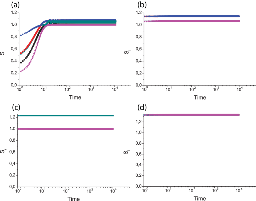
Figure 2: Simulations of the time evolution of the size of ($n=5$) agents for four different sets of initial conditions; all for $\sigma=0.01$. (a) CASE VI (2-1-1-1): the highest level with two agents (red and green) and the rest levels with one agent each one. Initial condition was chosen randomly in the range $[0,1]$. (b) CASE III (3-2): the highest level with three agents and the lowest level with two agents. (c) CASE II (4-1): the highest level with four agents and only one agent in the lowest level (d) CASE I (5): All agents in the same level. Initial conditions for (b), (c) and (d) were chosen very close to the corresponding FP in order to assure the convergence ($|s_{i}^{0}-s_{i}^{*}|<0.01$ with $s_{i}^{0}$ is the used initial condition and $s_{i}^{*}$ is the theoretical value at the fixed point).

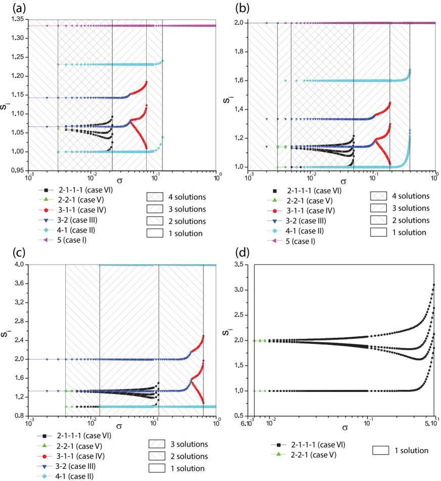
Figure 3: Agent sizes $s_{i}$ vs. $\sigma$ ($n=5$). Intervals in $\sigma$ with different numbers of overlapped solutions were found. (a) $K=-0.0625$ and five intervals: $0.001<\sigma\leq 0.003$ (2 solutions), $0.003<\sigma\leq 0.022$ (4 solutions), $0.022<\sigma\leq 0.077$ (3 solutions), $0.077<\sigma\leq 0.14$ (2 solutions) and $0.014<\sigma\leq 1$ (1 solution). (b) $K=-0.125$ and six intervals: $0.001<\sigma\leq 0.003$ (2 solutions), $0.003<\sigma\leq 0.005$ (3 solutions), $0.005<\sigma\leq 0.049$ (4 solutions), $0.049<\sigma\leq 0.186$ (3 solutions), $0.186<\sigma\leq 0.387$ (2 solutions) and $0.387<\sigma\leq 1$ (1 solution). (c) $K=-0.25$ and five intervals: $0.001<\sigma\leq 0.004$ (1 solution), $0.004<\sigma\leq 0.014$ (2 solutions), $0.014<\sigma\leq 0.12$ (3 solutions), $0.12<\sigma\leq 0.63$ (2 solutions) and $0.63<\sigma\leq 1$ (1 solution). (d) $K=-0.5$ and one interval with only one solution: $0.007<\sigma\leq 0.48$.

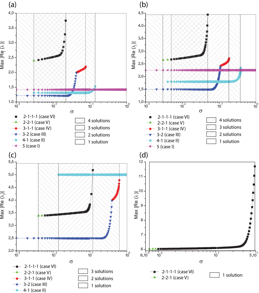
Figure 4: Maximum absolute eigenvalue real part of the Jacobian matrix vs. $\sigma$ value ($n=5$). (a) $K=-0.0625$ in the interval $0.003<\sigma\leq 0.022$ (4 solutions) the FP of type 2-1-1-1 (case VI) dominates over the rest. (b) $K=-0.125$ in the interval $0.005<\sigma\leq 0.049$ (4 solutions) the FP of type 2-1-1-1 (case VI) dominates over the rest. (c) $K=-0.25$ in the interval $0.014<\sigma\leq 0.12$ (3 solutions) the FP of type 4-1 (case II) dominates over the rest. (d) $K=-0.5$ in the interval $0.007<\sigma\leq 0.48$ there is only one solution.

Another meaningful and enlightening type of display shows the $\sigma$ dependence of stable FPs. In Figure 3, the agents sizes that correspond to each stable FP, as a function of parameter $\sigma$, are presented for a subset of representative values of the parameter $K$. To find these FPs, the NR method was used in order to find the roots of the corresponding non linear system of equations, using 100.000 random starting points, but finally keeping only the stable FP. To evaluate numerically the eigenvalues of the Jacobian matrix at different $\sigma$ values, a QR like algorithm was used. From such simulations, we confirm that there are several overlapping regions ($\sigma$ intervals) of stable configurations (see detailed explanations in the caption of Figure 3). In other words, for a given $\sigma$ value, clusters are possibly found with different asymptotic values $s_{i}$.

IV.3 Attractor strength

All eigenvalues have negative real part in the case of a stable fixed point. Moreover, the absolute value of the most negative eigenvalue real part is considered as determining the “force of the attractor” or the “speed of convergence” towards it strogatz2014nonlinear ; hilborn2000chaos . We have computed such an absolute maximum value of the real part of eigenvalues, at each stable fixed point versus $\sigma$. This is shown in Figure 4.

While the dynamics of the system is dominated by the FP with the highest absolute value of the real part of eigenvalue, nevertheless recall that the precise dynamics also depends on the initial conditions. For example, Figure 4 shows that the eigenvalue associated to the case (VI) (2-1-1-1) dominates that of the other fixed points, i.e. the probability of reaching this configuration is much higher than the other FP. Simulations have confirmed such a forecast.

The time evolution is non oscillatory in the case of 5 agents (see Figure 2), and it is also seen on Figures 5 and 6, in the case of 10 agents, where the transition time is very short not allowing to make a visually pleasant Poincare map.

V Simulations and results for $n=10$

Even though the case of $n\leq 5$ agents is fine enough to illustrate the main features of the model, and their consequences (they are also summarized in the conclusion section), one might wonder whether larger systems might present additional features. Thus, we present some additional simulations results for a system with only ten agents. In fact, we consider that this is quite a sufficient number in order to describe most of the economic fields, academically studied or not.

In order to span a large domain of cooperation possibilities, here $K=-0.25$ was used. The obtained behaviors are shown in Figures 5 and 6, for $\sigma=0.01$ and $\sigma=0.09$ respectively. These figures, illustrate that in this cooperative scenario, groups of agents are able to exceed their own size capacity limit determined by $\beta=1$ (without interaction, i.e. $\gamma\left(s_{i},s_{j}\right)=0$). It is noted that, in the example of Fig. 5, after a chaotic transition time interval, agents reach their steady state. On the other hand, for a larger $\sigma$, see Fig. 6, i.e. for a “long interaction size range”, the agents reach their steady state faster. In these examples, the strong cooperation of four agents allows them to reach a size equal to 4. There is another group consisting of three agents whose sizes are equal to 2. Then the third group is composed of two agents of size 1.33 for each one, and finally the smaller group consists of only one agent which size is equal 1. It is also emphasized that at this FP the steady state was always reached, indicating that its associated probability of occurrence, after a not too long time, is very close to 1.

Therefore, this mainly simulation study on a one-shot cooperation case ($K=-0.25$) confirms the findings for a smaller number of agents under the variation of the parameters and initial conditions, discussed in the other subsections.

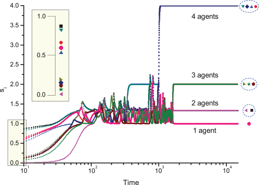
Figure 5: Simulation example of the time evolution of the model with $n=10$, $\sigma=0.01$ and $K=-0.25$: there are four final clusters, each containing 4, 3, 2 and 1 agents, respectively. It is highlighted that some agents with an initial small size are able to reach the highest level (see for example the agent denoted by a dark blue diamond). Conversely, some agents starting with a large size evolves to one of the lowest levels (see for example the agent denoted by a black square.)

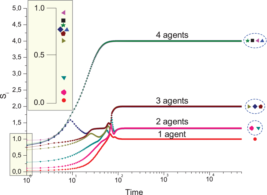
Figure 6: Simulation example of the time evolution of the model with $n=10$, $\sigma=0.09$ and $K=-0.25$: there are four final clusters, each containing 4, 3, 2 and 1 agents, respectively.

VI Conclusions and discussion

The study of complex systems a very active area of research. The mathematical tools developed in this field are so versatile that they allow applications to diverse kinds of problems in different research areas such as communication networks Kocarev ; IEEE2011 , biology Sitharama ; Bagni , socio-economy Huberman ; Yanhui , etc. We have considered a peer-to-peer interaction system, but allowing for cooperation between agents rather than competition.

In this work, we have found different behaviors. All lead to a structuration of the system with a remarkable group (cluster) hierarchy. Multiple stable solutions for a given $\sigma$ value can be found, but always one solution dominates. The largest group with the largest size markedly dominates in the system. Moreover, the dominating group occurs more quickly when the interaction encompasses a wider size range. It is interesting to note that the $\sigma$ value can be interpreted in a social or economical context as the way in which agents interact. For a small $\sigma$ value, the interaction is restricted to agents with very similar sizes and agents with different sizes do not interact with each other. On the other side, having a large $\sigma$ value allows agents with different sizes interact, which is close to the meaning of social equality. In other words, in the latter case, powerful (big) social groups are able to cooperate with weak (small) groups. In the case of an economical system, having a large $\sigma$ value may correspond to a free market situation in which all agents (big and small ones) are allowed to interact each other. On the other hand, having a small $\sigma$ value may correspond to the case of having government regulations that constrain the agents to interact with only agents of similar sizes.

Summarizing, sometimes a solution, e.g. case (VII) in Sect. IV.2 is never stable, regardless of $\sigma$, $K$ and $n$ values, while cases are always stable for $K>\frac{-1}{n-1}$, e.g. case (I). According to $\sigma$ ranges, the spread of cooperation, there are stable steady states, but sometimes not. Thus, it is possible to have more than one stable configuration, … two, three or even four, in the 5-agent case, depending on the $\sigma$ value. Moreover, the ranges of $\sigma$ where the steady state solution is unique can be also observed, (see Table 1). Stressing the $K$ value order of magnitude, like $K=-1$, case no stable solution is found, regardless of the $\sigma$ value

After making a large number ($10^{4}$) of numerical simulations for uniformly distributed random initial conditions, we have always obtained the solution corresponding to the eigenvalue with highest absolute value of the real part. This suggests that the probability to obtain other solutions is almost vanishing. In contrast, for non-uniformly distributed initial conditions and in particular those close to other relevant fixed points, possible solutions emerge. In so doing, we can claim that there is much coherence in the model.

From a “practical” point of view, our main finding has been to show the power of cooperation in order to increase “size”. When agents cooperate, they are able to triply or even quadruply increase their size, in some sense their market share. This should be contrasted with previous studies in which the competitive scenario leads to the winner takes all: agents are clustered at sizes lower than 1, i.e. their theoretical capacity when behaving independently of each other Huberman ; Huberman2 ; Caram . Cooperation, instead, allows for the group of cooperative agents to configure a cluster with a characteristic level higher than the individual capacity, obtained without interactions, which is defined by the $\beta=1$ value.

The model describes approximately what is happening in society, at least in common sense expectations. Consider a few examples (i) ”cooperation rather than competition between Coca-Cola and Pepsi-Cola in order to share the market and avoid many intruders; (ii) cooperation between a few co-authors in order to improve their number of publications, citations, whence h-index; (iii) in sport, cooperation (within theoretical competition) in order to win a race or a game; (iv) cooperation in the car industry in order to be the first to propose an electric car (Daimler AG, parent of Mercedes-Benz cooperate with Tesla Motors; Renault Nissan Alliance has made agreements to promote emission-free mobility in France, Israel, Portugal, Denmark); (v) let us briefly mention competition AND cooperation between political parties in order to form a coalition government (when the cooperating weakest ones can overcome the top party, though a case indeed not found in our model)

It is highlighted that we have considered here only symmetric interactions allowing us to unveil the main advantages of cooperation. It is worth mentioning that in real cooperative socio-economical systems sometimes not all agents cooperate in the same way. This important characteristic of real systems could be incorporated in the model through an asymmetric interaction kernel in a future work, for example, by considering $K_{ij}$ and $K_{ji}$ or $\sigma_{ij}$ and $\sigma_{ji}$ to be different. We think that tue current model, rather than representing a real world system faithfully, it help us to understand the behavior of agents in an ideal cooperative scenario. In real world, there are mixed types of interactions including cooperation and competition. For example, in real world, it is expected that some groups of agents cooperate with each other within the group and compete with agents outside the group. We plan to study these more realistic multiagent systems in the future by simulations.

It is outside the aim of this paper to discuss whether the economic environment determines whether the fair types or the selfish types dominate equilibrium behavior, nor whether cooperation or competition has to be favorized fehr1999theory . It should be surely interesting in further work to adapt the model to very specific cases, e.g., to research, sport or other socio-economic activities. Recall that the time scale can be adapted. Moreover spatial distribution Damero , transport costs, and similar economic considerations could introduce new parameters.

Acknowledgements This paper is part of MA scientific activities in COST Action IS1104, “The EU in the new complex geography of economic systems: models, tools and policy evaluation”, in COST Action TD1210 ‘Analyzing the dynamics of information and knowledge landscapes’, and in COST Action TD1306 “New Frontiers of Peer Review”.

Table 1: Fixed points and their $\sigma$ stability interval for the $n=5$ agent case, for various $K<0$.

Cases	N∘ Levels	N∘ Agents	$K=-0.0625$	$K=-0.125$	$K=-0.25$	$K=-0.5$	$K=-1$
		by	4 overlapping	4 overlapping	3 overlapping	only one	non stable
		level	stable configurations	stable configurations	stable configurations	stable configuration	configuration
I	1	5	always stable	always stable	never stable	never stable	never stable
II	2	4-1	$0.003\leq\sigma\leq 0.140$	$0.004\leq\sigma\leq 0.387$	$0.014\leq\sigma$	never stable	never stable
III	2	3-2	$0.001\leq\sigma\leq 0.043$	$0.001\leq\sigma\leq 0.109$	$0.001\leq\sigma\leq 0.4$	never stable	never stable
IV	3	3-1-1	$0.044\leq\sigma\leq 0.077$	$0.110\leq\sigma\leq 0.186$	$0.410\leq\sigma\leq 0.630$	never stable	never stable
V	3	2-2-1	$0.003=\sigma$	$0.003\leq\sigma\leq 0.004$	$0.004\leq\sigma\leq 0.005$	$0.007\leq\sigma\leq 0.009$	never stable
VI	4	2-1-1-1	$0.004\leq\sigma\leq 0.022$	$0.005\leq\sigma\leq 0.049$	$0.006\leq\sigma\leq 0.12$	$0.010\leq\sigma\leq 0.480$	never stable
VII	5	1-1-1-1-1	never stable	never stable	never stable	never stable	never stable

References

- (1) C. Darwin, On the Origin of Species by Means of Natural Selection, or the Preservation of Favoured Races in the Struggle for Life, 5th ed. (London: John Murray, 1869, retrieved Feb. 22, 2009).
- (2) M. Dorigo and T. St utzle, Ant Colony Optimization (Cambridge, MA:MIT, 2004).
- (3) Y. Hayashi, M. Yuki, K. Sugawara, T. Kikuchi, and K. Tsuji, Artificial Life and Robotics 13, 120 (2008).
- (4) E. Fehr and K. M. Schmidt, The Quarterly Journal of Economics 114, 817 (1999).
- (5) G. Hamel, Y. L. Doz, and C. K. Prahalad, Harvard Business Review 67, 133 (1989).
- (6) F. Schweitzer and L. Behera, Advances in Complex Systems 15, 1250059 (2012).
- (7) X. Luo, R. J. Slotegraaf, and X. Pan, Journal of Marketing 70, 67 (2006).
- (8) C. Hauert, Advances in Complex Systems 9, 315 (2006).
- (9) F. Schweitzer and L. Behera, Advances in Complex Systems 15, 1250059 (2012).
- (10) A. Barreira Da Silva Rocha and A. Laruelle, Advances in Complex Systems 16, 1350036 (2013).
- (11) N. Boccara, Modeling Complex Systems (Kluwer Academic Publishers, 2004).
- (12) Y. Bar-Yam, Dynamics of complex systems (Addison-Wesley, 1997).
- (13) H. N. Knyazeva and S. P. Kurdyumov, Evolution and Self-organization Laws of Complex Systems (Nauka Publisher, Moscow, 1994) p. p 236.
- (14) M. E. Porter, Economic Development Quarterly 14, 15 (2000).
- (15) A. Lotka, Elements of Physical Biology (Williams & Wilkins Company, 1925).
- (16) V. Volterra, Mem. R. Accad. Naz. dei Lincei VI, 2 (1926).
- (17) S. M. Maurer and B. A. Huberman, Journal of Economic Dynamics and Control 27, 2195 (2003).
- (18) L. A. Adamic and B. A. Huberman, Quart. J. Electron. Comm. 1, 5 (2000).
- (19) L. Yanhui and Z. Siming, Appl. Math. Modelling 31, 912 (2007).
- (20) L. Caram, C. Caiafa, A. Proto, and M. Ausloos, Physica A: Statistical Mechanics and its Applications 389, 2628 (2010).
- (21) P.-F. Verhulst, Nouv. mém. de l’Académie Royale des Sci. et Belles-Lettres de Bruxelles 18, 1 (1845).
- (22) P.-F. Verhulst, Mém. de l’Académie Royale des Sci., des Lettres et des Beaux-Arts de Belgique 20, 1 (1847).
- (23) D. S. Broomhead and D. Lowe, Complex Systems 2, 321 (1988).
- (24) S. Strogatz, Nonlinear Dynamics and Chaos: With Applications to Physics, Biology, Chem- istry, and Engineering, Studies in Nonlinearity (Westview Press, 2014) Chap. 5 and 6.
- (25) W. H. Press, S. A. Teukolsky, W. T. Vetterling, and B. P. Flannery, Numerical Recipes in FORTRAN; The Art of Scientific Computing, 2nd ed. (Cambridge University Press, New York, NY, USA, 1993).
- (26) R. Hilborn, Chaos and Nonlinear Dynamics: An Introduction for Scientists and Engineers (Oxford University Press, 2000) Chap. 4.
- (27) L. Kocarev and G. Vattay, Complex Dynamics in Communication Networks (Springer Verlag, 2005).
- (28) C. Michalakelis, T. Sphicopoulos, and D. Varoutas, IEEE Transactions on Systems, Man, and Cybernetics 41, 200 (2011).
- (29) S. Sitharama Iyengar, Computer Modeling and Simulations of Complex Biological Systems (2nd edn. CRC, 1997).
- (30) R. Bagni, R. Berchi, and P. Cariello, Journal of Artificial Societies and Social Simulation 5 (2002), http://jasss.soc.surrey.ac.uk/5/3/5.html.
- (31) C. Caiafa and A. Proto, International Journal of Modern Physics C 17, 385 (2006).