Stochastic Analysis Of An Incoherent Feedforward Genetic Motif

Abstract

Gene products (RNAs, proteins) often occur at low molecular counts inside individual cells, and hence are subject to considerable random fluctuations (noise) in copy number over time. Not surprisingly, cells encode diverse regulatory mechanisms to buffer noise. One such mechanism is the incoherent feedforward circuit. We analyze a simplistic version of this circuit, where an upstream regulator $X$ affects both the production and degradation of a protein $Y$. Thus, any random increase in $X$’s copy numbers would increase both production and degradation, keeping $Y$ levels unchanged. To study its stochastic dynamics, we formulate this network into a mathematical model using the Chemical Master Equation formulation. We prove that if the functional dependence of $Y$’s production and degradation on $X$ is similar, then the steady-distribution of $Y$’s copy numbers is independent of $X$. To investigate how fluctuations in $Y$ propagate downstream, a protein $Z$ whose production rate only depend on $Y$ is introduced. Intriguingly, results show that the extent of noise in $Z$ increases with noise in $X$, in spite of the fact that the magnitude of noise in $Y$ is invariant of $X$. Such counter intuitive results arise because $X$ enhances the time-scale of fluctuations in $Y$, which amplifies fluctuations in downstream processes. In summary, while feedforward systems can buffer a protein from noise in its upstream regulators, noise can propagate downstream due to changes in the time-scale of fluctuations.

I Introduction

The inherent probabilistic nature of biochemical reactions and low copy numbers of molecules involved, results in significant random fluctuations (noise) in mRNA/protein levels inside individual cells [1, 2, 3, 4, 5, 6, 7, 8, 9]. These fluctuations are an unavoidable aspect of life at the single-cell level. Noise can be problematic for essential proteins whose levels have to be tightly maintained within certain bounds [10, 11, 12], and various diseased states have been attributed to elevated noise in the expression of certain genes [13, 14, 15, 16]. Interestingly, this inherent variation in gene product levels is sometimes exploited for driving genetically identical cells to different fates [17, 18, 19, 20, 21, 22], as is the case for many stem cells [23, 24, 25] and pathogenic human viruses [26, 27, 28, 29].

Given that stochasticity in protein levels can have significant effects on biological function and phenotype, cells actively use different regulatory mechanisms to minimize noise. Much prior experimental/computational work on noise buffering has primarily focused on negative feedback systems, where a protein controls its own transcription/translation/degradation [30, 31, 32, 33, 34, 35, 36, 37, 38, 39, 40, 41, 42, 43]. Here we focus on feedforward systems, where a downstream regulator affects the expression of a protein using two different paths. More specifically, we study the incoherent feedforward loop, where the paths have antagonistic affects [44, 45, 46]. Such incoherent feedforward regulation has been shown to be an important motif in gene regulatory networks [45, 46, 47].

The schematic of the overall network is illustrated in Fig. 1 and consists of three species: an upstream regulator $X$, protein $Y$, and a downstream product $Z$ that is activated by $Y$. In the model under consideration, $X$ enhances both the production and degradation of $Y$, creating an incoherent feedforward circuit. In the stochastic formulation of this network, each specie is assumed to be produced in random bursts [48, 49, 50]. More specifically, bursts for the creation of $X$ arrive at exponentially distributed time intervals with rate $k_{X}$. Each burst results in the production of $n_{X}$ molecules of $X$, where $n_{X}$ is geometrically distributed random variable. $X$ is assumed to degrade at a constant rate $\gamma_{X}$. Finally, we denote by $x(t)$, the stochastic process representing the population count of $X$ in a single cell. The same nomenclature applies for $Y$ and $Z$.

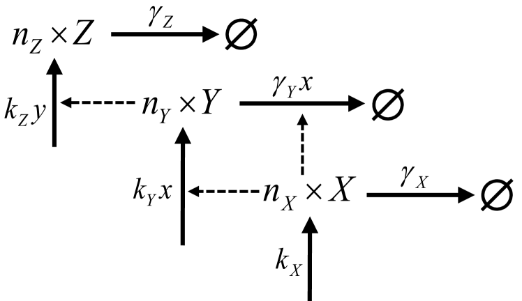
Figure 1: Schematic figure of the model under consideration. $X$ affects both the production and degradation of Y, which itself activates production of downstream product $Z$. The creation and degradation rates of molecules $X$, $Y$ and $Z$ are denotes $k_{X}$, $\gamma_{X}$, $k_{Y}$, $\gamma_{Y}$ and $k_{Z}$, $\gamma_{Z}$. Each creation event generates a burst, of size $n_{\bf j}$, characterized by a geometrical distribution $g(n_{\bf j}|\bar{b}_{\bf j})$ with mean ${\bar{b}_{\bf j}}$ (for ${\bf j}=X,Y,Z$).

 

Our goal is to use this model to study how random fluctuations in the levels of $X$ propagate to $Y$ and $Z$. Results show that if the functional dependence of $Y$’s production and degradation on $X$ is similar, then the steady-distribution of $Y$’s copy numbers is independent of $X$. Thus, the feedforward regulation completely buffers $Y$ from random fluctuations in the upstream regulator. Interestingly, fluctuations in $X$ enhance the time-scale of fluctuation in $Y$, as quantified by the steady-state autocorrelation function. This implies that fluctuations in $X$ make fluctuations in $Y$ more permanent while keeping their magnitude unchanged, leading to an amplified noise in the downstream product $Z$.

The paper is organized as follows. In section II, we present a stochastic model for the expression of protein $Y$, with constant production and degradation rates. In section III, we consider the effect of the upstream regulator $X$ on $Y$’s production process. In section IV, $X$ is assumed to affect both production and degradation processes of $Y$, creating a feedforward system. The autocorrelation function of $Y$ is derived in section V. Finally, in section VI we quantify the noise in the downstream product $Z$.

II Single protein model with constant rates

We start by considering the model (summarised by table I) describing the dynamics of the number of molecules $Y$, with constant production and degradation rates.

Event	Reset	Transition rates
burst of $n_{Y}$ $Y$ molecules	$y\rightarrow y+n_{Y}$	$k_{Y}g(n_{Y}|{\bar{b}_{Y}})$
degradation	$y\rightarrow y-1$	$y\gamma_{Y}$

TABLE I: Transitions and associated rates for the single protein model with constant rates

We write $k_{Y}\delta t$ the probability of a burst occurring in a time $\delta t$. Each burst is drawn from a geometric distribution:

$$g(n_{Y}|{\bar{b}_{Y}})={(\bar{b}_{Y})^{n_{Y}}}/{(1+{\bar{b}_{Y}})^{{n_{Y}}+1}},$$ (1)

with mean ${\bar{b}_{Y}}=\sum_{{n_{Y}}}{n_{Y}}g({n_{Y}}|{\bar{b}_{Y}})$. In a time interval $\delta t$, the probability of occurrence of a burst of size ${n_{Y}}$ is therefore given by $k_{Y}g({n_{Y}}|{\bar{b}_{Y}})\delta t$. In addition, we denote by $\gamma_{Y}$ the degradation rate so that the probability of the transition, from a state with $y$ molecules to a state with $y-1$ molecules, in a time $\delta t$, is given by $y\gamma_{Y}\delta t$. It is well known that the probability $P_{y}(t)$ to measure $y$ molecules at time $t$, obeys the master equation [51, 52, 53]

$$\frac{dP_{y}(t)}{dt} = k_{Y}\left[\sum_{n_{Y}=0}^{y}g(n_{Y}|{\bar{b}_{Y}})P_{y-n_{Y}}(t)-P_{y}(t)\right]$$ (2)

$$+ \gamma_{Y}\Big{[}(y+1)P_{y+1}(t)-yP_{y}(t)\Big{]}.$$

The latter equation gives a full description of the stochastic process under consideration. It is, however, common practice to express such problem in term of the generating function defined as $G(r,t)=\sum_{y}P_{y}(t)r^{y}$. Derived from (2) the equation for the generating function is:

$$\frac{dG}{dt}=k_{Y}(\tilde{g}-1)G-\gamma_{Y}(r-1)\partial_{r}G,$$ (3)

where $\tilde{g}$ is the generating function of the distribution $g(n_{Y}|{\bar{b}_{Y}})$ and given by

$$\tilde{g}(r|{\bar{b}_{Y}})=\sum_{n_{Y}=0}^{\infty}r^{n_{Y}}g(n_{Y}|{\bar{b}_{Y}})=\frac{1}{1+{\bar{b}_{Y}}(1-r)}.$$ (4)

Equation (3) offers an easy path towards the solution of our problem. In particular, in the limit $t\rightarrow\infty$, we find

$$G(r)=\frac{1}{\left[1+{\bar{b}_{Y}}(1-r)\right]^{k_{Y}/\gamma_{Y}}}.$$ (5)

At this stage the inverse transfomation,

$$P(y=n)=\lim_{r\rightarrow 0}\frac{1}{n!}\frac{d^{n}G(r)}{dr^{n}},$$ (6)

can be used to access the stationary probability distribution which, in this case, is a negative binomial distribution:

$$P(y=n) = \frac{1}{n!}\left(\frac{\bar{b}_{Y}}{1+\bar{b}_{Y}}\right)^{n}\left(\frac{1}{1+\bar{b}_{Y}}\right)^{\frac{k_{Y}}{\gamma_{Y}}}$$

$$\times \prod_{j=0}^{n-1}\left(j+\frac{k_{Y}}{\gamma_{Y}}\right).$$

One can directly access first and second order moments using

$$\langle y\rangle=\left.\frac{dG(r)}{dr}\right|_{r\rightarrow 1},\text{ and }\langle y(y-1)\rangle=\left.\frac{d^{2}G(r)}{dr^{2}}\right|_{r\rightarrow 1},$$ (8)

which leads to the mean number

$$\langle y\rangle=\frac{k_{Y}{\bar{b}_{Y}}}{\gamma_{Y}}.$$ (9)

We will use the coefficient of variation $CV_{Y}^{2}$ as metric for quantifying noise. It is defined by

$$CV_{Y}^{2}=\frac{\langle y^{2}\rangle-\langle y\rangle^{2}}{\langle y\rangle^{2}},$$

and given by

$$CV_{Y}^{2}=\frac{1+{\bar{b}_{Y}}}{\langle y\rangle}.$$ (10)

Unless stated otherwise $\langle y\rangle$ denotes the average in the stationary state. We will be explicitly using $\langle y(t)\rangle$ to refer to the average number at intermediate times. At this point, the reader may want to consider a similar problem for a non-bursty production (each production event generating exactly one molecule). To proceed, the reader may simply replace $k_{Y}$ by $k_{Y}/{\bar{b}_{Y}}$ and take the limit ${\bar{b}_{Y}}\rightarrow 0$. This transformation comes from the need to reduce the term $g(r|{\bar{b}_{Y}})-1$, in (3), into $y-1$. Under this transformation we recover the Poisson distribution

$$G(r)\rightarrow\exp\left[{\frac{k_{Y}}{\gamma_{Y}}(r-1)}\right],$$ (11)

characterized by the mean and coefficient of variation

$$\langle y\rangle\rightarrow\frac{k_{Y}}{\gamma_{Y}},\text{ and }CV_{Y}^{2}\rightarrow\frac{1}{\langle y\rangle}.$$ (12)

III Regulation of the creation process

We now focus our attention on a variation of the model presented in section II for which molecule production is regulated by an upstream process. Here the bursty creation process of $Y$ is governed by another dynamical process. A new random variable $x$ is introduced describing the number of molecules of type $X$. The extra dynamical variable $x$ now appears explicitly in the bursty production rate which becomes $xk_{Y}$. We choose to consider $X$ as governed by a bursty creation process with single degradation. We write $k_{X}$ and $\gamma_{X}$ the creation and degradation rates. Each burst of $X$ is distributed by $g({n_{X}}|{\bar{b}_{X}})$ where ${\bar{b}_{X}}$ denotes the mean burst size. All transition rates are summarized in table II. We choose not to write the full master equation associated to the evolution of the distribution $P_{x,y}(t)$. We however give the key steps leading to the moment equations. To proceed the reader may derive a generalized moment equation [54, 55]

$$\frac{d\langle x^{\sigma}y^{\eta}\rangle}{dt} = k_{X}\langle\left[(x+n_{X})^{\sigma}-x^{\sigma}\right]y^{\eta}\rangle$$

$$+ \gamma_{X}\langle x\left[(x-1)^{\sigma}-x^{\sigma}\right]y^{\eta}\rangle$$

$$+ k_{Y}\langle x^{\sigma+1}\left[(y+n_{Y})^{\eta}-y^{\eta}\right]\rangle$$

$$+ \gamma_{Y}\langle x^{\sigma}\left[(y-1)^{\eta}-y^{\eta}\right]y\rangle,$$

for $\sigma$ and $\eta$ integers. The latter equation leads to the first order moments

$$\frac{d\langle x(t)\rangle}{dt} = k_{X}{\bar{b}_{X}}-\gamma_{X}\langle x(t)\rangle,$$ (14)

$$\frac{d\langle y(t)\rangle}{dt} = k_{Y}{\bar{b}_{Y}}\langle x(t)\rangle-\gamma_{Y}\langle y(t)\rangle,$$ (15)

as well as second order moments

$$\frac{d\langle x^{2}(t)\rangle}{dt} = k_{X}{\bar{b}_{X}}[2\langle x(t)\rangle+2{\bar{b}_{X}}+1]$$

$$+ \gamma_{X}[\langle x(t)\rangle-2\langle x^{2}(t)\rangle],$$

$$\frac{d\langle y^{2}(t)\rangle}{dt} = k_{Y}{\bar{b}_{Y}}\left[2\langle xy(t)\rangle+(2{\bar{b}_{Y}}+1)\langle x(t)\rangle\right]$$

$$+ \gamma_{Y}\left[\langle y(t)\rangle-2\langle y^{2}(t)\rangle\right],$$

$$\frac{d\langle xy(t)\rangle}{dt} = k_{X}{\bar{b}_{X}}\langle y(t)\rangle+k_{Y}{\bar{b}_{Y}}\langle x^{2}(t)\rangle$$

$$- (\gamma_{X}+\gamma_{Y})\langle xy(t)\rangle.$$

Event	Reset	Transition rates
burst of $n_{X}$ $X$ molecules	$x\rightarrow x+n_{X}$	$k_{X}g(n_{X}|{\bar{b}_{X}})$
$X$-degradation	$x\rightarrow x-1$	x$\gamma_{X}$
burst of $n_{Y}$ $Y$ molecules	$y\rightarrow y+n_{Y}$	${x}k_{Y}g(n_{Y}|{\bar{b}_{Y}})$
$Y$-degradation	$y\rightarrow y-1$	$y\gamma_{Y}$

TABLE II: Transitions and associated rates for a model with regulated creation process.

The previous set of equations being closed one can easily show that the stationary state is characterized by the mean numbers

$$\langle x\rangle=\frac{k_{X}{\bar{b}_{X}}}{\gamma_{X}}\text{ and }\langle y\rangle=\frac{k_{Y}{\bar{b}_{Y}}}{\gamma_{Y}}\langle x\rangle,$$ (19)

with the following coefficients of variation

$$CV_{X}^{2} = \frac{1+{\bar{b}_{X}}}{\langle x\rangle},$$ (20)

$$CV_{Y}^{2} = \frac{1+{\bar{b}_{Y}}}{\langle y\rangle}+\frac{\gamma_{Y}}{\gamma_{X}+\gamma_{Y}}\frac{1+{\bar{b}_{X}}}{\langle x\rangle}.$$ (21)

Note that $CV_{Y}^{2}$ is the sum of two contributions. The first term represents the noise in the single protein model with constant rates. The second term is the noise contribution from upstream regulation. We note that both $\langle y\rangle$ and $CV_{Y}^{2}$ are dependent on the upstream dynamics (dependence in $k_{X}$, $b_{X}$ and $\gamma_{X}$). The dependence in the $X$ dynamics will however vanished in the next section when considering regulated production and degradation.

IV Incoherent feedforward circuit

To move one step forward we choose to consider a model where both the production and degradation are affected by the dynamics of $X$, therefore defining a feedforward motif. We define $xk_{Y}$ and $x\gamma_{Y}$ as the new creation and degradation rates. All transition rates are summarized in table III and illustrated on Fig. 1.

Event	Reset	Transition rates
burst of $n_{X}$ $X$ molecules	$x\rightarrow x+n_{X}$	$k_{X}g(n_{X}|{\bar{b}_{X}})$
$X$-degradation	$x\rightarrow x-1$	$x\gamma_{X}$
burst of $n_{Y}$ $Y$ molecules	$y\rightarrow y+n_{Y}$	$xk_{Y}g(n_{Y}|{\bar{b}_{Y}})$
$Y$-degradation	$y\rightarrow y-1$	$xy\gamma_{Y}$

TABLE III: Transitions and associated rates for an incoherent feedforward circuit.

The probability $P_{x,y}(t)$ is governed by the master equation

$$\frac{dP_{x,y}(t)}{dt} = k_{X}\left[\sum_{n_{X}=0}^{x}g(n_{X}|{\bar{b}_{X}})P_{x-n,y}-P_{x,y}\right]$$

$$+ \gamma_{X}\left[(x+1)P_{x+1,y}-xP_{x,y}\right]$$

$$+ xk_{Y}\left[\sum_{n_{Y}=0}^{y}g(n_{Y}|{\bar{b}_{Y}})P_{x,y-n}-P_{x,y}\right]$$

$$+ x\gamma_{Y}\Big{[}(y+1)P_{x,y+1}-yP_{x,y}\Big{]}.$$

It is then important to note that, in the stationary state, writing $P_{x,y}=Q_{x}R_{y}$ allows to split (IV) in two:

$$k_{X}\sum_{n_{X}=0}^{x}g(n_{X}|{\bar{b}_{X}})Q_{x-n}+\gamma_{X}(x+1)Q_{x+1}$$ (23)

$$=(k_{X}+\gamma_{X}x)Q_{x},$$

$$k_{Y}\sum_{n_{Y}=0}^{y}g(n_{Y}|{\bar{b}_{Y}})R_{y-n}+\gamma_{Y}(y+1)R_{y+1}$$ (24)

$$=(k_{Y}+\gamma_{Y}y)R_{y}.$$

Note that (23) and (24) have exactly the same form but more importantly are independent. It follows that the $x$ and $y$ variables are uncorrelated. The average $\langle y\rangle$ and all other moments are independents of $k_{X}$, $\gamma_{X}$ and ${\bar{b}_{X}}$. It is important to mention that an identical derivation can be repeated in a much more general scenario: First by generalizing this result for any production and degradation rates of the form $k_{Y}(x)=k_{Y}f(x)$ and $\gamma_{Y}(x)=\gamma_{Y}f(x)$ (for an arbitrary function $f$). Secondly by relaxing constrains on the dynamics of $X$ and writing $W^{x}_{x^{\prime}}$ as the transition rate associated to $x\rightarrow x^{\prime}$ (with the restriction that $W^{x}_{x^{\prime}}$ is independent of $y$). Once again, a similar derivation will show that the mean number of $Y$ molecules and all moments are independent of the upstream process associated to $X$.

As a consequence, when looking at the stationary distribution of $x$ only, one would not be able to distinguish the model with feedfoward motif (regulated creation and degradation) from the single protein model (with no input noise at all). In a sense, the $x$ variable and its dynamics are “hidden” in the stationary state. However, a signature of this “hidden variable” may be observed someplace else. Indication that the process is or not governed by a “hidden” dynamics could be found in dynamical data. Since the equality $P_{x,y}=Q_{x}R_{y}$ holds true in the stationary state only, the analysis of transient regime should give evidences of the upstream process. For example, one could study quantities such as relaxation time and autocorrelations, which would, in principle, testify of the existence of $X$. Interestingly, another indication of the existence of an upstream noise is to be found in downstream production. In the next sections we look for signature of an upstream regulator in both autocorrelation function and downstream processes.

V Effect of Feedforward regulation on autocorrelation time

In the following we present an analytical study of the autocorrelation function. We first start with a presentation of the method used, considering the single protein model with constant production rates (summarized in table I). The $Y$ autocorrelation function for the model presented in table III and illustrated in Fig. 1 is however unknown and its calculation appears extremely challenging. We therefore consider a feeforward model regulated by a binary process as illustrated in Fig. 3 and summarized in table IV. In the stationary state, it is common to study the normalized autocorrelation function defined by

$$R(t):=\lim_{s\rightarrow\infty}\frac{\langle y(t+s)y(s)\rangle-\langle y\rangle^{2}}{\langle y^{2}\rangle-\langle y\rangle^{2}}.$$ (25)

To progress further we use the relation

$$\langle y(t+s)y(s)\rangle=\langle y(s)\langle y(t+s)|y(s)\rangle\rangle,$$ (26)

where $\langle y(t+s)|y(s)\rangle$ is the expected number of molecules at time $t+s$ given $y(s)$ [56, 57]. Using theorem 1 of [58], we see that the time derivative of the expected value of any function $\varphi(y)$ is given by

$$\frac{d\langle\varphi(y)\rangle}{dt}=\left\langle\sum_{Events}\Delta\varphi(y)\times f(y)\right\rangle,$$ (27)

where $\Delta\varphi$ is change in function $\varphi$ when an event occurs and $f(y)$ denotes the transition rates of events and shows how often an event happens.

V-A Single protein model with constant rates

Considering the model with single protein, equation (27) for $\varphi(y)=y$ gives

$$\frac{d\langle y(t)\rangle}{dt}=k_{Y}{\bar{b}_{Y}}-\gamma_{Y}\langle y(t)\rangle,$$ (28)

and leads to the stationary values given in (9). It follows that the mean count at time $t$ knowing $y(s)$ is given by

$$\langle y(t+s)|y(s)\rangle={\langle y\rangle}+\left[y(s)-{\langle y\rangle}\right]e^{-\gamma_{Y}t}.$$ (29)

Using (26) together with (29) leads to

$$\langle y(t+s)y(s)\rangle={\langle y\rangle}^{2}+\left[{\langle y^{2}\rangle}-{\langle y\rangle}^{2}\right]e^{-\gamma_{Y}t}.$$ (30)

By substituting (30) in (25) we obtain the autocorrelation function which appears to be completely determined by the degradation rate:

$$R(t)=\exp\left({-\gamma_{Y}t}\right).$$ (31)

Event	Reset	Transition rates
Switch activation	$x\rightarrow x+1$	$(1-x)\alpha$
Switch deactivation	$x\rightarrow x-1$	$x\beta$
burst of $n_{Y}$ $Y$ molecules	$y\rightarrow y+n_{Y}$	$xk_{Y}g(n_{Y}|{\bar{b}_{Y}})$
$Y$-degradation	$y\rightarrow y-1$	$xy\gamma_{Y}$

TABLE IV: Transitions and associated rates for a model regulated by a biological switch.

V-B A model regulated by a biological switch

We now evaluate the autocorrelation function for a model where the upstream regulator is restricted to the values $x=0$ and $x=1$ (see Fig. 2). This model, should be regarded as a first step towards a more complex model. In fact, H. Pendar and collaborators [59] have shown that any birth-death process can be split into an infinite number of identical reduced models, each build as biological switches. In this picture, biological switches appears as the basic construction brick for more sophisticated models. We write $\alpha$ and $\beta$ the transition rates associated $x:0\rightarrow 1$ and $x:1\rightarrow 0$ and summarized in table IV. This chemical switch regulates both bursty production and degradation of molecules of type $Y$. For this particular model, we derive the moment equations

$$\frac{d\langle x(t)\rangle}{dt} = \alpha-(\alpha+\beta)\langle x(t)\rangle,$$ (32)

$$\frac{d\langle y(t)\rangle}{dt} = k_{Y}{\bar{b}_{Y}}\langle x(t)\rangle-\gamma_{Y}\langle xy(t)\rangle,$$ (33)

$$\frac{d\langle xy(t)\rangle}{dt} = \alpha\langle y(t)\rangle-(\alpha+\beta)\langle xy(t)\rangle$$

$$+ k_{Y}{\bar{b}_{Y}}\langle x(t)\rangle-\gamma_{Y}\langle xy(t)\rangle.$$

Solving equations (32)-(V-B) for initial conditions $x(s)$, $y(s)$ and $xy(s)$ result in

$$\langle y(t+s)|x(s),y(s),xy(s)\rangle={\langle y\rangle}$$

$$+ {\exp}\left[{-(\alpha+\beta+\gamma_{Y})\frac{t}{2}}\right]$$

$$\times \frac{\sinh\left(\frac{t}{2}\sqrt{(\alpha+\beta+\gamma_{Y})^{2}-4\alpha\gamma_{Y}}\right)}{\sqrt{(\alpha+\beta+\gamma_{Y})^{2}-4\alpha\gamma_{Y}}}$$

$$\times ((\alpha+\beta+\gamma_{Y})\left[y(s)-{\langle y\rangle}\right]+2\bar{b}_{Y}\left[x(s)-{\langle x\rangle}\right]$$

$$- 2\gamma_{Y}\left[xy(s)-{\langle xy\rangle}\right])$$

$$+ {\exp}\left[{-(\alpha+\beta+\gamma_{y})\frac{t}{2}}\right]$$

$$\times \cosh\left(\frac{1}{2}t\sqrt{(\alpha+\beta+\gamma_{Y})^{2}-4\alpha\gamma_{Y}}\right)\left[y(s)-{\langle y\rangle}\right]$$

Together with (26) the previous result leads to

$$\langle y(t+s)y(s)\rangle={\langle y\rangle}^{2}$$

$$+ (\alpha+\beta+\gamma_{Y}){\exp}\left[{-(\alpha+\beta+\gamma_{Y})\frac{t}{2}}\right]$$

$$\times \frac{\sinh\left(\frac{t}{2}\sqrt{(\alpha+\beta+\gamma_{Y})^{2}-4\alpha\gamma_{Y}}\right)}{\sqrt{(\alpha+\beta+\gamma_{Y})^{2}-4\alpha\gamma_{Y}}}\left({\langle y^{2}\rangle}-{\langle y\rangle}^{2}\right)$$

$$+ \exp\left[{-(\alpha+\beta+\gamma_{y})\frac{t}{2}}\right]$$

$$\times \cosh\left(\frac{t}{2}\sqrt{(\alpha+\beta+\gamma_{Y})^{2}-4\alpha\gamma_{Y}}\right)\left({\langle y^{2}\rangle}-{\langle y\rangle}^{2}\right)$$

$$+ {\exp}\left[{-(\alpha+\beta+\gamma_{Y})\frac{t}{2}}\right].$$

$$\times \frac{\sinh\left(\frac{t}{2}\sqrt{(\alpha+\beta+\gamma_{Y})^{2}-4\alpha\gamma_{Y}}\right)}{\sqrt{(\alpha+\beta+\gamma_{Y})^{2}-4\alpha\gamma_{Y}}}$$

$$\times \left(2\bar{b}_{Y}\left({\langle xy\rangle}-{\langle x\rangle}{\langle y\rangle}\right)-2\gamma_{Y}\left({\langle xy^{2}\rangle}-{\langle xy\rangle}{\langle y\rangle}\right)\right)$$

In order to find $\langle y(t+s)y(s)\rangle$ we need to find expression of $\langle xy^{2}\rangle$. Thus we add dynamics of $\langle y^{2}\rangle$ and $\langle xy^{2}\rangle$ to the set of moments dynamics presented in (32)-(V-B). Note that $x(t)$ is a Bernoulli random variable thus we have the following relations

$$\langle x^{q}\rangle=\langle x\rangle,\ \ \ \langle x^{q}y^{b}\rangle=\langle xy^{b}\rangle,\ \ \ q\in\{1,2,\ldots\}.$$ (37)

Using these characteristics, the moments dynamics of $\langle y^{2}\rangle$ and $\langle xy^{2}\rangle$ can be written as

$$\frac{d\langle y^{2}(t)\rangle}{dt} = k_{Y}\bar{b_{Y}}(2\bar{b}_{Y}+1)\langle x(t)\rangle+2k_{Y}{\bar{b}_{Y}}\langle xy(t)\rangle$$ (38)

$$+ \gamma_{Y}\langle xy(t)\rangle-2\gamma_{Y}\langle xy^{2}(t)\rangle,$$

$$\frac{d\langle xy^{2}(t)\rangle}{dt} = k_{Y}\bar{b}_{Y}(2\bar{b}_{Y}+1)\langle x(t)\rangle+2k_{Y}{\bar{b}_{Y}}\langle xy(t)\rangle$$ (39)

$$+ \gamma_{Y}\langle xy(t)\rangle-2\gamma_{Y}\langle xy^{2}(t)\rangle$$

$$- (\alpha+\beta)\langle xy^{2}(t)\rangle+\alpha\langle y^{2}(t)\rangle.$$

Solving set of moments (32)-(V-B), (38), and (39) in steady-state results in

$${\langle xy\rangle}-{\langle x\rangle}{\langle y\rangle}=\frac{\alpha k_{x}\bar{b_{Y}}}{\gamma_{Y}(\alpha+\beta)}-\frac{k_{x}\bar{b}_{Y}}{\gamma_{Y}}\frac{\alpha}{\alpha+\beta}=0,$$ (40)

$${\langle xy^{2}\rangle}-{\langle xy\rangle}{\langle y\rangle}=\frac{\alpha}{\alpha+\beta}\frac{k_{x}\bar{b}_{Y}(\bar{b}_{Y}+1)}{\gamma_{Y}}.$$ (41)

Thus, putting equations (40) and (41) in (V-B) and using (25) lead to

$$R(t) = (\alpha+\beta+\gamma_{Y}\frac{\beta-\alpha}{\alpha+\beta}){\exp}\left[{-(\alpha+\beta+\gamma_{Y})\frac{t}{2}}\right]$$

$$\times \frac{\sinh\left(\frac{t}{2}\sqrt{(\alpha+\beta+\gamma_{Y})^{2}-4\alpha\gamma_{Y}}\right)}{\sqrt{(\alpha+\beta+\gamma_{Y})^{2}-4\alpha\gamma_{Y}}}$$

$$+ \exp\left[{-(\alpha+\beta+\gamma_{Y})\frac{t}{2}}\right]Ê$$

$$\times \cosh\left(\frac{t}{2}\sqrt{(\alpha+\beta+\gamma_{Y})^{2}-4\alpha\gamma_{Y}}\right).$$

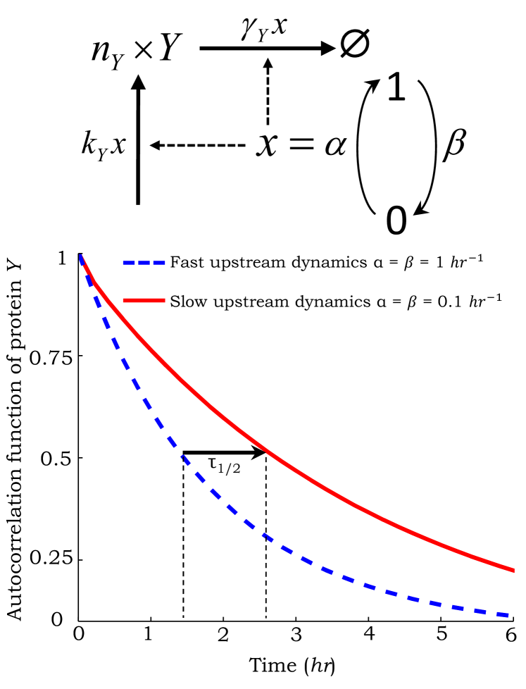
Figure 2: Autocorrelation in feedforward motif with biochemical switch. Top: Feedforward motif: both production and degradation rate of molecules $Y$ are dependent of upstream regulator $x$. Upstream process is restricted to the values $x=0$ and $x=1$. Its dynamics is governed by transition rates $(1-x)\alpha$ and $x\beta$. Bottom: $Y$-autocorrelation function as a function of the time. All the rates are normalized to protein decay rate, i.e., $\gamma_{Y}=1\ hr^{-1}$. Data are showing a shift of $\tau_{1/2}$ (time at which $R(t)$ reaches $50\%$ of its initial value) due to upstream regulator dynamics.

The autocorrelation function for different values of $\alpha$ and $\beta$ is shown in Fig. 2. One should note that $R(t)$ is independent of the creation process and its parameters $k_{Y}$ and ${\bar{b}_{Y}}$. It is however strongly dependent on the upstream process. Note that when taking the limit $\beta\rightarrow 0$ one recover the model with single protein for which $R(t)=\exp(-\gamma_{Y}t)$. It is particularly useful to define the ratio

$$\Gamma(t)=\frac{R(t)}{R(t)|_{\beta\rightarrow 0}},$$ (43)

for which we can show $\Gamma(t)\geq 1$ $\forall t$. In other words; the feedforward circuit leads to a systematic increase of the autocorrelation function. The increase of the time scale of fluctuations is therefore expected to lead to a larger noise values in further downstream products.

VI Effect of regulation in further downstream products

In this section we show that a signature of upstream input noise can be found in downstream products. We continue by considering the model, illustrated in Fig. 3, for which each molecule $Y$ can give birth to a burst of molecules $Z$. We write $k_{Z}$, $\bar{b}_{Z}$ and $\gamma_{Z}$ the associated creation rate, mean burst size and degradation rate. All transition rates are summarized in table V.

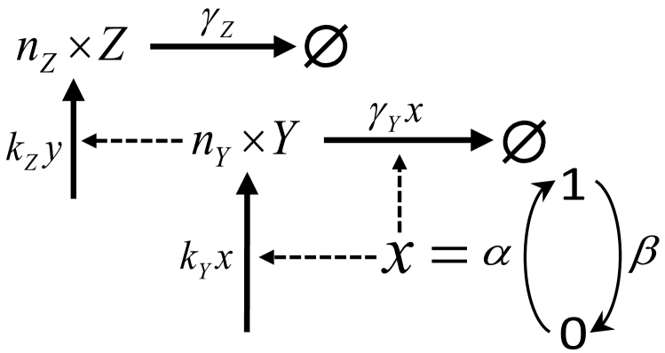
Figure 3: Schematic figure of a feedforward circuit regulated by a biological switch. $x$ is restricted to values $0$ and $1$ and governed by rates $\alpha$ and $\beta$. It affects both the production and degradation of Y, which itself activates production of downstream product $Z$. The creation and degradation rates of molecules $Y$ and $Z$ are denotes $k_{Y}$, $\gamma_{Y}$ and $k_{Z}$, $\gamma_{Z}$. Each creation event generates a burst, of size $n_{\bf j}$, characterized by a geometrical distribution $g(n_{\bf j}|\bar{b}_{\bf j})$ with mean ${\bar{b}_{\bf j}}$ (for ${\bf j}=Y,Z$).

Event	Reset	Transition rates
Switch activation	$x\rightarrow x+1$	$(1-x)\alpha$
Switch deactivation	$x\rightarrow x-1$	$x\beta$
burst of $n_{Y}$ $Y$ molecules	$y\rightarrow y+n_{Y}$	$xk_{Y}g(n_{Y}|{\bar{b}_{Y}})$
$Y$-degradation	$y\rightarrow y-1$	$xy\gamma_{Y}$
burst of $n_{Z}$ $Z$ molecules	$z\rightarrow z+n_{Z}$	$yk_{Z}g(n_{Z}|{\bar{b}_{Z}})$
$Z$-degradation	$z\rightarrow z-1$	$z\gamma_{Z}$

TABLE V: Transitions and associated rates for a feedforward model regulated by a biological switch.

Once again, to spare the readers patience, we choose not to write the full master equation. The reader could however convinced himself that the dynamics of regulator $X$ should leave a trace in downstream production. To proceed one could verify that the probability $P_{x,y,z}$ can not be written as product of marginal probabilities $Q_{x}\times R_{y,z}$. The generalized moment equation for this model is

$$\frac{d\langle x^{\sigma}y^{\eta}z^{\nu}\rangle}{dt} = (1-\delta_{\sigma,0})\left[\alpha\langle y^{\eta}z^{\nu}\rangle-(\alpha+\beta)\langle xy^{\eta}z^{\nu}\rangle\right]$$ (44)

$$+ k_{Y}\langle x^{\sigma+1}\left[(y+n_{Y})^{\eta}-y^{\eta}\right]z^{\nu}\rangle$$

$$+ \gamma_{Y}\langle x^{\sigma+1}\left[(y-1)^{\eta}-y^{\eta}\right]yz^{\nu}\rangle$$

$$+ k_{Z}\langle x^{\sigma}y^{\eta+1}\left[(z+n_{Z})^{\nu}-z^{\nu}\right]\rangle$$

$$+ \gamma_{Z}\langle x^{\sigma}y^{\eta}\left[(z-1)^{\nu}-z^{\nu}\right]z\rangle,$$

for $\sigma$, $\eta$ and $\nu$ integers and where $\delta_{\sigma,0}=1$ for $\sigma=0$ and zero otherwise. From the latter equation, (32) and (33) can be derived together with

$$\frac{d\langle z(t)\rangle}{dt} = k_{Z}\bar{b}_{Y}\langle y(t)\rangle-\gamma_{Z}\langle z(t)\rangle.$$ (45)

It follows that the stationary state is characterized by the mean numbers

$$\langle x\rangle=\frac{\alpha}{\alpha+\beta},\ \langle y\rangle=\frac{k_{Y}\bar{b}_{Y}}{\gamma_{Y}},\ \langle z\rangle=\frac{k_{Z}\bar{b}_{Z}}{\gamma_{Z}}\langle y\rangle.$$ (46)

We should note that both mean numbers $\langle y\rangle$ and $\langle z\rangle$ show no dependence on upstream regulation dynamics. However, we see that second order moment $\langle z^{2}\rangle$ is a function of the correlation term $\langle yz\rangle$:

$$\frac{d\langle z^{2}(t)\rangle}{dt} = 2k_{Z}\bar{b}_{Z}\langle yz(t)\rangle+k_{Z}(2\bar{b}_{Z}+1)\bar{b}_{Z}\langle y(t)\rangle$$ (47)

$$- 2\gamma_{Z}\langle z^{2}(t)\rangle+\gamma_{Z}\langle z(t)\rangle.$$

In the stationary state, the latter equation leads to

$$\langle z^{2}\rangle-\langle z\rangle^{2}=\langle z\rangle(1+{\bar{b}_{Z}})+\frac{k_{Z}{\bar{b}_{Z}}}{\gamma_{Z}}\left(\langle yz\rangle-\langle y\rangle\langle z\rangle\right).$$ (48)

To move forward we derive the moment equation for $\langle yz\rangle$:

$$\frac{d\langle yz(t)\rangle}{dt} = k_{Z}{\bar{b}_{Z}}\langle y^{2}(t)\rangle+k_{Y}{\bar{b}_{Y}}\langle xz(t)\rangle$$

$$- \gamma_{Z}\langle yz(t)\rangle-\gamma_{Y}\langle xyz(t)\rangle,$$

which, in the stationary state, becomes

$$\gamma_{Z}\langle yz\rangle+\gamma_{Y}\langle xyz\rangle=k_{Z}{\bar{b}_{Z}}\langle y^{2}\rangle+k_{Y}{\bar{b}_{Y}}\langle xz\rangle.$$ (50)

Along the same line, we derive equations for $d\langle xz\rangle/dt$ and $d\langle xyz\rangle/dt$. Taking the limit $t\rightarrow\infty$ leads to:

$$(\alpha+\beta+\gamma_{Z})\langle xz\rangle = \alpha\langle z\rangle+k_{Z}{\bar{b}_{Z}}\langle x\rangle\langle y\rangle.$$ (51)

$$(\alpha+\beta+\gamma_{Y}+\gamma_{Z})\langle xyz\rangle = \alpha\langle yz\rangle+k_{Y}{\bar{b}_{Y}}\langle xz\rangle$$ (52)

$$+ k_{Z}{\bar{b}_{Z}}\langle x\rangle\langle y^{2}\rangle.$$

The set of equation being close, we obtain the following steady-state coefficient of variation squared for $Z$

$$CV_{Z}^{2}=\frac{1+{\bar{b}_{Z}}}{\langle z\rangle}$$

$$+\frac{(1+{\bar{b}_{Y}})}{\langle y\rangle}\left\{1-\langle x\rangle\frac{\gamma_{Y}(\alpha+\beta+\gamma_{Z})}{(\alpha+\gamma_{Z})(\gamma_{Y}+\gamma_{Z})+\beta\gamma_{Z}}\right\}.$$

In the limit $\beta\rightarrow 0$ we have $\langle x\rangle=1$, leading to

$$CV_{Z}^{2}|_{\beta\rightarrow 0}=\frac{1+{\bar{b}_{Z}}}{\langle z\rangle}+\frac{\gamma_{Z}}{\gamma_{Y}+\gamma_{Z}}\frac{1+{\bar{b}_{Y}}}{\langle y\rangle}.$$ (54)

Note that the latter result is similar to (21) presented earlier in section III. It follows that the effect of the upstream regulation onto the noise in $Z$ downstream production can be quantified as:

$$CV_{Z}^{2}-CV_{Z}^{2}|_{\beta\rightarrow 0} = \frac{1+{\bar{b}_{Y}}}{\langle y\rangle}\frac{\gamma_{Y}}{\gamma_{Y}+\gamma_{Z}}(1-\langle x\rangle)$$ (55)

$$\times \frac{\gamma_{Z}(\alpha+\beta+\gamma_{Y}+\gamma_{Z})}{(\alpha+\gamma_{Z})(\gamma_{Y}+\gamma_{Z})+\beta\gamma_{Z}}.$$

Note that the difference $CV_{Z}^{2}-CV_{Z}^{2}|_{\beta\rightarrow 0}$ is always positive. Even if upstream noise has no direct effect on the distribution of $Y$ (and no effect on the mean number $\langle z\rangle$), this result shows that the feedforward motif leads to an increase of the noise $CV_{Z}^{2}$ in further downstream products.

The above results were illustrated for an upstream regulator $X$ modeled as a random switch, since exact analytical solutions for statistical moments were available. However, these results also hold qualitatively for a bursty birth-death process. In figure 4 we present noise measurements for the feedforward motif illustrated on figure 1, where $x(t)$ is a bursty birth-death process. These results are obtained by averaging a large number of Monte Carlo simulations performed using the Stochastic Simulation Algorithm [60]. Results confirm that $CV_{Y}^{2}$ is independent of the noise in $X$. Moreover it clearly shows an increase in downstream product noise $CV_{Z}^{2}$, with increasing noise in $X$.

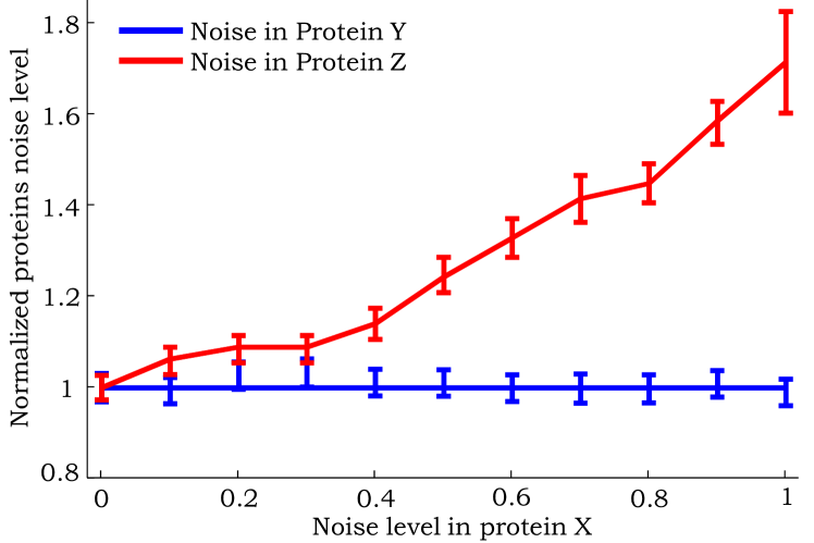
Figure 4: Noise levels in the molecular counts of $Y$ and $Z$ as a function of noise in the upstream regulator $X$ for circuit shown in Fig. 1. Noise in the levels of $X$ is changed by varying $k_{X}$ and $\bar{b}_{X}$ simultaneously but keeping the mean level $\langle x\rangle=100$ constant. Noise is quantified by the steady-state coefficient of variation squared and normalized with the respective noise levels for $CV^{2}_{X}=0$. All other parameters are fixed to $\gamma_{X}=\gamma_{Y}=\gamma_{Z}=1\ hr^{-1}$, $k_{Y}=10\ hr^{-1}$, $k_{Z}=20\ hr^{-1}$, and $\bar{b}_{Y}=\bar{b}_{Z}=1$.

VII Summary

Interesting features and new challenges are emerging from the study of biological systems regulated by upstream chemical processes and feedforward genetic motif. Our analysis started with a simple model describing a bursty production and single degradation of molecules $Y$. As expected, when the creation process is regulated by an upstream process, a clear signature of the input noise $X$ is seen in both first (19) and second order moments (21) of the $Y$-distribution. However, when upstream regulation comes to affect both creation and degradation process, forming a feedforward circuit, we were able to show that all $x$-$y$ correlations vanishes. Thus, the feedforward regulation completely buffers $Y$ from random fluctuations in the upstream regulator and $x$ appears as a ”hidden” variable. We show that a first signature of the existence of $x$ can be found in dynamical quantities. The autocorrelation function was calculated exactly for a feedforward circuit regulated by a simple switch (V-B). Our results show dependence in the switch activity and a systematic increase of correlation time scales (43). Interestingly, an indication of noise in upstream regulatory processes can be found in the distribution of further downstream products (VI). Here we have shown that the feedforward motif leads to an increase of noise in downstream product (55) leaving however the mean count of molecules $\langle z\rangle$ invariant. In addition, identical observations were confirmed by Monte Carlo simulations (see figure 4) of the more sophisticated model with bursty creation and single degradation of $X$.

The incoherent feedforward circuit considered here is highly simplified, and in reality these systems often involve often biochemical species. For example, instead of $X$ directly activating the production of $Y$, it activates it via an intermediate specie [45]. One way to incorporate such intermediate species is by introducing time delays. In future work we will investigate stochastic dynamic of circuits where the regulatory effects of $X$ on $Y$ are time delayed. The delays could come in either activation or degradation, and the delay itself could be a random variable.

References

- [1] A. Raj and A. van Oudenaarden, “Nature, nurture, or chance: stochastic gene expression and its consequences,” Cell, vol. 135, pp. 216–226, 2008.
- [2] W. J. Blake, M. Kaern, C. R. Cantor, and J. J. Collins, “Noise in eukaryotic gene expression,” Nature, vol. 422, pp. 633–637, 2003.
- [3] J. M. Raser and E. K. O’Shea, “Noise in gene expression: Origins, consequences, and control,” Science, vol. 309, pp. 2010 – 2013, 2005.
- [4] M. Kærn, T. C. Elston, W. J. Blake, and J. J. Collins, “Stochasticity in gene expression: from theories to phenotypes,” Nature Reviews Genetics, vol. 6, pp. 451–464, 2005.
- [5] A. Eldar and M. B. Elowitz, “Functional roles for noise in genetic circuits,” Nature, vol. 467, pp. 167–173, 2010.
- [6] G. Neuert, B. Munsky, R. Z. Tan, L. Teytelman, M. Khammash, and A. van Oudenaarden, “Systematic identification of signal-activated stochastic gene regulation,” Science, vol. 339, pp. 584–587, 2013.
- [7] G. Chalancon, C. N. Ravarani, S. Balaji, A. Martinez-Arias, L. Aravind, R. Jothi, and M. Babu, “Interplay between gene expression noise and regulatory network architecture,” Trends in Genetics, vol. 28, pp. 221–232, 2012.
- [8] A. Magklara and S. Lomvardas, “Stochastic gene expression in mammals: lessons from olfaction,” Trends in Cell Biology, vol. 23, pp. 449–456, 2014.
- [9] D. L. Jones, R. C. Brewster, and R. Phillips, “Promoter architecture dictates cell-to-cell variability in gene expression,” Science, vol. 346, pp. 1533–1536, 2014.
- [10] E. Libby, T. J. Perkins, and P. S. Swain, “Noisy information processing through transcriptional regulation,” Proceedings of the National Academy of Sciences, vol. 104, pp. 7151–7156, 2007.
- [11] H. B. Fraser, A. E. Hirsh, G. Giaever, J. Kumm, and M. B. Eisen, “Noise minimization in eukaryotic gene expression,” PLOS Biology, vol. 2, p. e137, 2004.
- [12] B. Lehner, “Selection to minimise noise in living systems and its implications for the evolution of gene expression,” Molecular Systems Biology, vol. 4, p. 170, 2008.
- [13] R. Kemkemer, S. Schrank, W. Vogel, H. Gruler, and D. Kaufmann, “Increased noise as an effect of haploinsufficiency of the tumor-suppressor gene neurofibromatosis type 1 in vitro,” Proceedings of the National Academy of Sciences, vol. 99, pp. 13 783–13 788, 2002.
- [14] D. L. Cook, A. N. Gerber, and S. J. Tapscott, “Modeling stochastic gene expression: implications for haploinsufficiency,” Proceedings of the National Academy of Sciences, vol. 95, pp. 15 641–15 646, 1998.
- [15] R. Bahar, C. H. Hartmann, K. A. Rodriguez, A. D. Denny, R. A. Busuttil, M. E. Dolle, R. B. Calder, G. B. Chisholm, B. H. Pollock, C. A. Klein, and J. Vijg, “Increased cell-to-cell variation in gene expression in ageing mouse heart,” Nature, vol. 441, pp. 1011–1014, 2006.
- [16] A. Brock, H. Chang, and S. Huang, “Non-genetic heterogeneity – a mutation-independent driving force for the somatic evolution of tumours,” Nature Reviews Genetics, vol. 10, pp. 336–342, 2009.
- [17] A. P. Arkin, J. Ross, and H. H. McAdams, “Stochastic kinetic analysis of developmental pathway bifurcation in phage -infected Escherichia coli cells,” Genetics, vol. 149, pp. 1633–1648, 1998.
- [18] R. Losick and C. Desplan, “Stochasticity and cell fate,” Science, vol. 320, pp. 65–68, 2008.
- [19] G. Balázsi, A. van Oudenaarden, and J. J. Collins, “Cellular decision making and biological noise: From microbes to mammals,” Cell, vol. 144, pp. 910–925, 2014.
- [20] T. M. Norman, N. D. Lord, J. Paulsson, and R. Losick, “Memory and modularity in cell-fate decision making,” Nature, vol. 503, pp. 481–486, 2013.
- [21] F. St-Pierre and D. Endy, “Determination of cell fate selection during phage lambda infection,” Proceedings of the National Academy of Sciences, vol. 105, pp. 20 705–20 710, 2008.
- [22] K. H. Kim and H. M. Sauro, “Adjusting phenotypes by noise control,” PLOS Computational Biology, vol. 8, p. e1002344, 2012.
- [23] H. H. Chang, M. Hemberg, M. Barahona, D. E. Ingber, and S. Huang, “Transcriptome-wide noise controls lineage choice in mammalian progenitor cells,” Nature, vol. 453, pp. 544–547, 2008.
- [24] E. Abranches, A. M. V. Guedes, M. Moravec, H. Maamar, P. Svoboda, A. Raj, and D. Henrique, “Stochastic nanog fluctuations allow mouse embryonic stem cells to explore pluripotency,” Development, vol. 141, pp. 2770–2779, 2014.
- [25] M. E. Torres-Padilla and I. Chambers, “Transcription factor heterogeneity in pluripotent stem cells: a stochastic advantage,” Development, vol. 141, pp. 2173–2181, 2014.
- [26] L. S. Weinberger, J. Burnett, J. Toettcher, A. Arkin, and D. Schaffer, “Stochastic gene expression in a lentiviral positive-feedback loop: HIV-1 Tat fluctuations drive phenotypic diversity,” Cell, vol. 122, pp. 169–182, 2005.
- [27] L. S. Weinberger, R. D. Dar, and M. L. Simpson, “Transient-mediated fate determination in a transcriptional circuit of HIV,” Nature Genetics, vol. 40, pp. 466 – 470, 2008.
- [28] R. L. Thompson, C. M. Preston, and N. M. Sawtell, “De novo synthesis of VP16 coordinates the exit from HSV latency in vivo,” PLOS Pathogens, vol. 5, p. e1000352, 2009.
- [29] A. Singh and L. S. Weinberger, “Stochastic gene expression as a molecular switch for viral latency,” Current Opinion in Microbiology, vol. 12, pp. 460–466, 2009.
- [30] H. El-Samad and M. Khammash, “Regulated degradation is a mechanism for suppressing stochastic fluctuations in gene regulatory networks,” Biophysical Journal, vol. 90, pp. 3749–3761, 2006.
- [31] A. Singh and J. P. Hespanha, “Evolution of autoregulation in the presence of noise,” IET Systems Biology, vol. 3, pp. 368–378, 2009.
- [32] I. Lestas, G. Vinnicombegv, and J. Paulsson, “Fundamental limits on the suppression of molecular fluctuations,” Nature, vol. 467, pp. 174–178, 2010.
- [33] P. S. Swain, “Efficient attenuation of stochasticity in gene expression through post-transcriptional control,” Journal of Molecular Biology, vol. 344, pp. 956–976, 2004.
- [34] G. Balazsi, A. P. Heath, L. Shi, and M. L. Gennaro, “The temporal response of the mycobacterium tuberculosis gene regulatory network during growth arrest,” Molecular Systems Biology, vol. 4, p. 225, 2008.
- [35] M. A. Savageau, “Comparison of classical and autogenous systems of regulation in inducible operons,” Nature, vol. 252, pp. 546–549, 1974.
- [36] A. Becskei and L. Serrano, “Engineering stability in gene networks by autoregulation,” Nature, vol. 405, pp. 590–593, 2000.
- [37] D. Nevozhay, R. M. Adams, K. F. Murphy, K. Josic, and G. Balazsi, “Negative autoregulation linearizes the dose response and suppresses the heterogeneity of gene expression,” Proceedings of the National Academy of Sciences, vol. 106, pp. 5123–5128, 2009.
- [38] Y. Dublanche, K. Michalodimitrakis, N. Kummerer, M. Foglierini, and L. Serrano, “Noise in transcription negative feedback loops: simulation and experimental analysis,” Molecular Systems Biology, vol. 2, p. 41, 2006.
- [39] M. Thattai and A. van Oudenaarden, “Intrinsic noise in gene regulatory networks,” Proceedings of the National Academy of Sciences, vol. 98, pp. 8614–8619, 2001.
- [40] A. Singh and J. P. Hespanha, “Optimal feedback strength for noise suppression in autoregulatory gene networks,” Biophysical Journal, vol. 96, pp. 4013–4023, 2009.
- [41] D. Orrell and H. Bolouri, “Control of internal and external noise in genetic regulatory networks,” Journal of Theoretical Biology, vol. 230, pp. 301–312, 2004.
- [42] A. Singh and J. P. Hespanha, “Stochastic analysis of gene regulatory networks using moment closure,” in Proc. of the 2007 Amer. Control Conference, New York, NY, 2006.
- [43] B. Hu, D. A. Kessler, W.-J. Rappel, and H. Levine, “Effects of input noise on a simple biochemical switch,” Physical Review Letters, vol. 107, p. 148101, 2011.
- [44] L. Bleris, Z. Xie, D. Glass, A. Adadey, E. Sontag, and Y. Benenson, “Synthetic incoherent feedforward circuits show adaptation to the amount of their genetic template,” Molecular Systems Biology, vol. 7, p. 519, 2011.
- [45] U. Alon, “Network motifs: theory and experimental approaches,” Nature Reviews Genetics, vol. 8, pp. 450–461, 2007.
- [46] M. E. Wall, W. S. Hlavacek, and M. A. Savageau, “Design principles for regulator gene expression in a repressible gene circuit,” Journal of Molecular Biology, vol. 332, pp. 861–876, 2003.
- [47] J. Tsang, J. Zhu, and A. van Oudenaarden, “MicroRNA-mediated feedback and feedforward loops are recurrent network motifs in mammals,” Molecular Cell, vol. 26, pp. 753–767, 2007.
- [48] V. Shahrezaei and P. S. Swain, “Analytical distributions for stochastic gene expression,” Proceedings of the National Academy of Sciences, vol. 105, pp. 17 256–17 261, 2008.
- [49] J. Paulsson, “Model of stochastic gene expression,” Physics of Life Reviews, vol. 2, pp. 157–175, 2005.
- [50] A. Singh and M. Soltani, “Quantifying intrinsic and extrinsic variability in stochastic gene-expression models,” PLOS ONE, vol. 8, p. e84301, 2013.
- [51] D. T. Gillespie, “A general method for numerically simulating the stochastic time evolution of coupled chemical reactions,” Journal of Computational Physics, vol. 22, pp. 403–434, 1976.
- [52] D. A. McQuarrie, “Stochastic approach to chemical kinetics,” Journal of Applied Probability, vol. 4, pp. 413–478, 1967.
- [53] D. J. Wilkinson, Stochastic Modelling for Systems Biology. Chapman and Hall/CRC, 2011.
- [54] A. Singh and J. P. Hespanha, “Approximate moment dynamics for chemically reacting systems,” IEEE Transactions on Automatic Control, vol. 56, pp. 414–418, 2011.
- [55] ——, “Stochastic hybrid systems for studying biochemical processes,” Philosophical Transactions of the Royal Society A, vol. 368, pp. 4995–5011, 2010.
- [56] A. Singh and P. Bokes, “Consequences of mRNA transport on stochastic variability in protein levels,” Biophysical Journal, vol. 103, pp. 1087–1096, 2012.
- [57] M. Soltani, P. Bokes, Z. Fox, and A. Singh, “Nonspecific transcription factor binding can reduce noise in the expression of downstream proteins,” Physical Biology, vol. 12, p. 055002, 2015.
- [58] J. P. Hespanha and A. Singh, “Stochastic models for chemically reacting systems using polynomial stochastic hybrid systems,” International Journal of Robust and Nonlinear Control, vol. 15, pp. 669–689, 2005.
- [59] H. Pendar, T. Platini, and R. V. Kulkarni, “Exact protein distributions for stochastic models of gene expression using partitioning of poisson processes,” Physical Review. E, vol. 87, p. 042720, 2013.
- [60] D. T. Gillespie, “Approximate accelerated stochastic simulation of chemically reacting systems,” Journal of Chemical Physics, vol. 115, pp. 1716–1733, 2001.