Loop quantum cosmology and the fate of cosmological singularities

Abstract

Singularities in general relativity such as the big bang and big crunch, and exotic singularities such as the big rip are the boundaries of the classical spacetimes. These events are marked by a divergence in the curvature invariants and the breakdown of the geodesic evolution. Recent progress on implementing techniques of loop quantum gravity to cosmological models reveals that such singularities may be generically resolved because of the quantum gravitational effects. Due to the quantum geometry, which replaces the classical differential geometry at the Planck scale, the big bang is replaced by a big bounce without any assumptions on the matter content or any fine tuning. In this manuscript, we discuss some of the main features of this approach and the results on the generic resolution of singularities for the isotropic as well as anisotropic models. Using effective spacetime description of the quantum theory, we show the way quantum gravitational effects lead to the universal bounds on the energy density, the Hubble rate and the anisotropic shear. We discuss the geodesic completeness in the effective spacetime and the resolution of all of the strong singularities. It turns out that despite the bounds on energy density and the Hubble rate, there can be divergences in the curvature invariants. However such events are geodesically extendible, with tidal forces not strong enough to cause inevitable destruction of the in-falling objects.

1 Introduction

Einstein’s theory of general relativity is extremely successful in describing the evolution of our universe from the early stages to the very large scales. However, it suffers from the problem of classical singularities which are the generic features of spacetimes in general relativity. In the cosmological context, a spatially flat Friedmann-Lemaître-Robertson-Walker (FLRW) spacetime filled with matter with an equation of state such as of dust, radiation, a stiff fluid or even an inflaton, evolves from a big bang singularity in the past where the scale factor vanishes. If the universe is contracting, then for these types of matter, evolution ends in a big crunch singularity in a finite future. The physics of these singularities is very rich. First, let us note that in general not all singularities occur at a vanishing scale factor. A singularity may occur even at an infinite value of the scale factor, such as in the big rip, or at a finite value of the scale factor such as in the sudden and big freeze singularities. Further, singularities come in different strengths and they can be strong or weak (Ellis & Schmidt, 1977; Clarke & Królak, 1985; Tipler, 1977; Krolak, 1986). Strong singularities are identified by the tidal forces which are infinite, causing inevitable destruction of any in-falling object with arbitrary characteristics. Weak singularities on the other hand can have divergence in the spacetime curvature, but they are not strong enough to destroy arbitrary in-falling detectors. Big bang and big rip are examples of the strong singularities where geodesic evolution breaks down and hence these are the boundaries of classical spacetime. Examples of weak singularities include sudden singularities, beyond which geodesics can be extended. In the presence of anisotropies, such as in the Bianchi-I model, singularities come in different ‘shapes.’ (Doroshkevich, 1965; Thorne, 1967; Ellis, 1967; Ellis & MacCallum, 1969; Jacobs, 1968). Unlike the point like big bang/big crunch singularity in the isotropic cosmological models, in the presence of anisotropies the singularities can also be a cigar, barrel, and a pancake like depending on the behavior of directional scale factors. If the spatial curvature is present in addition, the approach to classical singularities oscillatory and leads to the mixmaster dynamics (Berger, 2002; Garfinkle, 2007).

The existence of singularities, such as the big bang, shows that classical general relativity reaches its limits of validity when the spacetime curvature becomes extremely large, and in such a case gravitational physics should be described by a quantum theory of gravity. One of the main attempts to quantize gravity is loop quantum gravity, which is a non-perturbative canonical quantization of gravity based on Ashtekar variables (Ashtekar & Lewandowski, 2004; Rovelli, 2004; Thiemann, 2007; Gambini & Pullin, 2011). Though a full theory of loop quantum gravity is not yet available, it has reached a high mathematical precision and various important results have been obtained. A key prediction of loop quantum gravity is that classical differential geometry of general relativity is replaced by a quantum geometry at the Planck scales. For spacetimes with symmetries, such as the cosmological and black hole spacetimes, techniques of loop quantum gravity have been used to perform a rigorous quantization and detailed physical implications have been studied. In this manuscript we focus on the applications of these techniques to cosmological models in loop quantum cosmology, where isotropic and anisotropic models have been widely investigated, and recently these techniques have been used to study the effects of quantum gravity in the inhomogeneous situations, including Gowdy models (Martin-Benito, Garay & Marugan, 2008; Garay et al., 2010; Brizuela et al., 2010) and quantum fluctuations in loop quantized spacetime (Agullo, Ashtekar & Nelson, 2013a, b). Loop quantization of black hole spacetimes, a discussion of which falls beyond the scope of this manuscript, uses similar techniques as in loop quantum cosmology, and leads to similar results on singularity resolution (Ashtekar & Bojowald, 2006; Gambini & Pullin, 2008, 2013).

Loop quantum cosmology carries forward the quantum cosmology program which started from the canonical quantization of cosmological spacetimes in the metric variables. In the metric based formulation of quantum cosmology, the Wheeler-DeWitt quantum cosmology, resolution of singularities remains problematic. The spacetime in Wheeler-DeWitt quantization is a continuum as in the classical general relativity and strong singularities are present in general unless one chooses very special boundary conditions. In a sharp contrast, the underlying geometry in loop quantum cosmology is a discrete quantum geometry inherited from loop quantum gravity. Instead of the differential equation which governs the evolution in the Wheeler-DeWitt theory, in loop quantum cosmology, evolution operator is a discrete quantum operator (Bojowald, 2001; Ashtekar, Bojowald & Lewandowski, 2003). It is only at the large scales compared to the Planck scale, that the discrete quantum geometry is approximated by the classical differential geometry, and there is an agreement between the physical implications of loop quantum cosmology and the Wheeler-DeWitt theory. However, in the Planck regime there are significant and striking differences between Wheeler-DeWitt theory and loop quantum cosmology. A sharply peaked state on a classical trajectory when evolved towards the big bang in the Wheeler-DeWitt theory, follows the classical trajectory all the way to the classical singularity. In loop quantum cosmology, such a state bounces when energy density reaches a maximum value $\rho_{\rm max}\approx 0.41\rho_{\rm{Pl}}$ (Ashtekar et al., 2006a, b, c). The occurrence of bounce which, first observed in the loop quantized spatially flat FLRW model with a massless scalar field, occurs without any violation of the energy conditions or fine tuning. The physics of the bounce has been found to be robust using an exactly solvable model (Ashtekar, Corichi, & Singh, 2008). The quantum probability for the bounce turns out to be unity (Craig & Singh, 2013). Following the method for the spatially flat model, loop quantization has been carried out for different matter models and in the presence of spatial curvature in homogeneous spacetimes (Ashtekar et al., 2007; Szulc et al., 2007; Bentivegna & Pawlowski, 2008; Pawlowski, Ashtekar, 2012; Corichi & Karami, 2014; Pawlowski et al., 2014; Ashtekar et al., 2014; Diener et al., 2014c). The existence of bounce is a generic result in all these investigations. The states remain sharply peaked throughout the non-singular evolution and quantum fluctuations are tightly constrained across the bounce (Corichi & Singh, 2008a; Kaminski & Pawlowski, 2010b; Corichi & Montoya, 2011). The quantum resolution of big bang singularity is not confined only to the isotropic models. The quantum evolution operator in anisotropic models, such as the Bianchi-I, Bianchi-II and Bianchi-IX models, has been shown to be non-singular (Chiou, 2007; Martin-Benito, Marugan, Pawlowski, 2009; Ashtekar & Wilson-Ewing, 2009a, b; Wilson-Ewing, 2010; Singh & Wilson-Ewing, 2014). In case of the infinite degrees of freedom, Gowdy models have been recently studied. Though these models are not yet fully loop quantized, important insights on the nature of bounce have been obtained (Martin-Benito, Garay & Marugan, 2008; Garay et al., 2010; Brizuela et al., 2010).

An important feature of loop quantum cosmology is the effective spacetime description of the underlying quantum evolution. For the states which lead to a classical macroscopic universe at late times, this description can be obtained from an effective Hamiltonian (Willis, 2004; Taveras, 2008). Rigorous numerical simulations have confirmed the validity of the effective dynamics (Ashtekar et al., 2006c, 2007; Bentivegna & Pawlowski, 2008; Pawlowski, Ashtekar, 2012; Diener et al., 2014a), which provides an excellent approximation to the full loop quantum dynamics for the sharply peaked states at all the scales. It has been shown that only when the states have very large quantum fluctuations at late times, i.e. they do not lead to macroscopic universes described by general relativity, that the effective dynamics has departures from the quantum dynamics near bounce and the subsequent evolution (Diener et al., 2014a, b). In such a case, the effective dynamics overestimates the density at the bounce, but still captures the qualitative aspects extremely well. The effective dynamics approach has been extensively used to study physics at the Planck scale and the very early universe in loop quantum cosmology (see Ashtekar & Singh (2011) for various applications of the effective theory). Some of the applications include non-singular inflationary attractors in isotropic (Singh, Vandersloot & Vereshchagin, 2006; Ashtekar & Sloan, 2011; Ranken & Singh, 2012) and anisotropic models (Gupt & Singh, 2013), and the probability of inflation to occur (Ashtekar & Sloan, 2011, 2010; Corichi & Karami, 2011; Corichi & Sloan, 2013), transitions between non-singular geometrical structures in the Bianchi-I model (Gupt & Singh, 2012), singularity resolution in string cosmology inspired (de Risi, Maartens & Singh, 2007; Cailleteau et al., 2009), and multiverse scenarios (Garriga, Vilenin & Zhang, 2013; Gupt & Singh, 2014), and various studies on cosmological perturbations (see Barrau et al. (2014) for a review).

An interesting application of effective dynamics is to study the fate of singularities in general for different matter models. The idea is based on analyzing the generic properties of curvature invariants, geometric scalars such expansion and shear scalars, and the geodesic evolution in the effective spacetime. This approach leads to some striking results. Assuming the validity of the effective dynamics, one finds that for generic matter with arbitrary equation of state, the effective spacetime in the spatially flat model is geodesically complete, and there are no strong curvature singularities (Singh, 2009). Loop quantum cosmology resolves all the singularities such as big bang, big rip and big freeze (Singh, 2009; Sami et al., 2006; Samart & Gumjudpai, 2007; Naskar & Ward, 2007), but interestingly ignores the sudden singularities (Cailleteau et al., 2008; Singh, 2009). It is interesting to note that quantum geometric effects are able to differentiate between genuine and the harmless singularities, and only resolve the former types. These results hold for the case when spatial curvature is present, where resolution of strong singularities and non-resolution of weak singularities has been confirmed via a phenomenological analysis (Singh & Vidotto, 2011). Generalization of this analysis has been performed in the presence of anisotropies where it has been shown that all strong singularities which occur in classical general relativity in the Bianchi-I spacetime are avoided, and the geodesic evolution does not break down in general (Singh, 2012). These results are tied to the universal bounds on the energy density, expansion scalar (or the mean Hubble rate), and shear scalar in the effective spacetime of loop quantum cosmology for the isotropic and Bianchi-I model (Singh, 2012; Corichi & Singh, 2009). Recently, similar bounds on geometric scalars have been obtained for the Bianchi-II (Gupt & Singh, 2012), Bianchi-IX (Singh & Wilson-Ewing, 2014) and Kantowski-Sachs spacetime (Joe & Singh, 2014), which indicates that these conclusions can be generalized to other anisotropic models and black hole spacetimes.

In this manuscript, we give an overview of the main result of the bounce, and the generic resolution of singularities using effective spacetime description in loop quantum cosmology. To make this manuscript self contained with basic techniques, in Sec. 2 we summarize concepts in the classical theory which are needed for discussion in the later sections. Loop quantum cosmology is a canonical quantization involving a $3+1$ decomposition of the spacetime. This decomposition and the Hamiltonian framework is summarized in the first part of Sec. 2. We express the Einstein-Hilbert action in terms of the quantities defined with respect to the three dimensional spatial slices, and obtain constraints both in the metric variables and Ashtekar variables in the classical theory. We then implement these techniques to obtain a Hamiltonian formulation of the spatially flat FLRW spacetime and show the way classical field equations, such as the Friedmann equation, can be obtained from the Hamiltonian constraint and the Hamilton’s equation. In Sec. 2.3 and 2.4, we discuss geodesic evolution, strength and different types of singularities. Though these are discussed in the isotropic setting, the same classifications apply to the anisotropic spacetime. In Sec. 3, we provide a short summary of the loop quantization of the spatially flat homogeneous and isotropic model in loop quantum cosmology. We discuss the way quantum geometric effects lead to a discrete quantum evolution equation which avoids the singularity, and leads to the quantum bounce of the universe at the Planck scale. Sec. 4 deals with the effective spacetime description and application of this method to understand bounds on Hubble rate, curvature scalars, geodesic completeness and the absence of strong curvature singularities. A discussion of these results to an anisotropic spacetime, the Bianchi-I model, is provided in Sec. 5. We conclude with a brief discussion of the main results in Sec. 6. Due to the space constraints, it is is not possible to cover all the details and developments in this manuscript, especially various conceptual issues and the progress in numerical methods which have provided valuable insights and served as robustness tests on singularity resolution. An interested reader may refer to reviews, such as Ashtekar & Lewandowski (2004) and Ashtekar & Singh (2011) for details on loop quantum gravity and loop quantum cosmology respectively. The numerical techniques used in loop quantum cosmology are reviewed in detail in Singh (2012) and Brizuela et al. (2012).

2 Classical theory: Hamiltonian framework and and the properties of singularities

In this section, we overview some aspects of the classical theory which are useful to understand the underlying procedure of quantization of cosmological spacetimes in loop quantum cosmology, and the properties of singularities. We start with the $3+1$ decomposition of the classical spacetime and discuss the way Hamiltonian and diffeomorphism constraints arise in the metric variables and the Ashtekar variables. We then specialize to the case of the spatially flat homogeneous and isotropic model, where due to the symmetries the diffeomorphism constraint is satisfied, and the only non-trivial constraint is the Hamiltonian constraint. Using Hamilton’s equations, we demonstrate the way classical Friedmann equation can be derived in this setting. In the last part of this section, we discuss the properties of geodesics and different types of singularities in the classical theory for the $k=0$ FLRW spacetime.

2.1 The 3+1 decomposition and constraints

Loop quantum gravity is a canonical quantization of gravity based on a $3+1$ decomposition of a spacetime manifold. Let us consider the topology of the spacetime with metric $g_{ab}$ as $\Sigma\times R$. If there exists a global time $t$, then the spacetime can be foliated into constant time hypersurfaces $\Sigma$, each with a spatial metric

$$q_{ab}=g_{ab}+n_{a}n_{b}\leavevmode\nobreak\ ,$$ (1)

where $n_{a}$ is a unit normal to the hypersurface $\Sigma$. Using it, a time-like vector field $t^{\mu}$ can be decomposed into normal and tangential components to the spatial slices $\Sigma$ as $t^{a}=Nn^{a}+N^{a}$, where $N$ is the lapse and $N^{a}$ denotes the shift vector. In the Hamiltonian formulation of general relativity in the metric variables, $q_{ab}$ acts as the configuration variable. Its conjugate variable is $\pi^{ab}=\sqrt{q}(K^{ab}-Kq^{ab})$, where $q$ denotes the determinant of the spatial metric, and $K_{ab}$ is the extrinsic curvature of the spacetime defined as $K_{ab}=-q_{a}^{c}\nabla_{c}n_{a}$.

Using the $3+1$ decomposition, the Einstein-Hilbert action for general relativity can be expressed as

$$S = \int{\rm d}^{4}x\sqrt{-g}R$$ (2)

$$= \int{\rm d}^{4}x\left(\pi^{ab}\dot{q}_{ab}+N\sqrt{q}\left({}^{(3)}R-q^{-1}(\pi^{cd}\pi_{cd}+\frac{1}{2}(\pi^{i}_{i})^{2})\right)+2N_{a}\sqrt{q}D_{b}(\sqrt{q}\pi^{ab})\right)\leavevmode\nobreak\ ,$$

where $D_{a}$ denotes the 3-dimensional covariant derivative. Note that the Lagrangian does not contain any time derivatives of the lapse $N$ and the shift vector $N_{a}$. Therefore, these act as Lagrange multipliers, variations with respect to which yield us the constraints:

$${\cal C}_{H}=-{}^{(3)}R+q^{-1}(\pi^{ab}\pi_{ab}-\frac{1}{2}(\pi^{i}_{i})^{2})=0$$ (3)

and

$${\cal C}_{D}^{a}=D_{b}(\sqrt{q}\pi^{ab})=0\leavevmode\nobreak\ .$$ (4)

Here $C_{H}$ is the Hamiltonian constraint and $C_{D}^{a}$ is the spatial diffeomorphism constraint. The total Hamiltonian is the sum of these constraints: ${\cal H}=\int{\rm d}^{3}x(N{\cal C}_{H}+N_{a}{\cal C}^{a})$. The form of the Hamiltonian in the metric variables makes it very difficult to obtain physical solutions in the quantum theory. Nevertheless, for spacetimes with symmetries, such as homogeneous cosmological spacetimes, one can quantize the Hamiltonian and obtain physical states. This metric based approach to quantize cosmological spacetimes is known as the Wheeler-DeWitt quantum cosmology, some aspects of which will be discussed in the next section.

The Hamiltonian constraint becomes simpler to handle in the Ashtekar variables (Ashtekar, 1986): the connection $A^{i}_{a}$ and the (densitized) triad $E^{a}_{i}$, where $a$ and $i$ are the spatial and internal indices respectively, taking vales 1,2,3. The spatial metric on $\Sigma$ can be constructed using triads as,

$$E^{a}_{i}E^{b}_{j}\delta^{ij}=|q|q^{ab}\leavevmode\nobreak\ .$$ (5)

The connection is related to the time derivative of the metric, and can be written in terms of the extrinsic curvature as

$$A^{i}_{a}=\Gamma^{i}_{a}+\gamma K^{i}_{a}\leavevmode\nobreak\ ,$$ (6)

where $\gamma\approx 0.2375$ is the Barbero-Immirzi parameter whose value is fixed in loop quantum gravity using black hole thermodynamics, $K_{a}^{i}=K_{ab}E^{ai}/\sqrt{|q|}$, and $\Gamma^{i}_{a}$ is the spin connection:

$$\Gamma^{i}_{a}=-\frac{1}{2}\epsilon^{ijk}e_{j}^{b}(\partial_{a}e_{b}^{k}-\partial_{b}e_{a}^{k}+\delta_{mn}e_{k}^{l}e_{a}^{m}\partial_{l}e_{b}^{n})$$ (7)

where $e^{a}_{i}=E^{a}_{i}/\sqrt{|q|}$, and $e^{a}_{i}e_{a}^{j}=\delta^{j}_{i}$.

Rewriting the Einstein-Hilbert action in terms of the Ashtekar variables, one obtains the following constraints:

$$D_{a}E^{a}_{i}=0,\leavevmode\nobreak\ \leavevmode\nobreak\ \leavevmode\nobreak\ \leavevmode\nobreak\ \leavevmode\nobreak\ \leavevmode\nobreak\ E^{a}_{i}F_{ab}^{i}=0$$ (8)

and

$$\frac{1}{\sqrt{|q|}}E^{a}_{j}E^{b}_{k}(\epsilon_{i}^{jk}F_{ab}^{i}-(1+\gamma^{2})(K^{j}_{a}K_{b}^{k}-K^{j}_{b}K_{a}^{k}))=0\leavevmode\nobreak\ .$$ (9)

The first constraint is the Gauss constraint, the second is the momentum constraint and the third constraint is the Hamiltonian constraint. Here the latter two are obtained by imposing the Gauss constraint. The Gauss and the momentum constraints can be combined to give the diffeomorphism constraint. Once we have the Hamiltonian as the linear combination of the constraints, we can obtain dynamical equations from the Hamilton’s equations which along with the constraint equations yield us an equivalent formulation of the Einstein field equations. In the quantum theory, the physical states are those which are annihilated by the operator corresponding to quantum Hamiltonian. These states constitute the physical Hilbert space of the quantized gravitational spacetime.

We conclude this part by noting a conceptual difficulty in the Hamiltonian framework. Since the Hamiltonian is a linear combination of the constraints, it (weakly) vanishes, and hence the dynamics is frozen. In the quantum theory, the genuine observables commute with the Hamiltonian, and thus they do not evolve. This is the problem of time, which can be addressed using relational dynamics by defining observables which provide us relations between different dynamical quantities. An example of the relational dynamics is using a matter field $\phi$ as a clock to measure the way gravitational degrees of freedom change. We discuss one such example in the spatially flat isotropic and homogeneous spacetime with a massless scalar field in the following.

2.2 The spatially flat, homogeneous and isotropic spacetime: from Hamiltonian to Friedmann equation

Let us illustrate the Hamiltonian constraint and how it can be used to obtain classical dynamical equations for the the spatially flat isotropic and homogeneous FLRW spacetime. The metric for lapse $N=1$ is given by

$${\rm d}s^{2}=-\,{\rm d}t^{2}\,+q_{ab}{\rm d}x^{a}{\rm d}x^{b}=-{\rm d}t^{2}+a^{2}\left(dr^{2}+r^{2}\left(d\theta^{2}+\sin^{2}\theta d\phi^{2}\right)\right)$$ (10)

where $a(t)$ is the scale factor of the universe, and $t$ is the proper time. The extrinsic curvature of the spacetime turns out to be $K_{ab}=(\dot{a}/a)q_{ab}$. In the metric variables, the gravitational phase space variables are $a$ and $p_{a}$, which satisfy: $\{a,p_{a}\}=4\pi G/3$. If the matter source is a massless scalar field $\phi$, then the matter phase space variables are $\phi$ and its conjugate $p_{\phi}$, which satisfy $\{\phi,p_{\phi}\}=1$. Due to the homogeneity of the FLRW spacetime, the spatial diffeomorphism constraint is trivially satisfied, and one is left with the Hamiltonian constraint, given by

$${C_{H}}^{\rm{(cl)}}=-\frac{3}{8\pi G}\frac{p_{a}^{2}}{a}+\frac{p_{\phi}^{2}}{2a^{3}}\leavevmode\nobreak\ ,$$ (11)

(where we have introduced the superscript ${\mathrm{(cl)}}$ to distinguish the Hamiltonian constraint in the classical theory from the later occurrences).

Using Hamilton’s equations, we can relate the conjugate momenta $p_{a}$ and $p_{\phi}$ with $a$ and $\phi$ respectively. It is straightforward to see that $p_{a}$ is related to the time derivative of the scale factor as

$$\dot{a}=\{a,{C}_{H}^{\rm{(cl)}}\}=\frac{4\pi G}{3}\frac{\partial}{\partial p_{a}}\,{C_{H}}^{\rm{(cl)}}=\frac{p_{a}}{a}\leavevmode\nobreak\ ,$$ (12)

and similarly $p_{\phi}=a^{3}\dot{\phi}$. Physical solutions satisfy the vanishing of the Hamiltonian constraint, $C_{H}^{\rm{(cl)}}=0$, which along with eq.(12) implies

$$\frac{\dot{a}^{2}}{a^{2}}=\frac{8\pi G}{3}\rho,\leavevmode\nobreak\ \leavevmode\nobreak\ \mathrm{where}\leavevmode\nobreak\ \leavevmode\nobreak\ \rho=\frac{p_{\phi}^{2}}{2a^{6}}\leavevmode\nobreak\ .$$ (13)

Thus, we obtain the Friedmann equation which captures the way the Hubble rate defined as $H=\dot{a}/a$ varies with the energy density of the matter $\rho$. Similarly, it is straightforward to obtain the Raychaudhuri equation, and the conservation law using the Hamilton’s equation for $p_{a}$ and $p_{\phi}$:

$$\frac{\ddot{a}}{a}=-4\pi G(\rho+3P),\leavevmode\nobreak\ \leavevmode\nobreak\ \leavevmode\nobreak\ \mathrm{and}\leavevmode\nobreak\ \leavevmode\nobreak\ \leavevmode\nobreak\ \dot{\rho}=-3H(\rho+P)$$ (14)

where $P$ denotes the pressure of the matter component.

These sets of equations can also be equivalently derived starting from the Hamiltonian constraint in the Ashtekar variables. Due to the homogeneity, the matrix valued connection $A^{i}_{a}$ and the conjugate triad $E^{a}_{i}$ can be expressed in terms of the isotropic connections and triads $c$ and $p$, which satisfy (Ashtekar, Bojowald & Lewandowski, 2003)

$$\{c,p\}=\frac{8\pi G\gamma}{3}\leavevmode\nobreak\ .$$ (15)

These variables are related to the metric variables: $|p|=a^{2}$ and $c=\gamma\dot{a}$, where the modulus sign arises because the triad can have two orientations. Note that the relation between the connection and the time derivative of the scale factor holds only in the classical theory, and is not valid when loop quantum gravitational effects are present.

The classical Hamiltonian constraint for the massless scalar field as the matter source turns out to be

$${C}_{H}^{\rm{(cl)}}=-\frac{3}{4\gamma^{2}}\,b^{2}|v|\,+\frac{p_{\phi}^{2}}{4\pi G|v|}\,=0\,,$$ (16)

where $b=c/|p|^{1/2}$ and $v={\rm sgn}(p)|p|^{\frac{3}{2}}/{2\pi G}$, which related to $c$ and $p$ by a canonical transformation. These variables are introduced sine they are very convenient to use in the quantum theory (Ashtekar, Corichi, & Singh, 2008). The sgn(p) is $\pm 1$ depending on the orientation of the triad. The variables $b$ and $v$ are conjugate to each other, and satisfy $\{b,\,v\}=2\gamma$. Using the Hamiltonian constraint, we obtain the Friedmann equation from $\dot{v}$, and the Raychaudhuri equation using $\dot{b}$. In the massless scalar field case, the equation of state is $w=P/\rho=1$, and the integration of the dynamical equations yields $\rho\propto a^{-6}$ where $a\propto t^{1/3}$. As $t\rightarrow 0$, the scale factor approaches zero and the energy density becomes infinite in finite time. The classical trajectories can also be obtained relationally in this model. These trajectories are:

$$\phi=\pm\frac{1}{\sqrt{12\pi G}}\ln\frac{v}{v_{o}}+\phi_{o}$$ (17)

where $v_{o}$ and $\phi_{o}$ are constants. One trajectory corresponds to the expanding universe which encounters the big bang singularity in the past evolution. The other trajectory corresponds to the contracting universe which encounters the big crunch singularity in the future evolution. Note that both the branches are disjoint. In the classical theory, all the dynamical solutions of this model are singular. Finally we note that these singularities are not a consequence of assuming a massless scalar field as matter, but are generic properties of flat FLRW spacetime with matter satisfying weak energy condition, including the inflationary models (Borde et al., 2003).

2.3 Curvature invariants, geodesics and the strength of the singularities

We now discuss some of the key properties of the singularities for the $k=0$ FLRW model. In this model, for the massless scalar field, the only singularities are of the big bang/big crunch type, where the spacetime curvature invariants diverge. This is straightforward to see by computing the Ricci scalar $R$:

$$R=6\left(H^{2}+\frac{\ddot{a}}{a}\right)=8\pi G(\rho-3P)\leavevmode\nobreak\ .$$ (18)

For matter with a fixed equation of state $w=P/\rho$, knowing the variation of energy density with time is sufficient to capture the details of the way curvature invariants vary in this spacetime. For the case of the massless scalar field, the magnitude of the Ricci scalar diverges in a finite time at the big bang/big crunch singularities as $R\propto a^{-6}$.

At the big bang/big crunch, geodesic evolution breaks down. The geodesic equations for the flat $(k=0)$ FLRW model is

$$(u^{\alpha})^{\prime}+\Gamma^{\alpha}_{\leavevmode\nobreak\ \beta\nu}\,u^{\beta}u^{\nu}=0\leavevmode\nobreak\$$ (19)

where $u^{a}={\rm d}x^{a}/d\tau$. The geodesic equation for the time coordinate, for massive particles, turns out to be

$$t^{\prime\,2}=\varepsilon+\frac{\chi^{2}}{a^{2}(t)}$$ (20)

where $\chi$ is a constant, and $\varepsilon=0$ or $1$ depending on whether the particle is massless or massive. Here, $u^{x},u^{y}$ and $u^{z}$ also turn out to be constant. The derivative of $t^{\prime}$ can be obtained using the radial equation $a^{2}r^{\prime}=\chi$, and it turns out be

$$t^{\prime\prime}=-a\dot{a}\,r^{\prime\,2}=-H\,(t^{\prime\,2}-\varepsilon)\leavevmode\nobreak\ .$$ (21)

The geodesic evolution breaks down when the Hubble rate diverges and/or the scale factor vanishes. At the big bang/big crunch singularity, the Hubble rate diverges at the zero scale factor. Hence, geodesics can not be extended beyond these singularities.

Though curvature invariants and geodesics are extremely useful to gain insights on singularities, they do not fully capture all the properties of the singularities. As an example, it is possible that at a spacetime event, the curvature invariants may diverge, yet ‘singularity’ may be traversable. For this reason, it is important to have a measure of the strength of the singularities in terms of the tidal forces. Depending on the strength, the singularities can be classified as strong or weak using conditions formulated by Tipler (Tipler, 1977) and Królak (Krolak, 1986). In simple terms, if the tidal forces are such that an in-falling apparatus with an arbitrary strength is completely destroyed, then the singularity is considered strong. Otherwise it is weak. For the FLRW spacetime, a singularity is strong a la Królak if and only if

$$\int^{\tau}_{0}{\rm d}\tilde{\tau}\,R_{ab}u^{a}u^{b}\leavevmode\nobreak\$$ (22)

is infinite at the value of $\tau$ when the singularity is approached. Otherwise the singularity is weak. The condition whether the singularity is strong or weak is slightly different according to Tipler’s criteria (Tipler, 1977), which is based on the integral

$$\int^{\tau}_{0}{\rm d}\tilde{\tau}\int^{\tilde{\tau}}_{0}\,{\rm d}\tilde{\tilde{\tau}}\,R_{ab}u^{a}u^{b}\leavevmode\nobreak\ .$$ (23)

If the integral diverges then the singularity is strong, else it is weak. From these two conditions we see that it is possible for a singularity to be strong by Królak’s criteria, but weak a la Tipler. Since the weak singularities are not strong enough to cause a complete destruction of arbitrary detectors, they are essentially harmless. The big bang/big crunch singularities are strong singularities. Recall that at these events geodesic evolution also break down. But, big bang/big crunch singularities are only one type of possible singularities. Below we discuss various types of singularities, other than the big bang/big crunch which are possible in the FLRW spacetime.

2.4 Different types of singularities in FLRW spacetime

For matter satisfying a non-dissipative equation of state of a general form $P=P(\rho)$, it is possible that other possible types of singularities may arise. Unlike big bang/big crunch singularities, these singularities need not occur at a vanishing scale factor, but may even occur at infinite volume. As an example, if we consider a fluid with a fixed equation of state $w<-1$, then the energy density $\rho\propto a^{-3(1+w)}$ grows as the scale factor increases in the classical theory. In such a case, though the big bang is absent, there is a future singularity in finite proper time. Such a singularity can arise in the phantom field models, and is known as the big rip singularity (Caldwell et al., 2003). Such exotic singularities in general relativity, can be classified using the scale factor, energy density $\rho$ and pressure $P$ in the following types:

$\bullet$ Type-I singularities: At these events, the scale factor diverges in finite time. The energy density and pressure diverge at these events, causing curvature invariants to become infinite. These singularities are also known as big rip singularities.

$\bullet$ Type-II singularities: These events, also known as sudden singularities (Barrow, 2004), occur at a finite value of the scale factor at a finite time. The energy density is finite, but the pressure diverges which causes the divergence in the curvature invariants.

$\bullet$ Type-III singularities: As in the case of type-II singularities, these singularities also occur at a finite value of the scale factor, but are accompanied by the divergence in the energy density as well as the pressure. These singularities are also known as big freeze singularities (Bouhmadi-López et al., 2008).

$\bullet$ Type-IV singularities: Unlike the case of big bang/crunch, and other singularities discussed above, curvature invariants remain finite at these singularities. But their derivatives blow up (Barrow & Tsagas, 2005). In this sense, such singularities can be regarded as soft singularities.

Above singularities provide a useful set of examples to understand the role of curvature invariants, geodesics and the strength of singularities discussed earlier. The type-IV singularities are the weakest, because they do involve any divergence of the curvature invariants. Though, curvature invariants diverge for type-II singularities, they are events beyond which geodesics can be extended (Fernández-Jambrina & Lazkoz, 2004). Further, they turn out to be weak singularities. Thus, type-II singularities are important to look at more carefully and provide an example that the mere divergence of spacetime curvature does not imply that the event is genuinely singular. Type-I and type-III singularities, on the other hand share the properties of big bang/big crunch, in the sense that they are strong and geodesically inextendible events.

Finally, let us note that type-I-IV singularities require matter with special energy conditions (Cattoën & Visser, 2005). As an example, type-I singularities require the violation of the null energy condition $(\rho+P)\geq 0$, and type-II singularities require the violation of dominant energy condition $(\rho\pm P)\geq 0$. However, such singularities are not difficult to realize by an appropriate choice of $P(\rho)$ (see for example, Nojiri et al. (2005)).

3 Loop quantization of cosmological spacetimes: $k=0$ isotropic and homogeneous model

We now briefly discuss the quantization of the spatially flat, homogeneous and isotropic model with a massless scalar field using the techniques of loop quantum gravity. This model was the first spacetime to be rigorously quantized in loop quantum cosmology, where the physical Hilbert space, inner product and physical observables were found and evolution with respect to massless scalar field as a clock was studied in detail using analytical and numerical methods (Ashtekar et al., 2006a, b, c). The model can also be exactly solved (Ashtekar, Corichi, & Singh, 2008), thus robustness of various results can be verified analytically. The loop quantization of the $k=0$ model has been generalized in the presence of spatial curvature (Ashtekar et al., 2007; Szulc et al., 2007; Vandersloot, 2007; Szulc, 2007), in the presence of cosmological constant (Bentivegna & Pawlowski, 2008; Kaminski & Pawlowski, 2010a; Pawlowski, Ashtekar, 2012) and in the presence of potentials (Ashtekar et al., 2014; Diener et al., 2014c). The model is very useful to understand the loop quantization of anisotropic (Chiou, 2007; Ashtekar & Wilson-Ewing, 2009a, b; Wilson-Ewing, 2010; Singh & Wilson-Ewing, 2014) and Gowdy models which are the spacetime with infinite number of degrees of freedom (Martin-Benito, Garay & Marugan, 2008; Garay et al., 2010; Brizuela et al., 2010). Our discussion follows the analysis of Ashtekar et al. (2006c), to which an interested reader can refer to for further details.

Though one starts with the connection as a gravitational phase space variable at the classical level in the formulation of loop quantum gravity, it turns out that at the quantum theory level, the connection has no operator analog. Instead one uses the holonomies of the connection as the elementary variable for quantization. The holonomies of the isotropic connection $c$ are:

$$h_{i}^{(\mu)}\,=\,\cos\left(\frac{\mu c}{2}\right)\mathbb{I}+2\sin\left(\frac{\mu c}{2}\right)\tau_{i}$$ (24)

where $\mu$ parameterizes the edge length over which the holonomy is computed, $\mathbb{I}$ is an identity matrix and $\tau_{k}=-i\sigma_{i}/2$, with $\sigma_{i}$ as the Pauli spin matrices. To obtain a quantum theory at the kinematical level, one finds the representation of the algebra of the elements of the holonomies. These elements are the functions $N_{\mu}:=e^{i\mu c/2}$ which satisfy: $\langle N_{\mu}|N_{\mu}^{\prime}\rangle=\delta_{\mu\mu^{\prime}}$, where $\delta_{\mu\mu^{\prime}}$ is the Kronecker delta. The kinematical Hilbert space in loop quantum cosmology turns out to be fundamentally different from the quantization of the same spacetime using metric variables based Wheeler-DeWitt theory (Ashtekar, Bojowald & Lewandowski, 2003). In contrast to the Wheeler-DeWitt theory, the normalizable states in loop quantum cosmology are a countable sum of $N_{\mu}$. To understand another difference between loop quantum cosmology and the Wheeler-DeWitt theory, let us consider the states in the triad representation $\Psi(\mu)$ to understand the action of the operators $\hat{N}_{\mu}$. In this representation, the triad operators $\hat{p}$ act multiplicatively:

$$\hat{p}\,\Psi(\mu)=\frac{8\pi\gamma l_{\rm Pl}^{2}}{6}\,\mu\Psi(\mu)\leavevmode\nobreak\ .$$ (25)

On the other hand, the action of $N_{\mu}$ is not differential, as it would be for example in the Wheeler-DeWitt theory, but it is translational:

$$\hat{N}_{\chi}\,\Psi(\mu)=\Psi(\mu+\chi)\leavevmode\nobreak\ .$$ (26)

This translational action of the holonomies plays an important role in the structure of the quantum Hamiltonian constraint in loop quantum cosmology which is obtained as follows. One starts with the classical Hamiltonian constraint in terms of the triads and the field strength of the connection (9), and as in the gauge theories expresses the field strength in terms of holonomies over a square loop with area $\bar{\mu}^{2}|p|$. In the gauge theories, the area of the loop over which the holonomies are computed can be shrunk to zero, but not in loop quantum cosmology. The reason is tied to the underlying quantum geometry in loop quantum gravity which allows the loops to be shrunk to the minimum non-zero eigenvalue of the area operator $\Delta=4\sqrt{3}\pi\gamma l_{\rm Pl}^{2}$ (Ashtekar & Wilson-Ewing, 2009a), where $l_{\rm Pl}$ denotes the Planck length. This results in $\bar{\mu}^{2}=\Delta/|p|$. The functional dependence of $\bar{\mu}$ on the triads complicates the action of the $\hat{N}_{\bar{\mu}}$ operators on the states in the triad representation. It turns out that if one instead works in the volume representation, then operators $\widehat{\exp(i\lambda b)}$ (where $\lambda=\sqrt{\Delta}$) shift states in uniform steps in volume.

The resulting Hamiltonian constraint in loop quantum cosmology in the volume representation can then be written as,

$$\partial_{\phi}^{2}\,\Psi(\nu,\phi)\,=\,3\pi G\,\nu\,\frac{\sin\lambda b}{\lambda}\nu\,\frac{\sin\lambda b}{\lambda}\,\Psi(\nu,\phi)\,=:\,-\,\Theta\Psi(\nu,\phi)\\$$ (27)

where $\nu=v/\gamma\hbar$, and $\Theta$ is a difference operator:

$$\Theta\Psi(\nu,\phi)\,:=\,-\frac{3\pi G}{4\lambda^{2}}\,\nu\left((\nu+2\lambda)\Psi(\nu+4\lambda)-2\nu\Psi(\nu,\phi)+(\nu-2\lambda)\Psi(\nu-4\lambda)\right)\leavevmode\nobreak\ .$$ (28)

In contrast, in the Wheeler-DeWitt theory the quantum Hamiltonian constraint turns out to be:

$$\partial_{\phi}^{2}\underline{\Psi}(z,\phi)=12\pi G\,\partial_{z}^{2}\underline{\Psi}(z,\phi)=:-\underline{\Theta}\,\underline{\Psi}(z,\phi)\,$$ (29)

where $z=\ln a^{3}$. Note that in loop quantum cosmology, the difference operator arises due to the underlying quantum geometry. However, in the Wheeler-DeWitt theory the underlying geometry is a continuum, and the quantum Hamiltonian constraint is a differential operator. In the limit of large volume, the discrete quantum operator $\Theta$ is very well approximated by the continuum differential operator $\underline{\Theta}$. Since in this model, the large volumes correspond to the regime where spacetime curvature is small, one concludes that the discrete quantum geometry can be approximated by the continuum differential geometry when the gravitational field becomes weak.

In the quantum theory, the scalar field $\phi$ plays the role of internal time with respect to which evolution of observables can be studied. These observables are the volume of the universe at time $\phi$, and the momentum of the scalar field (which is a constant of motion). These observables are self-adjoint with respect to the inner product:

$$\langle\Psi_{1}|\Psi_{2}\rangle\,=\,\sum_{\nu}\,\bar{\Psi}_{1}(\nu,\phi_{o})|\nu|^{-1}\Psi(\nu_{2},\phi_{o})\leavevmode\nobreak\ .$$ (30)

With the availability of the inner product and the self-adjoint observables, one can extract physical predictions in the quantum theory. One can choose a state, such as a sharply peaked state, at late times on a classical trajectory and evolve the state numerically using (27). The expectation values of the observables can then be computed and compared with the classical trajectory. In Fig. 1, we show the results from such an evolution for loop quantum cosmology and the Wheeler-DeWitt theory by considering a semi-classical state in both the theories at large volumes. If the state is chosen peaked in an expanding branch, we evolve it backwards towards the big bang using $\phi$ as a clock. In the Wheeler-DeWitt theory, the resulting expectation values of the volume observable (depicted by ${\rm{WDW}}_{\rm{exp}}$ in Fig. 1) matches with the classical trajectory throughout the evolution. Similarly, the state can be chosen in the contracting branch and evolved in future towards the big crunch. In this case too, the Wheeler-DeWitt theory (with expectation values depicted by ${\rm{WDW}}_{\rm{cont}}$ in Fig. 1) turns out to be in agreement with general relativity at all the scales. The Wheeler-DeWitt theory, though a quantum theory of spacetime, yields the classical description in the entire evolution. The expanding and contracting branches in the Wheeler-DeWitt theory encounter big bang and big crunch singularities respectively, as in general relativity. One can also compute the quantum probability for the occurrence of singularity in the Wheeler-DeWitt theory, which turns out to be unity (Craig & Singh, 2010).

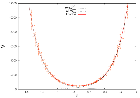
Figure 1: This plot shows the expectation values of the volume observable plotted against ‘time’ $\phi$ in loop quantum cosmology and the Wheeler-DeWitt theory. In loop quantum cosmology, the quantum evolution results in a bounce. In contrast, in the Wheeler-DeWitt theory the expanding and the contracting branches are disjoint and singular. The loop quantum evolution and the Wheeler-DeWitt evolution are in agreement when the spacetime curvature is very small. We also show the trajectory obtained from the effective Hamiltonian constraint in loop quantum cosmology. As can be seen, the latter provides an excellent approximation to the underlying quantum dynamics.

In loop quantum cosmology, we find that the state does not encounter the big bang. Rather, it bounces at a certain volume determined by the field momentum $p_{\phi}$, a constant of motion, on which the initial state is peaked. It turns out that if the state is sharply peaked then irrespective of the choice of $p_{\phi}$, the volume (or the scale factor) of the universe bounces when the energy density of the field reaches a value $\rho_{\rm{max}}\approx 0.41\rho_{\rm{Pl}}$ (Ashtekar et al., 2006c). As we can see from Fig. 1, at large values of volume the evolution in loop quantum cosmology and the Wheeler-DeWitt theory are in excellent agreement. It is only in the small neighborhood of the bounce that there are significant departures between the two theories occur. The quantum gravitational effects in loop quantum cosmology bridge the two singular trajectories in the classical theory. In Fig. 1, we also show a curve which corresponds to a trajectory derived from an effective Hamiltonian constraint in loop quantum cosmology (discussed in the next section), which turns out to be in excellent agreement with the quantum theory at all the scales.

At this point it is natural to ask whether the results of quantum bounce are robust. This question has been answered in several ways. It turns out that the model we studied here can be solved exactly in the $b$ representation (Ashtekar, Corichi, & Singh, 2008). One can then compute the expectation values of volume observable and energy density without resorting to the numerical simulations. It turns out that for all the states in the physical Hilbert space, the expectation values of volume have a non-zero minima, and those of the energy density have a supremum equal to $0.41\rho_{\rm{Pl}}$. Thus, the results of the exactly soluble model are in complete agreement with the numerical simulations. Further, the quantum probability for the bounce to occur for generic states turns out to be unity (Craig & Singh, 2013). Another robustness check comes from rigorous numerical tests (Singh, 2012; Brizuela et al., 2012), including numerical simulations with states which may not be sharply peaked. Recent numerical studies confirm that the quantum bounce occurs for various types of states including those which may have very large quantum fluctuations and non-Gaussian properties (Diener et al., 2014a, b). In fact, the profile of the state is almost preserved and relative fluctuations are tightly constrained across the bounce, in agreement with the analytical results from the exactly soluble model (Corichi & Singh, 2008a; Kaminski & Pawlowski, 2010b; Corichi & Montoya, 2011).

One of the important issues in a quantization is that of ambiguities. Are different consistent loop quantizations of FLRW model possible? Is it possible that the quantum Hamiltonian constraint be a uniform discrete equation in a geometric variable such as area rather than volume? It is interesting to note that by carefully considering mathematical consistency of such alternatives, and demanding that the resulting theory should lead to physics independent of the underlying fiducial structure, one is uniquely led to the loop quantization which is discussed above (Corichi & Singh, 2008b). Similar conclusions have been reached for the Bianchi and Kantowski-Sachs spacetimes (Corichi & Singh, 2009; Singh & Wilson-Ewing, 2014; Joe & Singh, 2014).

4 Effective spacetime description of the isotropic loop quantum cosmology and the generic resolution of singularities

In the previous section, we found that the quantization of the Hamiltonian constraint in loop quantum cosmology results in a quantum difference equation with uniform steps in volume. We also discussed that when gravitational field becomes weak, the quantum difference equation leads to the continuum general relativistic description. An interesting question is whether there exists an effective continuum spacetime description in loop quantum cosmology which reliably captures the underlying physics. If such a description is available, then it can be an important tool to understand the physical implications of loop quantum cosmology. Using the geometrical formulation of the quantum theory (Ashtekar & Schilling, 1999), an effective Hamiltonian constraint in loop quantum cosmology can be obtained for states which are peaked on a classical trajectory at late times, i.e. for universes which grow to a macroscopic sizes (Willis, 2004; Taveras, 2008). The dynamics obtained from the effective Hamiltonian turns out to be in excellent agreement with the underlying quantum dynamics for the sharply peaked states (Ashtekar et al., 2006c; Diener et al., 2014a), which can be seen from the comparison of the quantum evolution and effective trajectory in Fig. 1.

The effective Hamiltonian constraint for the $k=0$ isotropic and homogeneous spacetime is:

$${C}^{\mathrm{(eff)}}_{H}=-\frac{3}{8\pi G\gamma^{2}}\,\frac{\sin^{2}(\lambda b)}{\lambda^{2}}V+\,\rho V\leavevmode\nobreak\ \leavevmode\nobreak\ ,$$ (31)

where $b$ and $V=|p|^{3/2}$ are the conjugate variables satisfying $\{b,V\}=4\pi G\gamma$, and $\lambda=\sqrt{\Delta}$. The vanishing of the Hamiltonian constraint leads to

$$\frac{\sin^{2}(\lambda b)}{\gamma^{2}\lambda^{2}}=\frac{8\pi G}{3}\,\rho\leavevmode\nobreak\ .$$ (32)

Note that the right hand side of the above equation has the same form as that of the classical Friedmann equation, but the left hand side is not the Hubble rate. We can rewrite the above equation in terms of the Hubble rate $H=\dot{a}/a=\dot{V}/3V$, by using the Hamilton’s equation:

$$\dot{V}=-4\pi G\gamma\frac{\partial}{\partial b}{C}^{\mathrm{(eff)}}_{H}=\frac{3}{\gamma}\,\frac{\sin(\lambda b)}{\lambda}\,\cos(\lambda b)\,V\leavevmode\nobreak\ .$$ (33)

Substituting the above equation in eq.(32) and using a trigonometric identity one obtains the modified Friedmann equation in loop quantum cosmology (Ashtekar et al., 2006c; Singh, 2006):

$$H^{2}=\frac{8\pi G}{3}\,\rho\left(1-\frac{\rho}{\rho_{\rm max}}\right)$$ (34)

where $\rho_{\rm max}$ is a constant determined by the quantum discreteness $\lambda$,

$$\rho_{\rm max}=3/(8\pi G\gamma^{2}\lambda^{2})\approx 0.41\rho_{\mathrm{Pl}}\leavevmode\nobreak\ .$$ (35)

One can similarly derive the modified Raychaudhuri equation in loop quantum cosmology by taking the time derivative of eq.(33) and using the Hamilton’s equation $\dot{b}=\{b,{C}^{\mathrm{(eff)}}_{H}\}$, which yields

$$\frac{\ddot{a}}{a}=-\frac{4\pi G}{3}\,\rho\,\left(1-4\frac{\rho}{\rho_{\rm max}}\right)-4\pi G\,P\,\left(1-2\frac{\rho}{\rho_{\rm max}}\right).\leavevmode\nobreak\$$ (36)

Combining the modified Friedmann and Raychaudhuri equations, it is straightforward to see that one recovers the conservation law: $\dot{\rho}+3H\,(\rho+P)=0$.

Let us now analyze some of the main properties of the modified Friedmann and Raychaudhuri equations in loop quantum cosmology. We first note from eq.(34) that the physical solutions have an upper bound on the energy density given by $\rho_{\rm max}$, where the Hubble rate vanishes. This upper bound coincides with the value of bounce density in the numerical simulations with the states which are sharply peaked at late times on the classical trajectory. If the states have very large quantum fluctuations, then there exist departures between the quantum evolution and effective dynamics (Diener et al., 2014a). In that case, the bounce density in the quantum theory is always less than $\rho_{\rm max}$. The modified Friedmann equations in loop quantum cosmology result lead to the classical Friedmann and Raychaudhuri equations when the quantum discreteness $\lambda$ vanishes. In this case, the maximum of the energy density $\rho_{\rm max}$ becomes infinite and the classical singularity is recovered. As mentioned earlier, the non-singular modified Friedmann equations in loop quantum cosmology results in a very rich phenomenology for the background dynamics as well as the cosmological perturbations. For a review of these applications, we refer the reader to Ashtekar & Singh (2011).

Unlike in the classical theory where Hubble rate diverges, such as at the big bang singularity, in loop quantum cosmology the Hubble rate is bounded in the entire evolution. Its maximum value is

$$|H|_{\mathrm{max}}=\left(\frac{1}{\sqrt{3}\,16\pi G\hbar\gamma^{3}}\right)^{1/2}\leavevmode\nobreak\$$ (37)

which is reached at $\rho=\rho_{\rm max}/2$. A consequence of the bounded Hubble rate is that except for the events where the scale factor either vanishes or diverges, the geodesic equations (20) and (21) never break down. But what if the singularity occurs with a vanishing or a diverging scale factor? It turns out that evolution results in either of these possibilities, then the universe in loop quantum cosmology behaves asymptotically as the classical deSitter universe with a rescaled value of the cosmological constant. In the classical theory, geodesics can be extended in the case of the deSitter universe, and thus these points are not problematic for geodesic evolution. Finally, one can rigorously show that the spatially flat isotropic and homogeneous spacetime in effective dynamics of loop quantum cosmology is geodesically complete (Singh, 2009).

It is interesting to note that curvature invariants remain bounded irrespective of the choice of matter. As an example, the Ricci scalar turns out to be The Ricci curvature invariant turns out to be

$$R=8\pi G\rho\,\left(1-3w+2\frac{\rho}{\rho_{\rm max}}\left(1+3w\right)\right).$$ (38)

where $w=P/\rho$. The Ricci scalar, and similarly other curvature invariants, are bounded for all the events where the energy density diverges. Thus, big bang/big crunch, bug rip and big freeze singularities are avoided in loop quantum cosmology. Thus all the strong singularities of the classical FLRW model are absent in loop quantum cosmology (Singh, 2009).

However, the Ricci scalar can diverge when $|w|\rightarrow\infty$, which happens for the type-II singularities. Such ‘soft singularities’ have been shown to exist in loop quantum cosmology (Cailleteau et al., 2008; Singh, 2009; Singh & Vidotto, 2011), but these are harmless because they turn out to be weak singularities in the effective spacetime (as in the classical general relativity). This is straightforward to see from the Królak (22) and Tipler (23) conditions for the existence of strong singularities. As an example, the integrand in Królak and Tipler’s conditions for the null geodesics can be written as

$$R_{ij}u^{i}u^{j}=8\pi G(\rho+P)\frac{\chi^{2}}{a^{2}}\left(1-2\frac{\rho}{\rho_{\rm max}}\right)$$ (39)

which yields the finite result for the integrals in (22) and (23) for type-II singularities. Thus, one finds that the strong singularities are completely avoided in the effective spacetime description of loop quantum cosmology for the spatially flat, isotropic and homogeneous model and only weak singularities can exist. The geodesic evolution never break down for an arbitrary choice of matter. These results are in a striking contrast to the classical FLRW model where unless the universe is deSitter, in general the spacetime is geodesically incomplete and strong singularities exist either in the past or the future evolution.

The robustness of the results of the spatially flat isotropic model has been studied for the $k=\pm 1$ models using a phenomenological equation of state allowing all the types of singularities (Singh & Vidotto, 2011). This analysis confirms that along with the big bang/big crunch, all type-I and type-III singularities are resolved generically. As in the $k=0$ model, quantum gravitational effects ignore the harmless weak singularities. These results have also been generalized to include the anisotropies which we discuss in the following section.

5 Generic resolution of singularities in presence of anisotropies

So far we have focused our discussion only on the isotropic models where we demonstrated the resolution of singularities for arbitrary matter in the effective spacetime description of loop quantum cosmology. We now briefly discuss the way these results generalize to the inclusion of anisotropies in the spacetime. For this we consider the Bianchi-I spacetime which has a spacetime metric:

$$ds^{2}=-\,dt^{2}+a_{1}^{2}\,dx^{2}+a_{2}^{2}dy^{2}+a_{3}^{2}dz^{2}\leavevmode\nobreak\ .$$ (40)

As in the homogeneous isotropic model, in the Bianchi-I spacetime the Ashtekar variables can be expressed in terms of symmetry reduced connections and triads: $c_{i}$ and triads $p_{i}$, which satisfy $\{c_{i},p_{j}\}=8\pi G\gamma\delta_{ij}$. The triads are kinematically related to the scale factors as,

$$|p_{1}|=a_{2}a_{3},\leavevmode\nobreak\ \leavevmode\nobreak\ \leavevmode\nobreak\ |p_{2}|=a_{1}a_{3},\leavevmode\nobreak\ \leavevmode\nobreak\ \leavevmode\nobreak\ |p_{3}|=a_{3}a_{1}\leavevmode\nobreak\ .$$ (41)

Due to homogeneity, the diffeomorphism constraint is satisfied and one is left only with the Hamiltonian constraint, which in terms of $c_{i}$ and $p_{i}$ is:

$${C}^{\mathrm{(cl)}}_{H}=-\frac{1}{8\pi G\gamma^{2}V}{(c_{1}p_{1}\,c_{2}p_{2}+c_{3}p_{3}\,c_{1}p_{1}+c_{2}p_{2}\,c_{3}p_{3})}+\rho V\leavevmode\nobreak\ ,$$ (42)

where $\rho$ denotes the energy density of the matter which is assumed to be of the vanishing anisotropic stress, i.e. it satisfies $\rho(p_{1},p_{2},p_{3})=\rho(p_{1}p_{2}p_{3})$. As in the case of the isotropic model, we can use the Hamilton’s equations, along with the Hamiltonian constraint, to obtain the dynamical equations. One of these equations is the generalized Friedmann equation,

$$H^{2}=\frac{8\pi G}{3}\rho+\sigma^{2}\leavevmode\nobreak\$$ (43)

where $H$ denotes the mean Hubble rate: $H=(H_{1}+H_{2}+H_{3})/3=\dot{V}/3V$, and $\sigma^{2}$ is the shear scalar:

$$\sigma^{2}=\frac{1}{3}\left((H_{1}-H_{2})^{2}+(H_{2}-H_{3})^{2}+(H_{3}-H_{1})^{2}\right)\leavevmode\nobreak\ .$$ (44)

In the classical theory, $\sigma^{2}\propto a^{-6}$. An important implication of this behavior is that unless the equation of state of matter $w$ is greater than or equal to unity, the anisotropies dominate near the singularities. As discussed earlier, the big bang/big crunch singularities can have various structures. These are: a barrel, where one of the scale factor takes a finite values and the other two scale factors vanish; a cigar, where one of the scale factors diverges, and the other two vanish; a pancake, where one of the scale factors vanish and the other two take a finite value; and a point, where all the scale factors vanish. The point like singularity is the isotropic singularity. At these singularities, the directional Hubble rates $H_{i}$, $\rho$ and $\sigma^{2}$ diverge and the geodesic evolution breaks down. This can be seen from analyzing the following geodesic equations in the Bianchi-I spacetime:

$$x^{\prime\prime}=-2x^{\prime}t^{\prime}H_{1},\leavevmode\nobreak\ \leavevmode\nobreak\ y^{\prime\prime}=-2y^{\prime}t^{\prime}H_{2},\leavevmode\nobreak\ \leavevmode\nobreak\ z^{\prime\prime}=-2z^{\prime}t^{\prime}H_{3},\leavevmode\nobreak\ \leavevmode\nobreak\ t^{\prime\prime}=-a_{1}^{2}H_{1}\,x^{\prime 2}-a_{2}^{2}H_{2}\,y^{\prime 2}-a_{3}^{2}H_{3}\,z^{\prime 2}$$ (45)

and

$$x^{\prime}=\frac{k_{x}}{a_{1}^{2}},\leavevmode\nobreak\ \leavevmode\nobreak\ \leavevmode\nobreak\ y^{\prime}=\frac{k_{y}}{a_{2}^{2}},\leavevmode\nobreak\ \leavevmode\nobreak\ \leavevmode\nobreak\ z^{\prime}=\frac{k_{z}}{a_{3}^{2}},\leavevmode\nobreak\ \leavevmode\nobreak\ \leavevmode\nobreak\ t^{\prime}=\left(\frac{k_{x}^{2}}{a_{1}^{2}}+\frac{k_{y}^{2}}{a_{2}^{2}}+\frac{k_{z}^{2}}{a_{3}^{2}}\right)^{1/2}\leavevmode\nobreak\ ,$$ (46)

where $k_{i}$ are constants. From the above equations we find that geodesics break down when any of the scale factors vanishes or the directional Hubble rate diverges. At these events, the curvature invariants blow up. An example of the curvature invariant is the Ricci scalar, whose expression turns out to be

$$R=2\left(H_{1}H_{2}+H_{2}H_{3}+H_{3}H_{1}+\sum_{i=1}^{3}\frac{\ddot{a}_{i}}{a_{i}}\right)\leavevmode\nobreak\ .$$ (47)

We can see that at the big bang/big crunch singularities where the directional Hubble rates and $\ddot{a}_{i}/a_{i}$ diverge, the Ricci scalar becomes infinite. The same is the fate of the other curvature invariants, such as the Kretschmann and the square of the Weyl curvature. These curvature invariant diverging events are strong curvature singularities. Note that for the anisotropic spacetimes, the Tipler and Królak’s conditions also involve integrals over the Weyl curvature components, which should be finite for the singularity to be weak.

Let us now discuss the fate of the singularities in the effective spacetime description of loop quantum cosmology. The loop quantization of the Bianchi-I model has been rigorously performed by Ashtekar & Wilson-Ewing (2009a). Following the strategy for the quantization of the isotropic spacetimes in loop quantum cosmology, the resulting quantum Hamiltonian constraint is a difference operator which turns out to be non-singular. As in the case of the isotropic model, the quantum Hamiltonian constraint in the Bianchi-I model leads to an effective Hamiltonian given by (Chiou & Vandersloot, 2007),

$$C_{H}^{(\rm{eff})}=-\leavevmode\nobreak\ \frac{1}{8\pi G\gamma^{2}V}\left(\frac{\sin(\bar{\mu}_{1}c_{1})}{\bar{\mu}_{1}}\frac{\sin(\bar{\mu}_{2}c_{2})}{\bar{\mu}_{2}}p_{1}p_{2}+\mathrm{cyclic}\leavevmode\nobreak\ \leavevmode\nobreak\ \mathrm{terms}\right)\leavevmode\nobreak\ \leavevmode\nobreak\ +\leavevmode\nobreak\ \leavevmode\nobreak\ \rho V\\$$ (48)

where $\bar{\mu}_{i}$ are:

$$\bar{\mu}_{1}=\lambda\sqrt{\frac{p_{1}}{p_{2}p_{3}}},\leavevmode\nobreak\ \leavevmode\nobreak\ \leavevmode\nobreak\ \bar{\mu}_{2}=\lambda\sqrt{\frac{p_{2}}{p_{1}p_{3}}},\leavevmode\nobreak\ \leavevmode\nobreak\ \leavevmode\nobreak\ \mathrm{and}\leavevmode\nobreak\ \bar{\mu}_{3}=\lambda\sqrt{\frac{p_{3}}{p_{1}p_{2}}}\leavevmode\nobreak\ ,$$ (49)

and the orientation of the triads is chosen to be positive without any loss of generality. The quantum discreteness is captured by $\lambda$, whose square is the minimum area, $\Delta=4\sqrt{3}\pi\gamma l_{\rm Pl}^{2}$, to which loops are shrunk while computing holonomies in loop quantum cosmology. An immediate consequence of the quantum discreteness is the boundedness of the energy density which follows from the vanishing of the Hamiltonian constraint

$$\rho=\frac{1}{8\pi G\gamma^{2}\lambda^{2}}\left(\sin{(\bar{\mu}_{1}c_{1})}\sin{(\bar{\mu}_{2}c_{2})}+\mbox{cyclic terms}\right)\leq\frac{3}{8\pi G\gamma^{2}\lambda^{2}}\approx 0.41\rho_{\rm Pl}$$ (50)

Therefore, in contrast to the classical Bianchi-I model, the energy density can never diverge in the loop quantized Bianchi-I spacetime, and interestingly, the value of the maximum energy density turns out to be the same as in the isotropic model.

Using Hamilton’s equations we can compute the time derivatives of the triads and obtain the expressions for the directional Hubble rates. These turn out to be universally bounded, and so is the mean Hubble rate which has a maximum equal to the maximum Hubble rate in the isotropic model (37):

$$H_{\mathrm{(max)}}=\frac{1}{2\gamma\lambda}\leavevmode\nobreak\ .$$ (51)

From the directional Hubble rates, it is straightforward to find the anisotropic shear scalar:

$$\sigma^{2} = \frac{1}{3\gamma^{2}\lambda^{2}}\Bigg{[}(\cos{(\bar{\mu}_{2}c_{2})}(\sin{(\bar{\mu}_{1}c_{1})}+\sin{(\bar{\mu}_{3}c_{3})})-\cos{(\bar{\mu}_{1}c_{1})}(\sin{(\bar{\mu}_{2}c_{2})}+\sin{(\bar{\mu}_{3}c_{3})}))^{2}$$ (52)

$$+\leavevmode\nobreak\ \mbox{\leavevmode\nobreak\ cyclic terms}\leavevmode\nobreak\ \Bigg{]}\leavevmode\nobreak\ ,$$

which is bounded above by

$${\sigma^{2}}_{\rm max}=\frac{10.125}{3\gamma^{2}\lambda^{2}}.$$ (53)

Thus, the underlying quantum geometric effects incorporated via the minimum area eigenvalue $\lambda^{2}$, bind the mean Hubble rate and the shear scalar in Bianchi-I loop quantum cosmology (Corichi & Singh, 2009; Singh, 2012). If $\lambda$ vanishes, the discrete quantum geometry is replaced by the classical differential geometry, and the magnitude of the above physical quantities have no upper bound. As we discuss below, the boundedness of the mean Hubble rate and the shear scalar has important consequences for the fate of the geodesics and the possibility of the existence of strong singularities in the effective spacetime of Bianchi-I model in loop quantum cosmology.

Note that as we discussed in the case of the isotropic model, even though the energy density, mean Hubble rate and the shear scalar are bounded, the curvature invariants can still diverge for certain choices of equation of states. Analysis of the curvature invariants shows that they are generally bounded but potential divergences can arise if there exists a physical solution for which at a finite value of $\rho,\theta$ and $\sigma^{2}$, pressure diverges and/or the mean volume vanishes (Singh, 2012). None of the known singularities in general relativity satisfy these conditions. Hence, in loop quantum cosmology all of the classical events where curvature invariants diverge are avoided. Does the existence of these potential curvature invariant divergences signal a strong singularity? The answer is tied to whether the divergence occurs due to pressure becoming infinite or the vanishing of one or more scale factors. If the curvature invariants become infinite because of the divergence in the pressure then the event is a weak singularity. However, if the curvature invariants diverge because one of the scale factors vanishes, then the above potential event is a strong singularity. It is important to emphasize that the latter events must occur at a finite value of energy density, mean Hubble rate and the shear scalar. In general relativity, there are no known singularities which satisfy these conditions in the Bianchi-I model, and existence of these events is only a potential mathematical possibility.

Finally, let us discuss the geodesic evolution in the effective spacetime of Bianchi-I model in loop quantum cosmology. Geodesic equations (45) and (46) break down when any of the directional Hubble rates diverge and/or the scale factors $a_{i}$ vanishes. In the classical theory, at the big bang/big crunch singularity at least one of the scale factors always vanish, and one the directional Hubble rate diverges. For the other strong singularities which are of big rip and big freeze type, the scale factors remain finite, however the directional Hubble rates diverge. Thus geodesic evolution in classical Bianchi-I model breaks down at these singularities. In contrast, in loop quantum cosmology all the classical singularities accompanied by a divergence in the directional Hubble rates and the vanishing of the directional scale factors are forbidden, because the former are universally bound by $H_{i\leavevmode\nobreak\ \rm{max}}=3/(2\gamma\lambda)$. The fate of the geodesics for the mathematically possible cases where curvature invariants may diverge in loop quantum cosmology depends on the behavior of the directional scale factors. If the curvature invariants diverge when one of the scale factors vanish at a finite energy density, mean Hubble rate and the shear scalar, then the geodesic equations will break down. However, if the curvature invariants diverge because the pressure becomes infinite, such as in the analog of sudden singularities in the Bianchi-I model, then the geodesics can be extended beyond such events (Singh, 2012). We expect similar results to hold in more general spacetimes, such as the Gowdy models where the above results on boundedness of curvature invariants have already been extended (Tarrío et al., 2013).

6 Summary

The existence of strong singularities in classical spacetimes, signals that a more complete description of the universe will include features of quantum properties of spacetime. These properties which will capture the quantum geometric nature of spacetime are expected to provide insights to many fundamental questions concerning the birth of our universe, the emergence of classical spacetime and the resolution of singularities. In this manuscript, we gave an overview of some of the developments in the framework of loop quantum cosmology, where one uses the techniques of loop quantum gravity to quantize cosmological spacetimes. Attempts to quantize cosmological models date back to the Wheeler-DeWitt theory, however, unlike Wheeler-DeWitt quantum cosmology where resolution of singularities was generally absent, and if present, required very special boundary conditions, in loop quantum cosmology, resolution of big bang singularity has been found to be a robust feature of all the loop quantized spacetimes. As an example, if one considers a sharply peaked state at late times on a classical trajectory in a loop quantized spatially flat homogeneous and isotropic spacetime sourced with a massless scalar field, then such a state follows the classical trajectory in the backward evolution for a very long time, all the way close to the Planck scale, but then bounces to a pre-bounce branch without encountering the big bang singularity (Ashtekar et al., 2006a, b, c). The existence of bounce has been demonstrated to be a robust feature of various spacetimes in loop quantum cosmology. Investigations of the anisotropic models reveal that the evolution is non-singular, and indicate the existence of bounce at the quantum level. These results also extend to the Gowdy models which have infinite degrees of freedom. The underlying loop quantum dynamics can be accurately captured by a continuum non-classical effective description which mimics the quantum evolution very accurately even at the bounce.

The existence of bounce in loop quantum cosmology is a direct ramification of the underlying quantum geometry. The discreteness in geometry bounds the energy density, Hubble rate and anisotropic shear, leading to finite curvature invariants throughout the evolution for all the types of matter with an equation of state which lead to a divergence in the energy density in the classical theory. All of the matter models fall in to this category, except the one with an exotic equation of state, allowing a divergence in pressure at a finite energy density. However, the divergence in curvature invariants does not signal a genuine singularity. Using effective spacetime description, one finds that the events where the curvature invariants diverge in the classical theory, are either completely eliminated in loop quantum cosmology or tun out to be weak singularities (Singh, 2009, 2012). These singularities are harmless because detectors with sufficient strength can propagate across them. Analysis of the geodesic equations signals that the effective spacetime in the spatially flat isotropic model is geodesically complete. For the Bianchi-I model, geodesic evolution does not break down for geodesically inextendible events in the classical theory. Investigations on the behavior of geometric scalars in other Bianchi models (Gupt & Singh, 2012; Singh & Wilson-Ewing, 2014), linearly polarized hybrid Gowdy spacetimes (Tarrío et al., 2013) and Kantowski-Sachs spacetime (Joe & Singh, 2014) indicates that these results may hold in a more general setting.

Thus, in contrast to the classical theory where singularities are a generic feature, there is a growing evidence in loop quantum cosmology that singularities may be absent. An important question in quantum cosmology is whether the results obtained in the homogeneous spacetimes can be trusted in a more general setting. As far as the issue of singularity resolution is concerned, there is a strong evidence from the numerical studies (Berger, 2002; Garfinkle, 2007) of the Belinskii-Khalatnikov-Lifshitz conjecture (Belinskii et al., 1970), that near the singularities the structure of the spacetime is not determined by the spatial derivatives, but by the time derivatives, and the approach to the singularity can be described via homogeneous cosmological models. Thus one can expect that singularity resolution in homogeneous models would capture some aspects of the singularity resolution in more general spacetimes. Recent work in relating the loop quantization of spatially flat isotropic and homogeneous spacetime to that of the Bianchi-I model, also provides useful insights on the role of symmetry reduction (Ashtekar & Wilson-Ewing, 2009a). These results provide evidence that quantization of homogeneous models may reliably capture the nature of quantum spacetime in general near the classical singularities, and to some extent alleviate the concerns about the role of symmetries. One can hope that future work in this direction will keep providing important insights on the fundamental issues both in general relativity and quantum gravity. In particular, one hopes that future investigations on the lines discussed in this manuscript may reveal some important clues to a non-singularity theorem in quantum gravity.

References

- Agullo, Ashtekar & Nelson (2013a) Agullo I., Ashtekar A., Nelson W., 2013a, PhRvD, 87, 043507
- Agullo, Ashtekar & Nelson (2013b) Agullo I., Ashtekar A., Nelson W., 2013b, CQGra., 30, 085014
- Ashtekar (1986) Ashtekar A., 1986, PhRvL, 57, 2244
- Ashtekar & Bojowald (2006) Ashtekar A., Bojowald M., 2006, CQGra, 23, 391
- Ashtekar, Bojowald & Lewandowski (2003) Ashtekar A., Bojowald M., Lewandowski J., 2003, Adv. Theor. Math. Phys., 7, 233
- Ashtekar, Corichi, & Singh (2008) Ashtekar A., Corichi A., Singh P., 2008, PhRvD, 77, 024046
- Ashtekar & Lewandowski (2004) Ashtekar A., Lewandowski J., 2004, CQGra, 21, 53
- Ashtekar et al. (2006a) Ashtekar A., Pawlowski T., Singh P., 2006a, PhRvL, 96, 141301
- Ashtekar et al. (2006b) Ashtekar A., Pawlowski T., Singh P., 2006b, PhRvD, 74, 084003
- Ashtekar et al. (2006c) Ashtekar A., Pawlowski T., Singh P., 2006c, PhRvD, 73, 124038
- Ashtekar et al. (2014) Ashtekar A., Pawlowski T., Singh P., 2014, To appear
- Ashtekar et al. (2007) Ashtekar A., Pawlowski T., Singh P., Vandersloot K., 2007, PhRvD, 75, 024035
- Ashtekar & Schilling (1999) Ashtekar A., Schilling T. A., 1999, On Einstein’s Path, essays in honor of Engelbert Schucking, Ed. Alex Harvey, Springer-Verlag, p 23
- Ashtekar & Singh (2011) Ashtekar A., Singh P., 2011, CQGra, 28, 213001
- Ashtekar & Sloan (2011) Ashtekar A., Sloan D., 2011, GReGr, 43, 3619
- Ashtekar & Sloan (2010) Ashtekar A., Sloan D., 2010, PhLB, 694, 108
- Ashtekar & Wilson-Ewing (2009a) Ashtekar A., Wilson-Ewing E., 2009a, PhRvD, 79, 083535
- Ashtekar & Wilson-Ewing (2009b) Ashtekar A., Wilson-Ewing E., 2009b, PhRvD, 80, 123532
- Barrau et al. (2014) Barrau A., Cailleteau T., Grain J., Mielczarek J., 2014, CQGra., 31, 053001
- Barrow (2004) Barrow J. D., 2004, CQGra, 21, 5619
- Barrow & Tsagas (2005) Barrow J.D., Tsagas C.G., 2005, CQGra., 22, 1563
- Belinskii et al. (1970) Belinskij V. A., Khalatnikov I. M., Lifshits E. M., 1970, AdPhy, 19, 525
- Bentivegna & Pawlowski (2008) Bentivegna E., Pawlowski T., 2008, PhRvD, 77, 124025
- Berger (2002) Berger B. K., 2002, LRR, 5, 1
- Brizuela et al. (2012) Brizuela D., Cartin D., Khanna G., 2012, SIGMA, 8, 1
- Brizuela et al. (2010) Brizuela D., Mena Marugán G. A., Pawlowski T., 2010, CQGra, 27, 052001
- Bojowald (2001) Bojowald M., 2001, PhRvL, 86, 5227
- Borde et al. (2003) Borde A., Guth A. H., Vilenkin A., 2003, PhRvL, 90, 151301
- Bouhmadi-López et al. (2008) Bouhmadi-López M., González-Díaz P. F., Martín-Moruno P., 2008, PhLB, 659, 1
- Cailleteau et al. (2008) Cailleteau T., Cardoso A., Vandersloot K., Wands D., 2008, PhRvL, 101, 251302
- Cailleteau et al. (2009) Cailleteau T., Singh P., Vandersloot K., 2009, PhRvD, 80, 124013
- Caldwell et al. (2003) Caldwell R. R., Kamionkowski M., Weinberg N. N., 2003, PhRvL, 91, 071301
- Chiou (2007) Chiou D.-W., 2007, PhRvD, 75, 024029
- Chiou & Vandersloot (2007) Chiou D.-W., Vandersloot K., 2007, PhRvD, 76, 084015
- Clarke & Królak (1985) Clarke C. J. S., Królak A., 1985, JGP, 2, 127
- Corichi & Karami (2011) Corichi A., Karami A., 2011, PhRvD, 83, 104006
- Corichi & Karami (2014) Corichi A., Karami A., 2014, CQGra., 31, 035008
- Corichi & Montoya (2011) Corichi A., Montoya E., 2011, PhRvD 84, 044021
- Corichi & Singh (2008a) Corichi A., Singh P., 2008a, PhRvL, 100, 161302
- Corichi & Singh (2008b) Corichi A., Singh P., 2008b, PhRvD, 78, 024034
- Corichi & Singh (2009) Corichi A., Singh, P., 2009, PhRvD, 80, 044024
- Corichi & Sloan (2013) Corichi A., Sloan D, 2014, CQGra. 31, 062001
- Craig & Singh (2010) Craig D. A., Singh P., 2010, PhRvD, 82, 123526
- Craig & Singh (2013) Craig D. A., Singh P., 2013, CQGra, 30, 205008
- de Risi, Maartens & Singh (2007) de Risi G., Maartens R., Singh P., 2007, PhRvD, 76, 103531
- Diener et al. (2014a) Diener P., Gupt B., Singh P., 2014, CQGra, 31, 105015
- Diener et al. (2014b) Diener P., Gupt B., Megevand M., Singh P., 2014, CQGra, 31, 165006
- Diener et al. (2014c) Diener P., Gupt B., Megevand M., Singh P., 2014, To appear
- Doroshkevich (1965) Doroshkevich A. G., 1965, Ap, 1, 138
- Ellis (1967) Ellis G. F. R., 1967, JMP, 8, 1171
- Ellis & MacCallum (1969) Ellis G. F. R., MacCallum M. A. H., 1969, CMaPh, 12, 108
- Ellis & Schmidt (1977) Ellis G. F. R., Schmidt B. G., 1977, GReGr, 8, 915
- Fernández-Jambrina & Lazkoz (2004) Fernández-Jambrina L., Lazkoz R., 2004, PhRvD, 70, 121503
- Gambini & Pullin (2011) Gambini R., Pullin J., 2011, A first course in loop quantum gravity, Oxford University Press
- Gambini & Pullin (2008) Gambini R., Pullin J., 2008, PhRvL, 101, 161301
- Gambini & Pullin (2013) Gambini R., Pullin J., 2013, PhRvL, 110, 211301
- Gambini & Pullin (2014) Gambini R., Pullin J., 2014, CQGra, 31, 115003
- Garay et al. (2010) Garay L. J., Martín-Benito M., Mena Marugán G. A., 2010, PhRvD, 82, 044048
- Garfinkle (2007) Garfinkle D., 2007, CQGra. 24, 295
- Garriga, Vilenin & Zhang (2013) Garriga J., Vilenkin A., Zhang J., 2013, JCAP, 11, 55
- Gupt & Singh (2012) Gupt B., Singh P., 2012, PhRvD, 85, 044011
- Gupt & Singh (2013) Gupt B., Singh P., 2013, CQGra, 30, 145013
- Gupt & Singh (2012) Gupt B., Singh P., 2012, PhRvD, 86, 024034
- Gupt & Singh (2014) Gupt B., Singh P., 2014, PhRvD, 89, 063520
- Jacobs (1968) Jacobs K. C., 1968, ApJ, 153, 661
- Joe & Singh (2014) Joe A., Singh P., 2014, arXiv:1407.2428
- Kaminski & Pawlowski (2010a) Kaminski W., Pawlowski T., 2010a, PhRvD, 81, 024014
- Kaminski & Pawlowski (2010b) Kaminski W., Pawlowski T., 2010b, PhRvD, 81, 084027
- Krolak (1986) Krolak A., 1986, CQGra, 3, 267
- Martin-Benito, Garay & Marugan (2008) Martin-Benito M., Garay L. J., Marugan G. A. M., 2008, PhRvD 78, 083516
- Martin-Benito, Marugan, Pawlowski (2009) Martin-Benito M., Mena Marugan G. A., Pawlowski T., 2009, PhRvD, 80, 084038
- Naskar & Ward (2007) Naskar T., Ward J., 2007, PhRvD 76, 063514
- Nojiri et al. (2005) Nojiri S., Odintsov S. D., Tsujikawa S., 2005, PhRvD, 71, 063004
- Pawlowski, Ashtekar (2012) Pawlowski T., Ashtekar A., 2012, PhRvD, 85, 064001
- Pawlowski et al. (2014) Pawlowski T., Pierini R., Wilson-Ewing E., 2014, arXiv:1404.4036
- Ranken & Singh (2012) Ranken E., Singh P., 2012, PhRvD 85, 104002
- Rovelli (2004) Rovelli C., 2004, Quantum Gravity, Cambridge University Press
- Samart & Gumjudpai (2007) Samart D., Gumjudpai B., 2007, PhRvD, 76, 043514
- Sami et al. (2006) Sami M., Singh P., Tsujikawa S., 2006, PhRvD, 74, 043514
- Shtanov & Sahni (2003) Shtanov Y., Sahni V., 2003, PhLB, 557, 1
- Singh (2006) Singh P., 2006, PhRvD, 73, 063508
- Singh (2009) Singh P., 2009, CQGra, 26, 125005
- Singh (2012) Singh P., 2012, PhRvD, 85, 104011
- Singh (2012) Singh P., 2012, CQGra, 29, 244002
- Singh, Sami & Dadhich (2003) Singh P., Sami M., Dadhich N., 2003, Phys. Rev. D 68, 023522
- Singh, Vandersloot & Vereshchagin (2006) Singh P., Vandersloot K., Vereshchagin G. V., 2006, PhRvD 74, 043510
- Singh & Vidotto (2011) Singh P., Vidotto F., 2011, PhRvD, 83, 064027
- Singh & Wilson-Ewing (2014) Singh P., Wilson-Ewing E., 2014, CQGra, 31, 035010
- Szulc et al. (2007) Szulc Ł., Kaminski W., Lewandowski J., 2007, CQGra, 24, 2621
- Szulc (2007) Szulc Ł., 2007, CQGra, 24, 6191
- Tarrío et al. (2013) Tarrío P., Fernández-Méndez M., Mena Marugán G. A., 2013, PhRvD, 88, 084050
- Taveras (2008) Taveras V., 2008, PhRvD, 78, 064072
- Thiemann (2007) Thiemann, T. 2007, Modern Canonical Quantum General Relativity, Cambridge University Press
- Thorne (1967) Thorne K. S., 1967, ApJ, 148, 51
- Tipler (1977) Tipler F. J., 1977, PhLA, 64, 8
- Vandersloot (2007) Vandersloot K., 2007, PhRvD, 75, 023523
- Cattoën & Visser (2005) Cattoën C., Visser M., 2005, CQGra, 22, 4913
- Willis (2004) Willis J. L., 2004, PhD Thesis, Pennsylvania State University
- Wilson-Ewing (2010) Wilson-Ewing E., 2010, PhRvD, 82, 043508