An Introduction to Twisted Particle Filters and Parameter Estimation in Non-linear State-space Models

Juha Ala-Luhtala, Nick Whiteley, Kari Heine and Robert Piché J. Ala-Luhtala is with the Department of Mathematics, Tampere University of Technology, PO Box 553, 33101, Tampere, Finland, e-mail: juha.ala-luhtala@tut.fi.N. Whiteley is with the School of Mathematics, University of Bristol, University Walk, Bristol, BS8 1TW, UK, e-mail: nick.whiteley@bristol.ac.ukK. Heine is with the Department of Statistical Science, University College London, Gower Street, London, WC1E 6BT, UK, e-mail: k.heine@ucl.ac.ukR. Piché is with the Department of Automation Science and Engineering, Tampere University of Technology, e-mail: robert.piche@tut.fi.
Abstract

Twisted particle filters are a class of sequential Monte Carlo methods recently introduced by Whiteley and Lee [1] to improve the efficiency of marginal likelihood estimation in state-space models. The purpose of this article is to extend the twisted particle filtering methodology, establish accessible theoretical results which convey its rationale, and provide a demonstration of its practical performance within particle Markov chain Monte Carlo for estimating static model parameters. We derive twisted particle filters that incorporate systematic or multinomial resampling and information from historical particle states, and a transparent proof which identifies the optimal algorithm for marginal likelihood estimation. We demonstrate how to approximate the optimal algorithm for nonlinear state-space models with Gaussian noise and we apply such approximations to two examples: a range and bearing tracking problem and an indoor positioning problem with Bluetooth signal strength measurements. We demonstrate improvements over standard algorithms in terms of variance of marginal likelihood estimates and Markov chain autocorrelation for given CPU time, and improved tracking performance using estimated parameters.

Index Terms:
Particle filter, sequential Monte Carlo, particle MCMC, Gaussian state-space model, parameter estimation.

I Introduction

State-space models are applied to a wide variety of signal processing problems, especially in positioning, tracking and navigation [2, 3, 4]. These models need to be calibrated by inferring unknown parameters from data. There are a variety of approaches to this inference problem, such as maximum likelihood (ML) or maximum a posteriori (MAP) estimation using the Expectation Maximization algorithm or Laplace approximations, Gaussian filtering based approximations, and state augmentation techniques [5, 6, 3]. In this paper we consider a Bayesian approach, which has the advantage of allowing prior information about parameters to be imparted, and a variety of estimates and measures of uncertainty to be reported based on the posterior distribution. By using a Markov chain Monte Carlo (MCMC) algorithm, e.g. Metropolis-Hastings (M-H) (see [7] for an introduction), one can in principle explore the entire posterior, but in practice the design of efficient MCMC algorithm can be a challenging task.

A direct application of M-H to a state-space model requires evaluation of the marginal likelihood of data, which is a high-dimensional, analytically intractable integral in many cases of interest. However, this issue can be circumvented through the application of pseudo-marginal MCMC methods [8, 9], which allow MCMC algorithms yielding samples from the desired posterior to be constructed if an unbiased estimator of the marginal likelihood is available. Particle filters [10] (see [4, 3] for overviews in the context of tracking applications) provide such an estimator, and the resulting MCMC scheme is known as a particle Markov chain Monte Carlo (PMCMC) method [11]. Typically the most substantial contribution to the overall cost of a PMCMC algorithm arises from the need to run a particle filter at each iteration of the MCMC sampler, and the performance of the sampler is sensitive to the variability of the marginal likelihood estimate which the particle filter delivers [12]. This motivates the development of particle filters which can provide reliable marginal likelihood estimates at a low computational cost.

In this paper we develop new “twisted particle filtering” methodology, building from ideas recently introduced by [1]. Twisted particle filters are purposefully designed to provide more reliable approximations of marginal likelihoods than standard particle filters, while preserving the lack-of-bias property which permits their use within PMCMC.

Unlike traditional approaches to improving the efficiency of particle filters which modify the proposal distribution on a per-particle basis [13] or employ auxiliary weights for resampling [14], twisted particle filters are derived by applying a form of re-weighting to the particle system as a whole, using a so-called “twisting” function. The role of the twisting function is to incorporate information from the observations, possibly future and past, into the mechanism by which particles are propagated over time. The ability to choose different twisting functions introduces a degree of freedom into the design of the particle algorithm, leading naturally to questions of optimality. In concrete terms, if the twisting function is chosen well, the twisted particle filter can estimate the marginal likelihood with greater accuracy than a standard particle filter, in turn allowing more efficient estimation inference for static parameters in the state-space model.

The investigations of [1] focussed mainly on theoretical analysis of twisted particle filters, studying their asymptotic properties in the regimes where the number of particles tends to infinity and where the length of the time horizon grows, under probabilistic assumptions on the observation sequence and strong regularity conditions on the statistical model.

The objectives of this paper are to present new twisted particle filtering methodology, validate it theoretically, and demonstrate its application and effectiveness within PMCMC for inferring the parameters of state-space models. Our main contributions are as follows.

I-1 Algorithms

We introduce a general formulation of twisted particle filters. The first novel aspect of this formulation beyond that given in [1], is that it allows various resampling methods to be incorporated in twisted particle filters. In particular, we derive a twisted particle filter around the popular systematic resampling method, which is known to reduce variance within the particle filter. The second novel aspect of the new formulation is that it allows for twisting functions which depend on historical particle states, which is an important factor when designing them efficiently in practice. The methodology of [1], which treated only multinomial resampling and twisting functions which depend only on current particle states. The utility of these algorithmic developments is that they allow for more accurate estimation of marginal likelihoods.

I-2 Theory

We provide novel theoretical results which justify the new algorithms and characterize their optimal operation. The first result, Theorem 1, establishes the lack-of-bias property of the marginal likelihood approximation delivered by the new twisted particle filter. The importance of this result is that it justifies the use of the twisted particle filter within PMCMC, whilst allowing for more general structure of the resampling technique and twisting function than in [1].

The second result, Theorem 2, identifies the twisting functions which are optimal for approximating the marginal likelihood for a given finite number of observations. This provides a different perspective to the results of [1], which are asymptotic in nature, considering optimality in terms of minimal variance growth rate in the regime where the length of the data record tends to infinity. Theorem 2 relies on only mild regularity assumptions on the ingredients of the twisted particle filter, whereas the results of [1] assume a particularly strong form of geometric ergodicity of the signal in the hidden Markov model (HMM) and certain uniform upper and lower bounds on the likelihood functions. Moreover, compared to the analyses of [1], the proof of Theorem 2 is less intricate, and gives the reader a more accessible route to understanding how twisted particle filters work.

I-3 Approximation techniques

Informed by Theorem 2, we propose methods to approximate the optimal twisting function for nonlinear Gaussian state-space models, based on ideas of Kalman filtering methodology together with local linearization using historical particle states.

I-4 Applications and numerical results

We provide numerical results in the context of two applications.

The first application is a range and bearing tracking problem. This is a classical nonlinear tracking scenario and serves as a benchmark application of particle filters [15], [2]. The purpose of this example is to compare the performance of twisted particle filters and the corresponding PMCMC algorithms to standard particle filters in a situation where the ground truth for static parameters is available, with simulated data. The twisted particle filters we consider employ linearization techniques to approximate the optimal twisting functions. The results we obtain illustrate that twisted particle filters can more reliably approximate marginal likelihoods for the same or less computational cost than standard particle filters. The benefits of using twisted particle filters within PMCMC are also demonstrated in terms of lower auto-correlation, and consequently more accurate approximation of posterior distributions over static parameters. We also compare tracking performance based on estimated parameter values.

The second application is a more complex indoor positioning problem. In this application a state-space model represents the unknown position of a user over time, observed indirectly and with uncertainty through received signal strength (RSS) measurements. Such data are widely available from many different wireless communication systems including mobile networks and WLAN. They have been proposed for use in location estimation in a variety of novel location-aware applications, such as environmental and structure monitoring, and many military and public safety applications, see [16], [17] and references therein. We work with a real Bluetooth RSS data set. A key task when dealing with RSS measurements is to calibrate the model by estimating unknown parameters which describe attenuation characteristics of the environment in which the user moves, since otherwise one must resort to oversimplified models [17], which exhibit inferior tracking performance.

A variety of approaches to estimating these parameters have been suggested, involving least squares [17] and weighted least squares [18] methods. These techniques provide point estimates of parameter values from a batch of data. Bayesian approaches, e.g., [19], allow additionally for uncertainty associated with estimates to be reported, and incorporate prior distributions to quantify expert knowledge and physical constraints on parameter values. They also naturally handle uncertainty over state variables when inferring parameters through marginalization.

The price to pay for the Bayesian approach is the computational cost of Monte Carlo sampling, and so our numerical investigations largely focus on computational efficiency. We compare the performance of twisted particle filters to more standard particle filters using a variety of proposal and resampling techniques. We demonstrate improved CPU-time efficiency in estimating marginal likelihoods, and we show that this efficiency is carried over to the particle MCMC algorithm, giving performance gains in terms of quality of the resulting MCMC chain compared to PMCMC using a standard particle filter. We also demonstrate favourable tracking performance using parameter estimates obtained from PMCMC.

The structure of the paper is as follows. Section II gives the problem formulation. Section III introduces a PMCMC algorithm and a standard particle filter. Section IV presents the twisted particle filtering methodology and Theorems 1-2, which characterize the lack-of-bias property and optimal twisting functions. Computational complexity is also discussed. Section V introduces methods for approximating the optimal twisting functions in nonlinear state-space models with Gaussian noise. Section VI contains applications and numerical results. Finally, conclusions are presented in Section VII.

II Problem formulation

We first introduce some notation. Uppercase is used to denote random variables (e.g. X,Y,𝑋𝑌X,Y,\ldots) and realized values are denoted with lowercase (e.g. x,y,𝑥𝑦x,y,\ldots). For any sequence (an)n0subscriptsubscript𝑎𝑛𝑛0(a_{n})_{n\geq 0} and sk𝑠𝑘s\leq k we write as:k:=(as,,ak)assignsubscript𝑎:𝑠𝑘subscript𝑎𝑠subscript𝑎𝑘a_{s:k}:=(a_{s},\ldots,a_{k}).

We consider state-space models of the form

X0μ0,θ(),Xksimilar-tosubscript𝑋0subscript𝜇0𝜃subscript𝑋𝑘\displaystyle X_{0}\sim\mu_{0,\theta}(\cdot),\quad X_{k} fk,θ(|Xk1),k1,\displaystyle\sim f_{k,\theta}(\cdot\,|\,X_{k-1}),\quad k\geq 1,
Yksubscript𝑌𝑘\displaystyle Y_{k} gk,θ(|Xk),k0,\displaystyle\sim g_{k,\theta}(\cdot\,|\,X_{k}),\quad k\geq 0, (1)

where Xk𝕏subscript𝑋𝑘𝕏X_{k}\in\mathbb{X} is the state vector, Yk𝕐ksubscript𝑌𝑘subscript𝕐𝑘Y_{k}\in\mathbb{Y}_{k} is the measurement vector, μ0,θ()subscript𝜇0𝜃\mu_{0,\theta}(\cdot) is the initial distribution, fk,θ(|xk1)f_{k,\theta}(\cdot\,|\,x_{k-1}) describes the transitions of the state process and gk,θ(|xk)g_{k,\theta}(\cdot\,|\,x_{k}) is the conditional distribution for the measurement. All the model distributions are assumed to admit probability densities denoted with the same letter as the distribution. The joint density of the state-variables and measurements for k1𝑘1k\geq 1 is given by

pθ(y0:k,x0:k)subscript𝑝𝜃subscript𝑦:0𝑘subscript𝑥:0𝑘\displaystyle p_{\theta}(y_{0:k},x_{0:k}) =μ0,θ(x0)g0,θ(y0|x0)absentsubscript𝜇0𝜃subscript𝑥0subscript𝑔0𝜃conditionalsubscript𝑦0subscript𝑥0\displaystyle=\mu_{0,\theta}(x_{0})g_{0,\theta}(y_{0}\,|\,x_{0})
s=1kfs,θ(xs|xs1)gs,θ(ys|xs).\displaystyle\quad\cdot\prod_{s=1}^{k}f_{s,\theta}(x_{s}\,|\,x_{s-1})g_{s,\theta}(y_{s}\,|\,x_{s}). (2)

The parameter vector θdθ𝜃superscriptsubscript𝑑𝜃\theta\in\mathbb{R}^{d_{\theta}} contains all the unknown parameters of the model.

We are mainly concerned in estimating the unknown parameters θ𝜃\theta using a set of realized measurements y0:tsubscript𝑦:0𝑡y_{0:t}. In the Bayesian framework, the parameters are considered as random variables and estimates are computed using the posterior distribution

p(θ|y0:t)pθ(y0:t)p(θ),proportional-to𝑝conditional𝜃subscript𝑦:0𝑡subscript𝑝𝜃subscript𝑦:0𝑡𝑝𝜃p(\theta\,|\,y_{0:t})\propto p_{\theta}(y_{0:t})p(\theta), (3)

where pθ(y0:t)subscript𝑝𝜃subscript𝑦:0𝑡p_{\theta}(y_{0:t}) is the likelihood and p(θ)𝑝𝜃p(\theta) is the prior.

With the shorthand

πk,θ(dxk):=pθ(dxk|y0:k1),πk,θ(dxk):=pθ(dxk|y0:k),formulae-sequenceassignsuperscriptsubscript𝜋𝑘𝜃𝑑subscript𝑥𝑘subscript𝑝𝜃conditional𝑑subscript𝑥𝑘subscript𝑦:0𝑘1assignsubscript𝜋𝑘𝜃𝑑subscript𝑥𝑘subscript𝑝𝜃conditional𝑑subscript𝑥𝑘subscript𝑦:0𝑘\pi_{k,\theta}^{-}(dx_{k}):=p_{\theta}(dx_{k}\,|\,y_{0:k-1}),\;\;\pi_{k,\theta}(dx_{k}):=p_{\theta}(dx_{k}\,|\,y_{0:k}),

the likelihood term can be evaluated recursively, for k1𝑘1k\geq 1,

pθ(y0:k)subscript𝑝𝜃subscript𝑦:0𝑘\displaystyle p_{\theta}(y_{0:k}) =pθ(y0:k1)𝕏gk,θ(yk|xk)πk,θ(dxk),absentsubscript𝑝𝜃subscript𝑦:0𝑘1subscript𝕏subscript𝑔𝑘𝜃conditionalsubscript𝑦𝑘subscript𝑥𝑘superscriptsubscript𝜋𝑘𝜃𝑑subscript𝑥𝑘\displaystyle=p_{\theta}(y_{0:k-1})\int_{\mathbb{X}}g_{k,\theta}(y_{k}\,|\,x_{k})\pi_{k,\theta}^{-}(dx_{k}), (4)

pθ(y0)=𝕏g0,θ(y0|x0)μ0,θ(dx0)subscript𝑝𝜃subscript𝑦0subscript𝕏subscript𝑔0𝜃conditionalsubscript𝑦0subscript𝑥0subscript𝜇0𝜃𝑑subscript𝑥0p_{\theta}(y_{0})=\int_{\mathbb{X}}g_{0,\theta}(y_{0}\,|\,x_{0})\mu_{0,\theta}(dx_{0}), and

πk,θ(xk)=𝕏fk,θ(xk|xk1)πk1,θ(dxk1),k1,formulae-sequencesuperscriptsubscript𝜋𝑘𝜃subscript𝑥𝑘subscript𝕏subscript𝑓𝑘𝜃conditionalsubscript𝑥𝑘subscript𝑥𝑘1subscript𝜋𝑘1𝜃𝑑subscript𝑥𝑘1𝑘1\pi_{k,\theta}^{-}(x_{k})=\int_{\mathbb{X}}f_{k,\theta}(x_{k}\,|\,x_{k-1})\pi_{k-1,\theta}(dx_{k-1}),\;k\geq 1, (5)
πk,θ(xk){g0,θ(y0|x0)μ0,θ(x0),k=0,gk,θ(yk|xk)πk,θ(xk),k1.proportional-tosubscript𝜋𝑘𝜃subscript𝑥𝑘casessubscript𝑔0𝜃conditionalsubscript𝑦0subscript𝑥0subscript𝜇0𝜃subscript𝑥0𝑘0subscript𝑔𝑘𝜃conditionalsubscript𝑦𝑘subscript𝑥𝑘superscriptsubscript𝜋𝑘𝜃subscript𝑥𝑘𝑘1\pi_{k,\theta}(x_{k})\propto\left\{\begin{array}[]{cc}g_{0,\theta}(y_{0}\,|\,x_{0})\mu_{0,\theta}(x_{0}),&k=0,\\ g_{k,\theta}(y_{k}\,|\,x_{k})\pi_{k,\theta}^{-}(x_{k}),&k\geq 1.\end{array}\right. (6)

Exact inference using (3) directly is usually intractable, since the likelihood term can be evaluated exactly for only some special models (e.g. linear Gaussian model). We consider particle filtering methods for computing unbiased estimates for the likelihood term. These can then be used as a part of particle MCMC methods that draw samples from the posterior distribution of interest.

III Particle MCMC

In this section we describe methods for drawing samples from the parameter posterior distribution in (3). Algorithms targeting only the parameter posterior are often called marginal algorithms, because samples are drawn only from the marginal posterior p(θ|y0:t)𝑝conditional𝜃subscript𝑦:0𝑡p(\theta\,|\,y_{0:t}) instead of the full posterior p(x0:t,θ|y0:t)𝑝subscript𝑥:0𝑡conditional𝜃subscript𝑦:0𝑡p(x_{0:t},\theta\,|\,y_{0:t}).

MCMC methods generate samples from the target posterior distribution by simulating a Markov chain θ0,θ1,superscript𝜃0superscript𝜃1\theta^{0},\theta^{1},\ldots that has the target posterior distribution as a stationary distribution [7]. One of the best known and general MCMC methods is the Metropolis-Hastings (MH) algorithm, where a new sample θsuperscript𝜃\theta^{*} at step i𝑖i is generated from a proposal distribution κ(|θi1)\kappa(\cdot\,|\,\theta^{i-1}). The generated sample θsuperscript𝜃\theta^{*} is then accepted with probability

min{1,pθ(y0:t)p(θ)pθi1(y0:t)p(θi1)κ(θi1|θ)κ(θ|θi1)}.1subscript𝑝superscript𝜃subscript𝑦:0𝑡𝑝superscript𝜃subscript𝑝superscript𝜃𝑖1subscript𝑦:0𝑡𝑝superscript𝜃𝑖1𝜅conditionalsuperscript𝜃𝑖1superscript𝜃𝜅conditionalsuperscript𝜃superscript𝜃𝑖1\min\left\{1,\frac{p_{\theta^{*}}(y_{0:t})p(\theta^{*})}{p_{\theta^{i-1}}(y_{0:t})p(\theta^{i-1})}\frac{\kappa(\theta^{i-1}\,|\,\theta^{*})}{\kappa(\theta^{*}\,|\,\theta^{i-1})}\right\}. (7)

To compute this acceptance probability, we need to evaluate likelihood terms pθ(y0:t)subscript𝑝𝜃subscript𝑦:0𝑡p_{\theta}(y_{0:t}), but that is not possible for a general nonlinear state-space model. However, if an unbiased estimator for the likelihood is available, it is still possible to construct an MCMC algorithm to sample from the posterior distribution [8, 9]. For state-space models, we can use particle filters as unbiased estimators of the likelihood [11]. A Metropolis-Hastings algorithm using particle filters to estimate the likelihood terms, called particle marginal Metropolis-Hastings (PMMH) [11], is given in Algorithm 1.

1:Sample θ0p(θ)similar-tosuperscript𝜃0𝑝𝜃\theta^{0}\sim p(\theta)
2:Obtain an unbiased estimate Z0superscript𝑍0Z^{0} of pθ0(y0:t)subscript𝑝superscript𝜃0subscript𝑦:0𝑡p_{\theta^{0}}(y_{0:t})
3:for i1𝑖1i\geq 1 do
4:     Sample θκ(|θi1)\theta^{*}\sim\kappa(\cdot\,|\,\theta^{i-1})
5:     Obtain an unbiased estimate Zsuperscript𝑍Z^{*} of pθ(y0:t)subscript𝑝superscript𝜃subscript𝑦:0𝑡p_{\theta^{*}}(y_{0:t})
6:     Set α=min{1,Zp(θ)Zi1p(θi1)κ(θi1|θ)κ(θ|θi1)}𝛼1superscript𝑍𝑝superscript𝜃superscript𝑍𝑖1𝑝superscript𝜃𝑖1𝜅conditionalsuperscript𝜃𝑖1superscript𝜃𝜅conditionalsuperscript𝜃superscript𝜃𝑖1\alpha=\min\left\{1,\dfrac{Z^{*}p(\theta^{*})}{Z^{i-1}p(\theta^{i-1})}\dfrac{\kappa(\theta^{i-1}\,|\,\theta^{*})}{\kappa(\theta^{*}\,|\,\theta^{i-1})}\right\}
7:     Sample U𝑈U from a uniform distribution on [0,1]01[0,1]
8:     if U<α𝑈𝛼U<\alpha then
9:         Set θi=θsuperscript𝜃𝑖superscript𝜃\theta^{i}=\theta^{*} and Zi=Zsuperscript𝑍𝑖superscript𝑍Z^{i}=Z^{*}
10:     else
11:         Set θi=θi1superscript𝜃𝑖superscript𝜃𝑖1\theta^{i}=\theta^{i-1} and Zi=Zi1superscript𝑍𝑖superscript𝑍𝑖1Z^{i}=Z^{i-1}
12:     end if
13:end for
Algorithm 1: Particle marginal Metropolis-Hastings

III-A Particle filtering

We proceed with an account of a standard particle filter. Our notation is in some places a little non-standard, but is chosen deliberately to help with the derivation of twisted particle filters in Section IV. Henceforth, for notational simplicity, we often omit the subscript θ𝜃\theta and implicitly assume that the distributions can depend on the parameters.

We denote the set of n1𝑛1n\geq 1 particles at time k0𝑘0k\geq 0 by ξk=(ξki)i=1nsubscript𝜉𝑘superscriptsubscriptsuperscriptsubscript𝜉𝑘𝑖𝑖1𝑛\xi_{k}=(\xi_{k}^{i})_{i=1}^{n}, with corresponding unnormalized weights Wk=(Wki)i=1nsubscript𝑊𝑘superscriptsubscriptsuperscriptsubscript𝑊𝑘𝑖𝑖1𝑛W_{k}=(W_{k}^{i})_{i=1}^{n}. The filtering distribution is approximated by

πk,θ(dxk)i=1nWkiδξki(dxk)i=1nWki,subscript𝜋𝑘𝜃𝑑subscript𝑥𝑘superscriptsubscript𝑖1𝑛superscriptsubscript𝑊𝑘𝑖subscript𝛿superscriptsubscript𝜉𝑘𝑖𝑑subscript𝑥𝑘superscriptsubscript𝑖1𝑛superscriptsubscript𝑊𝑘𝑖\pi_{k,\theta}(dx_{k})\approx\frac{\sum_{i=1}^{n}W_{k}^{i}\delta_{\xi_{k}^{i}}(dx_{k})}{\sum_{i=1}^{n}W_{k}^{i}}, (8)

where δξki()subscript𝛿superscriptsubscript𝜉𝑘𝑖\delta_{\xi_{k}^{i}}(\cdot) denotes a unit point mass centered at ξkisuperscriptsubscript𝜉𝑘𝑖\xi_{k}^{i}.

In order to describe the sampling mechanism for the particles and understand certain properties of the algorithm it is convenient to also introduce, for each k0𝑘0k\geq 0, the ancestor indicator variables Ak=(Aki)i=1nsubscript𝐴𝑘superscriptsubscriptsuperscriptsubscript𝐴𝑘𝑖𝑖1𝑛A_{k}=(A_{k}^{i})_{i=1}^{n}, where each Akisuperscriptsubscript𝐴𝑘𝑖A_{k}^{i} takes a value in {1,,n}1𝑛\{1,\ldots,n\}. If we also define for each k0𝑘0k\geq 0 and i{1,,n}𝑖1𝑛i\in\{1,\ldots,n\}, (Bk,ji)j=0ksuperscriptsubscriptsuperscriptsubscript𝐵𝑘𝑗𝑖𝑗0𝑘(B_{k,j}^{i})_{j=0}^{k} by letting Bk,ki:=iassignsuperscriptsubscript𝐵𝑘𝑘𝑖𝑖B_{k,k}^{i}:=i and for k>0𝑘0k>0, recursively Bk,j:=AjBk,j+1assignsubscript𝐵𝑘𝑗superscriptsubscript𝐴𝑗subscript𝐵𝑘𝑗1B_{k,j}:=A_{j}^{B_{k,j+1}}, j=k1,,0𝑗𝑘10j=k-1,\ldots,0, then we can write the “ancestral line” of particle ξkisuperscriptsubscript𝜉𝑘𝑖\xi_{k}^{i} as

ki:=(ξki,ξk1Bk,k1i,,ξ0Bk,0i),assignsuperscriptsubscript𝑘𝑖superscriptsubscript𝜉𝑘𝑖superscriptsubscript𝜉𝑘1superscriptsubscript𝐵𝑘𝑘1𝑖superscriptsubscript𝜉0superscriptsubscript𝐵𝑘0𝑖\mathscr{L}_{k}^{i}:=(\xi_{k}^{i},\xi_{k-1}^{B_{k,k-1}^{i}},\ldots,\xi_{0}^{B_{k,0}^{i}}), (9)

which is a 𝕏k+1superscript𝕏𝑘1\mathbb{X}^{k+1}-valued random variable.

1:for 1in1𝑖𝑛1\leq i\leq n do
2:     Sample ξ0iq0()similar-tosuperscriptsubscript𝜉0𝑖subscript𝑞0\xi_{0}^{i}\sim q_{0}(\cdot)
3:     Set W0i=g0(y0|ξ0i)μ0(ξ0i)/q0(ξ0i)subscriptsuperscript𝑊𝑖0subscript𝑔0conditionalsubscript𝑦0superscriptsubscript𝜉0𝑖subscript𝜇0superscriptsubscript𝜉0𝑖subscript𝑞0superscriptsubscript𝜉0𝑖W^{i}_{0}=g_{0}(y_{0}\,|\,\xi_{0}^{i})\mu_{0}(\xi_{0}^{i})/q_{0}(\xi_{0}^{i})
4:end for
5:Set Z0=1ni=1nW0isubscript𝑍01𝑛superscriptsubscript𝑖1𝑛superscriptsubscript𝑊0𝑖Z_{0}=\frac{1}{n}\sum_{i=1}^{n}W_{0}^{i}
6:for 1kt1𝑘𝑡1\leq k\leq t do
7:     Sample Uk1𝒰[0,1]msimilar-tosubscript𝑈𝑘1𝒰superscript01𝑚U_{k-1}\sim\mathcal{U}[0,1]^{m}
8:     Set Ak1=r(Uk1,Wk1)subscript𝐴𝑘1𝑟subscript𝑈𝑘1subscript𝑊𝑘1A_{k-1}=r(U_{k-1},W_{k-1})
9:     for 1in1𝑖𝑛1\leq i\leq n do
10:         Sample ξkiqk(|k1Ak1i)\xi_{k}^{i}\sim q_{k}(\cdot\,|\,\mathscr{L}_{k-1}^{A_{k-1}^{i}})
11:         Set Wki=gk(yk|ξki)fk(ξki|ξk1Ak1i)qk(ξki|k1Ak1i)superscriptsubscript𝑊𝑘𝑖subscript𝑔𝑘conditionalsubscript𝑦𝑘superscriptsubscript𝜉𝑘𝑖subscript𝑓𝑘conditionalsuperscriptsubscript𝜉𝑘𝑖superscriptsubscript𝜉𝑘1superscriptsubscript𝐴𝑘1𝑖subscript𝑞𝑘conditionalsuperscriptsubscript𝜉𝑘𝑖superscriptsubscript𝑘1superscriptsubscript𝐴𝑘1𝑖W_{k}^{i}=\dfrac{g_{k}(y_{k}\,|\,\xi_{k}^{i})f_{k}(\xi_{k}^{i}\,|\,\xi_{k-1}^{A_{k-1}^{i}})}{q_{k}(\xi_{k}^{i}\,|\,\mathscr{L}_{k-1}^{A_{k-1}^{i}})}
12:     end for
13:     Set Zk=Zk11ni=1nWkisubscript𝑍𝑘subscript𝑍𝑘11𝑛superscriptsubscript𝑖1𝑛superscriptsubscript𝑊𝑘𝑖Z_{k}=Z_{k-1}\frac{1}{n}\sum_{i=1}^{n}W_{k}^{i}
14:end for
Algorithm 2: Particle filter

A particle filter is given in Algorithm 2. Here the proposal distributions (qk)k0subscriptsubscript𝑞𝑘𝑘0(q_{k})_{k\geq 0} are assumed to be chosen such that for each k0𝑘0k\geq 0 the weights Wksubscript𝑊𝑘W_{k} are strictly positive and finite. Each qksubscript𝑞𝑘q_{k} may be chosen to depend also on the observations y0:ksubscript𝑦:0𝑘y_{0:k}, but this dependence is suppressed from the notation.

III-B Resampling

Lines 7 and 8 in Algorithm 2 together implement a generic resampling operation. Line 7 generates Uk1=(Uk1i)i=1msubscript𝑈𝑘1superscriptsubscriptsuperscriptsubscript𝑈𝑘1𝑖𝑖1𝑚U_{k-1}=(U_{k-1}^{i})_{i=1}^{m} consisting of m1𝑚1m\geq 1 i.i.d. random variables, each uniformly distributed on [0,1]01[0,1]. Line 8 passes Uk1subscript𝑈𝑘1U_{k-1} and the unnormalized weights Wk1subscript𝑊𝑘1W_{k-1} to a deterministic mapping r:[0,1]m×+n{1,,n}n:𝑟superscript01𝑚superscriptsubscript𝑛superscript1𝑛𝑛r\colon[0,1]^{m}\times\mathbb{R}_{+}^{n}\to\{1,\ldots,n\}^{n}, which returns the ancestor indicator variables Ak1=(Ak1i)i=1nsubscript𝐴𝑘1superscriptsubscriptsuperscriptsubscript𝐴𝑘1𝑖𝑖1𝑛A_{k-1}=(A_{k-1}^{i})_{i=1}^{n}. With ri(Uk1,Wk1)superscript𝑟𝑖subscript𝑈𝑘1subscript𝑊𝑘1r^{i}(U_{k-1},W_{k-1}) indicating the i𝑖ith element in the vector returned by r𝑟r, for brevity we sometimes write rk1i(Uk1)ri(Uk1,Wk1)superscriptsubscript𝑟𝑘1𝑖subscript𝑈𝑘1superscript𝑟𝑖subscript𝑈𝑘1subscript𝑊𝑘1r_{k-1}^{i}(U_{k-1})\equiv r^{i}(U_{k-1},W_{k-1}).

A variety of resampling mechanisms can be cast in this form through specific choices of m𝑚m and r𝑟r. We describe here two well known schemes: the multinomial and systematic methods; see [20] for background information. These techniques are standard; the details are included here in order to prepare for the presentation of the non-standard resampling techniques in twisted particle filters.

  1. 1.

    Multinomial resampling: We have m=n𝑚𝑛m=n and the mapping r𝑟r is defined as

    ri(u,w)=jui(dj1,dj],formulae-sequencesuperscript𝑟𝑖𝑢𝑤𝑗superscript𝑢𝑖superscript𝑑𝑗1superscript𝑑𝑗r^{i}(u,w)=j\quad\Leftrightarrow\quad u^{i}\in(d^{j-1},d^{j}], (10)

    where d0=0superscript𝑑00d^{0}=0 and di=j=1iwj/(j=1nwj)superscript𝑑𝑖superscriptsubscript𝑗1𝑖superscript𝑤𝑗superscriptsubscript𝑗1𝑛superscript𝑤𝑗d^{i}=\sum_{j=1}^{i}w^{j}/(\sum_{j=1}^{n}w^{j}).

  2. 2.

    Systematic resampling: We have m=1𝑚1m=1 and the mapping r𝑟r is defined as

    ri(u,w)=ju+i1(ndj1,ndj],formulae-sequencesuperscript𝑟𝑖𝑢𝑤𝑗𝑢𝑖1𝑛superscript𝑑𝑗1𝑛superscript𝑑𝑗r^{i}(u,w)=j\quad\Leftrightarrow\quad u+i-1\in(nd^{j-1},nd^{j}], (11)

    where d0=0superscript𝑑00d^{0}=0 and di=j=1iwj/(j=1nwj)superscript𝑑𝑖superscriptsubscript𝑗1𝑖superscript𝑤𝑗superscriptsubscript𝑗1𝑛superscript𝑤𝑗d^{i}=\sum_{j=1}^{i}w^{j}/(\sum_{j=1}^{n}w^{j}).

Systematic resampling is computationally light and has been found to have good empirical performance, although theoretical analysis is difficult due to high dependence between the resampled particles. Nevertheless, it is known, see e.g. [20], that both multinomial and systematic resampling satisfy Assumption 1 below.

We define the shorthand notation 0:=ξ0assignsubscript0subscript𝜉0\mathscr{F}_{0}:=\xi_{0} and for k1𝑘1k\geq 1, k:=(ξ0,U0,ξ1,,Uk1,ξk)assignsubscript𝑘subscript𝜉0subscript𝑈0subscript𝜉1subscript𝑈𝑘1subscript𝜉𝑘\mathscr{F}_{k}:=(\xi_{0},U_{0},\xi_{1},\ldots,U_{k-1},\xi_{k}).

Assumption 1.

The mapping r𝑟r is such that for any k0𝑘0k\geq 0 and integrable function φ:𝕏k+1:𝜑superscript𝕏𝑘1\varphi:\mathbb{X}^{k+1}\to\mathbb{R},

𝔼[1ni=1nφ(krki(Uk))|k]=i=1nWkiφ(ki)i=1nWki,𝔼delimited-[]conditional1𝑛superscriptsubscript𝑖1𝑛𝜑superscriptsubscript𝑘superscriptsubscript𝑟𝑘𝑖subscript𝑈𝑘subscript𝑘superscriptsubscript𝑖1𝑛superscriptsubscript𝑊𝑘𝑖𝜑superscriptsubscript𝑘𝑖superscriptsubscript𝑖1𝑛superscriptsubscript𝑊𝑘𝑖\mathbb{E}\left[\left.\frac{1}{n}\sum_{i=1}^{n}\varphi(\mathscr{L}_{k}^{r_{k}^{i}(U_{k})})\right|\mathscr{F}_{k}\right]=\frac{\sum_{i=1}^{n}W_{k}^{i}\varphi(\mathscr{L}_{k}^{i})}{\sum_{i=1}^{n}W_{k}^{i}},

where 𝔼𝔼\mathbb{E} denotes expectation when sampling according to Algorithm 2.

Lines 5 and 13 compute a sequence (Zk)k=0tsuperscriptsubscriptsubscript𝑍𝑘𝑘0𝑡(Z_{k})_{k=0}^{t}, where each Zksubscript𝑍𝑘Z_{k} is an estimate of p(y0:k)𝑝subscript𝑦:0𝑘p(y_{0:k}). The following proposition justifies the use of Algorithm 2 to provide an unbiased estimate of p(y0:t)𝑝subscript𝑦:0𝑡p(y_{0:t}) at line 5 of Algorithm 1. This kind of result is well known; a proof is outlined in Appendix A for completeness.

Proposition 1.

If Assumption 1 holds, then for each k0𝑘0k\geq 0, 𝔼[Zk]=p(y0:k)𝔼delimited-[]subscript𝑍𝑘𝑝subscript𝑦:0𝑘\mathbb{E}[Z_{k}]=p(y_{0:k}).

IV Twisted particle filters

In order to introduce and validate twisted particle filters we think more explicitly about ξ0subscript𝜉0\xi_{0} and the sequence (ξk,Uk1)k1subscriptsubscript𝜉𝑘subscript𝑈𝑘1𝑘1(\xi_{k},U_{k-1})_{k\geq 1} as a stochastic process and consider the following initial and conditional distributions, according to which ξ0subscript𝜉0\xi_{0} and (ξk,Uk1)k1subscriptsubscript𝜉𝑘subscript𝑈𝑘1𝑘1(\xi_{k},U_{k-1})_{k\geq 1} evolve when sampled through Algorithm 2.

𝐌0(dξ0)=i=1nq0(dξ0i),subscript𝐌0𝑑subscript𝜉0superscriptsubscriptproduct𝑖1𝑛subscript𝑞0𝑑superscriptsubscript𝜉0𝑖\displaystyle\mathbf{M}_{0}(d\xi_{0})=\prod_{i=1}^{n}q_{0}(d\xi_{0}^{i}), (12a)
𝐌k(dξk,duk1|k1)subscript𝐌𝑘𝑑subscript𝜉𝑘conditional𝑑subscript𝑢𝑘1subscript𝑘1\displaystyle\mathbf{M}_{k}(d\xi_{k},d{u_{k-1}}\,|\,\mathscr{F}_{k-1})
=𝒰(duk1)i=1nqk(dξki|k1rk1i(uk1)),absent𝒰𝑑subscript𝑢𝑘1superscriptsubscriptproduct𝑖1𝑛subscript𝑞𝑘conditional𝑑superscriptsubscript𝜉𝑘𝑖superscriptsubscript𝑘1superscriptsubscript𝑟𝑘1𝑖subscript𝑢𝑘1\displaystyle\quad\quad\quad\quad=\mathcal{U}(du_{k-1})\prod_{i=1}^{n}q_{k}(d\xi_{k}^{i}\,|\,\mathscr{L}_{k-1}^{r_{k-1}^{i}(u_{k-1})}), (12b)

where 𝒰(du)𝒰𝑑𝑢\mathcal{U}(du) denotes the uniform distribution on [0,1]msuperscript01𝑚[0,1]^{m}.

Twisted particle filters are obtained by sampling the process ξ0subscript𝜉0\xi_{0}, (ξk,Uk1)k1subscriptsubscript𝜉𝑘subscript𝑈𝑘1𝑘1(\xi_{k},U_{k-1})_{k\geq 1} from alternatives to (12a)–(12b), which we discuss in more detail below.

Remark 1.

For historical perspective, we note that the idea of constructing alternative distributions over the random variables in particle filters appears in some of the theoretical arguments which justify PMCMC [11]. However, the specifics of twisted particle filters are more akin to eigenfunction changes of measure for branching processes, which were studied earlier in the stochastic processes literature, see [21, Section 3] and references therein.

Let (ψk)k0subscriptsubscript𝜓𝑘𝑘0(\psi_{k})_{k\geq 0} be a sequence of strictly positive functions, such that ψ0:𝕏+:subscript𝜓0𝕏subscript\psi_{0}\colon\mathbb{X}\to\mathbb{R}_{+} and for k1𝑘1k\geq 1, ψk:𝕏k+1+:subscript𝜓𝑘superscript𝕏𝑘1subscript\psi_{k}\colon\mathbb{X}^{k+1}\rightarrow\mathbb{R}_{+}. We shall often write interchangeably ψk(x0:k1,xk)ψk(x0:k)subscript𝜓𝑘subscript𝑥:0𝑘1subscript𝑥𝑘subscript𝜓𝑘subscript𝑥:0𝑘\psi_{k}(x_{0:k-1},x_{k})\equiv\psi_{k}(x_{0:k}). Each ψksubscript𝜓𝑘\psi_{k} may also depend on k1subscript𝑘1\mathscr{F}_{k-1} and any number of the measurements yksubscript𝑦𝑘y_{k}, but this dependence is suppressed from the notation.

The initial and conditional distributions for the twisted particle filter are given by

𝐌~0(dξ0)1ns=1n𝐌0(dξ0)ψ0(ξ0s),proportional-tosubscript~𝐌0𝑑subscript𝜉01𝑛superscriptsubscript𝑠1𝑛subscript𝐌0𝑑subscript𝜉0subscript𝜓0superscriptsubscript𝜉0𝑠\displaystyle\widetilde{\mathbf{M}}_{0}(d\xi_{0})\propto\frac{1}{n}\sum_{s=1}^{n}\mathbf{M}_{0}(d\xi_{0})\psi_{0}(\xi_{0}^{s}), (13a)
𝐌~k(dξk,duk1|k1)subscript~𝐌𝑘𝑑subscript𝜉𝑘conditional𝑑subscript𝑢𝑘1subscript𝑘1\displaystyle\widetilde{\mathbf{M}}_{k}(d\xi_{k},du_{k-1}\,|\,\mathscr{F}_{k-1})
1ns=1n𝐌k(dξk,duk1|k1)ψk(k1rk1s(uk1),ξks),proportional-toabsent1𝑛superscriptsubscript𝑠1𝑛subscript𝐌𝑘𝑑subscript𝜉𝑘conditional𝑑subscript𝑢𝑘1subscript𝑘1subscript𝜓𝑘superscriptsubscript𝑘1superscriptsubscript𝑟𝑘1𝑠subscript𝑢𝑘1superscriptsubscript𝜉𝑘𝑠\displaystyle\quad\propto\frac{1}{n}\sum_{s=1}^{n}\mathbf{M}_{k}(d\xi_{k},d{u_{k-1}}\,|\,\mathscr{F}_{k-1})\psi_{k}(\mathscr{L}_{k-1}^{r_{k-1}^{s}(u_{k-1})},\xi_{k}^{s}), (13b)

where the functions ψksubscript𝜓𝑘\psi_{k} are called “twisting functions”. To avoid some tangential complications we shall assume henceforth that supxψk(x)<subscriptsupremum𝑥subscript𝜓𝑘𝑥\sup_{x}\psi_{k}(x)<\infty for each k0𝑘0k\geq 0, which is sufficient to ensure that the integrals needed to normalize 𝐌~0subscript~𝐌0\widetilde{\mathbf{M}}_{0} and each 𝐌~ksubscript~𝐌𝑘\widetilde{\mathbf{M}}_{k} are finite.

A more explicit expression for 𝐌~0subscript~𝐌0\widetilde{\mathbf{M}}_{0} is obtained by plugging in (12a) and normalizing, to give

𝐌~0(dξ0)=1ns=1nq~0(dξ0s)isq0(dξ0i),subscript~𝐌0𝑑subscript𝜉01𝑛superscriptsubscript𝑠1𝑛subscript~𝑞0𝑑superscriptsubscript𝜉0𝑠subscriptproduct𝑖𝑠subscript𝑞0𝑑superscriptsubscript𝜉0𝑖\widetilde{\mathbf{M}}_{0}(d\xi_{0})=\frac{1}{n}\sum_{s=1}^{n}\widetilde{q}_{0}(d\xi_{0}^{s})\prod_{i\neq s}q_{0}(d\xi_{0}^{i}),

where q~0(dξ0s):=ψ0(ξ0)q0(dξ0s)/ψ0(x)q0(dx)assignsubscript~𝑞0𝑑superscriptsubscript𝜉0𝑠subscript𝜓0subscript𝜉0subscript𝑞0𝑑superscriptsubscript𝜉0𝑠subscript𝜓0𝑥subscript𝑞0𝑑𝑥\widetilde{q}_{0}(d\xi_{0}^{s}):=\psi_{0}(\xi_{0})q_{0}(d\xi_{0}^{s})/\int\psi_{0}(x)q_{0}(dx). So to sample from 𝐌~0subscript~𝐌0\widetilde{\mathbf{M}}_{0}, one first draws a random variable, say S0subscript𝑆0S_{0}, from the uniform distribution on {1,,n}1𝑛\{1,\ldots,n\}, then samples ξ0S0q~0()similar-tosuperscriptsubscript𝜉0subscript𝑆0subscript~𝑞0\xi_{0}^{S_{0}}\sim\widetilde{q}_{0}(\cdot) and ξ0iq0()similar-tosuperscriptsubscript𝜉0𝑖subscript𝑞0\xi_{0}^{i}\sim q_{0}(\cdot) for iS0𝑖subscript𝑆0i\neq S_{0}. Deriving a similar sampling recipe for 𝐌~ksubscript~𝐌𝑘\widetilde{\mathbf{M}}_{k} is somewhat more involved. We state the resulting procedure in Algorithm 3, then formalize its validity and other properties in Theorems 1 and 2.

To write out Algorithm 3 we need a few more definitions. For k0𝑘0k\geq 0, define the twisted (unnormalized) weights

W~ki:=WkiV~ki,1in,formulae-sequenceassignsuperscriptsubscript~𝑊𝑘𝑖superscriptsubscript𝑊𝑘𝑖superscriptsubscript~𝑉𝑘𝑖1𝑖𝑛\widetilde{W}_{k}^{i}:=W_{k}^{i}\widetilde{V}_{k}^{i},\quad 1\leq i\leq n, (14)

where

V~ki:=𝕏ψk+1(ki,xk+1)qk+1(dxk+1|ki).assignsuperscriptsubscript~𝑉𝑘𝑖subscript𝕏subscript𝜓𝑘1superscriptsubscript𝑘𝑖subscript𝑥𝑘1subscript𝑞𝑘1conditional𝑑subscript𝑥𝑘1superscriptsubscript𝑘𝑖\widetilde{V}_{k}^{i}:=\int_{\mathbb{X}}\psi_{k+1}(\mathscr{L}_{k}^{i},x_{k+1})q_{k+1}(dx_{k+1}\,|\,\mathscr{L}_{k}^{i}). (15)

For k1𝑘1k\geq 1, define the twisted proposal distribution

q~k(dxk|x0:k1)ψk(x0:k)qk(dxk|x0:k1).proportional-tosubscript~𝑞𝑘conditional𝑑subscript𝑥𝑘subscript𝑥:0𝑘1subscript𝜓𝑘subscript𝑥:0𝑘subscript𝑞𝑘conditional𝑑subscript𝑥𝑘subscript𝑥:0𝑘1\widetilde{q}_{k}(dx_{k}\,|\,x_{0:k-1})\propto\psi_{k}(x_{0:k})q_{k}(dx_{k}\,|\,x_{0:k-1}). (16)

Let Sksubscript𝑆𝑘S_{k} be a discrete random variable conditional on (k1i)i=1nsuperscriptsubscriptsuperscriptsubscript𝑘1𝑖𝑖1𝑛(\mathscr{L}_{k-1}^{i})_{i=1}^{n}, having distribution 𝒮~k()subscript~𝒮𝑘\widetilde{\mathcal{S}}_{k}(\cdot) on {1,,n}1𝑛\{1,\ldots,n\}, whose probabilities are proportional to

𝒮~k(Sk=s)[0,1]m𝒰(du)proportional-tosubscript~𝒮𝑘subscript𝑆𝑘𝑠subscriptsuperscript01𝑚𝒰𝑑𝑢\displaystyle\widetilde{\mathcal{S}}_{k}(S_{k}=s)\propto\int_{[0,1]^{m}}\mathcal{U}(du)
𝕏ψk(k1rk1s(u),xk)qk(dxk|k1rk1s(u)).\displaystyle\quad\cdot\int_{\mathbb{X}}\psi_{k}(\mathscr{L}_{k-1}^{r_{k-1}^{s}(u)},x_{k})q_{k}(dx_{k}\,|\,\mathscr{L}_{k-1}^{r_{k-1}^{s}(u)}). (17)

Also introduce a distribution 𝒰~k1(|s)\widetilde{\mathcal{U}}_{k-1}(\,\cdot\,|\,s) on [0,1]msuperscript01𝑚[0,1]^{m} given by

𝒰~k1(du|s)proportional-tosubscript~𝒰𝑘1conditional𝑑𝑢𝑠absent\displaystyle\widetilde{\mathcal{U}}_{k-1}(du\,|\,s)\propto
𝒰(du)𝕏ψk(k1rk1s(u),xk)qk(dxk|k1rk1s(u)).𝒰𝑑𝑢subscript𝕏subscript𝜓𝑘superscriptsubscript𝑘1subscriptsuperscript𝑟𝑠𝑘1𝑢subscript𝑥𝑘subscript𝑞𝑘conditional𝑑subscript𝑥𝑘superscriptsubscript𝑘1superscriptsubscript𝑟𝑘1𝑠𝑢\displaystyle\quad\mathcal{U}(du)\int_{\mathbb{X}}\psi_{k}(\mathscr{L}_{k-1}^{r^{s}_{k-1}(u)},x_{k})q_{k}(dx_{k}\,|\,\mathscr{L}_{k-1}^{r_{k-1}^{s}(u)}). (18)

Note that the distributions 𝒮~ksubscript~𝒮𝑘\widetilde{\mathcal{S}}_{k} and 𝒰~k1subscript~𝒰𝑘1\widetilde{\mathcal{U}}_{k-1} depend on the resampling method defined through the mapping r𝑟r. Details of how to sample from these distributions in the cases when r𝑟r corresponds to multinomial or systematic resampling are given in Sections IV-A and IV-B.

1:Sample S0subscript𝑆0S_{0} uniformly from {1,,n}1𝑛\{1,\dots,n\}
2:Sample ξ0S0q0~()similar-tosuperscriptsubscript𝜉0subscript𝑆0~subscript𝑞0\xi_{0}^{S_{0}}\sim\widetilde{q_{0}}(\cdot)
3:for iS0𝑖subscript𝑆0i\neq S_{0} do
4:     Sample ξ0iq0()similar-tosuperscriptsubscript𝜉0𝑖subscript𝑞0\xi_{0}^{i}\sim q_{0}(\cdot)
5:end for
6:for 1in1𝑖𝑛1\leq i\leq n do
7:     Set W0i=g0(y0|ξ0i)μ0(ξ0i)/q0(ξ0i)subscriptsuperscript𝑊𝑖0subscript𝑔0conditionalsubscript𝑦0superscriptsubscript𝜉0𝑖subscript𝜇0superscriptsubscript𝜉0𝑖subscript𝑞0superscriptsubscript𝜉0𝑖W^{i}_{0}=g_{0}(y_{0}\,|\,\xi_{0}^{i})\mu_{0}(\xi_{0}^{i})/q_{0}(\xi_{0}^{i})
8:end for
9:Set Z~0=i=1nW0i𝕏ψ0(x0)q0(dx0)i=1nψ0(ξ0i)subscript~𝑍0superscriptsubscript𝑖1𝑛superscriptsubscript𝑊0𝑖subscript𝕏subscript𝜓0subscript𝑥0subscript𝑞0𝑑subscript𝑥0superscriptsubscript𝑖1𝑛subscript𝜓0superscriptsubscript𝜉0𝑖\widetilde{Z}_{0}=\dfrac{\sum_{i=1}^{n}W_{0}^{i}\int_{\mathbb{X}}\psi_{0}(x_{0})q_{0}(dx_{0})}{\sum_{i=1}^{n}\psi_{0}(\xi_{0}^{i})}
10:for 1kt1𝑘𝑡1\leq k\leq t do
11:     Sample Sk𝒮~k()similar-tosubscript𝑆𝑘subscript~𝒮𝑘S_{k}\sim\widetilde{\mathcal{S}}_{k}(\cdot)
12:     Sample Uk1𝒰~k1(|Sk)U_{k-1}\sim\widetilde{\mathcal{U}}_{k-1}(\,\cdot\,|\,S_{k})
13:     Set Ak1=r(Uk1,Wk1)subscript𝐴𝑘1𝑟subscript𝑈𝑘1subscript𝑊𝑘1A_{k-1}=r(U_{k-1},W_{k-1})
14:     Sample ξkSkq~k(|k1Ak1Sk)\xi_{k}^{S_{k}}\sim\widetilde{q}_{k}(\cdot\,|\,\mathscr{L}_{k-1}^{A_{k-1}^{S_{k}}})
15:     for iSk𝑖subscript𝑆𝑘i\neq S_{k} do
16:         Sample ξkiqk(|k1Ak1i)\xi_{k}^{i}\sim q_{k}(\cdot\,|\,\mathscr{L}_{k-1}^{A_{k-1}^{i}})
17:     end for
18:     for 1in1𝑖𝑛1\leq i\leq n do
19:         Set Wki=gk(yk|ξki)fk(ξki|ξk1Ak1i)qk(ξki|k1Ak1i)superscriptsubscript𝑊𝑘𝑖subscript𝑔𝑘conditionalsubscript𝑦𝑘superscriptsubscript𝜉𝑘𝑖subscript𝑓𝑘conditionalsuperscriptsubscript𝜉𝑘𝑖superscriptsubscript𝜉𝑘1superscriptsubscript𝐴𝑘1𝑖subscript𝑞𝑘conditionalsuperscriptsubscript𝜉𝑘𝑖superscriptsubscript𝑘1superscriptsubscript𝐴𝑘1𝑖W_{k}^{i}=\dfrac{g_{k}(y_{k}\,|\,\xi_{k}^{i})f_{k}(\xi_{k}^{i}\,|\,\xi_{k-1}^{A_{k-1}^{i}})}{q_{k}(\xi_{k}^{i}\,|\,\mathscr{L}_{k-1}^{A_{k-1}^{i}})}
20:         Set V~k1i=𝕏ψk(k1i,x)qk(dx|k1i)superscriptsubscript~𝑉𝑘1𝑖subscript𝕏subscript𝜓𝑘superscriptsubscript𝑘1𝑖𝑥subscript𝑞𝑘conditional𝑑𝑥superscriptsubscript𝑘1𝑖\widetilde{V}_{k-1}^{i}=\int_{\mathbb{X}}\psi_{k}(\mathscr{L}_{k-1}^{i},x)q_{k}(dx\,|\,\mathscr{L}_{k-1}^{i})
21:         Set W~k1i=Wk1iV~k1isuperscriptsubscript~𝑊𝑘1𝑖superscriptsubscript𝑊𝑘1𝑖superscriptsubscript~𝑉𝑘1𝑖\widetilde{W}_{k-1}^{i}=W_{k-1}^{i}\widetilde{V}_{k-1}^{i}
22:     end for
23:     Set Z~k=Z~k1i=1nWkii=1nWk1ii=1nW~k1ii=1nψk(ki)subscript~𝑍𝑘subscript~𝑍𝑘1superscriptsubscript𝑖1𝑛superscriptsubscript𝑊𝑘𝑖superscriptsubscript𝑖1𝑛superscriptsubscript𝑊𝑘1𝑖superscriptsubscript𝑖1𝑛superscriptsubscript~𝑊𝑘1𝑖superscriptsubscript𝑖1𝑛subscript𝜓𝑘superscriptsubscript𝑘𝑖\widetilde{Z}_{k}=\widetilde{Z}_{k-1}\dfrac{\sum_{i=1}^{n}W_{k}^{i}}{\sum_{i=1}^{n}W_{k-1}^{i}}\dfrac{\sum_{i=1}^{n}\widetilde{W}_{k-1}^{i}}{\sum_{i=1}^{n}\psi_{k}(\mathscr{L}_{k}^{i})}
24:end for
Algorithm 3: Twisted particle filter

Our first main result, Theorem 1, establishes that Algorithm 3 indeed samples from (13a)–(13b) and delivers unbiased estimates of p(y0:k)𝑝subscript𝑦:0𝑘p(y_{0:k}), which justifies its use within Algorithm 1. The proof is given in Appendix B.

Theorem 1.

The random variables ξ0subscript𝜉0\xi_{0} and (ξk,Uk1)k1subscriptsubscript𝜉𝑘subscript𝑈𝑘1𝑘1(\xi_{k},U_{k-1})_{k\geq 1} sampled using Algorithm 3 are drawn from (13a)–(13b). Furthermore, if Assumption 1 holds, then for each k0𝑘0k\geq 0,

𝔼~[Z~k]=𝔼[Zk]=p(y0:k),~𝔼delimited-[]subscript~𝑍𝑘𝔼delimited-[]subscript𝑍𝑘𝑝subscript𝑦:0𝑘\widetilde{\mathbb{E}}[\widetilde{Z}_{k}]=\mathbb{E}[Z_{k}]=p(y_{0:k}), (19)

where 𝔼~~𝔼\widetilde{\mathbb{E}} (resp. 𝔼𝔼\mathbb{E}) denotes expectation w.r.t. (13a)–(13b) (resp. (12a)–(12b)).

Theorem 2 identifies the choice of the functions (ψk)0ktsubscriptsubscript𝜓𝑘0𝑘𝑡(\psi_{k})_{0\leq k\leq t} which are ideal for estimating p(y0:t)𝑝subscript𝑦:0𝑡p(y_{0:t}). The proof is given in Appendix C.

Theorem 2.

If we choose

ψk(x0:k)subscript𝜓𝑘subscript𝑥:0𝑘\displaystyle\psi_{k}(x_{0:k}) ={μ0(x0)p(y0:t|x0)q0(x0),k=0,fk(xk|xk1)p(yk:t|xk)qk(xk|x0:k1),1kt,absentcasessubscript𝜇0subscript𝑥0𝑝conditionalsubscript𝑦:0𝑡subscript𝑥0subscript𝑞0subscript𝑥0𝑘0subscript𝑓𝑘conditionalsubscript𝑥𝑘subscript𝑥𝑘1𝑝conditionalsubscript𝑦:𝑘𝑡subscript𝑥𝑘subscript𝑞𝑘conditionalsubscript𝑥𝑘subscript𝑥:0𝑘11𝑘𝑡\displaystyle=\left\{\begin{array}[]{ll}\dfrac{\mu_{0}(x_{0})p(y_{0:t}\,|\,x_{0})}{q_{0}(x_{0})},&k=0,\\ \dfrac{f_{k}(x_{k}\,|\,x_{k-1})p(y_{k:t}\,|\,x_{k})}{q_{k}(x_{k}\,|\,x_{0:k-1})},&1\leq k\leq t,\end{array}\right. (22)

then Z~t=p(y0:t)subscript~𝑍𝑡𝑝subscript𝑦:0𝑡\widetilde{Z}_{t}=p(y_{0:t}).

The choice of ψksubscript𝜓𝑘\psi_{k} identified in (22) is of course not usually available in practice, but Theorem 2 motivates us to consider twisting functions of the form

ψk,l(x0:k)subscript𝜓𝑘𝑙subscript𝑥:0𝑘\displaystyle\psi_{k,l}(x_{0:k}) ={μ0(x0)ϕ0,l(x0)q0(x0),k=0,fk(xk|xk1)ϕk,l(x0:k)qk(xk|x0:k1),1kt,absentcasessubscript𝜇0subscript𝑥0subscriptitalic-ϕ0𝑙subscript𝑥0subscript𝑞0subscript𝑥0𝑘0subscript𝑓𝑘conditionalsubscript𝑥𝑘subscript𝑥𝑘1subscriptitalic-ϕ𝑘𝑙subscript𝑥:0𝑘subscript𝑞𝑘conditionalsubscript𝑥𝑘subscript𝑥:0𝑘11𝑘𝑡\displaystyle=\left\{\begin{array}[]{cc}\dfrac{\mu_{0}(x_{0})\phi_{0,l}(x_{0})}{q_{0}(x_{0})},&k=0,\\ \dfrac{f_{k}(x_{k}\,|\,x_{k-1})\phi_{k,l}(x_{0:k})}{q_{k}(x_{k}\,|\,x_{0:k-1})},&1\leq k\leq t,\end{array}\right. (25)

where the functions ϕk,l:𝕏k+1[0,1]:subscriptitalic-ϕ𝑘𝑙superscript𝕏𝑘101\phi_{k,l}\colon\mathbb{X}^{k+1}\to[0,1] are chosen to approximate p(yk:k+l|xk)𝑝conditionalsubscript𝑦:𝑘𝑘𝑙subscript𝑥𝑘p(y_{k:k+l}\,|\,x_{k}), possibly also depending on k1subscript𝑘1\mathscr{F}_{k-1}, and l𝑙l is a positive integer parameter such that 0ltk0𝑙𝑡𝑘0\leq l\leq t-k, which specifies how many future measurements are used in the twisting function. Devising such approximations is the subject of Section V.

We conclude Section IV by showing how to sample Sksubscript𝑆𝑘S_{k} and Uk1subscript𝑈𝑘1U_{k-1} on lines 11 and 12 in Algorithm 3.

IV-A Twisted multinomial resampling

In this case m=n𝑚𝑛m=n, and using definition (10) for rk1subscript𝑟𝑘1r_{k-1}, it is easily checked that the probabilities 𝒮~k(Sk=s)subscript~𝒮𝑘subscript𝑆𝑘𝑠\widetilde{\mathcal{S}}_{k}(S_{k}=s) in (17) are independent of the value s𝑠s, i.e. 𝒮~ksubscript~𝒮𝑘\widetilde{\mathcal{S}}_{k} is the uniform distribution over {1,,n}1𝑛\{1,\ldots,n\}.

The density function corresponding to (18) can be written as

𝒰~k1(u|s)subscript~𝒰𝑘1conditional𝑢𝑠\displaystyle\widetilde{\mathcal{U}}_{k-1}(u\,|\,s)
𝕀[0,1](us)𝕏ψk(k1rk1s(us),xk)qk(dxk|k1rk1s(us))proportional-toabsentsubscript𝕀01superscript𝑢𝑠subscript𝕏subscript𝜓𝑘superscriptsubscript𝑘1subscriptsuperscript𝑟𝑠𝑘1superscript𝑢𝑠subscript𝑥𝑘subscript𝑞𝑘conditional𝑑subscript𝑥𝑘superscriptsubscript𝑘1superscriptsubscript𝑟𝑘1𝑠superscript𝑢𝑠\displaystyle\propto\mathbb{I}_{[0,1]}(u^{s})\int_{\mathbb{X}}\psi_{k}(\mathscr{L}_{k-1}^{r^{s}_{k-1}(u^{s})},x_{k})q_{k}(dx_{k}\,|\,\mathscr{L}_{k-1}^{r_{k-1}^{s}(u^{s})})
is𝕀[0,1](ui)\displaystyle\quad\cdot\prod_{i\neq s}\mathbb{I}_{[0,1]}(u^{i})
=[j=1n𝕀(dj1,dj](us)v~k1j]is𝕀[0,1](ui),absentdelimited-[]superscriptsubscript𝑗1𝑛subscript𝕀superscript𝑑𝑗1superscript𝑑𝑗superscript𝑢𝑠superscriptsubscript~𝑣𝑘1𝑗subscriptproduct𝑖𝑠subscript𝕀01superscript𝑢𝑖\displaystyle=\left[\sum_{j=1}^{n}\mathbb{I}_{(d^{j-1},d^{j}]}(u^{s})\tilde{v}_{k-1}^{j}\right]\prod_{i\neq s}\mathbb{I}_{[0,1]}(u^{i}),

where the equality uses (10), and dk10= 0superscriptsubscript𝑑𝑘10 0d_{k-1}^{0}=\ 0, dk1j=i=1jwk1i/i=1nwk1isuperscriptsubscript𝑑𝑘1𝑗superscriptsubscript𝑖1𝑗superscriptsubscript𝑤𝑘1𝑖superscriptsubscript𝑖1𝑛superscriptsubscript𝑤𝑘1𝑖d_{k-1}^{j}=\sum_{i=1}^{j}w_{k-1}^{i}/\sum_{i=1}^{n}w_{k-1}^{i} for 1jn1𝑗𝑛1\leq j\leq n, for any set \mathcal{I}, 𝕀(u)=1subscript𝕀𝑢1\mathbb{I}_{\mathcal{I}}(u)=1, when u𝑢u\in\mathcal{I} and zero otherwise, and the terms v~k1jsuperscriptsubscript~𝑣𝑘1𝑗\tilde{v}_{k-1}^{j} are given by (15).

We therefore have the following procedure for sampling Sksubscript𝑆𝑘S_{k} and Uk1subscript𝑈𝑘1U_{k-1} from 𝒮~k()subscript~𝒮𝑘\widetilde{\mathcal{S}}_{k}(\cdot) and 𝒰~k1(|s)\widetilde{\mathcal{U}}_{k-1}(\cdot\,|\,s) respectively:

  1. 1.

    Sample Sksubscript𝑆𝑘S_{k} uniformly from {1,,n}1𝑛\{1,\ldots,n\}

  2. 2.

    Sample index Jk1subscript𝐽𝑘1J_{k-1} from the discrete distribution on {1,,n}1𝑛\{1,\ldots,n\} such that the probability that Jk1=jsubscript𝐽𝑘1𝑗J_{k-1}=j is proportional to

    [0,1]𝕀(dk1j1,dk1j](us)𝑑usv~k1j=wk1jv~k1jsubscript01subscript𝕀superscriptsubscript𝑑𝑘1𝑗1superscriptsubscript𝑑𝑘1𝑗superscript𝑢𝑠differential-dsuperscript𝑢𝑠superscriptsubscript~𝑣𝑘1𝑗superscriptsubscript𝑤𝑘1𝑗superscriptsubscript~𝑣𝑘1𝑗\displaystyle\int_{[0,1]}\mathbb{I}_{(d_{k-1}^{j-1},d_{k-1}^{j}]}(u^{s})\,du^{s}\,\tilde{v}_{k-1}^{j}=w_{k-1}^{j}\tilde{v}_{k-1}^{j}
  3. 3.

    Sample Uk1Sksuperscriptsubscript𝑈𝑘1subscript𝑆𝑘U_{k-1}^{S_{k}} from the uniform distribution on (dk1Jk11,dk1Jk1]superscriptsubscript𝑑𝑘1subscript𝐽𝑘11superscriptsubscript𝑑𝑘1subscript𝐽𝑘1(d_{k-1}^{J_{k-1}-1},d_{k-1}^{J_{k-1}}] and for each iSk𝑖subscript𝑆𝑘i\neq S_{k}, Uk1isuperscriptsubscript𝑈𝑘1𝑖U_{k-1}^{i} from the uniform distribution on [0,1]01[0,1]

IV-B Twisted systematic resampling

In this case we have m=1𝑚1m=1, and using definition (11) for rk1subscript𝑟𝑘1r_{k-1}, the probabilities in (17) are

𝒮~k(Sk=s)subscript~𝒮𝑘subscript𝑆𝑘𝑠\displaystyle\widetilde{\mathcal{S}}_{k}(S_{k}=s)
[0,1]𝒰(du)𝕏qk(dxk|k1rk1s(u))ψk(k1rk1s(u),xk)proportional-toabsentsubscript01𝒰𝑑𝑢subscript𝕏subscript𝑞𝑘conditional𝑑subscript𝑥𝑘superscriptsubscript𝑘1superscriptsubscript𝑟𝑘1𝑠𝑢subscript𝜓𝑘superscriptsubscript𝑘1superscriptsubscript𝑟𝑘1𝑠𝑢subscript𝑥𝑘\displaystyle\propto\int_{[0,1]}\mathcal{U}(du)\int_{\mathbb{X}}q_{k}(dx_{k}\,|\,\mathscr{L}_{k-1}^{r_{k-1}^{s}(u)})\psi_{k}(\mathscr{L}_{k-1}^{r_{k-1}^{s}(u)},x_{k})
=j=1n[0,1]𝕀k1s,j(u)𝑑u𝕏qk(dxk|k1j)ψk(k1j,xk)absentsuperscriptsubscript𝑗1𝑛subscript01subscript𝕀subscriptsuperscript𝑠𝑗𝑘1𝑢differential-d𝑢subscript𝕏subscript𝑞𝑘conditional𝑑subscript𝑥𝑘superscriptsubscript𝑘1𝑗subscript𝜓𝑘superscriptsubscript𝑘1𝑗subscript𝑥𝑘\displaystyle=\sum_{j=1}^{n}\int_{[0,1]}\mathbb{I}_{\mathcal{I}^{s,j}_{k-1}}(u)\,du\int_{\mathbb{X}}q_{k}(dx_{k}\,|\,\mathscr{L}_{k-1}^{j})\psi_{k}(\mathscr{L}_{k-1}^{j},x_{k})
={j|k1j,s}[min(ndk1js+1,1)\displaystyle=\sum_{\{j\,|\,\mathcal{I}_{k-1}^{j,s}\neq\emptyset\}}\left[\min(nd_{k-1}^{j}-s+1,1)\right.
max(ndk1j1s+1,0)]v~k1j,\displaystyle\left.\quad\quad\quad\quad\quad\quad-\max(nd_{k-1}^{j-1}-s+1,0)\right]\tilde{v}_{k-1}^{j}, (26)

where the first equality follows from (11), and k1s,j=(ndk1j1s+1,ndk1js+1][0,1]subscriptsuperscript𝑠𝑗𝑘1𝑛superscriptsubscript𝑑𝑘1𝑗1𝑠1𝑛superscriptsubscript𝑑𝑘1𝑗𝑠101\mathcal{I}^{s,j}_{k-1}=(nd_{k-1}^{j-1}-s+1,nd_{k-1}^{j}-s+1]\cap[0,1] and (dk1j)j=0nsuperscriptsubscriptsuperscriptsubscript𝑑𝑘1𝑗𝑗0𝑛(d_{k-1}^{j})_{j=0}^{n} are defined as in the twisted multinomial resampling.

The probability density function corresponding to (18) can be written as

𝒰~k1(u|s)subscript~𝒰𝑘1conditional𝑢𝑠\displaystyle\widetilde{\mathcal{U}}_{k-1}(u\,|\,s)
𝕀[0,1](u)𝕏ψk(k1rk1s(u),xk)qk(dxk|k1rk1s(u))proportional-toabsentsubscript𝕀01𝑢subscript𝕏subscript𝜓𝑘superscriptsubscript𝑘1subscriptsuperscript𝑟𝑠𝑘1𝑢subscript𝑥𝑘subscript𝑞𝑘conditional𝑑subscript𝑥𝑘superscriptsubscript𝑘1superscriptsubscript𝑟𝑘1𝑠𝑢\displaystyle\propto\mathbb{I}_{[0,1]}(u)\int_{\mathbb{X}}\psi_{k}(\mathscr{L}_{k-1}^{r^{s}_{k-1}(u)},x_{k})q_{k}(dx_{k}\,|\,\mathscr{L}_{k-1}^{r_{k-1}^{s}(u)})
=j=1n𝕀k1s,j(u)v~k1j,absentsuperscriptsubscript𝑗1𝑛subscript𝕀superscriptsubscript𝑘1𝑠𝑗𝑢superscriptsubscript~𝑣𝑘1𝑗\displaystyle=\sum_{j=1}^{n}\mathbb{I}_{\mathcal{I}_{k-1}^{s,j}}(u)\tilde{v}_{k-1}^{j},

where the equality follows from (11).

This leads to the following procedure for sampling Sksubscript𝑆𝑘S_{k} and Uk1subscript𝑈𝑘1U_{k-1} from 𝒮~k()subscript~𝒮𝑘\widetilde{\mathcal{S}}_{k}(\cdot) and 𝒰~k1(|s)\widetilde{\mathcal{U}}_{k-1}(\cdot\,|\,s) respectively:

  1. 1.

    Sample Sksubscript𝑆𝑘S_{k} from a distribution over {1,,n}1𝑛\{1,\ldots,n\} with probabilities given by (26)

  2. 2.

    Sample index Jk1subscript𝐽𝑘1J_{k-1} from the discrete distribution on {1,,n}1𝑛\{1,\ldots,n\} such that the probability that Jk1=jsubscript𝐽𝑘1𝑗J_{k-1}=j is proportional to

    [0,1]𝕀k1Sk,j(u)𝑑uv~k1jsubscript01subscript𝕀subscriptsuperscriptsubscript𝑆𝑘𝑗𝑘1𝑢differential-d𝑢superscriptsubscript~𝑣𝑘1𝑗\displaystyle\int_{[0,1]}\mathbb{I}_{\mathcal{I}^{S_{k},j}_{k-1}}(u)\,du\,\tilde{v}_{k-1}^{j}
    =[min(ndk1jSk+1,1)\displaystyle=\left[\min(nd_{k-1}^{j}-S_{k}+1,1)\right.
    max(ndk1j1Sk+1,0)]v~k1j,\displaystyle\left.\quad\quad-\max(nd_{k-1}^{j-1}-S_{k}+1,0)\right]\tilde{v}_{k-1}^{j},

    if k1Sk,jsubscriptsuperscriptsubscript𝑆𝑘𝑗𝑘1\mathcal{I}^{S_{k},j}_{k-1}\neq\emptyset, and otherwise the probability that Jk1=jsubscript𝐽𝑘1𝑗J_{k-1}=j is zero.

  3. 3.

    Sample Uk1subscript𝑈𝑘1U_{k-1} from the uniform distribution on k1Sk,Jk1subscriptsuperscriptsubscript𝑆𝑘subscript𝐽𝑘1𝑘1\mathcal{I}^{S_{k},J_{k-1}}_{k-1}

IV-C Complexity of twisted resampling methods

Twisted multinomial resampling involves sampling 2 times from a discrete distribution with n𝑛n elements and n𝑛n times from a continuous uniform distribution, and can be implemented in 𝒪(n)𝒪𝑛\mathcal{O}(n) time.

Twisted systematic resampling involves sampling two times from a discrete distribution with n𝑛n elements and one time from a continuous uniform distribution, and can be implemented in 𝒪(n)𝒪𝑛\mathcal{O}(n) time. Compared to twisted multinomial resampling, some computation time is saved since only one draw from the continuous uniform distribution is needed. However, the computation of the probabilities for the discrete distributions is computationally more involved for the twisted systematic resampling.

The overall complexity of Algorithm 3 depends on the specific nature of the twisting function and how it is computed. This is a problem-specific issue, which we discuss in the context of a particular family of models and twisting functions in Section V-C.

V Twisted particle filters for Gaussian state-space models

In this section, we present methods for approximating the optimal twisting function in Gaussian state-space models with 𝕏=dx𝕏superscriptsubscript𝑑𝑥\mathbb{X}=\mathbb{R}^{d_{x}}, 𝕐=dy𝕐superscriptsubscript𝑑𝑦\mathbb{Y}=\mathbb{R}^{d_{y}} and

μ0()subscript𝜇0\displaystyle\mu_{0}(\cdot) =𝒩(|ν0,𝐏0),\displaystyle=\mathcal{N}(\cdot\,|\,\nu_{0},\mathbf{P}_{0}), (27a)
fk(|xk1)\displaystyle f_{k}(\cdot\,|\,x_{k-1}) =𝒩(|ck1(xk1),𝐐k1),k1,\displaystyle=\mathcal{N}(\cdot\,|\,c_{k-1}(x_{k-1}),\mathbf{Q}_{k-1}),\quad k\geq 1, (27b)
gk(|xk)\displaystyle g_{k}(\cdot\,|\,x_{k}) =𝒩(|hk(xk),𝐑k),k0,\displaystyle=\mathcal{N}(\cdot\,|\,h_{k}(x_{k}),\mathbf{R}_{k}),\quad k\geq 0, (27c)

where 𝒩(|ν,𝐏)\mathcal{N}(\cdot\,|\,\nu,\mathbf{P}) denotes a Gaussian distribution with mean vector ν𝜈\nu and covariance matrix 𝐏𝐏\mathbf{P}. The mean functions ck1(xk1)subscript𝑐𝑘1subscript𝑥𝑘1c_{k-1}(x_{k-1}) and hk(xk)subscript𝑘subscript𝑥𝑘h_{k}(x_{k}) can be nonlinear functions of the state vector.

To use the twisted particle filter in practice, we need to evaluate the integrals in (15) and sample from the twisted distributions given by (16). For the Gaussian model, we choose an exponential form for the function ϕk,lsubscriptitalic-ϕ𝑘𝑙\phi_{k,l} in (25), given by

ϕk,l(x0:k)=αk,lexp{12xkT𝚪k,lxk+xkTβk,l},subscriptitalic-ϕ𝑘𝑙subscript𝑥:0𝑘subscript𝛼𝑘𝑙12superscriptsubscript𝑥𝑘𝑇subscript𝚪𝑘𝑙subscript𝑥𝑘superscriptsubscript𝑥𝑘𝑇subscript𝛽𝑘𝑙\displaystyle\phi_{k,l}(x_{0:k})=\alpha_{k,l}\exp\left\{-\frac{1}{2}x_{k}^{T}\boldsymbol{\Gamma}_{k,l}x_{k}+x_{k}^{T}\beta_{k,l}\right\}, (28)

where αk,lαk,l(x0:k1)+subscript𝛼𝑘𝑙subscript𝛼𝑘𝑙subscript𝑥:0𝑘1superscript\alpha_{k,l}\equiv\alpha_{k,l}(x_{0:k-1})\in\mathbb{R}^{+}, βk,lβk,l(x0:k1)dxsubscript𝛽𝑘𝑙subscript𝛽𝑘𝑙subscript𝑥:0𝑘1superscriptsubscript𝑑𝑥\beta_{k,l}\equiv\beta_{k,l}(x_{0:k-1})\in\mathbb{R}^{d_{x}} and 𝚪k,l𝚪k,l(x0:k1)dx×dxsubscript𝚪𝑘𝑙subscript𝚪𝑘𝑙subscript𝑥:0𝑘1superscriptsubscript𝑑𝑥subscript𝑑𝑥\boldsymbol{\Gamma}_{k,l}\equiv\boldsymbol{\Gamma}_{k,l}(x_{0:k-1})\in\mathbb{R}^{d_{x}\times d_{x}} are parameters, possibly depending on k1subscript𝑘1\mathscr{F}_{k-1} and any number of measurements. For k1𝑘1k\geq 1, we use shorthand notation αk,li=αk,l(k1i)superscriptsubscript𝛼𝑘𝑙𝑖subscript𝛼𝑘𝑙superscriptsubscript𝑘1𝑖\alpha_{k,l}^{i}=\alpha_{k,l}(\mathscr{L}_{k-1}^{i}), βk,li=βk,l(k1i)superscriptsubscript𝛽𝑘𝑙𝑖subscript𝛽𝑘𝑙superscriptsubscript𝑘1𝑖\beta_{k,l}^{i}=\beta_{k,l}(\mathscr{L}_{k-1}^{i}) and 𝚪k,li=𝚪k,l(k1i)superscriptsubscript𝚪𝑘𝑙𝑖subscript𝚪𝑘𝑙superscriptsubscript𝑘1𝑖\boldsymbol{\Gamma}_{k,l}^{i}=\boldsymbol{\Gamma}_{k,l}(\mathscr{L}_{k-1}^{i}). Methods for computing these parameters are considered in Sections V-A and V-B.

With twisting function given by (25) and (28), we have q~0()=𝒩(|μ0,l,𝚺0,l)\widetilde{q}_{0}(\cdot)=\mathcal{N}(\cdot\,|\,\mu_{0,l},\boldsymbol{\Sigma}_{0,l}), where

μ0,lsubscript𝜇0𝑙\displaystyle\mu_{0,l} =𝚺0,l(𝐏01ν0+β0,l),absentsubscript𝚺0𝑙superscriptsubscript𝐏01subscript𝜈0subscript𝛽0𝑙\displaystyle=\boldsymbol{\Sigma}_{0,l}\left(\mathbf{P}_{0}^{-1}\nu_{0}+\beta_{0,l}\right), (29a)
𝚺0,lsubscript𝚺0𝑙\displaystyle\boldsymbol{\Sigma}_{0,l} =(𝐏01+𝚪0,l)1.absentsuperscriptsuperscriptsubscript𝐏01subscript𝚪0𝑙1\displaystyle=\left(\mathbf{P}_{0}^{-1}+\boldsymbol{\Gamma}_{0,l}\right)^{-1}. (29b)

For k1𝑘1k\geq 1 and 1in1𝑖𝑛1\leq i\leq n, we have q~k(|k1i)=𝒩(|μk,li,𝚺k,li)\widetilde{q}_{k}(\cdot\,|\,\mathscr{L}_{k-1}^{i})=\mathcal{N}(\cdot\,|\,\mu_{k,l}^{i},\mathbf{\Sigma}_{k,l}^{i}), where

μk,lisuperscriptsubscript𝜇𝑘𝑙𝑖\displaystyle\mu_{k,l}^{i} =𝚺k,li(𝐐k11ck1(ξk1i)+βk,li),absentsuperscriptsubscript𝚺𝑘𝑙𝑖superscriptsubscript𝐐𝑘11subscript𝑐𝑘1superscriptsubscript𝜉𝑘1𝑖superscriptsubscript𝛽𝑘𝑙𝑖\displaystyle=\boldsymbol{\Sigma}_{k,l}^{i}\left(\mathbf{Q}_{k-1}^{-1}c_{k-1}(\xi_{k-1}^{i})+\beta_{k,l}^{i}\right), (30a)
𝚺k,lisuperscriptsubscript𝚺𝑘𝑙𝑖\displaystyle\boldsymbol{\Sigma}_{k,l}^{i} =(𝐐k11+𝚪k,li)1.absentsuperscriptsuperscriptsubscript𝐐𝑘11subscriptsuperscript𝚪𝑖𝑘𝑙1\displaystyle=\left(\mathbf{Q}_{k-1}^{-1}+\boldsymbol{\Gamma}^{i}_{k,l}\right)^{-1}. (30b)

The initial likelihood estimate in the twisted particle filter is now given by

Z~0=[α0,l|𝚺0,l|1/2|𝐏0|1/2exp{12μ0,lT𝚺0,l1μ0,l}exp{12ν0T𝐏01ν0}]i=1nW0ii=1nψ0(ξ0i),subscript~𝑍0delimited-[]subscript𝛼0𝑙superscriptsubscript𝚺0𝑙12superscriptsubscript𝐏01212superscriptsubscript𝜇0𝑙𝑇superscriptsubscript𝚺0𝑙1subscript𝜇0𝑙12superscriptsubscript𝜈0𝑇superscriptsubscript𝐏01subscript𝜈0superscriptsubscript𝑖1𝑛superscriptsubscript𝑊0𝑖superscriptsubscript𝑖1𝑛subscript𝜓0superscriptsubscript𝜉0𝑖\widetilde{Z}_{0}=\left[\frac{\alpha_{0,l}|\boldsymbol{\Sigma}_{0,l}|^{1/2}}{|\mathbf{P}_{0}|^{1/2}}\frac{\exp\left\{\frac{1}{2}\mu_{0,l}^{T}\boldsymbol{\Sigma}_{0,l}^{-1}\mu_{0,l}\right\}}{\exp\left\{\frac{1}{2}\nu_{0}^{T}\mathbf{P}_{0}^{-1}\nu_{0}\right\}}\right]\frac{\sum_{i=1}^{n}W_{0}^{i}}{\sum_{i=1}^{n}\psi_{0}(\xi_{0}^{i})}, (31)

where |𝐏|𝐏|\mathbf{P}| denotes the determinant of a matrix 𝐏𝐏\mathbf{P}. The integral in (15) can be computed to give

V~kisuperscriptsubscript~𝑉𝑘𝑖\displaystyle\widetilde{V}_{k}^{i} =αk+1,li|𝚺k+1,li|1/2|𝐐k|1/2absentsubscriptsuperscript𝛼𝑖𝑘1𝑙superscriptsubscriptsuperscript𝚺𝑖𝑘1𝑙12superscriptsubscript𝐐𝑘12\displaystyle=\alpha^{i}_{k+1,l}\frac{|\boldsymbol{\Sigma}^{i}_{k+1,l}|^{1/2}}{|\mathbf{Q}_{k}|^{1/2}}
exp{12(μk+1,li)T(𝚺k+1,li)1μk+1,li}exp{12ck(ξki)T𝐐k1ck(ξki)},absent12superscriptsubscriptsuperscript𝜇𝑖𝑘1𝑙𝑇superscriptsubscriptsuperscript𝚺𝑖𝑘1𝑙1subscriptsuperscript𝜇𝑖𝑘1𝑙12subscript𝑐𝑘superscriptsuperscriptsubscript𝜉𝑘𝑖𝑇superscriptsubscript𝐐𝑘1subscript𝑐𝑘superscriptsubscript𝜉𝑘𝑖\displaystyle\quad\quad\cdot\frac{\exp\left\{\frac{1}{2}(\mu^{i}_{k+1,l})^{T}\left(\boldsymbol{\Sigma}^{i}_{k+1,l}\right)^{-1}\mu^{i}_{k+1,l}\right\}}{\exp\left\{\frac{1}{2}c_{k}(\xi_{k}^{i})^{T}\mathbf{Q}_{k}^{-1}c_{k}(\xi_{k}^{i})\ \right\}}, (32)

for k0𝑘0k\geq 0 and 1in1𝑖𝑛1\leq i\leq n.

The resulting algorithm for the twisted particle filter for Gaussian state-space models is given in Algorithm 4. We conclude Section V by presenting two methods for computing the twisting function parameters on lines 1 and 13. Whilst we focus on the case of Gaussian disturbances, one could follow an almost identical approach to constructing a twisting function for a model in which the disturbances are non-Gaussian, but of known mean and covariance. In particular, one replaces respectively 𝐐k1subscript𝐐𝑘1\mathbf{Q}_{k-1} and 𝐑ksubscript𝐑𝑘\mathbf{R}_{k} by the conditional covariances of Xk|xk1conditionalsubscript𝑋𝑘subscript𝑥𝑘1X_{k}|x_{k-1} and Yk|xkconditionalsubscript𝑌𝑘subscript𝑥𝑘Y_{k}|x_{k}, and ck1(xk1)subscript𝑐𝑘1subscript𝑥𝑘1c_{k-1}(x_{k-1}) and hk(xk)subscript𝑘subscript𝑥𝑘h_{k}(x_{k}) by the conditional means of Xk|xk1conditionalsubscript𝑋𝑘subscript𝑥𝑘1X_{k}|x_{k-1} and Yk|xkconditionalsubscript𝑌𝑘subscript𝑥𝑘Y_{k}|x_{k}. Exponential-family disturbances could be treated with the kind of techniques explored in [22].

1:Set (α0,l,β0,l,𝚪0,l)subscript𝛼0𝑙subscript𝛽0𝑙subscript𝚪0𝑙(\alpha_{0,l},\beta_{0,l},\boldsymbol{\Gamma}_{0,l}) using Algorithm 5 or 7
2:Set μ0,lsubscript𝜇0𝑙\mu_{0,l} and 𝚺0,lsubscript𝚺0𝑙\boldsymbol{\Sigma}_{0,l} using (29a)–(29b)
3:Sample S0subscript𝑆0S_{0} uniformly from {1,,n}1𝑛\{1,\dots,n\}
4:Sample ξ0S0𝒩(|μ0,l,𝚺0,l)\xi_{0}^{S_{0}}\sim\mathcal{N}(\cdot\,|\,\mu_{0,l},\boldsymbol{\Sigma}_{0,l})
5:for iS0𝑖subscript𝑆0i\neq S_{0} do
6:     Sample ξ0iq0()similar-tosuperscriptsubscript𝜉0𝑖subscript𝑞0\xi_{0}^{i}\sim q_{0}(\cdot)
7:end for
8:for 1in1𝑖𝑛1\leq i\leq n do
9:     Set W0i=g(y0|ξ0i)μ0(ξ0i)/q0(ξ0i)subscriptsuperscript𝑊𝑖0𝑔conditionalsubscript𝑦0superscriptsubscript𝜉0𝑖subscript𝜇0superscriptsubscript𝜉0𝑖subscript𝑞0superscriptsubscript𝜉0𝑖W^{i}_{0}=g(y_{0}\,|\,\xi_{0}^{i})\mu_{0}(\xi_{0}^{i})/q_{0}(\xi_{0}^{i})
10:end for
11:Set Z~0subscript~𝑍0\widetilde{Z}_{0} using (31)
12:for 1kt1𝑘𝑡1\leq k\leq t do
13:     Set (αk,li,βk,li,𝚪k,li)i=1nsuperscriptsubscriptsuperscriptsubscript𝛼𝑘𝑙𝑖superscriptsubscript𝛽𝑘𝑙𝑖superscriptsubscript𝚪𝑘𝑙𝑖𝑖1𝑛(\alpha_{k,l}^{i},\beta_{k,l}^{i},\boldsymbol{\Gamma}_{k,l}^{i})_{i=1}^{n} using Algorithm 6 or 7
14:     for 1in1𝑖𝑛1\leq i\leq n do
15:         Set μk,lisuperscriptsubscript𝜇𝑘𝑙𝑖\mu_{k,l}^{i} and 𝚺k,lisuperscriptsubscript𝚺𝑘𝑙𝑖\boldsymbol{\Sigma}_{k,l}^{i} using (30a)–(30b)
16:     end for
17:     Sample Sk𝒮~k()similar-tosubscript𝑆𝑘subscript~𝒮𝑘S_{k}\sim\widetilde{\mathcal{S}}_{k}(\cdot)
18:     Sample Uk1𝒰~k1(|Sk)U_{k-1}\sim\widetilde{\mathcal{U}}_{k-1}(\,\cdot\,|\,S_{k})
19:     Set Ak1=r(Uk1,Wk1)subscript𝐴𝑘1𝑟subscript𝑈𝑘1subscript𝑊𝑘1A_{k-1}=r(U_{k-1},W_{k-1})
20:     Sample ξkSk𝒩(|μk,lAk1Sk,𝚺k,lAk1Sk)\xi_{k}^{S_{k}}\sim\mathcal{N}(\cdot\,|\,\mu_{k,l}^{A_{k-1}^{S_{k}}},\boldsymbol{\Sigma}_{k,l}^{A_{k-1}^{S_{k}}})
21:     for iSk𝑖subscript𝑆𝑘i\neq S_{k} do
22:         Sample ξkiqk(|k1Ak1i)\xi_{k}^{i}\sim q_{k}(\cdot\,|\,\mathscr{L}_{k-1}^{A_{k-1}^{i}})
23:     end for
24:     for 1in1𝑖𝑛1\leq i\leq n do
25:         Set Wki=g(yk|ξki)f(ξki|ξk1Ak1i)qk(ξki|k1Ak1i)superscriptsubscript𝑊𝑘𝑖𝑔conditionalsubscript𝑦𝑘superscriptsubscript𝜉𝑘𝑖𝑓conditionalsuperscriptsubscript𝜉𝑘𝑖superscriptsubscript𝜉𝑘1superscriptsubscript𝐴𝑘1𝑖subscript𝑞𝑘conditionalsuperscriptsubscript𝜉𝑘𝑖superscriptsubscript𝑘1superscriptsubscript𝐴𝑘1𝑖W_{k}^{i}=\dfrac{g(y_{k}\,|\,\xi_{k}^{i})f(\xi_{k}^{i}\,|\,\xi_{k-1}^{A_{k-1}^{i}})}{q_{k}(\xi_{k}^{i}\,|\,\mathscr{L}_{k-1}^{A_{k-1}^{i}})}
26:         Set V~k1isuperscriptsubscript~𝑉𝑘1𝑖\widetilde{V}_{k-1}^{i} using (32) and W~k1i=Wk1iV~k1isuperscriptsubscript~𝑊𝑘1𝑖superscriptsubscript𝑊𝑘1𝑖superscriptsubscript~𝑉𝑘1𝑖\widetilde{W}_{k-1}^{i}=W_{k-1}^{i}\widetilde{V}_{k-1}^{i}
27:     end for
28:     Set Z~k=Z~k1i=1nWkii=1nWk1ii=1nW~k1ii=1nψk(ki)subscript~𝑍𝑘subscript~𝑍𝑘1superscriptsubscript𝑖1𝑛superscriptsubscript𝑊𝑘𝑖superscriptsubscript𝑖1𝑛superscriptsubscript𝑊𝑘1𝑖superscriptsubscript𝑖1𝑛superscriptsubscript~𝑊𝑘1𝑖superscriptsubscript𝑖1𝑛subscript𝜓𝑘superscriptsubscript𝑘𝑖\widetilde{Z}_{k}=\widetilde{Z}_{k-1}\dfrac{\sum_{i=1}^{n}W_{k}^{i}}{\sum_{i=1}^{n}W_{k-1}^{i}}\dfrac{\sum_{i=1}^{n}\widetilde{W}_{k-1}^{i}}{\sum_{i=1}^{n}\psi_{k}(\mathscr{L}_{k}^{i})}
29:end for
Algorithm 4: Twisted particle filter for Gaussian model

V-A Twisting function using local linearization

For a linear Gaussian model the term p(yk:k+l|xk)𝑝conditionalsubscript𝑦:𝑘𝑘𝑙subscript𝑥𝑘p(y_{k:k+l}\,|\,x_{k}), as a function of xksubscript𝑥𝑘x_{k}, is exactly of the exponential form in (28). For a nonlinear Gaussian model, we can therefore compute an approximation of p(yk:k+l|xk)𝑝conditionalsubscript𝑦:𝑘𝑘𝑙subscript𝑥𝑘p(y_{k:k+l}\,|\,x_{k}) by considering linearized transition and measurement functions.

We propose to use a local Taylor series based linearization using the extended Kalman filter (EKF). The local linearization method for computing the twisting function parameters αk,lsubscript𝛼𝑘𝑙\alpha_{k,l}, βk,lsubscript𝛽𝑘𝑙\beta_{k,l} and 𝚪k,lsubscript𝚪𝑘𝑙\boldsymbol{\Gamma}_{k,l} is summarized in Algorithms 5 and 6 and details are given in the following equations.

1:Set x^0=ν0superscriptsubscript^𝑥0subscript𝜈0\hat{x}_{0}^{-}=\nu_{0} and 𝐏^0=𝐏0superscriptsubscript^𝐏0subscript𝐏0\hat{\mathbf{P}}_{0}^{-}=\mathbf{P}_{0}
2:Set x^0subscript^𝑥0\hat{x}_{0}, 𝐏^0subscript^𝐏0\hat{\mathbf{P}}_{0}, 𝐇0subscript𝐇0\mathbf{H}_{0} and h^0subscript^0\hat{h}_{0} using (34)-(35)
3:Set (α0,0(\alpha_{0,0}, β0,0subscript𝛽00\beta_{0,0}, 𝚪0,0)\boldsymbol{\Gamma}_{0,0}) using (36)
4:for 1sl1𝑠𝑙1\leq s\leq l do
5:     Set x^ssubscript^𝑥𝑠\hat{x}_{s}, 𝐏^ssubscript^𝐏𝑠\hat{\mathbf{P}}_{s}, 𝐂s1subscript𝐂𝑠1\mathbf{C}_{s-1}, c^s1subscript^𝑐𝑠1\hat{c}_{s-1}, 𝐇ssubscript𝐇𝑠\mathbf{H}_{s} and h^ssubscript^𝑠\hat{h}_{s} using (33)-(35)
6:     Set (α0,s(\alpha_{0,s}, β0,ssubscript𝛽0𝑠\beta_{0,s}, 𝚪0,s)\boldsymbol{\Gamma}_{0,s}) using (37)–(39)
7:end for
8:Return (α0,l,β0,l,𝚪0,l)subscript𝛼0𝑙subscript𝛽0𝑙subscript𝚪0𝑙(\alpha_{0,l},\beta_{0,l},\boldsymbol{\Gamma}_{0,l})
Algorithm 5: Twisting function parameters for k=0𝑘0k=0 using EKF linearization
1:for 1in1𝑖𝑛1\leq i\leq n do
2:     Set x^k1i=ξk1isuperscriptsubscript^𝑥𝑘1𝑖superscriptsubscript𝜉𝑘1𝑖\hat{x}_{k-1}^{i}=\xi_{k-1}^{i} and 𝐏^k1i=𝟎superscriptsubscript^𝐏𝑘1𝑖0\hat{\mathbf{P}}_{k-1}^{i}=\boldsymbol{0}
3:     Set x^kisuperscriptsubscript^𝑥𝑘𝑖\hat{x}_{k}^{i}, 𝐏^kisuperscriptsubscript^𝐏𝑘𝑖\hat{\mathbf{P}}_{k}^{i}, 𝐇kisuperscriptsubscript𝐇𝑘𝑖\mathbf{H}_{k}^{i} and h^kisuperscriptsubscript^𝑘𝑖\hat{h}_{k}^{i} using (33)–(35)
4:     Set (αk,0i(\alpha_{k,0}^{i}, βk,0isuperscriptsubscript𝛽𝑘0𝑖\beta_{k,0}^{i}, 𝚪k,0i)\boldsymbol{\Gamma}_{k,0}^{i}) using (36)
5:     for 1sl1𝑠𝑙1\leq s\leq l do
6:         Set x^k+sisuperscriptsubscript^𝑥𝑘𝑠𝑖\hat{x}_{k+s}^{i}, 𝐏^k+sisuperscriptsubscript^𝐏𝑘𝑠𝑖\hat{\mathbf{P}}_{k+s}^{i}, 𝐂k+s1isuperscriptsubscript𝐂𝑘𝑠1𝑖\mathbf{C}_{k+s-1}^{i}, c^k+s1isuperscriptsubscript^𝑐𝑘𝑠1𝑖\hat{c}_{k+s-1}^{i}, 𝐇k+sisuperscriptsubscript𝐇𝑘𝑠𝑖\mathbf{H}_{k+s}^{i}, h^k+sisuperscriptsubscript^𝑘𝑠𝑖\hat{h}_{k+s}^{i} using (33)–(35)
7:         Set (αk,si(\alpha_{k,s}^{i}, βk,sisuperscriptsubscript𝛽𝑘𝑠𝑖\beta_{k,s}^{i}, 𝚪k,si)\boldsymbol{\Gamma}_{k,s}^{i}) using (37)–(39)
8:     end for
9:end for
10:Return (αk,li,βk,li,𝚪k,li)i=1nsuperscriptsubscriptsuperscriptsubscript𝛼𝑘𝑙𝑖superscriptsubscript𝛽𝑘𝑙𝑖superscriptsubscript𝚪𝑘𝑙𝑖𝑖1𝑛(\alpha_{k,l}^{i},\beta_{k,l}^{i},\boldsymbol{\Gamma}_{k,l}^{i})_{i=1}^{n}
Algorithm 6: Twisting function parameters for k1𝑘1k\geq 1 using local EKF linearization

We first present the equations for computing the linearized transition functions ck+s1(xk+s1)𝐂k+s1xk+s1+c^k+s1subscript𝑐𝑘𝑠1subscript𝑥𝑘𝑠1subscript𝐂𝑘𝑠1subscript𝑥𝑘𝑠1subscript^𝑐𝑘𝑠1c_{k+s-1}(x_{k+s-1})\approx\mathbf{C}_{k+s-1}x_{k+s-1}+\hat{c}_{k+s-1} and linearized measurement functions hk+s(xk+s)𝐇k+sxk+s+h^k+ssubscript𝑘𝑠subscript𝑥𝑘𝑠subscript𝐇𝑘𝑠subscript𝑥𝑘𝑠subscript^𝑘𝑠h_{k+s}(x_{k+s})\approx\mathbf{H}_{k+s}x_{k+s}+\hat{h}_{k+s} for 0sl0𝑠𝑙0\leq s\leq l using the EKF local linearization.

For k1𝑘1k\geq 1 and 1in1𝑖𝑛1\leq i\leq n, the EKF algorithm is initialized with x^k1=ξk1isubscript^𝑥𝑘1subscriptsuperscript𝜉𝑖𝑘1\hat{x}_{k-1}=\xi^{i}_{k-1} and 𝐏^k1=𝟎subscript^𝐏𝑘10\hat{\mathbf{P}}_{k-1}=\boldsymbol{0}. For 0sl0𝑠𝑙0\leq s\leq l, we recursively compute 𝐂k+s1subscript𝐂𝑘𝑠1\mathbf{C}_{k+s-1}, c^k+s1subscript^𝑐𝑘𝑠1\hat{c}_{k+s-1}, 𝐇k+ssubscript𝐇𝑘𝑠\mathbf{H}_{k+s} and h^k+ssubscript^𝑘𝑠\hat{h}_{k+s} by first linearizing the transition function using the EKF prediction step equations

x^k+ssuperscriptsubscript^𝑥𝑘𝑠\displaystyle\hat{x}_{k+s}^{-} =ck+s1(x^k+s1),absentsubscript𝑐𝑘𝑠1subscript^𝑥𝑘𝑠1\displaystyle=c_{k+s-1}(\hat{x}_{k+s-1}), (33a)
𝐂k+s1subscript𝐂𝑘𝑠1\displaystyle\mathbf{C}_{k+s-1} =[xck+s1(x)]x=x^k+s1,absentsubscriptdelimited-[]𝑥subscript𝑐𝑘𝑠1𝑥𝑥subscript^𝑥𝑘𝑠1\displaystyle=\left[\frac{\partial}{\partial x}c_{k+s-1}(x)\right]_{x=\hat{x}_{k+s-1}}, (33b)
c^k+s1subscript^𝑐𝑘𝑠1\displaystyle\hat{c}_{k+s-1} =ck+s1(x^k+s1)𝐂k+s1x^k+s1,absentsubscript𝑐𝑘𝑠1subscript^𝑥𝑘𝑠1subscript𝐂𝑘𝑠1subscript^𝑥𝑘𝑠1\displaystyle=c_{k+s-1}(\hat{x}_{k+s-1})-\mathbf{C}_{k+s-1}\hat{x}_{k+s-1}, (33c)
𝐏^k+ssubscriptsuperscript^𝐏𝑘𝑠\displaystyle\hat{\mathbf{P}}^{-}_{k+s} =𝐂k+s1𝐏^k+s1𝐂k+s1T+𝐐k+s1,absentsubscript𝐂𝑘𝑠1subscript^𝐏𝑘𝑠1superscriptsubscript𝐂𝑘𝑠1𝑇subscript𝐐𝑘𝑠1\displaystyle=\mathbf{C}_{k+s-1}\hat{\mathbf{P}}_{k+s-1}\mathbf{C}_{k+s-1}^{T}+\mathbf{Q}_{k+s-1}, (33d)

where for a vector-valued function c𝑐c, [xc(x)]x=x^subscriptdelimited-[]𝑥𝑐𝑥𝑥^𝑥\left[\frac{\partial}{\partial x}c(x)\right]_{x=\hat{x}} denotes the Jacobian matrix, evaluated at the point x=x^𝑥^𝑥x=\hat{x}.

The linearization for the measurement function is obtained by first computing the EKF update step equations

𝐇k+ssuperscriptsubscript𝐇𝑘𝑠\displaystyle\mathbf{H}_{k+s}^{-} =[xhk+s(x)]x=x^k+s,absentsubscriptdelimited-[]𝑥subscript𝑘𝑠𝑥𝑥superscriptsubscript^𝑥𝑘𝑠\displaystyle=\left[\frac{\partial}{\partial x}h_{k+s}(x)\right]_{x=\hat{x}_{k+s}^{-}}, (34a)
𝐒k+ssuperscriptsubscript𝐒𝑘𝑠\displaystyle\mathbf{S}_{k+s}^{-} =𝐇k+s𝐏^k+s(𝐇k+s)T+𝐑k+s,absentsuperscriptsubscript𝐇𝑘𝑠superscriptsubscript^𝐏𝑘𝑠superscriptsuperscriptsubscript𝐇𝑘𝑠𝑇subscript𝐑𝑘𝑠\displaystyle=\mathbf{H}_{k+s}^{-}\hat{\mathbf{P}}_{k+s}^{-}\left(\mathbf{H}_{k+s}^{-}\right)^{T}+\mathbf{R}_{k+s}, (34b)
𝐆k+ssuperscriptsubscript𝐆𝑘𝑠\displaystyle\mathbf{G}_{k+s}^{-} =𝐏^k+s(𝐇k+s)T(𝐒k+s)1,absentsuperscriptsubscript^𝐏𝑘𝑠superscriptsubscriptsuperscript𝐇𝑘𝑠𝑇superscriptsubscriptsuperscript𝐒𝑘𝑠1\displaystyle=\hat{\mathbf{P}}_{k+s}^{-}\left(\mathbf{H}^{-}_{k+s}\right)^{T}\left(\mathbf{S}^{-}_{k+s}\right)^{-1}, (34c)
x^k+ssubscript^𝑥𝑘𝑠\displaystyle\hat{x}_{k+s} =x^k+s+𝐆k+s(yk+shk+s(x^k+s)),absentsuperscriptsubscript^𝑥𝑘𝑠subscriptsuperscript𝐆𝑘𝑠subscript𝑦𝑘𝑠subscript𝑘𝑠superscriptsubscript^𝑥𝑘𝑠\displaystyle=\hat{x}_{k+s}^{-}+\mathbf{G}^{-}_{k+s}(y_{k+s}-h_{k+s}(\hat{x}_{k+s}^{-})), (34d)
𝐏^k+ssubscript^𝐏𝑘𝑠\displaystyle\hat{\mathbf{P}}_{k+s} =𝐏^k+s𝐆k+s𝐒k+s(𝐆k+s)T,absentsuperscriptsubscript^𝐏𝑘𝑠subscriptsuperscript𝐆𝑘𝑠superscriptsubscript𝐒𝑘𝑠superscriptsuperscriptsubscript𝐆𝑘𝑠𝑇\displaystyle=\hat{\mathbf{P}}_{k+s}^{-}-\mathbf{G}^{-}_{k+s}\mathbf{S}_{k+s}^{-}\left(\mathbf{G}_{k+s}^{-}\right)^{T}, (34e)

and then relinearizing w.r.t. x^k+ssubscript^𝑥𝑘𝑠\hat{x}_{k+s}:

𝐇k+ssubscript𝐇𝑘𝑠\displaystyle\mathbf{H}_{k+s} =[xhk+s(x)]x=x^k+s,absentsubscriptdelimited-[]𝑥subscript𝑘𝑠𝑥𝑥subscript^𝑥𝑘𝑠\displaystyle=\left[\frac{\partial}{\partial x}h_{k+s}(x)\right]_{x=\hat{x}_{k+s}}, (35a)
h^k+ssubscript^𝑘𝑠\displaystyle\hat{h}_{k+s} =hk+s(x^k+s)𝐇k+sx^k+s.absentsubscript𝑘𝑠subscript^𝑥𝑘𝑠subscript𝐇𝑘𝑠subscript^𝑥𝑘𝑠\displaystyle=h_{k+s}(\hat{x}_{k+s})-\mathbf{H}_{k+s}\hat{x}_{k+s}. (35b)

For k=0𝑘0k=0, the EKF algorithm is initialized using x^0=ν0superscriptsubscript^𝑥0subscript𝜈0\hat{x}_{0}^{-}=\nu_{0} and 𝐏^0=𝐏0superscriptsubscript^𝐏0subscript𝐏0\hat{\mathbf{P}}_{0}^{-}=\mathbf{P}_{0} and the recursion is started from the update step (34).

The parameters αk,lsubscript𝛼𝑘𝑙\alpha_{k,l}, βk,lsubscript𝛽𝑘𝑙\beta_{k,l} and 𝚪k,lsubscript𝚪𝑘𝑙\boldsymbol{\Gamma}_{k,l} in (28) can be then computed recursively using the following equations. The parameters are initialized with

αk,0subscript𝛼𝑘0\displaystyle\alpha_{k,0} =exp{12(ykh^k)T𝐑k1(ykh^k)}|2π𝐑k|1/2,absent12superscriptsubscript𝑦𝑘subscript^𝑘𝑇superscriptsubscript𝐑𝑘1subscript𝑦𝑘subscript^𝑘superscript2𝜋subscript𝐑𝑘12\displaystyle=\frac{\exp\{-\frac{1}{2}(y_{k}-\hat{h}_{k})^{T}\mathbf{R}_{k}^{-1}(y_{k}-\hat{h}_{k})\}}{|2\pi\mathbf{R}_{k}|^{1/2}}, (36a)
βk,0subscript𝛽𝑘0\displaystyle\beta_{k,0} =𝐇kT𝐑k1(ykh^k),absentsuperscriptsubscript𝐇𝑘𝑇superscriptsubscript𝐑𝑘1subscript𝑦𝑘subscript^𝑘\displaystyle=\mathbf{H}_{k}^{T}\mathbf{R}_{k}^{-1}(y_{k}-\hat{h}_{k}), (36b)
𝚪k,0subscript𝚪𝑘0\displaystyle\boldsymbol{\Gamma}_{k,0} =𝐇kT𝐑k1𝐇k.absentsuperscriptsubscript𝐇𝑘𝑇superscriptsubscript𝐑𝑘1subscript𝐇𝑘\displaystyle=\mathbf{H}_{k}^{T}\mathbf{R}_{k}^{-1}\mathbf{H}_{k}. (36c)

Recursive updates for 1sl1𝑠𝑙1\leq s\leq l are given by

αk,ssubscript𝛼𝑘𝑠\displaystyle\alpha_{k,s} =αk,s1exp{12ϵk+sT𝐒k+s1ϵk+s}|𝐒k+s|1/2,absentsubscript𝛼𝑘𝑠112superscriptsubscriptitalic-ϵ𝑘𝑠𝑇superscriptsubscript𝐒𝑘𝑠1subscriptitalic-ϵ𝑘𝑠superscriptsubscript𝐒𝑘𝑠12\displaystyle=\alpha_{k,s-1}\frac{\exp\left\{-\frac{1}{2}\epsilon_{k+s}^{T}\mathbf{S}_{k+s}^{-1}\epsilon_{k+s}\right\}}{|\mathbf{S}_{k+s}|^{1/2}}, (37a)
βk,ssubscript𝛽𝑘𝑠\displaystyle\beta_{k,s} =βk,s1+𝐃k+sT𝐇k+sT𝐒k+s1ϵk+s,absentsubscript𝛽𝑘𝑠1superscriptsubscript𝐃𝑘𝑠𝑇superscriptsubscript𝐇𝑘𝑠𝑇superscriptsubscript𝐒𝑘𝑠1subscriptitalic-ϵ𝑘𝑠\displaystyle=\beta_{k,s-1}+\mathbf{D}_{k+s}^{T}\mathbf{H}_{k+s}^{T}\mathbf{S}_{k+s}^{-1}\epsilon_{k+s}, (37b)
𝚪k,ssubscript𝚪𝑘𝑠\displaystyle\boldsymbol{\Gamma}_{k,s} =𝚪k,s1+𝐃k+sT𝐇k+sT𝐒k+s1𝐇k+s𝐃k+s,absentsubscript𝚪𝑘𝑠1superscriptsubscript𝐃𝑘𝑠𝑇superscriptsubscript𝐇𝑘𝑠𝑇superscriptsubscript𝐒𝑘𝑠1subscript𝐇𝑘𝑠subscript𝐃𝑘𝑠\displaystyle=\boldsymbol{\Gamma}_{k,s-1}+\mathbf{D}_{k+s}^{T}\mathbf{H}_{k+s}^{T}\mathbf{S}_{k+s}^{-1}\mathbf{H}_{k+s}\mathbf{D}_{k+s}, (37c)

where

ϵk+ssubscriptitalic-ϵ𝑘𝑠\displaystyle\epsilon_{k+s} =yk+sh^k+s𝐇k+svk+s,absentsubscript𝑦𝑘𝑠subscript^𝑘𝑠subscript𝐇𝑘𝑠subscript𝑣𝑘𝑠\displaystyle=y_{k+s}-\hat{h}_{k+s}-\mathbf{H}_{k+s}v_{k+s}, (38a)
𝐒k+ssubscript𝐒𝑘𝑠\displaystyle\mathbf{S}_{k+s} =𝐇k+s𝐊k+s𝐇k+sT+𝐑k+s,absentsubscript𝐇𝑘𝑠subscript𝐊𝑘𝑠superscriptsubscript𝐇𝑘𝑠𝑇subscript𝐑𝑘𝑠\displaystyle=\mathbf{H}_{k+s}\mathbf{K}_{k+s}\mathbf{H}_{k+s}^{T}+\mathbf{R}_{k+s}, (38b)
𝐆k+ssubscript𝐆𝑘𝑠\displaystyle\mathbf{G}_{k+s} =𝐊k+s𝐇k+sT𝐒k+s1,absentsubscript𝐊𝑘𝑠superscriptsubscript𝐇𝑘𝑠𝑇superscriptsubscript𝐒𝑘𝑠1\displaystyle=\mathbf{K}_{k+s}\mathbf{H}_{k+s}^{T}\mathbf{S}_{k+s}^{-1}, (38c)

and the variables 𝐃k+ssubscript𝐃𝑘𝑠\mathbf{D}_{k+s}, 𝐊k+ssubscript𝐊𝑘𝑠\mathbf{K}_{k+s} and vk+ssubscript𝑣𝑘𝑠v_{k+s} are initialized with 𝐃k+1=𝐂ksubscript𝐃𝑘1subscript𝐂𝑘\mathbf{D}_{k+1}=\mathbf{C}_{k}, 𝐊k+1=𝐐ksubscript𝐊𝑘1subscript𝐐𝑘\mathbf{K}_{k+1}=\mathbf{Q}_{k} and vk+1=c^ksubscript𝑣𝑘1subscript^𝑐𝑘v_{k+1}=\hat{c}_{k}, and then recursively computed for 2sl2𝑠𝑙2\leq s\leq l using

𝐃k+ssubscript𝐃𝑘𝑠\displaystyle\mathbf{D}_{k+s} =(𝐂k+s1𝐂k+s1𝐆k+s1𝐇k+s1)𝐃k+s1,absentsubscript𝐂𝑘𝑠1subscript𝐂𝑘𝑠1subscript𝐆𝑘𝑠1subscript𝐇𝑘𝑠1subscript𝐃𝑘𝑠1\displaystyle=(\mathbf{C}_{k+s-1}-\mathbf{C}_{k+s-1}\mathbf{G}_{k+s-1}\mathbf{H}_{k+s-1})\mathbf{D}_{k+s-1}, (39a)
𝐊k+ssubscript𝐊𝑘𝑠\displaystyle\mathbf{K}_{k+s} =𝐂k+s1(𝐊k+s1\displaystyle=\mathbf{C}_{k+s-1}\left(\mathbf{K}_{k+s-1}\right.
𝐆k+s1𝐒k+s1𝐆k+s1T)𝐂k+s1T+𝐐k+s1,\displaystyle\quad\quad\left.-\mathbf{G}_{k+s-1}\mathbf{S}_{k+s-1}\mathbf{G}_{k+s-1}^{T}\right)\mathbf{C}_{k+s-1}^{T}+\mathbf{Q}_{k+s-1}, (39b)
vk+ssubscript𝑣𝑘𝑠\displaystyle v_{k+s} =𝐂k+s1[vk+s1+𝐆k+s1ϵk+s1]+c^k+s1.absentsubscript𝐂𝑘𝑠1delimited-[]subscript𝑣𝑘𝑠1subscript𝐆𝑘𝑠1subscriptitalic-ϵ𝑘𝑠1subscript^𝑐𝑘𝑠1\displaystyle=\mathbf{C}_{k+s-1}\left[v_{k+s-1}+\mathbf{G}_{k+s-1}\epsilon_{k+s-1}\right]+\hat{c}_{k+s-1}. (39c)

The computational complexity of Algorithms 5 and 6 are 𝒪(nl))\mathcal{O}(nl)). To reduce computational time, it is possible to leave out the relinearization of the measurement function and set 𝐇k+s=𝐇k+ssubscript𝐇𝑘𝑠superscriptsubscript𝐇𝑘𝑠\mathbf{H}_{k+s}=\mathbf{H}_{k+s}^{-} and h^k+s=hk+s(x^k+s)+𝐇k+sx^k+ssubscript^𝑘𝑠subscript𝑘𝑠superscriptsubscript^𝑥𝑘𝑠superscriptsubscript𝐇𝑘𝑠superscriptsubscript^𝑥𝑘𝑠\hat{h}_{k+s}=h_{k+s}(\hat{x}_{k+s}^{-})+\mathbf{H}_{k+s}^{-}\hat{x}_{k+s}^{-}. We then have 𝐒k+s=𝐒k+ssubscript𝐒𝑘𝑠superscriptsubscript𝐒𝑘𝑠\mathbf{S}_{k+s}=\mathbf{S}_{k+s}^{-} and 𝐆k+s=𝐆k+ssubscript𝐆𝑘𝑠superscriptsubscript𝐆𝑘𝑠\mathbf{G}_{k+s}=\mathbf{G}_{k+s}^{-}, and we therefore do not need to evaluate (38b), (38c) and (39b) when computing the parameters αk,lsubscript𝛼𝑘𝑙\alpha_{k,l}, βk,lsubscript𝛽𝑘𝑙\beta_{k,l} and 𝚪k,lsubscript𝚪𝑘𝑙\boldsymbol{\Gamma}_{k,l}. However, in our experiments, the increase in performance when using relinearization was found to clearly outweigh the increase in computational time.

V-B Twisting function using linearization around the mode

The local linearization approximation requires running the EKF algorithm separately for each particle to obtain the corresponding twisting function parameters. This is computationally heavy and can make the local linearization approach too slow in practice. Computation time can be significantly reduced if we can make some assumptions about the form of p(yk:k+l|xk)𝑝conditionalsubscript𝑦:𝑘𝑘𝑙subscript𝑥𝑘p(y_{k:k+l}\,|\,x_{k}).

The simplest case is when p(yk:k+l|xk)𝑝conditionalsubscript𝑦:𝑘𝑘𝑙subscript𝑥𝑘p(y_{k:k+l}\,|\,x_{k}) can be assumed to be roughly symmetric and unimodal. A global approximation can be then obtained by computing the twisting function parameters using EKF linearization around the mode. This method has computational complexity of 𝒪(l)𝒪𝑙\mathcal{O}(l) and is summarized in Algorithm 7.

In practice, an approximation to the location of the mode can be obtained by using a Gaussian smoother initialized from some distribution over xksubscript𝑥𝑘x_{k} set for example as some function of the particles (ξk1i)i=1nsuperscriptsubscriptsuperscriptsubscript𝜉𝑘1𝑖𝑖1𝑛(\xi_{k-1}^{i})_{i=1}^{n}, to approximate the mean of p(xk|yk:k+l)𝑝conditionalsubscript𝑥𝑘subscript𝑦:𝑘𝑘𝑙p(x_{k}\,|\,y_{k:k+l}). We can then take the smoothed mean as an approximation for the mode. More accurate approximation of the mode can be obtained by targeting logp(yk:k+l|xk)𝑝conditionalsubscript𝑦:𝑘𝑘𝑙subscript𝑥𝑘\log p(y_{k:k+l}\,|\,x_{k}) directly and using an iterative optimization method.

For multimodal p(yk:k+l|xk)𝑝conditionalsubscript𝑦:𝑘𝑘𝑙subscript𝑥𝑘p(y_{k:k+l}\,|\,x_{k}), the linearization could be done separately for all the modes and then combined into a mixture of exponential terms of the form in (28) (see [23] where a similar approach is used to approximate multimodal likelihoods in Gaussian mixture filters).

1:Set x^kargmaxxkp(yk:k+l|xk)subscript^𝑥𝑘subscriptsubscript𝑥𝑘𝑝conditionalsubscript𝑦:𝑘𝑘𝑙subscript𝑥𝑘\hat{x}_{k}\approx\arg\max_{x_{k}}p(y_{k:k+l}\,|\,x_{k}) and 𝐏k=𝟎subscript𝐏𝑘0\mathbf{P}_{k}=\boldsymbol{0}
2:Set 𝐇ksubscript𝐇𝑘\mathbf{H}_{k} and h^ksubscript^𝑘\hat{h}_{k} using (35)
3:Set (αk,0(\alpha_{k,0}, βk,0subscript𝛽𝑘0\beta_{k,0}, 𝚪k,0)\boldsymbol{\Gamma}_{k,0}) using (36)
4:for 1sl1𝑠𝑙1\leq s\leq l do
5:     Set x^k+ssubscript^𝑥𝑘𝑠\hat{x}_{k+s}, 𝐏k+ssubscript𝐏𝑘𝑠\mathbf{P}_{k+s}, 𝐂k+s1subscript𝐂𝑘𝑠1\mathbf{C}_{k+s-1}, c^k+s1subscript^𝑐𝑘𝑠1\hat{c}_{k+s-1}, 𝐇k+ssubscript𝐇𝑘𝑠\mathbf{H}_{k+s} and h^k+ssubscript^𝑘𝑠\hat{h}_{k+s} using (33)–(35)
6:     Set (αk,s(\alpha_{k,s}, βk,ssubscript𝛽𝑘𝑠\beta_{k,s}, 𝚪k,s)\boldsymbol{\Gamma}_{k,s}) using (37)–(39)
7:end for
8:Set αk,li=αk,lsuperscriptsubscript𝛼𝑘𝑙𝑖subscript𝛼𝑘𝑙\alpha_{k,l}^{i}=\alpha_{k,l}, βk,li=βk,lsuperscriptsubscript𝛽𝑘𝑙𝑖subscript𝛽𝑘𝑙\beta_{k,l}^{i}=\beta_{k,l} and 𝚪k,li=𝚪k,lsuperscriptsubscript𝚪𝑘𝑙𝑖subscript𝚪𝑘𝑙\boldsymbol{\Gamma}_{k,l}^{i}=\boldsymbol{\Gamma}_{k,l} for all 1in1𝑖𝑛1\leq i\leq n
9:Return (αk,li,βk,li,𝚪k,li)i=1nsuperscriptsubscriptsuperscriptsubscript𝛼𝑘𝑙𝑖superscriptsubscript𝛽𝑘𝑙𝑖superscriptsubscript𝚪𝑘𝑙𝑖𝑖1𝑛(\alpha_{k,l}^{i},\beta_{k,l}^{i},\boldsymbol{\Gamma}_{k,l}^{i})_{i=1}^{n}
Algorithm 7: Twisting function parameters using EKF linearization around the mode of p(yk:k+l|xk)𝑝conditionalsubscript𝑦:𝑘𝑘𝑙subscript𝑥𝑘p(y_{k:k+l}\,|\,x_{k})

V-C Complexity of twisted particle filters using linearization

First consider Algorithm 4 in the case that Algorithms 5 and 6 are used at lines 111 and 131313 respectively. Algorithms 5 and 6 have computational complexity 𝒪(nl)𝒪𝑛𝑙\mathcal{O}(nl) and the full Algorithm 4 then scales as 𝒪(tnl)𝒪𝑡𝑛𝑙\mathcal{O}(tnl).

Consider next using Algorithm 7 at lines 111 and 131313 in Algorithm 4. Algorithm 7 has computational complexity 𝒪(l)𝒪𝑙\mathcal{O}(l) and the overall complexity of Algorithm 4 then scales as 𝒪(t(n+l))𝒪𝑡𝑛𝑙\mathcal{O}(t(n+l)).

VI Applications and numerical results

We provide here numerical examples to demonstrate the use of twisted particle filter and compare its performance against a particle filter in likelihood estimation and parameter inference using particle MCMC.

We consider the following particle filters:

  • BSPF: bootstrap particle filter, i.e. qk=fksubscript𝑞𝑘subscript𝑓𝑘q_{k}=f_{k}

  • EKFPF: particle filter in which qksubscript𝑞𝑘q_{k} is obtained by a standard EKF local-linearization of the importance distribution minimizing the conditional expectation of the importance weights – see [13] for details.

  • twisted-BSPF-local: twisted version of BSPF using the EKF local linearization for the twisting function.

  • twisted-EKFPF-local: twisted version of EKFPF using the EKF local linearization for the twisting function.

  • twisted-BSPF-mode: computationally lighter alternative for the twisted-BSPF-local, where we use EKF linearization around an approximation for the mode of p(yk:k+l|xk)𝑝conditionalsubscript𝑦:𝑘𝑘𝑙subscript𝑥𝑘p(y_{k:k+l}\,|\,x_{k}). For our numerical example, the approximation for the mode of p(yk:k+l|xk)𝑝conditionalsubscript𝑦:𝑘𝑘𝑙subscript𝑥𝑘p(y_{k:k+l}\,|\,x_{k}) is obtained using an extended Rauch-Tung-Striebel (RTS) smoother [3], initialized from a Gaussian distribution over xksubscript𝑥𝑘x_{k}, with mean and covariance given by the empirical mean and covariance of {ck1(ξk1i)}i=1nsuperscriptsubscriptsubscript𝑐𝑘1superscriptsubscript𝜉𝑘1𝑖𝑖1𝑛\{c_{k-1}(\xi_{k-1}^{i})\}_{i=1}^{n}.

We consider all the above with multinomial resampling, and also some of them with instead systematic resampling, the latter being indicated below by a suffix ‘sys’.

The performance of the particle filters in likelihood estimation is measured by computing

Var(logZt)=1τj=1τ(logZtjlogZ¯t)2,Varsubscript𝑍𝑡1𝜏superscriptsubscript𝑗1𝜏superscriptsuperscriptsubscript𝑍𝑡𝑗subscript¯𝑍𝑡2\text{Var}(\log Z_{t})=\frac{1}{\tau}\sum_{j=1}^{\tau}(\log Z_{t}^{j}-\log\bar{Z}_{t})^{2}, (40)

where τ𝜏\tau is the number of samples and Z¯tsubscript¯𝑍𝑡\bar{Z}_{t} is the sample mean of {Ztj}j=1τsuperscriptsubscriptsuperscriptsubscript𝑍𝑡𝑗𝑗1𝜏\{Z_{t}^{j}\}_{j=1}^{\tau}. Our interest in this quantity is that the variability of Ztsubscript𝑍𝑡Z_{t} affects mixing when the particle filter is used within PMCMC. Generally speaking, higher variability degrades mixing. Probability computations are done with logarithms to avoid numerical problems.

The quality of the chain {θj}j=1τsuperscriptsubscriptsuperscript𝜃𝑗𝑗1𝜏\{\theta^{j}\}_{j=1}^{\tau} generated by the PMCMC algorithm can be assessed through the sample autocorrelation. Typically θ𝜃\theta is a vector of parameters, say of length p𝑝p, and the autocorrelation is computed for each 1-dimensional component θisubscript𝜃𝑖\theta_{i}, 1ip1𝑖𝑝1\leq i\leq p, as

aci(l)=1aci(0)1τ1j=1τl(θijθ¯i)(θij+lθ¯i),subscriptac𝑖𝑙1subscriptac𝑖01𝜏1superscriptsubscript𝑗1𝜏𝑙subscriptsuperscript𝜃𝑗𝑖subscript¯𝜃𝑖subscriptsuperscript𝜃𝑗𝑙𝑖subscript¯𝜃𝑖\text{ac}_{i}(l)=\frac{1}{\text{ac}_{i}(0)}\frac{1}{\tau-1}\sum_{j=1}^{\tau-l}(\theta^{j}_{i}-\bar{\theta}_{i})(\theta^{j+l}_{i}-\bar{\theta}_{i}), (41)

where l𝑙l is the lag, τ𝜏\tau is the number of samples in the chain, and θ¯isubscript¯𝜃𝑖\bar{\theta}_{i} is the sample mean of {θij}j=1τsuperscriptsubscriptsuperscriptsubscript𝜃𝑖𝑗𝑗1𝜏\{\theta_{i}^{j}\}_{j=1}^{\tau}. Since correlations in the MCMC chain contribute to the variance of the parameter estimate, we would like to see the autocorrelation approach zero rapidly for a good quality MCMC chain.

The autocorrelation can be used to compute a single summary number for the quality of the MCMC chain, called the effective sample size [24], and given by

τeff=τ1+2l=1ac(l).subscript𝜏eff𝜏12superscriptsubscript𝑙1ac𝑙\tau_{\text{eff}}=\frac{\tau}{1+2\sum_{l=1}^{\infty}\text{ac}(l)}. (42)

The effective sample size gives an approximation for the equivalent number of independent samples contained in the MCMC chain.

All the particle filters we tested were implemented in Matlab (R2014a). Computations were performed using a MacBook Pro with 3 GHz Intel i7 and 8 Gb of memory.

VI-A Positioning using range and bearing measurements

The first example we consider is a target tracking problem with nonlinear measurements, where the goal is to estimate the trajectory of a moving object e.g. a vehicle or a person using range and bearing measurements from a single measurement station. This is a prototypical problem in the literature on particle filters for target tracking, see e.g., [4, 3].

The state X=(R,V)𝑋𝑅𝑉X=(R,V) consists of position R=(R1,R2)2𝑅subscript𝑅1subscript𝑅2superscript2R=(R_{1},R_{2})\in\mathbb{R}^{2} and velocity V=(V1,V2)2𝑉subscript𝑉1subscript𝑉2superscript2V=(V_{1},V_{2})\in\mathbb{R}^{2}. The dynamical model, formed by discretizing the constant velocity continuous-time stochastic model, is linear and given by

Xk+1=[𝐈𝐈Δt𝟎𝐈]Xk+ωk,subscript𝑋𝑘1delimited-[]𝐈𝐈Δ𝑡0𝐈subscript𝑋𝑘subscript𝜔𝑘\displaystyle X_{k+1}=\left[\begin{array}[]{cc}\mathbf{I}&\mathbf{I}\Delta t\\ \boldsymbol{0}&\mathbf{I}\end{array}\right]X_{k}+\omega_{k}, (45)

where ωksubscript𝜔𝑘\omega_{k} is zero-mean Gaussian white noise with covariance

𝐐=q2[Δt3/3𝐈Δt2/2𝐈Δt2/2𝐈Δt𝐈]𝐐superscript𝑞2delimited-[]Δsuperscript𝑡33𝐈Δsuperscript𝑡22𝐈Δsuperscript𝑡22𝐈Δ𝑡𝐈\mathbf{Q}=q^{2}\left[\begin{array}[]{cc}\Delta t^{3}/3\mathbf{I}&\Delta t^{2}/2\mathbf{I}\\ \Delta t^{2}/2\mathbf{I}&\Delta t\mathbf{I}\end{array}\right] (46)

and ΔtΔ𝑡\Delta t is the time step between states. The initial state is taken to be Gaussian with mean ν0=[100,100,0,0]Tsubscript𝜈0superscript10010000𝑇\nu_{0}=[100,100,0,0]^{T} and covariance chosen to reflect a relatively large uncertainty in the initial position,

𝐏0=[102000010200001030000103].subscript𝐏0delimited-[]superscript1020000superscript1020000superscript1030000superscript103\mathbf{P}_{0}=\left[\begin{array}[]{cccc}10^{2}&0&0&0\\ 0&10^{2}&0&0\\ 0&0&10^{-3}&0\\ 0&0&0&10^{-3}\end{array}\right].

The measurements are the range and bearing measured from a stationary measurement station located at coordinates (0,0)00(0,0). The measurements are modeled by

Yk=h(Xk)+ζksubscript𝑌𝑘subscript𝑋𝑘subscript𝜁𝑘Y_{k}=h(X_{k})+\zeta_{k} (47)

where

h(r,v)=[rarctan(r2/r1)],𝑟𝑣delimited-[]norm𝑟subscript𝑟2subscript𝑟1h(r,v)=\left[\begin{array}[]{c}\|r\|\\ \arctan(r_{2}/r_{1})\end{array}\right], (48)

and ζksubscript𝜁𝑘\zeta_{k} is zero-mean Gaussian white noise, independent of ωksubscript𝜔𝑘\omega_{k}, with covariance

𝐑=[σ1200σ22].𝐑delimited-[]subscriptsuperscript𝜎2100subscriptsuperscript𝜎22\mathbf{R}=\left[\begin{array}[]{cc}\sigma^{2}_{1}&0\\ 0&\sigma^{2}_{2}\end{array}\right].

The unknown parameters are the process noise variance parameter q2superscript𝑞2q^{2} and the measurement noise variances σ12subscriptsuperscript𝜎21\sigma^{2}_{1} and σ22subscriptsuperscript𝜎22\sigma^{2}_{2}. For the unknown parameters, we use independent inverse Gamma priors 𝒢(a,b)𝒢𝑎𝑏\mathcal{IG}(a,b) with shape a𝑎a and scale b𝑏b parameters set to a=b=0.1𝑎𝑏0.1a=b=0.1 for measurement noises parameters, and to a=1𝑎1a=1 and b=0.01𝑏0.01b=0.01 for the process noise q2superscript𝑞2q^{2}.

To test the performance of the different methods, we generated 10 datasets each consisting of t=200𝑡200t=200 measurements. Fig. 1 shows the variance of logZtsubscript𝑍𝑡\log Z_{t} for the twisted-BSPF-mode-sys with different values of the twisting function parameter l𝑙l. It can be seen that increasing the value over l=50𝑙50l=50 does not give significant reduction in the variance. In the subsequent tests we fix l=50𝑙50l=50.

Refer to caption
Fig. 1: Example A: Variance of logZtsubscript𝑍𝑡\log Z_{t} versus the parameter l𝑙l for twisted-BSPF-mode-sys with different number of particles. Results are averaged over 10 datasets and 30 simulations for each dataset.

Fig. 2 shows the variance of logZtsubscript𝑍𝑡\log Z_{t} for the different methods as a function of the number of particles and computation time. The twisted particle filters clearly outperform the non-twisted particle filters when looking at the logZtsubscript𝑍𝑡\log Z_{t} variance as a function of the number of particles. However, the local linearization based twisted particle filters have a high computation time in this example. Note also that since the EKF approximations for the importance distribution in EKFPF can be computed as a part of the local linearization for the twisting function, the computation times for twisted-BSPF-local and twisted-EKFPF-local are about the same. The twisted-BSPF-mode algorithm, based on linearizing around the mode of the twisting function, is computationally much lighter and gives the lowest variance for the logZtsubscript𝑍𝑡\log Z_{t} in a given computation time. For both the twisted and non-twisted particle filters using systematic resampling improves the results compared to the results using multinomial resampling.
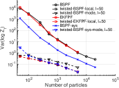
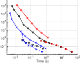
Refer to caption
Refer to caption
Fig. 2: Example A: Variance of logZtsubscript𝑍𝑡\log Z_{t} versus the number of particles n𝑛n (left) and time (right) for different particle filters. Parameters are fixed to the ground truth values. Results are averaged over 10 datasets and 30 simulations for each dataset.

We next analyze performance of the methods for generating samples using the Metropolis-Hastings PMCMC sampler. Based on the results in Fig. 2 we chose the twisted-BSPF-mode-sys and BSPF-sys as the test methods. We randomly chose one of the datasets as a test set and generated 20 000 samples using the PMMH sampler. An initial test run using the BSPF-sys with n=5000𝑛5000n=5000 particles was used to tune the proposal covariance, which was then held constant for the subsequent test runs.

Fig. 3 shows the autocorrelation performance for the methods. The BSPF-sys with n=1000𝑛1000n=1000 particles has about the same computation time as twisted-BSPF-mode-sys with n=250𝑛250n=250 particles and l=50𝑙50l=50. The twisted-BSPF-mode-sys has clearly better autocorrelation performance than the BSPF-sys with similar computation time. The effective sample sizes and relative computation times are shown in Table I. The relative computation time is obtained as the ratio of running time for each algorithm setting to that of twisted-BSPF-sys-mode with 505050 particles. Generating 20 000 samples with the twisted-BSPF-mode-sys with 50 particles took approximately 9 minutes. The twisted-BSPF-mode-sys gives clearly larger effective sample sizes in less computational time than the BSPF-sys.
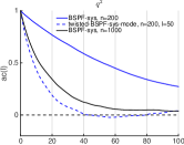
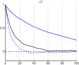
Refer to caption
Refer to caption
Refer to caption
Fig. 3: Example A: Autocorrelation plots from a MCMC chain with 20 000 samples generated using PMMH with BSPF and twisted-BSPF-mode. The autocorrelations are computed with burn in of 2500 samples excluded from the computations.
TABLE I: Example A: The average effective sample sizes and relative computation times for the different particle filters.
Particle filter n𝑛n avg.τeffavg.subscript𝜏eff\text{avg.}\;\tau_{\text{eff}} rel. time
BSPF-sys 200 167.8 0.5
500 404.6 1.0
1000 540.6 1.7
2000 753.5 3.4
twisted-BSPF-mode-sys 50 793.8 1.0
100 890.0 1.2
250 969.7 1.5
500 1019.5 2.7

The convergence of the MCMC sequence is demonstrated in Fig. 4 using normalized histograms computed from the MCMC chains. The better mixing of the MCMC chain computed using twisted-BSPF-mode-sys is especially evident in the top row histograms computed using only a small number of samples.
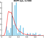
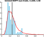
Refer to caption
Refer to caption
Refer to caption
Refer to caption
Fig. 4: Example A: Normalized histograms for parameter q2superscript𝑞2q^{2} computed from PMCMC chains using BSPF-sys with n=1000𝑛1000n=1000 (left) and twisted-BSPF-mode-sys with n=200𝑛200n=200 and l=50𝑙50l=50 (right). Number of PMCMC samples used are 500 (top row) and 2000 (bottom row). The estimated true posterior (red line) is fitted to a separate PMCMC chain with 20 000 samples. The ground truth value of the parameter is shown with a black line.

A simple demonstration of the tracking performance using the estimated parameter values is shown in Table II. We used an EKF algorithm with parameters fixed to mean values of the MCMC chains with 500 samples. The consistency value gives the fraction of times the true position is inside the 95% confidence ellipsoid, averaged over all the time steps. The 95% confidence ellipsoid at time k𝑘k is given by

(μkxtrue)T𝚺k1(μkxtrue)=Fχ221(0.95),superscriptsubscript𝜇𝑘subscript𝑥true𝑇superscriptsubscript𝚺𝑘1subscript𝜇𝑘subscript𝑥truesuperscriptsubscript𝐹superscriptsubscript𝜒2210.95(\mu_{k}-x_{\text{true}})^{T}\mathbf{\Sigma}_{k}^{-1}(\mu_{k}-x_{\text{true}})=F_{\chi_{2}^{2}}^{-1}(0.95),

where Fχ221(0.95)subscriptsuperscript𝐹1superscriptsubscript𝜒220.95F^{-1}_{\chi_{2}^{2}}(0.95) is the value of the χ2superscript𝜒2\chi^{2} inverse cumulative distribution function with 2 degrees of freedom evaluated at 0.950.950.95.

TABLE II: Example A: Tracking performance using EKF
PMCMC method RMSE 95% cons.
BSPF-sys, n=1000𝑛1000n=1000 13.2 0.92
twisted-BSPF-sys-mode, n=200𝑛200n=200, l=50𝑙50l=50 12.4 0.91

VI-B Positioning using RSS measurements

As a second example, we consider estimating the parameters of a received signal strength (RSS) measurement model in an indoor positioning scenario using Bluetooth measurements. As the user moves inside the building, the positioning device measures the attenuated signal from Bluetooth base stations situated at known locations. Given a suitable model for the signal attenuation, the measurements give information about the distance between the positioning device and the base stations. Combined with a motion model, we can then use the measurements to track the user’s movements inside the building.

For this example, we use a simple two parameter empirical model for the signal attenuation [25]. The base station specific parameters, together with any other unknown parameters (e.g. noise variances), are estimated using a learning dataset. We consider a full Bayesian approach and use the PMCMC algorithm to draw samples from the true parameter posterior distributions. The samples can then be used to compute point estimates or integrate out the parameters in subsequent positioning phases.

We use a real data set collected in a building at the Tampere University of Technology. This data consists of RSS measurements from 8 different base stations with a total of t=54𝑡54t=54 RSS measurement vectors. The locations of the base stations and the true route is shown in Fig. 5; the true route was obtained by having the user manually indicate his location on a map at regular intervals. The number of elements in the RSS measurement vector at a single time point ranges from 1 to 7, with an average number of about 5 elements per time point.
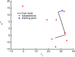
Refer to caption
Fig. 5: Example B: The indoor positioning scenario.

The dynamical model is the same as in the first example in Section VI-A. The initial state is taken to be Gaussian with mean ν0subscript𝜈0\nu_{0} and covariance 𝐏0subscript𝐏0\mathbf{P}_{0}. For this example, we fix the position components of the initial mean to the true location, and set the velocity components to zero. The initial covariance is the same as in the first example.

The measurements are modelled as

Yk=hk(Xk)+ζk,subscript𝑌𝑘subscript𝑘subscript𝑋𝑘subscript𝜁𝑘Y_{k}=h_{k}(X_{k})+\zeta_{k},

where hk(x)subscript𝑘𝑥h_{k}(x) is a vector with elements hi(x)superscript𝑖𝑥h^{i}(x), ik𝑖subscript𝑘i\in\mathcal{I}_{k}, where ksubscript𝑘\mathcal{I}_{k} contains the indices of the base stations whose RSS are measured at time k𝑘k, ζksubscript𝜁𝑘\zeta_{k} is a zero-mean Gaussian vector, independent of ωksubscript𝜔𝑘\omega_{k}, with covariance 𝐑=σ2𝐈𝐑superscript𝜎2𝐈\mathbf{R}=\sigma^{2}\mathbf{I}, and the RSS measurement function is [25]

hi(r,v)=ρi10λilog10rBS,ir,1inBS,formulae-sequencesuperscript𝑖𝑟𝑣subscript𝜌𝑖10subscript𝜆𝑖subscript10normsubscript𝑟BS𝑖𝑟1𝑖subscript𝑛BSh^{i}(r,v)=\rho_{i}-10\lambda_{i}\log_{10}\|r_{\text{BS},i}-r\|,\quad 1\leq i\leq n_{\text{BS}},

where rBS,isubscript𝑟BS𝑖r_{\text{BS},i} are the locations of measurement stations, λisubscript𝜆𝑖\lambda_{i} and ρisubscript𝜌𝑖\rho_{i} are the base station specific parameters, and nBSsubscript𝑛BSn_{\text{BS}} is the number of base stations.

The measurement likelihood is strongly non-Gaussian and can be multimodal, depending on the geometry of the base station locations. However, the term p(yk:k+l|xk)𝑝conditionalsubscript𝑦:𝑘𝑘𝑙subscript𝑥𝑘p(y_{k:k+l}\,|\,x_{k}) becomes concentrated on a single mode as the number of measurements l𝑙l increases (see Fig. 6). This allows us to reduce the computation time of the twisted particle filter by using the linearization around the mode of p(yk:k+l|xk)𝑝conditionalsubscript𝑦:𝑘𝑘𝑙subscript𝑥𝑘p(y_{k:k+l}\,|\,x_{k}), described in Section V-B, when l𝑙l is sufficiently large.

Refer to caption
Refer to caption
Refer to caption
Refer to caption
Fig. 6: Example B: Illustration of the behaviour of p(yk:k+l|xk)𝑝conditionalsubscript𝑦:𝑘𝑘𝑙subscript𝑥𝑘p(y_{k:k+l}\,|\,x_{k}) as the number of measurements l𝑙l increases. The values for l>0𝑙0l>0 are computed by running a particle filter separately for each point on a dense grid for the position rksubscript𝑟𝑘r_{k}. The velocity vksubscript𝑣𝑘v_{k} is kept fixed for this example plot.

The unknown parameters are the transition noise variance parameter q2superscript𝑞2q^{2}, the process noise variance σ2superscript𝜎2\sigma^{2}, and the measurement model parameters λisubscript𝜆𝑖\lambda_{i} and ρisubscript𝜌𝑖\rho_{i}, i=1,,nBS𝑖1subscript𝑛BSi=1,\ldots,n_{\text{BS}}. Priors for the parameters are chosen as follows. For the noise variance parameters, we use independent inverse Gamma priors 𝒢(a,b)𝒢𝑎𝑏\mathcal{IG}(a,b) with shape a𝑎a and scale b𝑏b parameters set to a=b=0.1𝑎𝑏0.1a=b=0.1 for measurement noise σ2superscript𝜎2\sigma^{2}, and to a=1𝑎1a=1 and b=0.01𝑏0.01b=0.01 for the process noise q2superscript𝑞2q^{2}. For the path-loss exponents λisubscript𝜆𝑖\lambda_{i}, we use independent gamma priors 𝒢(a,b)𝒢𝑎𝑏\mathcal{G}(a,b), with shape parameter a=3.8𝑎3.8a=3.8 and scale parameter b=1.6𝑏1.6b=1.6. For the parameters ρisubscript𝜌𝑖\rho_{i} we use independent Gaussian priors with zero mean and variance 702superscript70270^{2}.

We first determine an initial approximation for the posterior mean by generating 10 000 samples using the PMMH and BSPF with n=5000𝑛5000n=5000 particles. For this relatively high dimensional problem, we found that it was necessary to use a component-wise update, also called Metropolis-within-Gibbs, in the PMMH sampler. The parameters are updated in nBS+1subscript𝑛BS1n_{\text{BS}}+1 blocks of 2 variables, with the blocks consisting of (λi,ρi)subscript𝜆𝑖subscript𝜌𝑖(\lambda_{i},\rho_{i}), for i=1,,nBS𝑖1subscript𝑛BSi=1,\ldots,n_{\text{BS}} and (q2,σ2)superscript𝑞2superscript𝜎2(q^{2},\sigma^{2}) for the final block. For each block, we have an independent Gaussian random walk proposal, with covariance tuned during the initial PMMH run and kept fixed in the subsequent test runs.

Fig. 7 shows the variance of logZtsubscript𝑍𝑡\log Z_{t} for the twisted-BSPF-local as a function of the parameter l𝑙l, with the unknown parameters fixed to the mean values from the initial test run. It can be seen that increasing l𝑙l over 20 does not generally improve the results and can lead to larger variance of the estimate. This is most likely caused by the gradually increasing linearization errors in the computation of the twisting function using the EKF, meaning that for large l𝑙l we have a slightly poorer approximation of the optimal twisting function. For the following tests, we use a fixed l=10𝑙10l=10 for all the tested twisted particle filters.

Fig. 8 shows the variance of the different particle filters as a function of number of particles and computation time. Parameters were first fixed to the posterior mean estimate from the initial test run and then to a value chosen from the initial PMCMC chain, to test how the particle filters perform for parameter values away from the mean.

The results are similar as in the first example. All the tested twisted particle filters clearly outperform the non-twisted particle filters when looking at the number of particles needed for a specific log-likelihood variance. In a given computation time, the twisted-BSPF-mode-sys gives the lowest variance for logZtsubscript𝑍𝑡\log Z_{t}. Using systematic resampling improves the results for both twisted and non-twisted particle filters.
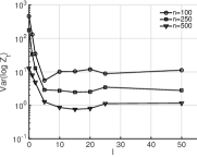
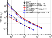
Refer to caption
Fig. 7: Example B: Variance of logZtsubscript𝑍𝑡\log Z_{t} versus the parameter l𝑙l for twisted-BSPF-local using multinomial resampling with different number of particles. Results are computed from 100 simulations.
Refer to caption
Refer to caption
Refer to caption
Refer to caption
Fig. 8: Example B: Variance of logZtsubscript𝑍𝑡\log Z_{t} versus the number of particles n𝑛n (left) and time (right) for different particle filters. Parameters are fixed to a posterior mean estimate (upper row) and to a random value chosen from test PMCMC chain (lower row). Results are computed from 500 simulations.

We proceed by comparing two of the most promising particle filters, i.e. the BSPF and twisted-BSPF-mode, in generating samples using the PMMH sampler. For each particle filter, we generated a total of 100 000 samples using 10 independent chains of 10 000 samples. Fig. 9 shows the average autocorrelation plots over the 10 chains for base station parameters λ1subscript𝜆1\lambda_{1} and ρ1subscript𝜌1\rho_{1}, and noise variances σ2superscript𝜎2\sigma^{2} and q2superscript𝑞2q^{2}. The BSPF-sys has clearly better performance compared to the BSPF with the same number of particles, as was expected from the log-likelihood variance results. However, BSPF-sys still needs a significantly larger number of particles and longer computation times (see Table III) to reach the same autocorrelation performance as twisted-BSPF-mode.

The average effective sample sizes over all the parameters and relative computation times are shown in Table III. The relative computation time is obtained as the ratio of running time for each algorithm setting to the running time of the twisted-BSPF-mode algorithm with 250250250 particles. Generating 10 000 samples with twisted-BSPF-mode with 250 particles took approximately 33 minutes.

Results show that the two tested twisted particle filters give clearly the largest effective sample size with a given number of particles and in a given computational time. For the twisted particle filters, the effect of using systematic resampling is relatively small, with the systematic resampling giving slightly better results especially for a large number of particles.
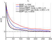
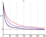
Refer to caption
Refer to caption
Refer to caption
Refer to caption
Fig. 9: Example B: Average autocorrelation plots from 10 MCMC chains generated using PMMH with BSPF and twisted-BSPF-mode. The plots are for parameters λ1subscript𝜆1\lambda_{1} (top left), ρ1subscript𝜌1\rho_{1} (top right), σ2superscript𝜎2\sigma^{2} (bottom left) and q2superscript𝑞2q^{2} (bottom right). The autocorrelations are computed from chains with 10 000 samples with burn in of 1000 samples excluded from the computations.
TABLE III: Example B: The average effective sample sizes and relative computation times for the different particle filters.
Particle filter n𝑛n avg.τeffavg.subscript𝜏eff\text{avg.}\;\tau_{\text{eff}} rel. time
BSPF 1000 59.6 1.1
2000 117.0 2.1
5000 146.0 5.7
10000 171.5 11.8
BSPF-sys 1000 81.1 0.9
2000 124.1 1.7
5000 165.5 4.5
10000 191.8 9.6
twisted-BSPF-mode 250 111.0 1.0
500 141.5 1.3
1000 162.3 2.1
2000 189.0 3.5
twisted-BSPF-sys-mode 250 110.0 1.0
500 149.6 1.3
1000 168.9 2.0
2000 199.9 3.4

A simple demonstration of the tracking performance using the estimated parameter values is shown in Table IV. We used an EKF algorithm with parameters fixed to mean values of the respective MCMC chains, computed from 10  000 MCMC samples. It should be noted that for our example, only a small amount of data was available, and for this reason the offline parameter estimation and online tracking were computed using the same data set. In reality, one would use a separate, comprehensive data set for parameter estimation.

TABLE IV: Example B: Tracking performance using EKF
PMCMC method RMSE 95% cons.
BSPF-sys, n=2000𝑛2000n=2000 4.6 0.09
twisted-BSPF-sys-mode, n=500𝑛500n=500, l=10𝑙10l=10 4.5 0.11

VII Conclusion

Our numerical results indicate that twisted particle filters can give efficiency gains for marginal likelihood approximation and parameter estimation via PMCMC. The performance gains shown in Tables I and III illustrate a speed-up of about 3-5 times for the same average effective sample size, compared to standard methods. Of course, the amount of speed-up is implementation dependent, and in our implementations we have not gone to great lengths to optimize performance of the twisted particle filter, so larger gains may well be possible. On the other hand, the efficiency of the twisted particle filter rests on the choice of the twisting functions ψksubscript𝜓𝑘\psi_{k}, and the ability to choose a “good” ψksubscript𝜓𝑘\psi_{k} is of course problem dependent.

For our purposes, a sufficient choice for ψksubscript𝜓𝑘\psi_{k} was obtained by using an EKF based linearization of the non-linear model functions. However, for problems where the EKF based methods fail to deliver a good approximation for optimal ψksubscript𝜓𝑘\psi_{k}, the presented algorithms could be modified to use linearization based on other types of Gaussian filters e.g. unscented Kalman filter or other sigma-point Gaussian filters described for example in [3].

Further research should be conducted to determine the best approach for approximating the optimal twisting function in the case of multimodal p(yk:k+l|xk)𝑝conditionalsubscript𝑦:𝑘𝑘𝑙subscript𝑥𝑘p(y_{k:k+l}\,|\,x_{k}). A possible solution could be to use mixture approximations with each component formed by linearizing the model functions around one of the modes.

There are also various other aspects of PMCMC methodology which could be developed around twisted particle filters, for example by deriving a PMMH algorithm to sample from p(θ,x0:t|y0:t)𝑝𝜃conditionalsubscript𝑥:0𝑡subscript𝑦:0𝑡p(\theta,x_{0:t}|y_{0:t}) rather than just p(θ|y0:t)𝑝conditional𝜃subscript𝑦:0𝑡p(\theta|y_{0:t}), and in deriving particle Gibbs samplers, along the lines of those introduced in [11].

Appendix A Proof of Proposition 1

Define functions (ηk)k=0tsuperscriptsubscriptsubscript𝜂𝑘𝑘0𝑡(\eta_{k})_{k=0}^{t} recursively as ηt(xt):=1assignsubscript𝜂𝑡subscript𝑥𝑡1\eta_{t}(x_{t}):=1 and ηk1(xk1):=𝕏gk(yk|xk)fk(xk|xk1)ηk(xk)𝑑xkassignsubscript𝜂𝑘1subscript𝑥𝑘1subscript𝕏subscript𝑔𝑘conditionalsubscript𝑦𝑘subscript𝑥𝑘subscript𝑓𝑘conditionalsubscript𝑥𝑘subscript𝑥𝑘1subscript𝜂𝑘subscript𝑥𝑘differential-dsubscript𝑥𝑘\eta_{k-1}(x_{k-1}):=\int_{\mathbb{X}}g_{k}(y_{k}\,|\,x_{k})f_{k}(x_{k}\,|\,x_{k-1})\eta_{k}(x_{k})\,dx_{k} for tk1𝑡𝑘1t\geq k\geq 1. For any 1kt1𝑘𝑡1\leq k\leq t we have

𝔼[Zki=1nWkiηk(ξki)i=1nWki|k1]𝔼delimited-[]conditionalsubscript𝑍𝑘superscriptsubscript𝑖1𝑛superscriptsubscript𝑊𝑘𝑖subscript𝜂𝑘superscriptsubscript𝜉𝑘𝑖superscriptsubscript𝑖1𝑛superscriptsubscript𝑊𝑘𝑖subscript𝑘1\displaystyle\mathbb{E}\left[Z_{k}\frac{\sum_{i=1}^{n}W_{k}^{i}\eta_{k}(\xi_{k}^{i})}{\sum_{i=1}^{n}W_{k}^{i}}\,\big{|}\,\mathscr{F}_{k-1}\right]
=Zk1𝔼[1ni=1n𝕏Wkiηk(ξki)qk(dξki|k1rk1i(Uk1))|k1]absentsubscript𝑍𝑘1𝔼delimited-[]conditional1𝑛superscriptsubscript𝑖1𝑛subscript𝕏superscriptsubscript𝑊𝑘𝑖subscript𝜂𝑘superscriptsubscript𝜉𝑘𝑖subscript𝑞𝑘conditional𝑑superscriptsubscript𝜉𝑘𝑖superscriptsubscript𝑘1superscriptsubscript𝑟𝑘1𝑖subscript𝑈𝑘1subscript𝑘1\displaystyle=Z_{k-1}\mathbb{E}\left[\frac{1}{n}\sum_{i=1}^{n}\int_{\mathbb{X}}W_{k}^{i}\eta_{k}(\xi_{k}^{i})q_{k}(d\xi_{k}^{i}\,|\,\mathscr{L}_{k-1}^{r_{k-1}^{i}(U_{k-1})})\,\big{|}\,\mathscr{F}_{k-1}\right]
=Zk1𝔼[1ni=1nηk1(ξk1rk1i(Uk1))|k1]absentsubscript𝑍𝑘1𝔼delimited-[]conditional1𝑛superscriptsubscript𝑖1𝑛subscript𝜂𝑘1superscriptsubscript𝜉𝑘1superscriptsubscript𝑟𝑘1𝑖subscript𝑈𝑘1subscript𝑘1\displaystyle=Z_{k-1}\mathbb{E}\left[\frac{1}{n}\sum_{i=1}^{n}\eta_{k-1}(\xi_{k-1}^{r_{k-1}^{i}(U_{k-1})})\,\big{|}\,\mathscr{F}_{k-1}\right]
=Zk1i=1nWk1iηk1(ξk1i)i=1nWk1i,absentsubscript𝑍𝑘1superscriptsubscript𝑖1𝑛superscriptsubscript𝑊𝑘1𝑖subscript𝜂𝑘1superscriptsubscript𝜉𝑘1𝑖superscriptsubscript𝑖1𝑛superscriptsubscript𝑊𝑘1𝑖\displaystyle=Z_{k-1}\frac{\sum_{i=1}^{n}W_{k-1}^{i}\eta_{k-1}(\xi_{k-1}^{i})}{\sum_{i=1}^{n}W_{k-1}^{i}}, (A.1)

where the second equality follows by plugging in Wkisuperscriptsubscript𝑊𝑘𝑖W_{k}^{i} and the final equality by using Assumption 1. We now have

𝔼[Zt]𝔼delimited-[]subscript𝑍𝑡\displaystyle\mathbb{E}[Z_{t}] =𝔼[Z0i=1nW0iη0(ξ0i)i=1nW0i]absent𝔼delimited-[]subscript𝑍0superscriptsubscript𝑖1𝑛superscriptsubscript𝑊0𝑖subscript𝜂0superscriptsubscript𝜉0𝑖superscriptsubscript𝑖1𝑛superscriptsubscript𝑊0𝑖\displaystyle=\mathbb{E}\left[Z_{0}\frac{\sum_{i=1}^{n}W_{0}^{i}\eta_{0}(\xi_{0}^{i})}{\sum_{i=1}^{n}W_{0}^{i}}\right]
=1ni=1n𝔼[W0iη0(ξ0i)]=p(y0:t),absent1𝑛superscriptsubscript𝑖1𝑛𝔼delimited-[]superscriptsubscript𝑊0𝑖subscript𝜂0superscriptsubscript𝜉0𝑖𝑝subscript𝑦:0𝑡\displaystyle=\frac{1}{n}\sum_{i=1}^{n}\mathbb{E}\left[W_{0}^{i}\eta_{0}(\xi_{0}^{i})\right]=p(y_{0:t}),

where the first equality follows by using (A.1) repeatedly and the final equality by plugging in W0isuperscriptsubscript𝑊0𝑖W_{0}^{i} and taking the expectation.

Appendix B Proof of Theorem 1

It was already established in Section IV that lines 1 to 5 in Algorithm 3 draw ξ0subscript𝜉0\xi_{0} from 𝐌~0subscript~𝐌0\widetilde{\mathbf{M}}_{0}. We next show that lines 11 to 17 in Algorithm 3 draw ξksubscript𝜉𝑘\xi_{k} and Uk1subscript𝑈𝑘1U_{k-1} from 𝐌~ksubscript~𝐌𝑘\widetilde{\mathbf{M}}_{k}. Plugging in 𝐌ksubscript𝐌𝑘\mathbf{M}_{k} to (13b) we get

𝐌~k(dξk,duk1|k1)subscript~𝐌𝑘𝑑subscript𝜉𝑘conditional𝑑subscript𝑢𝑘1subscript𝑘1\displaystyle\widetilde{\mathbf{M}}_{k}(d\xi_{k},du_{k-1}\,|\,\mathscr{F}_{k-1})
s=1n𝒰(duk1)qk(dξks|k1rk1s(uk1))ψk(k1rk1s(uk1),ξks)proportional-toabsentsuperscriptsubscript𝑠1𝑛𝒰𝑑subscript𝑢𝑘1subscript𝑞𝑘conditional𝑑superscriptsubscript𝜉𝑘𝑠superscriptsubscript𝑘1superscriptsubscript𝑟𝑘1𝑠subscript𝑢𝑘1subscript𝜓𝑘superscriptsubscript𝑘1superscriptsubscript𝑟𝑘1𝑠subscript𝑢𝑘1superscriptsubscript𝜉𝑘𝑠\displaystyle\propto\sum_{s=1}^{n}\mathcal{U}(du_{k-1})q_{k}(d\xi_{k}^{s}\,|\,\mathscr{L}_{k-1}^{r_{k-1}^{s}(u_{k-1})})\psi_{k}(\mathscr{L}_{k-1}^{r_{k-1}^{s}(u_{k-1})},\xi_{k}^{s})
isqk(dξki|k1rk1i(uk1)).\displaystyle\quad\quad\quad\quad\cdot\prod_{i\neq s}q_{k}(d\xi_{k}^{i}\,|\,\mathscr{L}_{k-1}^{r_{k-1}^{i}(u_{k-1})}). (B.1)

We recognize this as a mixture form. So to sample ξksubscript𝜉𝑘\xi_{k} and Uk1subscript𝑈𝑘1U_{k-1}, we first draw the mixture component Sksubscript𝑆𝑘S_{k} on {1,,n}1𝑛\{1,\ldots,n\} with probabilities

𝒮~k(Sk=s)[0,1]m𝒰(duk1)proportional-tosubscript~𝒮𝑘subscript𝑆𝑘𝑠subscriptsuperscript01𝑚𝒰𝑑subscript𝑢𝑘1\displaystyle\widetilde{\mathcal{S}}_{k}(S_{k}=s)\propto\int_{[0,1]^{m}}\mathcal{U}(du_{k-1})
𝕏nqk(dxks|k1rk1s(uk1)ψk(k1rk1s(uk1),xks)\displaystyle\cdot\int_{\mathbb{X}^{n}}q_{k}(dx_{k}^{s}\,|\,\mathcal{L}_{k-1}^{r_{k-1}^{s}(u_{k-1})}\psi_{k}(\mathcal{L}_{k-1}^{r_{k-1}^{s}(u_{k-1})},x_{k}^{s})
isqk(dxki|k1rk1i(uk1))\displaystyle\quad\quad\cdot\prod_{i\neq s}q_{k}(dx_{k}^{i}\,|\,\mathscr{L}_{k-1}^{r_{k-1}^{i}(u_{k-1})})
=[0,1]m𝒰(duk1)absentsubscriptsuperscript01𝑚𝒰𝑑subscript𝑢𝑘1\displaystyle=\int_{[0,1]^{m}}\mathcal{U}(du_{k-1})
𝕏qk(dxk|k1rk1s(uk1)ψk(k1rk1s(uk1),xk),\displaystyle\quad\quad\cdot\int_{\mathbb{X}}q_{k}(dx_{k}\,|\,\mathcal{L}_{k-1}^{r_{k-1}^{s}(u_{k-1})}\psi_{k}(\mathcal{L}_{k-1}^{r_{k-1}^{s}(u_{k-1})},x_{k}),

which give the probabilities in (17) and line 11 in Algorithm 3. Next we proceed to draw Uk1subscript𝑈𝑘1U_{k-1} conditional on Sk=ssubscript𝑆𝑘𝑠S_{k}=s. Given Sk=ssubscript𝑆𝑘𝑠S_{k}=s, the distribution for Uk1subscript𝑈𝑘1U_{k-1}, denoted with 𝒰~k1(|s)\widetilde{\mathcal{U}}_{k-1}(\cdot\,|\,s), is given by

𝒰~k1(duk1|s)subscript~𝒰𝑘1conditional𝑑subscript𝑢𝑘1𝑠\displaystyle\widetilde{\mathcal{U}}_{k-1}(du_{k-1}\,|\,s)
𝕏n𝒰(duk1)ψk(k1rk1s(uk1),xk)qk(dxks|k1rk1s(uk1))proportional-toabsentsubscriptsuperscript𝕏𝑛𝒰𝑑subscript𝑢𝑘1subscript𝜓𝑘superscriptsubscript𝑘1subscriptsuperscript𝑟𝑠𝑘1subscript𝑢𝑘1subscript𝑥𝑘subscript𝑞𝑘conditional𝑑superscriptsubscript𝑥𝑘𝑠superscriptsubscript𝑘1superscriptsubscript𝑟𝑘1𝑠subscript𝑢𝑘1\displaystyle\propto\int_{\mathbb{X}^{n}}\mathcal{U}(du_{k-1})\psi_{k}(\mathscr{L}_{k-1}^{r^{s}_{k-1}(u_{k-1})},x_{k})q_{k}(dx_{k}^{s}\,|\,\mathscr{L}_{k-1}^{r_{k-1}^{s}(u_{k-1})})
isqk(xki|k1rk1i(uk1))\displaystyle\quad\quad\quad\cdot\prod_{i\neq s}q_{k}(x_{k}^{i}\,|\,\mathscr{L}_{k-1}^{r_{k-1}^{i}(u_{k-1})})
=𝒰(duk1)𝕏ψk(k1rk1s(uk1),xk)qk(dxk|k1rk1s(uk1)).absent𝒰𝑑subscript𝑢𝑘1subscript𝕏subscript𝜓𝑘superscriptsubscript𝑘1subscriptsuperscript𝑟𝑠𝑘1subscript𝑢𝑘1subscript𝑥𝑘subscript𝑞𝑘conditional𝑑subscript𝑥𝑘superscriptsubscript𝑘1superscriptsubscript𝑟𝑘1𝑠subscript𝑢𝑘1\displaystyle=\mathcal{U}(du_{k-1})\int_{\mathbb{X}}\psi_{k}(\mathscr{L}_{k-1}^{r^{s}_{k-1}(u_{k-1})},x_{k})q_{k}(dx_{k}\,|\,\mathscr{L}_{k-1}^{r_{k-1}^{s}(u_{k-1})}).

This gives (18) and line 12 in Algorithm 3. Finally, given Sk=ssubscript𝑆𝑘𝑠S_{k}=s and Uk1=uk1subscript𝑈𝑘1subscript𝑢𝑘1U_{k-1}=u_{k-1}, the distribution for ξksubscript𝜉𝑘\xi_{k} is proportional to

qk(dξks|k1rk1s(uk1))ψk(k1rk1s(uk1),ξks)subscript𝑞𝑘conditional𝑑superscriptsubscript𝜉𝑘𝑠superscriptsubscript𝑘1superscriptsubscript𝑟𝑘1𝑠subscript𝑢𝑘1subscript𝜓𝑘superscriptsubscript𝑘1superscriptsubscript𝑟𝑘1𝑠subscript𝑢𝑘1superscriptsubscript𝜉𝑘𝑠\displaystyle q_{k}(d\xi_{k}^{s}\,|\,\mathscr{L}_{k-1}^{r_{k-1}^{s}(u_{k-1})})\psi_{k}(\mathscr{L}_{k-1}^{r_{k-1}^{s}(u_{k-1})},\xi_{k}^{s})
isqk(ξki|k1rk1i(uk1)).\displaystyle\cdot\prod_{i\neq s}q_{k}(\xi_{k}^{i}\,|\,\mathscr{L}_{k-1}^{r_{k-1}^{i}(u_{k-1})}).

This gives q~ksubscript~𝑞𝑘\widetilde{q}_{k} in (16) and lines 13 to 17 in Algorithm 3 for sampling ξksubscript𝜉𝑘\xi_{k}.

We next show that the expression for Z~ksubscript~𝑍𝑘\widetilde{Z}_{k} in Algorithm 3 can equivalently be written

Z~k=Zks=0kϕs,k0,formulae-sequencesubscript~𝑍𝑘subscript𝑍𝑘superscriptsubscriptproduct𝑠0𝑘subscriptitalic-ϕ𝑠𝑘0\widetilde{Z}_{k}=Z_{k}\prod_{s=0}^{k}\phi_{s},\quad k\geq 0, (B.2)

where for each 0sk0𝑠𝑘0\leq s\leq k, ϕssubscriptitalic-ϕ𝑠\phi_{s} is the Radon-Nikodym derivative d𝐌s/d𝐌~s𝑑subscript𝐌𝑠𝑑subscript~𝐌𝑠d\mathbf{M}_{s}/d\widetilde{\mathbf{M}}_{s}. The result 𝔼~[Z~k]=𝔼[Zk]~𝔼delimited-[]subscript~𝑍𝑘𝔼delimited-[]subscript𝑍𝑘\widetilde{\mathbb{E}}[\widetilde{Z}_{k}]=\mathbb{E}[Z_{k}] then immediately follows from the properties of the Radon-Nikodym derivative. Then, using Proposition 1, we get (19).

To compute the Radon-Nikodym derivatives we need to find the normalizing factors in (13a)-(13b). For k=0𝑘0k=0 the normalization factor is ψ0(x)q0(dx)subscript𝜓0𝑥subscript𝑞0𝑑𝑥\int\psi_{0}(x)q_{0}(dx) and we get

ϕ0(ξ0)subscriptitalic-ϕ0subscript𝜉0\displaystyle\phi_{0}(\xi_{0}) =d𝐌0()d𝐌~0()(ξ0)=𝕏ψ0(x0)q0(dx0)1ni=1nψ0(ξ0i).absent𝑑subscript𝐌0𝑑subscript~𝐌0subscript𝜉0subscript𝕏subscript𝜓0subscript𝑥0subscript𝑞0𝑑subscript𝑥01𝑛superscriptsubscript𝑖1𝑛subscript𝜓0superscriptsubscript𝜉0𝑖\displaystyle=\frac{d\mathbf{M}_{0}(\cdot)}{d\widetilde{\mathbf{M}}_{0}(\cdot)}(\xi_{0})=\frac{\int_{\mathbb{X}}\psi_{0}(x_{0})q_{0}(dx_{0})}{\frac{1}{n}\sum_{i=1}^{n}\psi_{0}(\xi_{0}^{i})}. (B.3)

For k>0𝑘0k>0, the normalization factor is given by

[0,1]m𝕏n1ns=1n𝐌k(dξk,duk1|k1)subscriptsuperscript01𝑚subscriptsuperscript𝕏𝑛1𝑛superscriptsubscript𝑠1𝑛subscript𝐌𝑘𝑑subscript𝜉𝑘conditional𝑑subscript𝑢𝑘1subscript𝑘1\displaystyle\int_{[0,1]^{m}}\int_{\mathbb{X}^{n}}\frac{1}{n}\sum_{s=1}^{n}\mathbf{M}_{k}(d\xi_{k},d{u_{k-1}}\,|\,\mathscr{F}_{k-1})
ψk(k1rk1s(uk1),ξks)absentsubscript𝜓𝑘superscriptsubscript𝑘1superscriptsubscript𝑟𝑘1𝑠subscript𝑢𝑘1superscriptsubscript𝜉𝑘𝑠\displaystyle\quad\quad\quad\quad\cdot\psi_{k}(\mathscr{L}_{k-1}^{r_{k-1}^{s}(u_{k-1})},\xi_{k}^{s})
=[0,1]m𝒰(duk1)absentsubscriptsuperscript01𝑚𝒰𝑑subscript𝑢𝑘1\displaystyle=\int_{[0,1]^{m}}\mathcal{U}(du_{k-1})
1ns=1n𝕏ψk(k1rk1s(uk1),xk)qk(dxk|k1rk1s(uk1))absent1𝑛superscriptsubscript𝑠1𝑛subscript𝕏subscript𝜓𝑘superscriptsubscript𝑘1subscriptsuperscript𝑟𝑠𝑘1subscript𝑢𝑘1subscript𝑥𝑘subscript𝑞𝑘conditional𝑑subscript𝑥𝑘superscriptsubscript𝑘1superscriptsubscript𝑟𝑘1𝑠subscript𝑢𝑘1\displaystyle\quad\quad\cdot\frac{1}{n}\sum_{s=1}^{n}\int_{\mathbb{X}}\psi_{k}(\mathscr{L}_{k-1}^{r^{s}_{k-1}(u_{k-1})},x_{k})q_{k}(dx_{k}\,|\,\mathscr{L}_{k-1}^{r_{k-1}^{s}(u_{k-1})})
=𝔼[1ns=1n𝕏ψk(k1rk1s(Uk1),xk)\displaystyle=\mathbb{E}\left[\frac{1}{n}\sum_{s=1}^{n}\int_{\mathbb{X}}\psi_{k}(\mathscr{L}_{k-1}^{r^{s}_{k-1}(U_{k-1})},x_{k})\right.
qk(dxk|k1rk1s(Uk1))|k1]\displaystyle\quad\quad\quad\quad\quad\quad\left.\left.\cdot q_{k}(dx_{k}\,|\,\mathscr{L}_{k-1}^{r_{k-1}^{s}(U_{k-1})})\,\right|\,\mathscr{F}_{k-1}\right]
=i=1nWk1i𝕏ψk(k1i,xk)qk(dxk|k1i)i=1nWk1iabsentsuperscriptsubscript𝑖1𝑛superscriptsubscript𝑊𝑘1𝑖subscript𝕏subscript𝜓𝑘superscriptsubscript𝑘1𝑖subscript𝑥𝑘subscript𝑞𝑘conditional𝑑subscript𝑥𝑘superscriptsubscript𝑘1𝑖superscriptsubscript𝑖1𝑛superscriptsubscript𝑊𝑘1𝑖\displaystyle=\frac{\sum_{i=1}^{n}W_{k-1}^{i}\int_{\mathbb{X}}\psi_{k}(\mathscr{L}_{k-1}^{i},x_{k})q_{k}(dx_{k}\,|\,\mathscr{L}_{k-1}^{i})}{\sum_{i=1}^{n}W_{k-1}^{i}}
=i=1nW~k1ii=1nWk1iabsentsuperscriptsubscript𝑖1𝑛superscriptsubscript~𝑊𝑘1𝑖superscriptsubscript𝑖1𝑛superscriptsubscript𝑊𝑘1𝑖\displaystyle=\frac{\sum_{i=1}^{n}\widetilde{W}_{k-1}^{i}}{\sum_{i=1}^{n}W_{k-1}^{i}}

where we used Assumption 1 and W~k1isuperscriptsubscript~𝑊𝑘1𝑖\widetilde{W}_{k-1}^{i} are given by (14). The Radon-Nikodym derivative for k>0𝑘0k>0 is now found to be

ϕk(k1,ξk)subscriptitalic-ϕ𝑘subscript𝑘1subscript𝜉𝑘\displaystyle\phi_{k}(\mathscr{F}_{k-1},\xi_{k}) =d𝐌k(|k1)d𝐌~k(|k1)(ξk)\displaystyle=\frac{d\mathbf{M}_{k}(\cdot\,|\,\mathscr{F}_{k-1})}{d\widetilde{\mathbf{M}}_{k}(\cdot\,|\,\mathscr{F}_{k-1})}(\xi_{k})
=i=1nW~k1ii=1nWk1i11ni=1nψk(ki).absentsuperscriptsubscript𝑖1𝑛superscriptsubscript~𝑊𝑘1𝑖superscriptsubscript𝑖1𝑛superscriptsubscript𝑊𝑘1𝑖11𝑛superscriptsubscript𝑖1𝑛subscript𝜓𝑘superscriptsubscript𝑘𝑖\displaystyle=\frac{\sum_{i=1}^{n}\widetilde{W}_{k-1}^{i}}{\sum_{i=1}^{n}W_{k-1}^{i}}\frac{1}{\frac{1}{n}\sum_{i=1}^{n}\psi_{k}(\mathscr{L}_{k}^{i})}. (B.4)

Writing out the expression for Z~ksubscript~𝑍𝑘\widetilde{Z}_{k} from Algorithm 3 and using the expression for Zksubscript𝑍𝑘Z_{k} from Algorithm 2, we have

Z~0subscript~𝑍0\displaystyle\widetilde{Z}_{0} =i=1nW0i𝕏ψ0(x0)q0(dx0)j=1nψ0(ξ0j)=Z0𝕏ψ0(x0)q0(dx0)1nj=1nψ0(ξ0j),absentsuperscriptsubscript𝑖1𝑛superscriptsubscript𝑊0𝑖subscript𝕏subscript𝜓0subscript𝑥0subscript𝑞0𝑑subscript𝑥0superscriptsubscript𝑗1𝑛subscript𝜓0superscriptsubscript𝜉0𝑗subscript𝑍0subscript𝕏subscript𝜓0subscript𝑥0subscript𝑞0𝑑subscript𝑥01𝑛superscriptsubscript𝑗1𝑛subscript𝜓0superscriptsubscript𝜉0𝑗\displaystyle=\dfrac{\sum_{i=1}^{n}W_{0}^{i}\int_{\mathbb{X}}\psi_{0}(x_{0})q_{0}(dx_{0})}{\sum_{j=1}^{n}\psi_{0}(\xi_{0}^{j})}=Z_{0}\dfrac{\int_{\mathbb{X}}\psi_{0}(x_{0})q_{0}(dx_{0})}{\frac{1}{n}\sum_{j=1}^{n}\psi_{0}(\xi_{0}^{j})}, (B.5)

and for k>0𝑘0k>0

Z~k=Z~0i=1nWkii=1nW0is=1ki=1nW~s1ii=1nψs(si)subscript~𝑍𝑘subscript~𝑍0superscriptsubscript𝑖1𝑛superscriptsubscript𝑊𝑘𝑖superscriptsubscript𝑖1𝑛superscriptsubscript𝑊0𝑖superscriptsubscriptproduct𝑠1𝑘superscriptsubscript𝑖1𝑛superscriptsubscript~𝑊𝑠1𝑖superscriptsubscript𝑖1𝑛subscript𝜓𝑠superscriptsubscript𝑠𝑖\displaystyle\widetilde{Z}_{k}=\widetilde{Z}_{0}\frac{\sum_{i=1}^{n}W_{k}^{i}}{\sum_{i=1}^{n}W_{0}^{i}}\prod_{s=1}^{k}\frac{\sum_{i=1}^{n}\widetilde{W}_{s-1}^{i}}{\sum_{i=1}^{n}\psi_{s}(\mathscr{L}_{s}^{i})}
=Zk𝕏ψ0(x0)q0(dx0)j=1nψ0(ξ0j)s=1ki=1nW~s1ii=1nWs1i11ni=1nψs(si),absentsubscript𝑍𝑘subscript𝕏subscript𝜓0subscript𝑥0subscript𝑞0𝑑subscript𝑥0superscriptsubscript𝑗1𝑛subscript𝜓0superscriptsubscript𝜉0𝑗superscriptsubscriptproduct𝑠1𝑘superscriptsubscript𝑖1𝑛superscriptsubscript~𝑊𝑠1𝑖superscriptsubscript𝑖1𝑛superscriptsubscript𝑊𝑠1𝑖11𝑛superscriptsubscript𝑖1𝑛subscript𝜓𝑠superscriptsubscript𝑠𝑖\displaystyle=Z_{k}\dfrac{\int_{\mathbb{X}}\psi_{0}(x_{0})q_{0}(dx_{0})}{\sum_{j=1}^{n}\psi_{0}(\xi_{0}^{j})}\prod_{s=1}^{k}\frac{\sum_{i=1}^{n}\widetilde{W}_{s-1}^{i}}{\sum_{i=1}^{n}W_{s-1}^{i}}\frac{1}{\frac{1}{n}\sum_{i=1}^{n}\psi_{s}(\mathscr{L}_{s}^{i})}, (B.6)

and combining (B.5)-(B.6) with (B.3)-(B.4) we observe that (B.2) holds as claimed.

Appendix C Proof of Theorem 2

With this choice of twisting function, we have the following result for 0kt10𝑘𝑡10\leq k\leq t-1

W~kisuperscriptsubscript~𝑊𝑘𝑖\displaystyle\widetilde{W}_{k}^{i} =Wki𝕏ψk+1(ki,xk+1)qk+1(xk+1|ki)𝑑xk+1absentsuperscriptsubscript𝑊𝑘𝑖subscript𝕏subscript𝜓𝑘1superscriptsubscript𝑘𝑖subscript𝑥𝑘1subscript𝑞𝑘1conditionalsubscript𝑥𝑘1superscriptsubscript𝑘𝑖differential-dsubscript𝑥𝑘1\displaystyle=W_{k}^{i}\int_{\mathbb{X}}\psi_{k+1}(\mathscr{L}_{k}^{i},x_{k+1})q_{k+1}(x_{k+1}\,|\,\mathscr{L}_{k}^{i})\,dx_{k+1}
=Wki𝕏fk+1(xk+1|ξki)p(yk+1:T|xk+1)𝑑xk+1absentsuperscriptsubscript𝑊𝑘𝑖subscript𝕏subscript𝑓𝑘1conditionalsubscript𝑥𝑘1superscriptsubscript𝜉𝑘𝑖𝑝conditionalsubscript𝑦:𝑘1𝑇subscript𝑥𝑘1differential-dsubscript𝑥𝑘1\displaystyle=W_{k}^{i}\int_{\mathbb{X}}f_{k+1}(x_{k+1}\,|\,\xi_{k}^{i})p(y_{k+1:T}\,|\,x_{k+1})\,dx_{k+1}
=Wki𝕏p(yk+1:T,xk+1|ξki)𝑑xk+1absentsuperscriptsubscript𝑊𝑘𝑖subscript𝕏𝑝subscript𝑦:𝑘1𝑇conditionalsubscript𝑥𝑘1superscriptsubscript𝜉𝑘𝑖differential-dsubscript𝑥𝑘1\displaystyle=W_{k}^{i}\int_{\mathbb{X}}p(y_{k+1:T},x_{k+1}\,|\,\xi_{k}^{i})\,dx_{k+1}
=Wkip(yk+1:t|ξki)=ψk(ki).absentsuperscriptsubscript𝑊𝑘𝑖𝑝conditionalsubscript𝑦:𝑘1𝑡superscriptsubscript𝜉𝑘𝑖subscript𝜓𝑘superscriptsubscript𝑘𝑖\displaystyle=W_{k}^{i}\,p(y_{k+1:t}\,|\,\xi_{k}^{i})=\psi_{k}(\mathscr{L}_{k}^{i}).

The final step follows by plugging in Wkisuperscriptsubscript𝑊𝑘𝑖W_{k}^{i} and noting that gk(yk|ξki)p(yk+1:t|ξki)=p(yk:t|ξki)subscript𝑔𝑘conditionalsubscript𝑦𝑘superscriptsubscript𝜉𝑘𝑖𝑝conditionalsubscript𝑦:𝑘1𝑡superscriptsubscript𝜉𝑘𝑖𝑝conditionalsubscript𝑦:𝑘𝑡superscriptsubscript𝜉𝑘𝑖g_{k}(y_{k}\,|\,\xi_{k}^{i})p(y_{k+1:t}\,|\,\xi_{k}^{i})=p(y_{k:t}\,|\,\xi_{k}^{i}). Furthermore, for k=t𝑘𝑡k=t, we have ψt(ti)=Wtisubscript𝜓𝑡superscriptsubscript𝑡𝑖superscriptsubscript𝑊𝑡𝑖\psi_{t}(\mathscr{L}_{t}^{i})=W_{t}^{i}.

Expanding and rearranging terms in the expression for Z~tsubscript~𝑍𝑡\widetilde{Z}_{t} in Algorithm 3 we get

Z~tsubscript~𝑍𝑡\displaystyle\widetilde{Z}_{t} =𝕏q0(dx0)ψ0(x0)k=0t1i=1nWkii=0nψk(ki)i=1nW~kii=1nWkiabsentsubscript𝕏subscript𝑞0𝑑subscript𝑥0subscript𝜓0subscript𝑥0superscriptsubscriptproduct𝑘0𝑡1superscriptsubscript𝑖1𝑛superscriptsubscript𝑊𝑘𝑖superscriptsubscript𝑖0𝑛subscript𝜓𝑘superscriptsubscript𝑘𝑖superscriptsubscript𝑖1𝑛superscriptsubscript~𝑊𝑘𝑖superscriptsubscript𝑖1𝑛superscriptsubscript𝑊𝑘𝑖\displaystyle=\int_{\mathbb{X}}q_{0}(dx_{0})\psi_{0}(x_{0})\prod_{k=0}^{t-1}\frac{\sum_{i=1}^{n}W_{k}^{i}}{\sum_{i=0}^{n}\psi_{k}{(\mathscr{L}_{k}^{i})}}\frac{\sum_{i=1}^{n}\widetilde{W}_{k}^{i}}{\sum_{i=1}^{n}W_{k}^{i}}
i=1nWti=1nψt(ti)absentsuperscriptsubscript𝑖1𝑛subscript𝑊𝑡superscriptsubscript𝑖1𝑛subscript𝜓𝑡superscriptsubscript𝑡𝑖\displaystyle\quad\quad\cdot\frac{\sum_{i=1}^{n}W_{t}}{\sum_{i=1}^{n}\psi_{t}(\mathscr{L}_{t}^{i})}
=𝕏q0(dx0)ψ0(x0)k=0t1i=1nW~kii=1nψk(ki)i=1nWti=1nψt(ti)absentsubscript𝕏subscript𝑞0𝑑subscript𝑥0subscript𝜓0subscript𝑥0superscriptsubscriptproduct𝑘0𝑡1superscriptsubscript𝑖1𝑛superscriptsubscript~𝑊𝑘𝑖superscriptsubscript𝑖1𝑛subscript𝜓𝑘superscriptsubscript𝑘𝑖superscriptsubscript𝑖1𝑛subscript𝑊𝑡superscriptsubscript𝑖1𝑛subscript𝜓𝑡superscriptsubscript𝑡𝑖\displaystyle=\int_{\mathbb{X}}q_{0}(dx_{0})\psi_{0}(x_{0})\prod_{k=0}^{t-1}\frac{\sum_{i=1}^{n}\widetilde{W}_{k}^{i}}{\sum_{i=1}^{n}\psi_{k}{(\mathscr{L}_{k}^{i})}}\frac{\sum_{i=1}^{n}W_{t}}{\sum_{i=1}^{n}\psi_{t}(\mathscr{L}_{t}^{i})}
=𝕏μ0(dx0)p(y0:t|x0)=p(y0:t).absentsubscript𝕏subscript𝜇0𝑑subscript𝑥0𝑝conditionalsubscript𝑦:0𝑡subscript𝑥0𝑝subscript𝑦:0𝑡\displaystyle=\int_{\mathbb{X}}\mu_{0}(dx_{0})p(y_{0:t}\,|\,x_{0})=p(y_{0:t}).

Acknowledgment

J. Ala-Luhtala acknowledges financial support from the Tampere University of Technology Doctoral Programme in Engineering and Natural Sciences, Emil Aaltonen foundation and KAUTE foundation. N. Whiteley and K. Heine were partly supported by EPSRC grant EP/K023330/1 and SuSTaIn.

References

  • [1] N. Whiteley and A. Lee, “Twisted particle filters,” Ann. Stat., vol. 42, no. 1, pp. 115–141, 2014.
  • [2] Y. Bar-Shalom, X. R. Li, and T. Kirubarajan, Estimation with Applications to Tracking and Navigation: Theory, Algorithms and Software.   John Wiley & Sons, 2004.
  • [3] S. Särkkä, Bayesian Filtering and Smoothing.   Cambridge University Press, 2013.
  • [4] B. Ristic, S. Arulampalm, and N. J. Gordon, Beyond the Kalman filter: Particle filters for tracking applications.   Artech House Publishers, 2004.
  • [5] T. B. Schön, A. Wills, and B. Ninness, “System identification of nonlinear state-space models,” Automatica, vol. 47, no. 1, pp. 39–49, 2011.
  • [6] O. Cappé, E. Moulines, and T. Ryden, Inference in Hidden Markov Models.   Springer, 2005.
  • [7] C. P. Casella and G. Casella, Monte Carlo Statistical methods.   Springer, 1999.
  • [8] M. A. Beaumont, “Estimation of population growth or decline in genetically monitored populations.” Genetics, vol. 164, no. 3, pp. 1139–1160, Jul. 2003. [Online]. Available: http://www.ncbi.nlm.nih.gov/pmc/articles/PMC1462617/
  • [9] C. Andrieu and G. O. Roberts, “The pseudo-marginal approach for efficient Monte Carlo computations,” Ann. Stat., vol. 37, no. 2, pp. 697–725, 2009.
  • [10] N. J. Gordon, D. J. Salmond, and A. F. Smith, “Novel approach to nonlinear/non-Gaussian Bayesian state estimation,” in IEE Proc. F (Radar and Signal Processing), vol. 140, no. 2.   IET, 1993, pp. 107–113.
  • [11] C. Andrieu, A. Doucet, and R. Holenstein, “Particle Markov chain Monte Carlo methods,” J. R. Stat. Soc. Series B (Stat. Methodol.), vol. 72, no. 3, pp. 269–342, 2010.
  • [12] C. Andrieu and M. Vihola, “Convergence properties of pseudo-marginal Markov chain Monte Carlo algorithms,” Ann. Appl. Probab., vol. 25, no. 2, pp. 1030–1077, Apr. 2015. [Online]. Available: http://dx.doi.org/10.1214/14-AAP1022
  • [13] A. Doucet, S. Godsill, and C. Andrieu, “On sequential Monte Carlo sampling methods for Bayesian filtering,” Stat. Comput., vol. 10, no. 3, pp. 197–208, 2000.
  • [14] M. K. Pitt and N. Shephard, “Filtering via simulation: Auxiliary particle filters,” J. Am. Stat. Assoc., vol. 94, no. 446, pp. 590–599, 1999.
  • [15] F. Gustafsson, F. Gunnarsson, N. Bergman, U. Forssell, J. Jansson, R. Karlsson, and P.-J. Nordlund, “Particle filters for positioning, navigation, and tracking,” IEEE Trans. Signal Process., vol. 50, no. 2, pp. 425–437, 2002.
  • [16] N. Patwari, J. N. Ash, S. Kyperountas, A. O. Hero III, R. L. Moses, and N. S. Correal, “Locating the nodes: cooperative localization in wireless sensor networks,” IEEE Signal Process Mag., vol. 22, no. 4, pp. 54–69, 2005.
  • [17] X. Li, “RSS-based location estimation with unknown pathloss model,” IEEE Trans. Wireless Commun., vol. 5, no. 12, pp. 3626–3633, Dec. 2006.
  • [18] G. Wang, H. Chen, Y. Li, and M. Jin, “On received-signal-strength based localization with unknown transmit power and path loss exponent,” IEEE Wireless Commun. Lett., vol. 1, no. 5, pp. 536–539, Oct. 2012.
  • [19] V. Seshadri, G. V. Zaruba, and M. Huber, “A Bayesian sampling approach to in-door localization of wireless devices using received signal strength indication,” in Proc. 3rd IEEE Int. Conf. on Pervasive Comput. and Commun. (PerCom 2005).   IEEE, 2005, pp. 75–84.
  • [20] R. Douc and O. Cappé, “Comparison of resampling schemes for particle filtering,” in Proc. 4th Int. Symp. Image and Signal Process. and Anal. (ISPA 2005).   IEEE, Sep. 2005, pp. 64–69.
  • [21] K. B. Athreya, “Change of measures for Markov chains and the LlogL theorem for branching processes,” Bernoulli, vol. 6, no. 2, pp. 323–338, 2000. [Online]. Available: http://projecteuclid.org/euclid.bj/1081788031
  • [22] O. Hlinka, O. Slučiak, F. Hlawatsch, P. M. Djurić, and M. Rupp, “Likelihood consensus and its application to distributed particle filtering,” IEEE Trans. Signal Process., vol. 60, no. 8, pp. 4334–4349, 2012.
  • [23] S. Ali-Löytty and N. Sirola, “Gaussian mixture filter in hybrid navigation,” in Proc. Europ. Nav. Conf. (GNSS 2007), Switzerland, May 2007, pp. 831–837. [Online]. Available: http://math.tut.fi/posgroup/aliloyttyENC2007a.pdf
  • [24] R. E. Kass, B. P. Carlin, A. Gelman, and R. M. Neal, “Markov chain Monte Carlo in practice: A roundtable discussion,” Am. Stat., vol. 52, no. 2, pp. 93–100, 1998.
  • [25] M. Hatay, “Empirical formula for propagation loss in land mobile radio services,” IEEE Trans. Veh. Technol., vol. 29, no. 3, pp. 317–325, Aug. 1980.