Isotropization of the universe during inflation

Abstract

A primordial inflationary phase allows one to erase any possible anisotropic expansion thanks to the cosmic no-hair theorem. If there is no global anisotropic stress, then the anisotropic expansion rate tends to decrease. What are the observational consequences of a possible early anisotropic phase? We first review the dynamics of anisotropic universes and report analytic approximations. We then discuss the structure of dynamical equations for perturbations and the statistical properties of observables, as well as the implication of a primordial anisotropy on the quantization of these perturbations during inflation. Finally we briefly review models based on primordial vector field which evade the cosmic no-hair theorem.

I Introduction

For good or for evil, inflation is currently the only known mechanism capable of explaining the origin and statistical properties of large scale structures in the universe. Given its central role on the standard cosmological model, it is thus important to test its robustness in all possible ways.

Even though inflation was designed, among other things, to wash away classical inhomogeneities Guth:1980zm , most of its implementations start with a symmetric background from the onset. This approach was mainly supported by large field models in which a long period of exponential expansion takes place Linde:2007fr , thus effectively erasing all possible memories of initial conditions. However, if inflationary models predicting a small number of e-folds turn out to be favoured, then the state of the universe before the onset of inflation can play an important role for cosmological observables, and thus they need to be included in a self-consistent way.

From an observational perspective, the question of the relevance of pre-inflationary initial conditions was boosted by the detection of large-scale statistical anomalies in the cosmic microwave background (CMB) temperature maps Bennett:2010jb ; Ade:2013nlj ; Ade:2015hxq . If inflation is sensitive to the initial conditions such as spatial inhomogeneities, then these features could be imprinted on the primordial power spectrum at large scales, and thus possibly related to the origin of CMB anomalies.

As it turns out, the implementation of inflation in a broader geometrical framework leads to several important questions, including the very possibility of an inflating universe in the presence of large inhomogeneities Goldwirth:1990pm ; Deruelle:1994pa . In this review paper, we address the implementation of slow-roll inflation without assuming some of the symmetries that the mechanism is supposed to predict. Specifically, we investigate the dynamics of the inflaton when released in an spatially homogeneous but anisotropic spacetime of the Bianchi I family. We show that the existence of an adiabatic (Bunch Davies) vacuum cannot be guaranteed throughout the anisotropic phase, and thus that the amplitude of strongly anisotropic modes cannot be unambiguously fixed.

This review is organized as follows: we start by recalling the basic equations and definitions of Bianchi I spacetimes in II.1 We then use these equations to find analytical solutions for the geometry in the presence of a cosmological constant in II.2. Using these solutions, we conduct a semi-analytical investigation of the inflationary dynamics using the chaotic potential as a proxy in II.3. In III we discuss the quantizations procedures (III.1), the general properties of linear perturbations (III.2), and the connection between anisotropic inflation and CMB anomalies (III.3). In IV 4 we briefly comment on some alternative models, including vector and shear-free anisotropic inflation.

Throughout this text, Latin/Greek indices refer to space/spacetime coordinates. Moreover, we adopt the convention in which indices separated by square brackets are not summed over. So, for example, $[a_{i}]\delta^{i}_{j}$ carries no sum in $i$, whereas $a_{i}\delta^{i}_{j}$ does.

II Inflation in Bianchi I spacetimes

II.1 Background generalities

We start by studying inflation in Bianchi I (BI) spacetimes. These are exact solutions of Einstein equations describing homogeneous but anisotropically expanding spacetimes with flat spatial sections. In comoving coordinates, their metric is given by

$${{\rm d}}s^{2}=-{\rm d}\tau^{2}+S^{2}(\tau)\gamma_{ij}(\tau){\rm d}x^{i}{\rm d}x^{j}\,,$$ (1)

where $\tau$ is the time measured by comoving observers, $\gamma_{ij}$ is the metric on constant-time hypersurfaces, parametrized by

$$\gamma_{ij}(\tau)=\exp[2\beta_{i}(\tau)]\delta_{ij}\,.$$ (2)

$S$ is the (geometrical) average of the three individual scale factors $X_{i}\equiv Se^{\beta_{i}}$, since

$$S\equiv(X_{1}X_{2}X_{3})^{1/3}.$$ (3)

The functions $\beta_{i}(\tau)$ are not independent, but constrained by

$$\sum_{i=1}^{3}\beta_{i}=0\,,$$ (4)

which ensures that spatial comoving volumes are constant in time ($\sqrt{\gamma}=1$). Anisotropic expansion induces a geometrical shear, which is described by the shear tensor and shear scalar

$${\hat{\sigma}}^{i}_{j}\equiv[\dot{\beta}_{i}]\delta^{i}_{j}\,,\quad{\hat{\sigma}}^{2}\equiv{\hat{\sigma}}^{i}_{j}{\hat{\sigma}}^{j}_{i}\,,$$ (5)

where a dot means ${\rm d}/{\rm d}\tau$ and spatial indices are lowered by $\gamma_{ij}$ and raised with its inverse $\gamma^{ij}$.

In the presence of a perfect fluid of energy density $\rho$ and pressure $p$, the background Einstein equations are

$$3H^{2} =\kappa\rho+\frac{1}{2}\hat{\sigma}^{2}\,,$$ (6)

$$\frac{\ddot{S}}{S} =-\frac{\kappa}{6}(\rho+3p)-\frac{1}{3}\hat{\sigma}^{2}\,,$$ (7)

$$(\hat{\sigma}^{i}_{j})^{\raisebox{-0.75346pt}{\scalebox{1.2}{$\cdot$}}} =-3H\hat{\sigma}^{i}_{j}\,.$$ (8)

where $H\equiv\dot{S}/S$ is the (average) Hubble parameter. These equations can be combined to recover the fluid conservation equation $\dot{\rho}+3H(\rho+p)=0$. Since there are no sources for the stress dynamics, Eq. (8) implies that the shear has only a decaying mode

$${\hat{\sigma}}^{i}_{j}=\frac{[C_{i}]}{S^{3}}\delta^{i}_{j}\,,\quad{\hat{\sigma}}^{2}=\frac{C^{2}}{S^{6}}\,.$$ (9)

The constants $C_{i}$ can be parametrized by

$$C_{i}=\sqrt{\frac{2}{3}}C\sin\alpha_{i}\,,\quad\alpha_{i}=\alpha+i\frac{2\pi}{3}\,,$$ (10)

which automatically ensures that $\sum_{i}C_{i}=0$ and $C^{2}=\sum_{i}C_{i}^{2}$. Clearly, $C$ measures the initial amplitude of the shear. The constant $\alpha$, on the other hand, represents a residual freedom in the choice of the initially expanding/contracting eigendirections of the shear. Before moving on, we note from Eqs. (5) and (9) that $\beta_{i}$ can be written as

$$\beta_{i}(\tau)=C_{i}\int^{\tau}\frac{{\rm d}\tau^{\prime}}{S^{3}(\tau^{\prime})}\,.$$ (11)

This expression will be useful in finding analytical solutions of the anisotropic phase.

II.2 “de Sitter” expansion

Before going into the details of slow-roll inflation in BI spacetimes, it is rewarding to analyse the expansion in the presence of a pure cosmological constant, for which solutions can be found analytically Pitrou:2008gk . These solutions keep most of the main features that are found in the more general (slow-roll inflation) case. From the behaviour of Eqs. (6) and (9), we see that the universe starts from a shear-dominated phase, followed by a (nearly) de Sitter expansion. Setting $\kappa\rho=\Lambda$ in Eq. (6) and integrating, we find that Moss:1986ud ; Pitrou:2008gk

$$S(\tau)=\left[\sqrt{\frac{3}{2}}C\tau_{\Lambda}\sinh(\tau/\tau_{\Lambda})\right]^{1/3}\,,$$ (12)

with the typical time scale $\tau_{\Lambda}\equiv(3\Lambda)^{-1/2}$. The average Hubble parameter then becomes

$$H=\frac{1}{3\tau_{\Lambda}}\coth\left(\frac{\tau}{\tau_{\Lambda}}\right)\,.$$ (13)

For $\tau\gg\tau_{\Lambda}$, $\coth(\tau/\tau_{\Lambda})$ approaches 1 and we recover $3H^{2}\approx\Lambda$, as expected. Thus, $\tau_{\Lambda}$ is the typical duration of a primordial anisotropic phase prior to a “pure” de Sitter expansion. The isotropization is better illustrated by plotting the directional scale factors, which can be obtained by integrating Eq. (11)

$$\beta_{i}(\tau)=\log\left[\tanh\left(\frac{\tau}{2\tau_{\Lambda}}\right)\right]^{\frac{2}{3}\sin\alpha_{i}}$$ (14)

and using the definition (3). With this, we find that the individual scale factors evolve as

$$X_{i}=S(\tau)\left[\tanh\left(\frac{\tau}{2\tau_{\Lambda}}\right)\right]^{\frac{2}{3}\sin\alpha_{i}}\,.$$ (15)

We plot in Figure 1 the typical behaviour of these scale factors, on which the isotropization process is obvious. Because of the condition (4), there will always exist one bouncing direction, except for the case of $\alpha=\pi/2$. The case $\alpha=\pi/2$ is necessarily exceptional since it is the only model for which the invariant $R_{\alpha\beta\mu\nu}R^{\alpha\beta\mu\nu}$ is finite as $\tau\rightarrow 0$. Since this invariant diverges at the singularity for any other $\alpha$, we conclude that the case $\alpha=\pi/2$ is singular Pitrou:2008gk . In fact, in absence of a cosmological constant ($\Lambda=0$), it also corresponds to a patch of the Minkowski spacetime Kofman:2011tr .

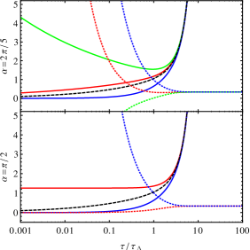
Figure 1: Three directional scale factors (thick, continuous lines) as a function of time for two values of $\alpha$. Note that they all converge to the mean scale factor (thick, dashed line). We also show the directional Hubble parameters, $\dot{X}_{i}/X_{i}$ (thin, dotted lines).

II.3 Slow-roll inflation

We are primarily interested in the inflationary dynamics on a BI spacetime geometry. We thus assume that the inflaton is described by a single, canonical scalar field with energy-momentum tensor

$$T_{\mu\nu}=\partial_{\mu}\varphi\partial_{\nu}\varphi-\frac{1}{2}\left(\partial_{\lambda}\varphi\partial^{\lambda}\varphi+2V\right)g_{\mu\nu}\,.$$

For simplicity we will focus on the model of chaotic inflation Linde:1983gd

$$V(\varphi)=\frac{1}{2}m^{2}\varphi^{2}\,.$$ (16)

We stress however that most of our results can be easily extended to other potentials.

For a homogeneous field, $\varphi=\varphi(\tau)$, the Klein-Gordon equation involves only the trace of the spatial metric. Thus, the dynamics of $\varphi$ is formally the same as in Friedmann-Lemaître (FL), i.e. isotropic universes, that is

$$\ddot{\varphi}+3H\dot{\varphi}+V_{,\varphi}=0\,.$$ (17)

However, we must stress that the (average) Hubble parameter is affected by the presence of shear, which indirectly affects $\varphi$. In what follows it will be convenient to define a dimensionless parameter $x\equiv{\hat{\sigma}}/\sqrt{6}H$. In terms of $x$, Eq. (6) becomes

$$(1-x^{2})H^{2}=\frac{\kappa}{3}\rho$$ (18)

and it implies that $x<1$ in order to ensure that the energy density is positive. We also introduce two slow-roll parameters as follows

$$\epsilon\equiv\frac{3}{2}\dot{\varphi}^{2}\left[\frac{1}{2}\dot{\varphi}^{2}+V\right]^{-1},\quad\delta\equiv-\frac{\ddot{\varphi}}{H\dot{\varphi}}\,.$$ (19)

In standard inflation, the dynamics of the universe is characterized by an attractor (slow-roll) regime in which both $\epsilon$ and $\delta$ are small and their time derivatives behave as ${\cal O}(\epsilon^{2},\epsilon\delta)$ peter2013primordial . The main effect of the spatial anisotropy is to introduce a second attractor regime in the inflationary dynamics. Indeed, close to the singularity the shear dominates, and the solutions (12)-(13) are a good description of the evolution of the universe. Assuming that $V\gg\dot{\varphi}^{2}$, we find  Gumrukcuoglu:2007bx ; Pitrou:2008gk

$$\varphi(\tau) =\varphi_{0}\left[1-\frac{1}{6}\left(\frac{M_{p}}{\varphi_{0}}\right)^{2}\frac{\tau^{2}}{\tau_{0}^{2}}+{\cal O}\left(\frac{\tau^{4}}{\tau_{0}^{4}}\right)\right]\,,$$

$$\delta(\tau) =-3\left[1-\frac{1}{2}\frac{\tau^{2}}{\tau_{0}^{2}}+{\cal O}\left(\frac{\tau^{4}}{\tau_{0}^{4}}\right)\right]\,,$$

$$\epsilon(\tau) =\frac{1}{3}\left(\frac{M_{p}}{\varphi_{0}}\right)^{2}\frac{\tau^{2}}{\tau_{0}^{2}}+{\cal O}\left(\frac{\tau^{4}}{\tau_{0}^{4}}\right)\,,$$

where $\tau_{0}\equiv\sqrt{2/3}M_{p}/m\varphi_{0}$. We thus see that, during the shear-dominated regime, the solutions are attracted to the point $(\dot{\varphi},\varphi)=(0,\varphi_{0})$ regardless of the initial conditions. Moreover, note that $\epsilon\rightarrow 0$, but $\delta\rightarrow-3$ during this regime. Actually, one can also show that $\dot{\epsilon}=2H\epsilon(\epsilon-\delta)\approx 6H\epsilon$, and thus, contrarily to standard inflation, the time evolution of $\epsilon$ cannot be neglected when the shear dominates Pitrou:2008gk . However, once the shear becomes negligible we reach the standard slow-roll regime, and the universe inflates. This double attractor behaviour is illustrated in Figure 2.

Figure 2: Attractor behaviour of the inflaton in an anisotropic universe (continuous lines). During shear domination, $\dot{\varphi}$ decays steadily, while $\varphi$ remains constant. This behaviour is followed by the slow-roll regime once the shear is sufficiently small. For comparison we also show the inflaton behaviour in a FL background with the same initial conditions for $\varphi$ and $\dot{\varphi}$ (dotted lines).

Finally, one might worry that if the field moves by a large fraction during shear-domination, then the shear could affect the number of e-folds left during slow-roll inflation. However, as one can see from Figure 2, the fractional variation $(\varphi_{0}-\varphi_{\rm sl}[\varphi_{0}])/\varphi_{0}$, where $\varphi_{\rm sl}$ is the field value at the beginning of slow-roll expansion, decreases for increasing $\varphi_{0}$, so that the effect of the shear on the number of e-folds is negligible Pitrou:2008gk .

III Dynamics of fluctuations

III.1 Quantization generalities

As we have seen, the effect of slow-roll inflation in a BI universe is to quickly erase classical anisotropies. This is indeed one of the primordial purposes of the inflationary mechanism. On the other hand, the existence of primordial anisotropic expansion drastically affects the evolution of quantum perturbations, so that in principle one expects to find signatures from the early anisotropic stage imprinted on the primordial power spectrum of CMB fluctuations.

Due to the lack of rotational invariance in BI spacetimes, the evolution of cosmological perturbations Pereira:2007yy differs drastically from the one found in FL universes Mukhanov:1990me . The differences can be traced back to two main effects. First, the background shear tensor couples scalar, vector and tensor degrees of freedom already at the linear level of perturbations. This means that, apart from the scalar and tensor primordial power spectra, there are cross correlations between scalar and tensor modes and from tensor modes of different polarizations Pereira:2007yy ; Gumrukcuoglu:2010yc . Second, owing to the spatial homogeneity of the BI manifold, any observable $f$ can be decomposed in terms of plane-waves

$$f(x^{i},\tau)=\int\frac{d^{3}k}{(2\pi)^{3/2}}\tilde{f}(k_{i},\tau)e^{{\rm{i}}k_{j}x^{j}}\,.$$ (20)

However, since Fourier co-vectors $k_{i}$ are constant in time, their duals develop a time-dependence through the spatial metric as $k^{i}(\tau)=\gamma^{ij}(\tau)k_{j}$. In particular, two Fourier modes with the same co-moving norm $k$ can have quite different time evolutions depending on their initial directions, since now

$$k^{2}=\sum_{i,j=1}^{3}(e^{-2\beta_{i}(\tau)}\delta^{ij})k_{i}k_{j}\,.$$ (21)

This implies that the power spectrum of a given observable will acquire a dependence on the direction of the vector $\mathbf{k}$.

While the first of the two aforementioned effects lead to see-saw mechanisms which have important consequences for the formation of structures in the late universe Pereira:2015jya ; Pitrou:2015iya , the second has immediate consequences for the quantization of inflationary perturbations. As shown in Eq. (15) (see also Figure 1), as we approach the early anisotropic stage there is always one spatial direction going through a bounce. The growth of this direction as $\tau\rightarrow 0$ implies that the wavelength of perturbations will eventually cross the (mean) Hubble horizon.

Consider for example a comoving mode aligned with a (fixed) direction $i$. From Eq. (21) we have

$$\frac{k}{SH}=\frac{k_{i}}{HX_{i}}\sim\tau^{2(1-\sin\alpha_{i})/3}\,,$$ (22)

where we have used the solutions of Sec. II.2. Since the power in $\tau$ is positive for any $\alpha_{i}$, we conclude that any given mode will exceed the Hubble scale when the shear dominates. The amplitude of such a mode cannot be fixed unambiguously by standard quantization procedures, and inflation is expected to lose predictability during this phase.

We can nevertheless ask how good is the adiabatic vacuum approximation at sub-Hubble scales as we approach this regime. In order to investigate this issue, let us consider a massless test field $\phi$ propagating over a homogeneous spacetime with metric $g_{\mu\nu}={\rm diag}(-1,S^{2}\gamma_{ij})$. The equation of motion of the field is

$$\ddot{\phi}+3H\dot{\phi}-S^{-2}\nabla^{2}\phi=0\,,$$ (23)

where $\nabla^{2}\equiv\gamma^{ij}\partial_{i}\partial_{j}$. Note that this equation holds for both BI and FL spacetimes – the main difference being that, in the former, $\gamma^{ij}=\gamma^{ij}(\tau)$.

After removing the friction term with a field redefinition $v\equiv S^{-3/2}\varphi$, the Fourier transformed equation of motion becomes

$$\ddot{v}_{\mathbf{k}}+\omega^{2}(k,\tau)v_{\mathbf{k}}=0\,,$$ (24)

where we have defined

$$\omega^{2}(k,\tau)\equiv\frac{k^{2}}{S^{2}}-\frac{3}{2}\dot{H}-\frac{9}{4}H^{2}\,.$$ (25)

Equation (24) clearly depends on the directions $k_{i}$ through Eq. (21), and analytical solutions might turn out to be very complicated. But since Eq. (24) behaves formally as a time-independent Schrödinger equation, with the time $\tau$ playing the role of a radial distance, we can try to find WKB solutions of the form Martin:2002vn

$$v_{\mathbf{k}}(\tau)=\frac{1}{\sqrt{2\omega}}\exp\left[{\pm{\rm i}\int^{\tau}\omega\,{\rm d}\tau^{\prime}}\right]\,.$$ (26)

This ansatz is a solution of the equation

$$\ddot{v}_{\mathbf{k}}+\left(\omega^{2}-Q_{\rm WKB}\right)v_{\mathbf{k}}=0\,,$$ (27)

where

$$Q_{\rm WKB}\equiv\frac{3}{4}\frac{\dot{\omega}^{2}}{\omega^{2}}-\frac{1}{2}\frac{\ddot{\omega}}{\omega}\,.$$ (28)

Obviously, (26) will be an approximate solution to (24) as long as $|Q_{\rm WKB}|/\omega^{2}\ll 1$. To see if this conditions is met, we can approximate $H$ by Eq. (13) since, as we have seen, this is a good description of the dynamics when the shear still dominates. As $\tau\rightarrow 0$, $\dot{H}$ and $H^{2}$ dominate over the term $k^{2}/S^{2}$, and one can check that $\omega\sim\tau^{-1}$. We thus deduce that $|Q_{\rm WKB}|/\omega^{2}\sim 1$ and the WKB approximation fails, regardless of $k$. This behaviour is shown in Figure 3 for a particular value of the parameter $\alpha$

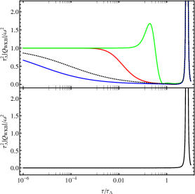
Figure 3: Top panel: WKB approximation in BI universes. Continuous lines show the quantity $|Q_{{\rm WKB}}|/\omega^{2}$ as a function of time for a mode $k=5\tau^{-1}_{\Lambda}$ aligned with the $x$, $y$ and $z$ axes (red, green and blue, respectively) and for $\alpha=\pi/4$. The dotted line shows a mode with the same modulus distributed equally over the three directions. Note that the approximation is good after $\tau\geq\tau_{\Lambda}$, when the shear has decayed. The bottom panel shows the same quantity for a FL universe, and using the same Fourier mode. Here, the approximation works throughout the entire past, and the adiabatic vacuum prescription fixes the amplitude unambiguously.

III.2 Perturbations generalities

The last section focused on the evolution of a test field in an unperturbed background. The inclusion of linear matter perturbations coupled to the perturbations of the metric leads to additional complications Pitrou:2008gk , but also to potentially new observational features. During inflation, these perturbations are described by three canonical variables, one describing the scalar perturbations, $v$, and two representing the polarizations of the gravitational waves, $\mu_{+}$ and $\mu_{\times}$. These variables can be arranged in a three-dimensional vector

$$\mathbf{V}=(v(\mathbf{k},\tau),\mu_{+}(\mathbf{k},\tau),\mu_{\times}(\mathbf{k},\tau))\,,$$

whose dynamics is described, in Fourier space, by the following action Pereira:2007yy

$$S=\frac{M_{p}^{2}}{2}\int{\rm d}t{\rm d}^{3}k\left(|V^{\prime}|^{2}-k^{2}|V|^{2}+\mathbf{V}^{\dagger}\cdot\mathbf{M}\cdot\mathbf{V}\right)$$

where $\mathbf{M}$ is an hermitian and non-diagonal matrix which depends on the time, the Fourier mode $\mathbf{k}$ and the components of the shear in a given basis. Note that the vector perturbations do not appear in the action. However, they can no longer be neglected, since they appear as constraints relating scalar and tensor modes, and it is crucial to consider them in intermediary steps when determining the form of the action Pereira:2007yy .

When varied, this action leads to

$$\mathbf{V}^{\prime\prime}+k^{2}\mathbf{V}=\mathbf{M}\cdot\mathbf{V}\,.$$ (29)

It is the equation ruling the evolution of three harmonic equations (one for the scalar mode and two for the tensor modes) coupled by the matrix $\mathbf{M}$. These couplings are most important at large scales, and decay at sufficiently small scales, as one might expect from the local isotropy of the spacetime. Their general effect is twofold: first, since each gravity wave polarization has its own dynamics, their primordial power spectra will also differ, mostly at the horizon scale. Second, in the presence of the matrix $\mathbf{M}$ the variables $v$, $\mu_{+}$ and $\mu_{\times}$ are no longer statistically independent , even if they are defined independently at $\tau=0$. In particular, this implies that the matter correlation at large scales will share power with the correlation of gravitational waves, and vice-versa. Nonetheless, the effect of these cross-correlations is expected to be small, and in a first analysis we can focus on their individual (self-correlation) power spectra:

$${\cal P}_{X}(\mathbf{k})=f_{X}(k)\left[1+\sum_{\ell,m}r^{X}_{\ell m}(k)Y_{\ell m}(\hat{\mathbf{k}})\right]$$ (30)

where $X$ stands for either $v$, $\mu_{+}$ and $\mu_{\times}$. Here, $f_{X}(k)$ is the monopole of the expansion, and represents the isotropic power spectrum. The coefficients $r^{X}_{\ell m}(k)$ characterize the deviation from isotropy, and for this reason they tend to vanish for $\ell\gg 1$ and $k\gg SH|_{\tau_{\Lambda}}$, where $\tau_{\Lambda}$ is the isotropization time. Furthermore, there are restrictions on the multipoles $r^{X}_{\ell m}(k)$ as we discuss below, and it can have important consequences for the issue of CMB anomalies.

III.3 Relation to CMB statistical anomalies

Since the assumed isotropy of the universe is one of the central hypotheses of the standard cosmological model, local tests of spatial isotropy are a fundamental problem on its own uzan2010dark . Nonetheless, further motivation to conduct these tests come from large angle features of CMB, which suggest that new physics could be lurking at the horizon scale. Such features are known as statistical anomalies, and were initially reported by several independent groups using WMAP data Bennett:2010jb ; deOliveiraCosta:2003pu ; Schwarz:2004gk ; Eriksen:2003db ; Land:2005ad . The robustness of these anomalies have gained strength after the release of the Planck data Ade:2013nlj ; Ade:2015hxq , since several of the initial WMAP anomalies have survived the completely different pipeline analysis of the Planck collaboration Copi:2013cya ; Copi:2013jna ; Bernui:2014gla ; Akrami:2014eta (see Copi:2010na for a comprehensive review). Since their initial report, several models in which isotropy is explicitly violated have been offered as possible mechanism for the reported anomalies Jaffe:2005gu ; Campanelli:2006vb ; Boehmer:2007ut ; Rodrigues:2007ny . It is thus interesting to ask what are the generic consequences of anisotropic models to the spectrum of CMB at large scales. To be more specific, let us consider the case of homogeneous but anisotropic models, such as those resulting from anisotropic Bianchi metrics.

Let ${\cal O}_{\mathbf{k}}(\tau)$ be one realization of a (Fourier transformed) Gaussian random cosmological observable. In a spatially homogeneous but anisotropic spacetime, its ensemble average at a fixed time obeys

$$\langle{\cal O}_{\mathbf{k}}\overline{{\cal O}}_{\mathbf{q}}\rangle=P(\mathbf{k})\delta^{(3)}(\mathbf{k}-\mathbf{q})\,,$$ (31)

where we have dropped the time dependence for simplicity and the overbar denotes complex conjugation. Note that the statistical independence of the scales imposed by the delta function is a direct consequence of spatial homogeneity. Spatial anisotropy further demands the power spectrum $P$ to be a function of the full vector $\mathbf{k}$. From the definition (31) and the properties of the delta function, we also find

$$\langle\overline{{\cal O}_{\mathbf{k}}\overline{{\cal O}}_{\mathbf{q}}}\rangle =\langle\overline{{\cal O}}_{\mathbf{k}}{\cal O}_{\mathbf{q}}\rangle$$

$$=P(\mathbf{q})\delta^{(3)}(\mathbf{q}-\mathbf{k})$$

$$=P(\mathbf{k})\delta^{(3)}(\mathbf{k}-\mathbf{q})$$

$$=\langle{\cal O}_{\mathbf{k}}\overline{{\cal O}}_{\mathbf{q}}\rangle\,,$$

which shows that $P(\mathbf{k})$ is real. It implies the restriction $\bar{r}^{X}_{\ell m}(k)=(-1)^{m}r^{X}_{\ell\,-m}(k)$ on Eq. (30). Furthermore, using the reality condition ${\cal O}_{\mathbf{k}}={\overline{\cal O}}_{-\mathbf{k}}$ together with the last result, we find

$$\langle{\cal O}_{\mathbf{k}}\overline{{\cal O}}_{\mathbf{q}}\rangle =\langle\overline{{\cal O}}_{\mathbf{k}}{\cal O}_{\mathbf{q}}\rangle\,$$

$$=\langle{\cal O}_{-\mathbf{k}}\overline{{\cal O}}_{-\mathbf{q}}\rangle\,$$

$$=P(-\mathbf{k})\delta^{(3)}(\mathbf{k}-\mathbf{q})\,,$$

which shows that

$$P(\mathbf{k})=P(-\mathbf{k})\,.$$ (32)

Apart from the assumption of null vorticity of the spacetime Sundell:2015gra , this result is quite general, and tells us that homogeneous but anisotropic models respect parity. It implies that any $r^{X}_{\ell m}(k)$ vanishes when with an odd $\ell$. Interestingly, some of the reported CMB anomalies look like a genuine violation of parity. This is the case, for example, of the quadrupole-octopole alignment Land:2005ad , which suggests a temperature covariance matrix of the form $\langle a_{2m}\overline{a}_{3m}\rangle$. However, at large scales, the radiation transfer starting from initial conditions whose power spectrum respects Eq. (32) can only produce even-even and odd-odd correlations Abramo:2010gk ; Pullen:2007tu . Another example is the observed north-south asymmetry in the CMB maps, which is usually modelled with a power spectrum of the form $P(\mathbf{k})=P(k)(1+A\hat{\mathbf{k}}\cdot\hat{\mathbf{z}}$), where $A$ is an overall amplitude and $\hat{\mathbf{z}}$ is the direction of the north-south asymmetry Dai:2013kfa ; Mazumdar:2013yta . Clearly, this form violates (32), and thus it cannot result from anisotropy alone.

We thus conclude that, if parity-violating CMB anomalies are indeed a result of new physics, these are more likely to result from a break of translation invariance, either explicitly Carroll:2008br , or as a consequence of mode-coupling induced by non-gaussian statistics Schmidt:2012ky ; Schmidt:2010gw .

IV Alternative models

In § II.1, we have shown that slow-roll inflation classically erases primordial anisotropies, so that any initial shear, no matter how large, is quickly diluted by the expansion. However, since the details of inflation are still elusive, it is important to point the existence of alternative models which could circumvent this fact.

IV.1 Vector inflation

The lack of primordial “anisotropic hair” is a generic feature of Bianchi models in the presence of a cosmological constant, and is known as the cosmic no-hair theorem Wald:1983ky . However, this theorem can be easily violated if the spacetime is endowed with extra anisotropic degrees of freedom. In recent years, several works have addressed the dynamics of inflation in the presence of vector fields Watanabe:2009ct ; Yokoyama:2008xw ; Ford:1989me ; Golovnev:2008cf ; Koivisto:2008xf . The main idea behind these models is to preserve some of the primordial anisotropy during inflation, so as to potentially produce classical signatures at CMB.

One of the earliest attempts to inflate the universe with a vector field was conducted in Ford:1989me , although the primary motivation was to solve initial condition problems rather than understanding classical anisotropies. In this model, a minimally and self-coupled vector theory of the form

$${\cal L}=-\frac{M^{2}_{p}}{4}F_{\mu\nu}F^{\mu\nu}+V\left(A_{\lambda}A^{\lambda}\right)$$ (33)

was used to produce inflation. If the potential $V$ is sufficiently flat, then expansion is almost de Sitter, but the final signature is anisotropic due to the presence of a preferred direction in the energy momentum tensor. In 2008, Ref. Golovnev:2008cf extended this idea to the case of $N$ randomly oriented and non-minimally coupled vector fields, where it was found that inflation can lead to reminiscent anisotropies of order $1/\sqrt{N}$. Unfortunately, vector field models of these types are plagued with instabilities EspositoFarese:2009aj , and their validity as cosmological models is still an ongoing debate.

If vector fields are not the driving source of inflation, they could at least play a role as spectator fields. One explicit example arises in the context of supergravity inspired models Martin:2007ue , where the expansion is still driven by a canonical scalar field $\varphi$, but this time with a vector field coupled to the inflaton by means of a free function $f$

$${\cal L}\supset-\frac{1}{4}f(\varphi)^{2}F_{\mu\nu}F^{\mu\nu}\,.$$ (34)

In the context of anisotropic inflation, this idea was explored in Watanabe:2009ct . It was found that, for a large class of the coupling function $f$, inflation goes through two slow-roll regimes. Due to the presence of the vector field, the ratio $\dot{\beta}/H$ grows during the first slow-roll phase, saturating at values of order a few percent. Indeed, the dynamics of the system possesses a tracking solution where the vector field energy density follows that of the inflaton during the first slow-roll stage, and remaining nearly constant in the second stage. One can then show that, during the second slow-roll phase, the amplitude of the shear scales as

$$\frac{\sigma}{H}\approx\frac{1}{3}\varepsilon\,,$$ (35)

where $\varepsilon\equiv-\dot{H}/H^{2}$ is the slow-roll parameter. Interestingly, this model completely determines the amplitude of the shear in terms of the slow-roll parameter. Since the latter is of the order of a few percent, the effect of a primordial anisotropy could be bordering on current error bars of CMB temperature spectrum. Moreover, since the spacetime is anisotropic, the model also predicts an anisotropic power spectrum in accordance with the discussion of last section. More importantly, this model is free from instabilities Fleury:2014qfa , offering thus an interesting possibility to test the stages of the universe prior to inflation.

IV.2 Shear-free inflation

In all the models discussed so far, the anisotropy manifests itself through the spatial shear. However, once we are willing to give up rotational invariance, we learn that anisotropic expansion is just one possibility. Indeed, we can imagine models where the expansion is isotropic (i.e., $\sigma_{ij}=0$), but the curvature of the spatial sections is not. These models are known as shear-free cosmologies Mimoso:1993ym ; Abebe:2015ega .

The simplest examples of shear-free cosmologies are realized with the Bianchi III (BIII) and Kantowski-Sachs (KS) metrics, which have spatial sections of the form $\mathbb{H}^{2}\times\mathbb{R}$ and $\mathbb{S}^{2}\times\mathbb{R}$, respectively. Evidently, the anisotropy of the spatial sections can only be maintained at the cost of an imperfect energy-momentum tensor Barrow:1997sy ; Barrow:1998ih . However, the shear-free condition strongly constrain its form. Consider for example the evolution equation for the shear in 1+3 formalism ellis2012relativistic

$$\dot{\sigma}_{\mu\nu}+\sigma_{\mu}^{\,\alpha}\sigma_{\alpha\nu}+\frac{2}{3}\theta\sigma_{\mu\nu}-\frac{2}{3}\sigma^{2}h_{\mu\nu}-\frac{1}{2}\pi_{\mu\nu}+E_{\mu\nu}=0$$

where $\theta$ is the expansion scalar, $h_{\mu\nu}$ is the (covariant) spatial metric, $\pi_{\mu\nu}$ the matter anisotropic stress and $E_{\mu\nu}$ is the electric part of the Weyl tensor. Clearly, the condition $\sigma_{\mu\nu}=0$ leads to $\pi_{\mu\nu}=2E_{\mu\nu}$. The remarkable consequence of this choice is that, for the BIII and KS metrics, the background equations are formally the Friedmann equations with spatial curvature Mimoso:1993ym ; Carneiro:2001fz . Thus, at the background level, slow-roll inflation will proceed exactly as in a FL universe, and the spatial anisotropy will be diluted as $1/S^{2}$, as usual. In other words, the observational signatures of these models lie entirely in the perturbed sector Pereira:2012ma , and thus in the form of the primordial power spectrum.

Shear-free cosmologies have important properties which render them viable cosmological models. First, one can check that the choice $\pi_{\mu\nu}=2E_{\mu\nu}$ is a dynamically stable fixed point of the background equations. Moreover, during inflation, the equation governing the perturbations $\delta\pi_{\mu\nu}$ of the stress tensor has only decaying modes, so that one can make definite predictions for the perturbed quantities without worrying with the phenomenological model producing such an anisotropic stress Pereira:2015pxa .

The theory of linear perturbations in shear-free cosmologies share similarities with both perturbed theories in FL and BI universes. Since there is only one scale factor, perturbative modes do not couple dynamically during inflation Pereira:2012ma , and the perturbed equations for the scalar degree of freedom is formally identical to the one in FL universes. On the other hand, the two tensor degrees of freedom have independent dynamics, so one expect non-trivial signatures from gravitational waves. One important difference in shear-free cosmologies result from the eigenfunctions of the spatial Laplacian. Due to the presence of spatial curvature, the wavelengths of perturbations have an upper limit given by the curvature radius. The existence of such limit leads to interesting observational signatures, such as the existence of supercurvature perturbations Lyth:1995cw , and their possible effects on CMB through the Grishchuk - Zeldovich effect GarciaBellido:1995wz .

V Final words

The fact that inflation is the only viable model for the origin of large-scale structures forces us to test its robustness against all sorts of extensions. In this review we have explored extensions of slow-roll inflation that accommodate a pre-inflationary anisotropic phase. The effect of inflation is to quickly erase classical inhomogeneities, although early signatures can survive in the spectrum of primordial quantum fluctuations. Unfortunately, the lack of rotational symmetry makes it impossible to define an adiabatic vacuum throughout the anisotropic era. Thus, definite predictions can only be trusted for modes sourced at the onset of inflation, when the shear is nearly zero, but where the WKB approximation is still valid. Furthermore, if the number of e-folds exceeds the minimum required to solve cosmological problems, no observational signatures from a pre-inflationary anisotropic phase would be left.

On the other hand, it should be noted that the above description corresponds to a frugal inflationary model, i.e., single field inflation plus general relativity. In fact, the prediction of anisotropic hair can be achieved if one invokes extra degrees of freedom. Although pure vector field models are generally plagued with instabilities, one can devise stable models in which the vector field is coupled to the inflaton, such as happens in supergravity inspired models. In this case, and for a large class of coupling functions, the primordial shear survives slow-roll inflation, converging to a final value of the order of slow-roll parameters, and thus potentially detectable in CMB maps.

Another possibility of testing pre-inflationary physics is offered by shear-free cosmological models, where the expansion of the universe is isotropic, but spatial curvature is direction dependent. Such models represent an explicit demonstration that the observed symmetry of CMB does not imply an equally symmetric background, and remind us of the possible perils with standard symmetry assumptions. Observationally, shear-free models can be tested by the detection of supercurvature perturbations, as well as a non-trivial dynamics of gravitational waves.

Finally, we have demonstrated that anisotropic cosmological models without vorticity respect parity, as long as spatial homogeneity persists. Thus, since most of the CMB anomalies point to a break of parity – and assuming that they are indeed physical – they cannot result from a break of rotational symmetry alone. This suggest that inhomogeneous cosmological models are more likely to explain the existing anomalies.

- (1) A. H. Guth, Phys. Rev. D23, 347 (1981).
- (2) A. D. Linde, Lect. Notes Phys. 738, 1 (2008), [0705.0164].
- (3) C. L. Bennett et al., Astrophys. J. Suppl. 192, 17 (2011), [1001.4758].
- (4) Planck, P. A. R. Ade et al., Astron. Astrophys. 571, A23 (2014), [1303.5083].
- (5) Planck, P. A. R. Ade et al., 1506.07135.
- (6) D. S. Goldwirth, Phys. Rev. D43, 3204 (1991).
- (7) N. Deruelle and D. S. Goldwirth, Phys. Rev. D51, 1563 (1995), [gr-qc/9409056].
- (8) C. Pitrou, T. S. Pereira and J.-P. Uzan, JCAP 0804, 004 (2008), [0801.3596].
- (9) I. Moss and V. Sahni, Phys. Lett. B178, 159 (1986).
- (10) L. Kofman, J.-P. Uzan and C. Pitrou, JCAP 1105, 011 (2011), [1102.3071].
- (11) A. D. Linde, Phys. Lett. B129, 177 (1983).
- (12) P. Peter and J.-P. Uzan, Primordial cosmology (Oxford University Press, 2013).
- (13) A. E. Gumrukcuoglu, C. R. Contaldi and M. Peloso, JCAP 0711, 005 (2007), [0707.4179].
- (14) T. S. Pereira, C. Pitrou and J.-P. Uzan, JCAP 0709, 006 (2007), [0707.0736].
- (15) V. F. Mukhanov, H. A. Feldman and R. H. Brandenberger, Phys. Rept. 215, 203 (1992).
- (16) A. E. Gumrukcuoglu, B. Himmetoglu and M. Peloso, Phys. Rev. D81, 063528 (2010), [1001.4088].
- (17) T. S. Pereira, C. Pitrou and J.-P. Uzan, 1503.01127.
- (18) C. Pitrou, T. S. Pereira and J.-P. Uzan, Phys. Rev. D92, 023501 (2015), [1503.01125].
- (19) J. Martin and D. J. Schwarz, Phys. Rev. D67, 083512 (2003), [astro-ph/0210090].
- (20) J.-P. Uzan, Dark energy: observational and theoretical approaches (2010).
- (21) A. de Oliveira-Costa, M. Tegmark, M. Zaldarriaga and A. Hamilton, Phys. Rev. D69, 063516 (2004), [astro-ph/0307282].
- (22) D. J. Schwarz, G. D. Starkman, D. Huterer and C. J. Copi, Phys. Rev. Lett. 93, 221301 (2004), [astro-ph/0403353].
- (23) H. K. Eriksen, F. K. Hansen, A. J. Banday, K. M. Gorski and P. B. Lilje, Astrophys. J. 605, 14 (2004), [astro-ph/0307507], [Erratum: Astrophys. J.609,1198(2004)].
- (24) K. Land and J. Magueijo, Phys. Rev. Lett. 95, 071301 (2005), [astro-ph/0502237].
- (25) C. J. Copi, D. Huterer, D. J. Schwarz and G. D. Starkman, 1310.3831.
- (26) C. J. Copi, D. Huterer, D. J. Schwarz and G. D. Starkman, Mon. Not. Roy. Astron. Soc. 449, 3458 (2015), [1311.4562].
- (27) A. Bernui, A. F. Oliveira and T. S. Pereira, JCAP 1410, 041 (2014), [1404.2936].
- (28) Y. Akrami et al., Astrophys. J. 784, L42 (2014), [1402.0870].
- (29) C. J. Copi, D. Huterer, D. J. Schwarz and G. D. Starkman, Adv. Astron. 2010, 847541 (2010), [1004.5602].
- (30) T. R. Jaffe, S. Hervik, A. J. Banday and K. M. Gorski, Astrophys. J. 644, 701 (2006), [astro-ph/0512433].
- (31) L. Campanelli, P. Cea and L. Tedesco, Phys. Rev. Lett. 97, 131302 (2006), [astro-ph/0606266], [Erratum: Phys. Rev. Lett.97,209903(2006)].
- (32) C. G. Boehmer and D. F. Mota, Phys. Lett. B663, 168 (2008), [0710.2003].
- (33) D. C. Rodrigues, Phys. Rev. D77, 023534 (2008), [0708.1168].
- (34) P. Sundell and T. Koivisto, [arXiv:1506.04715].
- (35) L. R. Abramo and T. S. Pereira, Adv. Astron. 2010, 378203 (2010), [1002.3173].
- (36) A. R. Pullen and M. Kamionkowski, Phys. Rev. D76, 103529 (2007), [0709.1144].
- (37) L. Dai, D. Jeong, M. Kamionkowski and J. Chluba, Phys. Rev. D87, 123005 (2013), [1303.6949].
- (38) A. Mazumdar and L. Wang, JCAP 1310, 049 (2013), [1306.5736].
- (39) S. M. Carroll, C.-Y. Tseng and M. B. Wise, Phys. Rev. D81, 083501 (2010), [0811.1086].
- (40) F. Schmidt and L. Hui, Phys. Rev. Lett. 110, 011301 (2013), [1210.2965], [Erratum: Phys. Rev. Lett.110,059902(2013)].
- (41) F. Schmidt and M. Kamionkowski, Phys. Rev. D82, 103002 (2010), [1008.0638].
- (42) R. M. Wald, Phys. Rev. D28, 2118 (1983).
- (43) M.-a. Watanabe, S. Kanno and J. Soda, Phys. Rev. Lett. 102, 191302 (2009), [0902.2833].
- (44) S. Yokoyama and J. Soda, JCAP 0808, 005 (2008), [0805.4265].
- (45) L. H. Ford, Phys. Rev. D40, 967 (1989).
- (46) A. Golovnev, V. Mukhanov and V. Vanchurin, JCAP 0806, 009 (2008), [0802.2068].
- (47) T. Koivisto and D. F. Mota, JCAP 0808, 021 (2008), [0805.4229].
- (48) G. Esposito-Farese, C. Pitrou and J.-P. Uzan, Phys. Rev. D81, 063519 (2010), [0912.0481].
- (49) J. Martin and J. Yokoyama, JCAP 0801, 025 (2008), [0711.4307].
- (50) P. Fleury, J. P. B. Almeida, C. Pitrou and J.-P. Uzan, JCAP 1411, 043 (2014), [1406.6254].
- (51) J. P. Mimoso and P. Crawford, Class. Quant. Grav. 10, 315 (1993).
- (52) A. Abebe, D. Momeni and R. Myrzakulov, 1507.03265.
- (53) J. D. Barrow, Phys. Rev. D55, 7451 (1997), [gr-qc/9701038].
- (54) J. D. Barrow and R. Maartens, Phys. Rev. D59, 043502 (1999), [astro-ph/9808268].
- (55) G. F. Ellis, R. Maartens and M. A. MacCallum, Relativistic cosmology (Cambridge University Press, 2012).
- (56) S. Carneiro and G. A. Mena Marugan, Phys. Rev. D64, 083502 (2001), [gr-qc/0109039].
- (57) T. S. Pereira, S. Carneiro and G. A. M. Marugan, JCAP 1205, 040 (2012), [1203.2072].
- (58) T. S. Pereira, G. A. M. Marugán and S. Carneiro, JCAP 1507, 029 (2015), [1505.00794].
- (59) D. H. Lyth and A. Woszczyna, Phys. Rev. D52, 3338 (1995), [astro-ph/9501044].
- (60) J. Garcia-Bellido, A. R. Liddle, D. H. Lyth and D. Wands, Phys. Rev. D52, 6750 (1995), [astro-ph/9508003].