The Lyapunov dimension and its computation for self-excited and hidden attractors in the Glukhovsky-Dolzhansky fluid convection model

Abstract

Consideration of various hydrodynamic phenomena involves the study of the Navier-Stokes (N-S) equations, what is hard enough for analytical and numerical investigations since already in three-dimensional (3D) case it is a challenging task to study the limit behavior of N-S solutions. The low-order models (LOMs) derived from the initial N-S equations by Galerkin method allow one to overcome difficulties in studying the limit behavior and existence of attractors. Among the simple LOMs with chaotic attractors there are famous Lorenz system, which is an approximate model of two-dimensional convective flow and Glukhovsky-Dolzhansky model, which describes a convective process in three-dimensional rotating fluid and can be considered as an approximate model of the World Ocean. One of the widely used dimensional characteristics of attractors is the Lyapunov dimension. In the study we follow a rigorous approach for the definition of the Lyapunov dimension and justification of its computation by the Kaplan-Yorke formula, without using statistical physics assumptions. The exact Lyapunov dimension formula for the global attractors is obtained and peculiarities of the Lyapunov dimension estimation for self-excited and hidden attractors are discussed. A tutorial on numerical estimation of the Lyapunov dimension on the example of the Glukhovsky-Dolzhansky model is presented.

1 Introduction

The main difficulties in studying fluid motion are related to infinite number of degrees of freedom of hydrodynamic objects. To overcome these difficulties, one may use an approximation (e.g., applying Galerkin method [1]) of system of equations, describing the considered object with an infinite number of degrees of freedom, by a system of equations with a finite number of degrees of freedom. Resulting finite-dimensional analogues of the hydrodynamic equations, called low-order models, turn out to be more convenient for analytical and numerical investigations [2, 3, 4]. Among the famous physically sounded low-order models there are the Lorenz model [5] (describing the Rayleigh-Bénard convection), the Vallis model [6] (describing El Niño climate phenomenon), and the Glukhovsky-Dolzhansky model [7] (describing fluid convection inside the rotating ellipsoidal cavity under the horizontal heating). One of the substantial features of these models is the existence of chaotic attractors in their phase spaces. From both theoretical and practical perspective it is important to localize these attractors [8, 9], study their basins of attraction [10, 11, 12], and estimate their dimensions [13] with respect to varying parameters.

In the present paper a there-dimensional model, describing the convection of fluid within an ellipsoidal rotating cavity under an external horizontal heating, is considered. This model was suggested by Glukhovsky and Dolghansky [7] (G-D) and can be considered as an approximate model of the World Ocean. The mathematical G-D model is described by the following system of ODEs:

$$\begin{array}[]{l}\dot{x}=-\sigma x+z+a_{0}yz,\\ \dot{y}=R-y-xz,\\ \dot{z}=-z+xy,\end{array}$$ (1)

where $\sigma$, $R$, $a_{0}$ are positive parameters.

After the change of variables:

$$(x,\,y,\,z)\quad\rightarrow\quad\left(x,\,R-\frac{\sigma}{a_{0}R+1}z,\,\frac{\sigma}{a_{0}R+1}y\right),$$ (2)

system (1) takes the form of generalized Lorenz system

$$\begin{array}[]{l}\dot{x}$ = $-\sigma x+\sigma y-Ayz,\\ \dot{y}$ = $rx-y-xz,\\ \dot{z}$ = $-bz+xy,\end{array}$$ (3)

where

$$b=1,\quad A=\frac{a_{0}\sigma^{2}}{(a_{0}R+1)^{2}},\quad r=\frac{R}{\sigma}(a_{0}R+1).$$ (4)

If

$$R=r(\sigma-Ar)>0,\quad a_{0}=\frac{A}{(\sigma-Ar)^{2}}>0,\quad b=1.$$ (5)

then we have the inverse transformation

$$(x,\,y,\,z)\to\left(x,\,\frac{1}{\sigma-Ar}\,z,\,r-\frac{1}{\sigma-Ar}\,y\right).$$

For $A=0$ system (3) coincides with the classical Lorenz system [5].

System (3) with the parameters $r$, $\sigma$, $b>0$ is mentioned first in the work of Rabinovich [14] and in the case $A<0$ can be transformed [15] to the Rabinovich system of waves interaction in plasma [16, 17]. Following Glukhovsky and Dolghansky [7], consider system (3) under the physically sounded assumption that $r$, $\sigma$, $b$, $A$ are positive.

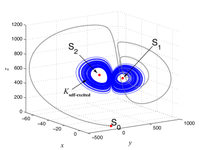
(a) Monostability ($r=687.5$): trajectories from almost all initial points except for a set of zero measure (including unstable equilibria $S_{0,1,2}$) tend to the same chaotic attractor $K_{\text{self-excited}}$ (self-excited attractor with respect to all three equilibria: e.g. one-dimensional unstable manifold of $S_{0}$ is attracted to $K_{\text{self-excited}}$ and, thus, visualizes it).

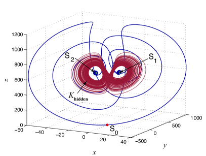
(b) Multistability ($r=700$): Coexistence of three local attractors — two stable equilibria $S_{1,2}$ and one chaotic attractor $K_{\text{hidden}}$ (hidden attractor, which basin of attraction does not overlap with an arbitrarily small vicinity of equilibria: one-dimensional unstable manifold of $S_{0}$ is attracted to $S_{1,2}$).

Figure 1: Self-excited and hidden attractors in system (3) with $b=1$, $\sigma=4$, $A=0.0052$.

Systems (1) and (3) are of particular interest because they have chaotic attractors (Fig. 1). By numerical simulations in the case when parameter $\sigma=4$ it is obtained [7] certain values of the parameters for which systems (1) and (3) possess self-excited attractors (Fig. 1a). An attractor is called a self-excited attractor if its basin of attraction intersects an arbitrarily small open neighborhood of an equilibrium, otherwise it is called a hidden attractor [18, 19, 20, 21]. Self-excited attractors are relatively simple for localization and can be obtained using trajectories from an arbitrary small neighborhood of unstable equilibrium. The use of the term self-excited oscillation or self-oscillations can be traced back to the works of H.G. Barkhausen and A.A. Andronov, where it describes the generation and maintenance of a periodic motion in mechanical and electrical models by a source of power that lacks any corresponding periodicity (e.g., stable limit cycle in the van der Pol oscillator) [22, 23]. We use this notion for attractors of dynamical systems to describe the existence of transient process from a small vicinity of an unstable equilibrium to an attractor. If there is no such a transient process for an attractor, it is called a hidden attractor. The hidden and self-excited classification of attractors was introduced by Leonov and Kuznetsov in connection with the discovery of hidden Chua attractor [24, 18, 25] and its rigorous consideration for autonomous and nonautonomous systems can be found in [20, 21, 26, 12]. For example, hidden attractors are attractors in systems without equilibria or with only one stable equilibrium (a special case of multistability and coexistence of attractors). Some examples of hidden attractors can be found in [27, 28, 29, 30, 31, 32, 33, 34, 35, 36, 37, 38, 39, 40, 12]. Recently hidden attractors were localized [41, 21] in systems (1) and (3) (Fig. 1b).

By the Lyapunov function $V(x,y,z)=\frac{1}{2}\left(x^{2}+y^{2}+(A+1)\left(z-\frac{\sigma+r}{A+1}\right)^{2}\right)$ it is proved [15] that system (3) possesses a bounded absorbing ellipsoid (thus it is dissipative in the sense of Levinson [21])

$$\mathcal{B}(r,\sigma,A)=\left\{(x,y,z)\in\mathbb{R}^{3}~{}|~{}V(x,y,z)\leq\frac{(\sigma+r)^{2}}{2(A+1)}\right\}$$ (6)

and, thus, has a global attractor and generates a dynamical system. Also it is known [15] that for $b=1$ the global attractor is located in the positive invariant set

$$\Omega=\left\{y^{2}+z^{2}\leq 2rz\right\}.$$ (7)

To obtain necessary conditions of the existence of self-excited attractor, we consider the stability of equilibria in system (3). According to [15], we have the following: if $r<1$, then there is a unique equilibrium ${\bf\rm S_{0}}=(0,\,0,\,0)$ (the trivial case). If $r>1$, then (3) has three equilibria: ${\bf\rm S_{0}}=(0,\,0,\,0)$ – saddle, and ${\bf\rm S_{1,2}}=(\pm x_{1},\,\pm y_{1},\,z_{1})$, where

$$x_{1}=\frac{\sigma b\sqrt{\xi}}{\sigma b+A\xi},\quad y_{1}=\sqrt{\xi},\quad z_{1}=\frac{\sigma\xi}{\sigma b+A\xi},\quad\xi=\frac{\sigma b}{2A^{2}}\left[A(r-2)-\sigma+\sqrt{(Ar-\sigma)^{2}+4A\sigma}\right].$$

The stability of $S_{1,2}$ depends on the parameters, e.g. for $b=1$, $\sigma=4$ the stability domain [21] is shown in Fig. 2. Here for parameters from the non-shaded region, a self-excited attractor can be localized by a trajectory from a small neighborhood of $S_{0}$, $S_{1}$ or $S_{2}$.

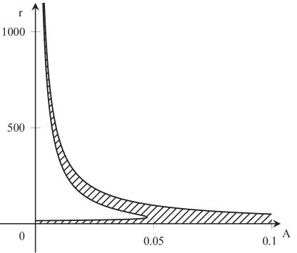
Figure 2: Stability domain (shaded) of the equilibria $S_{1,2}$ for $b=1$, $\sigma=4$.

To get a numerical characteristic of chaos in a system using numerical methods, it is possible to compute a local Lyapunov dimension for this trajectory, what gives an estimation of Lyapunov dimension of the corresponding self-excited attractor. For the hidden attractor visualization in the considered systems we need to use special analytical-numerical procedures of searching for a point in its domain of attraction [41, 21]. Thus, the estimation of Lyapunov dimension of hidden attractors in the considered systems is a challenging task.

2 Preliminaries. Analytical estimates of the Lyapunov dimension

2.1 The Lyapunov dimension and Kaplan-Yorke formula

The concept of the Lyapunov dimension was suggested in the seminal paper by Kaplan and Yorke [42] for estimating the Hausdorff dimension of attractors. Later it has been developed and rigorously justified in a number of papers (see, e.g. [43, 44, 45] and others). The direct numerical computation of the Hausdorff dimension of chaotic attractors is often a problem of high numerical complexity (see, e.g. the discussion in [46]), thus, the estimates by the Lyapunov dimension are of interest (see, e.g. [13]). Along with numerical methods for computing the Lyapunov dimension there is an effective analytical approach, proposed by Leonov in 1991 [47] (see also [15, 48, 49]). The Leonov method is based on a combination of the Douady-Oesterlé approach with the direct Lyapunov method. The advantage of the method is that it often allows one to estimate the Lyapunov dimension of attractor without localization of attractor in the phase space and, in many cases, to get an exact Lyapunov dimension formula [50, 51, 52, 53, 54, 55, 56].

Nowadays it is known various approaches to the definition of the Lyapunov dimension. Below we use a rigorous definition [49] of the Lyapunov dimension inspirited by the Douady-Oesterlé theorem on the Hausdorff dimension of maps. Consider an autonomous differential equation

$$\dot{u}=f(u),$$ (8)

where $f:U\subseteq\mathbb{R}^{n}\to\mathbb{R}^{n}$ is a continuously differentiable vector-function, $U$ is an open set. Define by $u(t,u_{0})$ a solution of (8) such that $u(0,u_{0})=u_{0}$, and consider the evolutionary operator $\varphi^{t}(u_{0})=u(t,u_{0})$. We assume the uniqueness and existence of solutions of (8) for $t\in[0,+\infty)$. Then system (8) generates a dynamical system $\{\varphi^{t}\}_{t\geq 0}$. Let a nonempty set $K\subset U$ be invariant with respect to $\{\varphi^{t}\}_{t\geq 0}$, i.e. $\varphi^{t}(K)=K$ for all $t\geq 0$. Consider the linearization of system (8) along the solution $\varphi^{t}(u)$:

$$\dot{v}=J(\varphi^{t}(u))v,\quad J(u)=Df(u),$$ (9)

where $J(u)$ is the $n\times n$ Jacobian matrix, the elements of which are continuous functions of $u$. Suppose that $\det J(u)\neq 0\quad\forall u\in U$. Consider a fundamental matrix of linearized system (9) $D\varphi^{t}(u)$ such that $D\varphi^{0}(u)=I$, where $I$ is a unit $n\times n$ matrix. Let $\sigma_{i}(t,u)=\sigma_{i}(D\varphi^{t}(u))$, $i=1,2,..\,n$, be the singular values of $D\varphi^{t}(u)$ with respect to their algebraic multiplicity ordered so that $\sigma_{1}(t,u)\geq...\geq\sigma_{n}(t,u)>0$ for any $u\in U$ and $t\geq 0$. The singular value function of order $d\in[0,n]$ at $u\in U$ is defined as

$$\begin{cases}\omega_{0}(D\varphi^{t}(u))=1,\\ \omega_{d}(D\varphi^{t}(u))=\sigma_{1}(t,u)\cdots\sigma_{\lfloor d\rfloor}(t,u)\sigma_{\lfloor d\rfloor+1}(t,u)^{d-\lfloor d\rfloor},\ \quad d\in(0,n),\\ \omega_{n}(D\varphi^{t}(u))=\sigma_{1}(t,u)\cdots\sigma_{n}(t,u),\\ \end{cases}$$ (10)

where ${\lfloor d\rfloor}$ is the largest integer less or equal to $d$. For a certain moment of time $t$ the local Lyapunov dimension of the map $\varphi^{t}$ at the point $u\in\mathbb{R}^{n}$ (or the finite-time local Lyapunov dimension of dynamical system $\{\varphi^{t}\}_{t\geq 0}$) is defined as [49]

$$\dim_{\rm L}(\varphi^{t},u)=\max\{d\in[0,n]:\omega_{d}(D\varphi^{t}(u))\geq 1\}$$ (11)

and the Lyapunov dimension of the map $\varphi^{t}$ (or the finite-time Lyapunov dimension of dynamical system $\{\varphi^{t}\}_{t\geq 0}$) with respect to invariant set $K$ is defined as

$$\dim_{\rm L}(\varphi^{t},K)=\sup\limits_{u\in K}\dim_{\rm L}(\varphi^{t},u)=\sup\limits_{u\in K}\max\{d\in[0,n]:\omega_{d}(D\varphi^{t}(u))\geq 1\}.$$ (12)

The following is a corollary of the fundamental Douady–Oesterlé theorem [43]

Theorem 1.

For any fixed $t>0$ the Lyapunov dimension of the map $\varphi^{t}$ with respect to a compact invariant set $K$, defined by (12), is an upper estimate of the Hausdorff dimension of the set $K$: $\dim_{\rm H}K\leq\dim_{\rm L}(\varphi^{t},K)$.

For the estimation of the Hausdorff dimension of invariant compact set $K$ one can use the map $\varphi^{t}$ with any time $t$ (e.g. $t=0$ leads to the trivial estimate $\dim_{\rm H}K\leq n$), therefore the best estimation is $\dim_{\rm H}{K}\leq\inf_{t\geq 0}\dim_{\rm L}(\varphi^{t},K).$ By the properties of the singular value function and the cocycle property of fundamental matrix we can prove [49] that

$$\inf_{t\geq 0}\sup\limits_{u\in K}\dim_{\rm L}(\varphi^{t},u)=\liminf_{t\to+\infty}\sup\limits_{u\in K}\dim_{\rm L}(\varphi^{t},u).$$ (13)

This property allows one to introduce the Lyapunov dimension of dynamical system $\{\varphi^{t}\}_{t\geq 0}$ with respect to compact invariant set $K$ (often called the Lyapunov dimension of $K$) as [49]

$$\dim_{\rm L}(\{\varphi^{t}\}_{t\geq 0},K)=\liminf_{t\to+\infty}\dim_{\rm L}(\varphi^{t},K)=\liminf_{t\to+\infty}\sup\limits_{u\in K}\dim_{\rm L}(\varphi^{t},u)$$ (14)

which is an upper estimation of the Hausdorff dimension

$$\dim_{\rm H}{K}\leq\dim_{\rm L}(\{\varphi^{t}\}_{t\geq 0},K).$$ (15)

Consider a set of finite-time Lyapunov exponents (of singular values) at the point $u$:

$$\operatorname{LE}_{i}(t,u)=\frac{1}{t}\ln\sigma_{i}(t,u),\ i=1,2,...,n\quad t>0.$$ (16)

Here the set $\{\operatorname{LE}_{i}(t,u)\}_{i=1}^{n}$ is ordered by decreasing (i.e. $\operatorname{LE}_{1}(t,u)\geq\cdots\geq\operatorname{LE}_{n}(t,u)$ for all $t>0$) since the singular values are ordered by decreasing. Define $j(t,u)=\max\{m:\sum_{i=1}^{m}\operatorname{LE}_{i}(t,u)\geq 0\}$, and let $n>j(t,u)\geq 1$. Then the Kaplan-Yorke formula [42] with respect to the finite-time Lyapunov exponents $\{\operatorname{LE}_{i}(t,u)\}_{i=1}^{n}$ is as follows [49]

$$d_{\rm L}^{\rm KY}(\{\operatorname{LE}_{i}(t,u)\}_{i=1}^{n})=j(t,u)+\frac{\operatorname{LE}_{1}(t,u)+\cdots+\operatorname{LE}_{j(t,u)}(t,u)}{|\operatorname{LE}_{j(t,u)+1}(t,u)|},$$ (17)

and it coincides with the local Lyapunov dimension of the map $\varphi^{t}$ at the point $u$:

$$\dim_{\rm L}(\varphi^{t},u)=d_{\rm L}^{\rm KY}(\{\operatorname{LE}_{i}(t,u)\}_{i=1}^{n}).$$

Thus, the use of Kaplan-Yorke formula (17) with $\{\operatorname{LE}_{i}(t,u)\}_{i=1}^{n}$ is rigorously justified by the Douady–Oesterlé theorem. In the above formula if $n>\dim_{\rm L}(\varphi^{t},u)>1$, then for $j(t,u)=\lfloor\dim_{\rm L}(\varphi^{t},u)\rfloor$ and $s(t,u)=\dim_{\rm L}(\varphi^{t},u)-\lfloor\dim_{\rm L}(\varphi^{t},u)\rfloor$ from (11) we have $0=\frac{1}{t}\ln(\omega_{j(t,u)+s(t,u)}(D\varphi^{t}(u)))=\sum_{i=1}^{j(t,u)}\operatorname{LE}_{i}(t,u)+s(t,u)\operatorname{LE}_{j(t,u)+1}(t,u)$.

It is known that while the topological dimensions are invariant with respect to Lipschitz homeomorphisms, the Hausdorff dimension is invariant with respect to Lipschitz diffeomorphisms and the noninteger Hausdorff dimension is not invariant with respect to homeomorphisms [57]. Since the Lyapunov dimension is used as an upper estimate of the Hausdorff dimension, its corresponding properties are important (see, e.g. [58]). Consider the dynamical system $\big{(}\{\varphi^{t}\}_{t\geq 0},(U\subseteq\mathbb{R}^{n},||\cdot||)\big{)}$ under the smooth change of coordinates $w=h(u)$, where $h:U\subseteq\mathbb{R}^{n}\to\mathbb{R}^{n}$ is a diffeomorphism. In this case the dynamical system $\big{(}\{\varphi^{t}\}_{t\geq 0},(U\subseteq\mathbb{R}^{n},||\cdot||)\big{)}$ is transformed to the dynamical system $\big{(}\{\varphi_{h}^{t}\}_{t\geq 0},(h(U)\subseteq\mathbb{R}^{n},||\cdot||)\big{)}$, and the compact set $K\subset U$ invariant with respect to $\{\varphi^{t}\}_{t\geq 0}$ is mapped to the compact set $h(K)\subset h(U)$ invariant with respect to $\{\varphi_{h}^{t}\}_{t\geq 0}$.

Proposition 1.

(see, e.g. [59, 49]) The Lyapunov dimension of the dynamical system $\{\varphi^{t}\}_{t\geq 0}$ with respect to the compact invariant set $K$ is invariant with respect to any diffeomorphism $h:U\subseteq\mathbb{R}^{n}\to\mathbb{R}^{n}$, i.e.

$$\dim_{\rm L}(\{\varphi^{t}\}_{t\geq 0},K)=\dim_{\rm L}(\{\varphi_{h}^{t}\}_{t\geq 0},h(K)).$$ (18)

This property and a proper choice of smooth change of coordinates may significantly simplify the computation of the Lyapunov dimension of dynamical system (see also a discussion in [60]).

2.2 Computation of the Lyapunov dimension

For numerical computation of the finite-time Lyapunov exponents there are developed various continuous and discrete algorithms based on the singular value decomposition (SVD) of fundamental matrix $D\varphi^{t}(u)$, which has the form $D\varphi^{t}(u)={\rm U}(t,u){\rm\Sigma}(t,u_{0}){\rm V}^{*}(t,u).$ Here ${\rm U}(t,u)^{*}{\rm U}(t,u)\equiv I\equiv{\rm V}(t,u)^{*}{\rm V}(t,u)$ and ${\rm\Sigma}(t)=\text{\rm diag}\{\sigma_{1}(t,u),...,\sigma_{n}(t,u)\}$ is a diagonal matrix with positive real diagonal entries, which are singular values of $D\varphi^{t}(u)$ (thus the finite-time Lyapunov exponents can be computed from ${\rm\Sigma}(t)$ according to (16)). An implementation of the discrete SVD method for computing finite-time Lyapunov exponents $\{\operatorname{LE}_{i}(t,u_{0})\}_{1}^{n}$ in MATLAB can be found, e.g. in [21]. It should be noted that some other algorithms (e.g. Benettin’s [61] and Wolf’s [62] algorithms), widely used for the Lyapunov exponents computation, are based on the so-called QR decomposition and, in general, lead to the computation of the values called finite-time Lyapunov exponents of the fundamental matrix columns $(y^{1}(t,u),...,y^{n}(t,u))=D\varphi^{t}(u)$ (or finite-time Lyapunov characteristic exponents, LCEs) at the point $u$ in which case the set $\{\operatorname{LCE}_{i}(t,u)\}_{i=1}^{n}$ ordered by decreasing for $t>0$ is defined as the set $\{\frac{1}{t}\ln||y^{i}(t,u)||\}_{i=1}^{n}$. The set $\{\operatorname{LCE}_{i}(t,u)\}_{i=1}^{n}$ may significantly differ from the $\{\operatorname{LE}_{i}(t,u)\}_{i=1}^{n}$ and, in the general, $\dim_{\rm L}(\varphi^{t},u)=d_{\rm L}^{\rm KY}(\{\operatorname{LE}_{i}(t,u)\}_{1}^{n})\neq d_{\rm L}^{\rm KY}(\{\operatorname{LCE}_{i}(t,u)\}_{1}^{n})$ . Also there are known various examples in which the results of Lyapunov exponents numerical computations substantially differ from analytical results [64, 65].

Applying the statistical physics approach and assuming the ergodicity (see, e.g. [42, 44, 66, 67]), the Lyapunov dimension $\dim_{\rm L}(\{\varphi^{t}\}_{t\geq 0},K)$ of attractor $K$ are often approximated by the local Lyapunov dimension $\dim_{\rm L}(\varphi^{t},u_{0})$ and its limit value $\limsup_{t\to+\infty}\dim_{\rm L}(\varphi^{t},u_{0})$ corresponding to a trajectory $\{\varphi^{t}(u_{0}),t\geq 0\}$ that belongs to the attractor ($u_{0}\in K$). However, from a practical point of view, the rigorous proof of ergodicity is a challenging task [68, 69, 70, 44] (e.g. even for the well-studied Lorenz system), which hardly can be done effectively in the general case (see, e.g. the corresponding discussions in [71],[72, p.118],[73],[74, p.9] and the works [75] on the Perron effects of the largest Lyapunov exponent sign reversals). An example of the effective rigorous use of the ergodic theory for the estimation of the Hausdorff and Lyapunov dimensions is given, e.g. in [76]. Remark also that even if a numerical visualization of attractor $\widetilde{K}$ is obtained (which is only an approximation of the attractor $K$), it is not clear how to choose a point on the attractor itself: $u_{0}\in K$.

Thus, in general, to estimate the Lyapunov dimension of attractor $K$ according to (12) we need [77, 21] to localize the attractor $K\subset K^{\varepsilon}$, consider a grid of points $K^{\varepsilon}_{\rm grid}$ on it, and find the maximum of corresponding finite-time local Lyapunov dimensions: $\max\limits_{u\in K^{\varepsilon}_{\rm grid}}\dim_{\rm L}(\varphi^{t},u)$.

To avoid the localization of attractors and numerical procedures, we consider an effective analytical approach, proposed by Leonov in 1991 [47] (see also surveys [15, 49]). The Leonov method is based on a combination of the Douady-Oesterlé approach with the direct Lyapunov method and in the work [49] it is shown how the method can be derived from the invariance of the Lyapunov dimension of compact invariant set with respect to the special smooth change of variables $h:U\subseteq\mathbb{R}^{n}\to\mathbb{R}^{n}$ with $Dh(u)=e^{V(u)(j+s)^{-1}}S$, where $V:U\subseteq\mathbb{R}^{n}\to\mathbb{R}^{1}$ is a differentiable scalar function and $S$ is a nonsingular $n\times n$ matrix (see Proposition 1). Let $\lambda_{i}(u_{0},S)$, $i=1,2,...,n,$ be the eigenvalues of the symmetrized Jacobian matrix

$$\frac{1}{2}\left(SJ(u(t,u_{0}))S^{-1}+(SJ(u(t,u_{0}))S^{-1})^{*}\right),$$ (19)

ordered so that $\lambda_{1}(u_{0},S)\geq\cdots\geq\lambda_{n}(u_{0},S)$ for any $u_{0}\in U$.

Theorem 2.

Let $d=(j+s)\in[1,n]$, where integer $j=\lfloor d\rfloor\in\{1,\ldots,n\}$ and real $s=(d-\lfloor d\rfloor)\in[0,1)$. If there exist a differentiable scalar function $V:U\subseteq\mathbb{R}^{n}\to\mathbb{R}^{1}$ and a nonsingular $n\times n$ matrix $S$ such that

$$\sup_{u\in U}\big{(}\lambda_{1}(u,S)+\cdots+\lambda_{j}(u,S)+s\lambda_{j+1}(u,S)+\dot{V}(u)\big{)}<0,$$ (20)

where $\dot{V}(u)=({\rm grad}(V))^{*}f(u)$, then for a compact invariant set $K\subset U$ we have

$$\dim_{\rm H}K\leq\dim_{\rm L}(\{\varphi^{t}\}_{t\geq 0},K)\leq j+s.$$

This theorem allows one to estimate the singular values in the Lyapunov dimension by the eigenvalues of symmetrized Jacobian matrix. The proper choice of function $\dot{V}(u)$ allows one to simplify the estimation of the partial sum of eigenvalues and the nonunitary nonsingular matrix $S$ (i.e. $S^{-1}\neq S^{*}$) is used to make it possible the analytical computation of the eigenvalues. In Theorem 2 the constancy of the signs of $V(u)$ or $\dot{V}(u)$ is not required. A generalization of the above result for the discrete-time dynamical systems can be found in [49]. Additionally, if a localization of invariant set $K$ is known: $K\subset K^{\varepsilon}\subset U$, then one can check (20) on $K^{\varepsilon}$ only. Also we can consider the Kaplan-Yorke formula with respect to the ordered set of eigenvalues of the symmetrized Jacobian matrix: $d_{\rm L}^{\rm KY}(\{\lambda_{j}(u,S)\}_{i=1}^{n}),$ and its supremum on the set $K$ gives an upper estimation of the finite-time Lyapunov dimension.

Proposition 2.

For a compact invariant set $K$ and any nonsingular $n\times n$ matrix $S$ we have

$$\dim_{\rm H}K\leq\dim_{\rm L}(\{\varphi^{t}\}_{t\geq 0},K)\leq\sup_{u\in K}d_{\rm L}^{\rm KY}\big{(}\{\lambda_{j}(u,S)\}_{i=1}^{n}\big{)}.$$ (21)

This is a generalization of ideas, discussed e.g. in [43, 78], on the Hausdorff dimension estimation by the eigenvalues of symmetrized Jacobian matrix.

Since the function $u\mapsto\dim_{\rm L}(\varphi^{t},u)$ is upper semi-continuous (see, e.g. [79, p.554]), for each $t\geq 0$ there exists a critical point $u_{\rm L}(t)\in K$, which may be not unique, such that $\sup_{u\in K}\dim_{\rm L}(\varphi^{t},u)=\dim_{\rm L}(\varphi^{t},u_{\rm L}(t))$. An essential question (see discussion in [49, p.2146]) is whether there exists a critical path $\gamma^{cr}=\{\varphi^{t}_{\rm GD}(u^{cr}_{0}),\ t\geq 0\}$ such that for each $t\geq 0$ one of the corresponding critical points belongs to the critical path: $\varphi^{t}_{\rm GD}(u^{cr}_{0})=u_{\rm L}(t)$, and, if so, whether the critical path is an equilibrium or a periodic solution. The last part of the question was formulated in [80, p.98, Question 1]. A conjecture on the Lyapunov dimension of self-excited attractors [82] is that for ”typical” systems the Lyapunov dimension of self-excited attractor is less then the Lyapunov dimension of one of the unstable equilibria, the unstable manifold of which intersects with the basin of attraction. Next corollary addresses the question and conjecture and is used to get the exact Lyapunov dimension (this term was suggested in [83]) for the global attractors, which involves equilibria.

Corollary 1.

If for $d=j+s$, defined by Theorem 2 (i.e. for $d:\dim_{\rm H}K\leq d$), at an equilibrium point $u_{eq}^{cr}$ ($u_{eq}^{cr}=\varphi^{t}(u_{eq}^{cr})$ for any $t\geq 0$) the relation

$$\dim_{\rm L}(\{\varphi^{t}\}_{t\geq 0},u_{eq}^{cr})=j+s$$

holds, then for any compact invariant set $K\supset u_{eq}^{cr}$ we get the exact Lyapunov dimension formula

$$\dim_{\rm L}(\{\varphi^{t}\}_{t\geq 0},K)=\dim_{\rm L}(\{\varphi^{t}\}_{t\geq 0},u_{eq}^{cr})=j+s.$$

Next statement is used to compute the Lyapunov dimension at an equilibrium with the help of the corresponding eigenvalues.

Proposition 3.

Suppose that at one of the equilibrium points of the dynamical system $\{\varphi^{t}\}_{t\geq 0}$: $u_{eq}\equiv\varphi^{t}(u_{eq})$, $u_{eq}\in U$, the matrix $J(u_{eq})$ has simple real eigenvalues: $\{\lambda_{i}(u_{eq})\}_{i=1}^{n}$, $\lambda_{i}(u_{eq})\geq\lambda_{i+1}(u_{eq})$. Then

$$\dim_{\rm L}(\{\varphi^{t}\}_{t\geq 0},u_{eq})=d_{\rm L}^{\rm KY}(\{\lambda_{i}(u_{eq})\}_{i=1}^{n}).$$

The proof follows from the invariance of the Lyapunov dimension and the fact that in this case there exists a nonsingular matrix $S$ such that $SJ(u_{eq})S^{-1}={\rm diag}\big{(}\lambda_{1}(u_{eq}),..,\lambda_{n}(u_{eq})\big{)}$ and $\dim_{\rm L}(S\varphi^{t},Su_{eq})\equiv d_{\rm L}^{\rm KY}(\{\lambda_{i}(u_{eq})\}_{i=1}^{n})$ for any $t>0$.

For the study of continuous-time dynamical system in $\mathbb{R}^{3}$, which possesses an absorbing ball (i.e. dissipative in the sense of Levinson), the following result [47] is useful. Consider a certain open set $K^{\varepsilon}\subset U$, which is diffeomorphic to a ball, whose boundary $\partial\overline{K^{\varepsilon}}$ is transversal to the vectors $f(u)$, $u\in\partial\overline{K^{\varepsilon}}$. Let the set $K^{\varepsilon}$ be a positively invariant for the solutions of system (8), i.e. $\varphi^{t}(K^{\varepsilon})\subset K^{\varepsilon}$, $t\geq 0$.

Theorem 3.

Suppose, a continuously differentiable function $V:U\subseteq\mathbb{R}^{3}\to\mathbb{R}^{1}$ and a non-degenerate matrix $S$ exist such that

$$\sup_{u\in K^{\varepsilon}}\big{(}\lambda_{1}(u,S)+\lambda_{2}(u,S)+\dot{V}(u)\big{)}<0.$$ (22)

Then $\varphi^{t}(u_{0})$ with any initial data $u_{0}\in K^{\varepsilon}$ tends to the stationary set of dynamical system $\{\varphi^{t}\}_{t\geq 0}$ as $t\to+\infty$.

In this case the minimal attracting invariant set $K\subset K^{\varepsilon}$ consists of equilibria and in the case of a finite set of equilibrium points in the system we have $\dim_{\rm H}K=0$.

3 Main results. Analytical estimations of the Lyapunov dimension of G-D system

Let $u=(x,\,y,\,z)\in U=\mathbb{R}^{3}$, $\{\varphi_{\rm GD}^{t}\}_{t\geq 0}$ is the dynamical system generated by (3) with positive parameters $\sigma$,$r$,$A$,$b$, and $K\subset\mathbb{R}^{3}$ is a compact invariant set of $\{\varphi_{\rm GD}^{t}\}_{t\geq 0}$.

By Theorems 2 and 3 it can be formulated the assertion on the Lyapunov dimension of $\{\varphi_{\rm GD}^{t}\}_{t\geq 0}$.

Theorem 4.

Suppose that either the inequality $b<1$ or the inequalities $b\geqslant 1$, $\sigma>b$ are valid.
If

$$\left(r+\frac{\sigma}{A}\right)^{2}<\frac{(b+1)(b+\sigma)}{A},$$ (23)

then $\varphi_{\rm GD}^{t}(u)$ with any $u\in U$ tends to an equilibrium as $t\rightarrow+\infty$ (i.e. the minimal attractive set of $\{\varphi_{\rm GD}^{t}\}_{t\geq 0}$ is a set of equilibria and its Hausdorff dimension is zero).
If

$$\left(r+\frac{\sigma}{A}\right)^{2}\geq\frac{(b+1)(b+\sigma)}{A},$$ (24)

then for any compact invariant set $K$ of $\{\varphi^{t}_{\rm GD}\}_{t\geq 0}$ we have

$$\dim_{\rm L}(\{\varphi^{t}_{\rm GD}\}_{t\geq 0},K)\leq 3-\frac{2(\sigma+b+1)}{\sigma+1+\sqrt{(\sigma-1)^{2}+A\left(\frac{\sigma}{A}+r\right)^{2}}}.$$ (25)

Proof.

The Jacobian matrix for system (3) is as follows

$$J(u)=\left(\begin{array}[]{ccc}-\sigma&\sigma-Az&-Ay\\ r-z&-1&-x\\ y&x&-b\end{array}\right).$$ (26)

Consider a matrix

$$S=\left(\begin{array}[]{ccc}-\frac{1}{\sqrt{A}}&0&0\\ 0&1&0\\ 0&0&1\end{array}\right).$$

Then

$$\frac{1}{2}\left(SJ(u)S^{-1}+(SJ(u)S^{-1})^{\ast}\right)=\left(\begin{array}[]{ccc}-\sigma&-\sqrt{A}z-\frac{\sigma+Ar}{2\sqrt{A}}&0\\ -\sqrt{A}z-\frac{\sigma+Ar}{2\sqrt{A}}&-1&0\\ 0&0&-b\end{array}\right),$$ (27)

and its characteristic polynomial has the form

$$(\lambda+b)\left[\lambda^{2}+(\sigma+1)\lambda+\sigma-\left(\sqrt{A}z+\frac{\sigma+Ar}{2\sqrt{A}}\right)^{2}\right].$$

Denote by $\lambda_{i}=\lambda_{i}(u,S)$, $i=1,2,3$, the eigenvalues of matrix (27). Then

$$\lambda_{2} = -b,$$

$$\lambda_{1,3} = -\frac{(\sigma+1)}{2}\pm\frac{1}{2}\sqrt{(\sigma-1)^{2}+4\left(\sqrt{A}z+\frac{\sigma+Ar}{2\sqrt{A}}\right)^{2}}.$$

Thus, $\lambda_{1}>\lambda_{3}$ and $\lambda_{3}<0$. Let us find the conditions under which the inequality $\lambda_{2}>\lambda_{3}$ holds, i.e.

$$\lambda_{2}-\lambda_{3}=-b+\frac{1}{2}(\sigma+1)+\frac{1}{2}\sqrt{(\sigma-1)^{2}+4\left(\sqrt{A}z+\frac{\sigma+Ar}{2\sqrt{A}}\right)^{2}}>0.$$ (28)

If $(\sigma+1)>2b$, then inequality (28) is valid. If $(\sigma+1)\leqslant 2b$, then inequality (28) is equivalent to the following relation

$$(\sigma+1)^{2}+4b^{2}-4b(\sigma+1) < (\sigma-1)^{2}+4\left(\sqrt{A}z+\frac{\sigma+Ar}{2\sqrt{A}}\right)^{2}$$

$$\Leftrightarrow\sigma-b\sigma-b+b^{2} < \left(\sqrt{A}z+\frac{\sigma+Ar}{2\sqrt{A}}\right)^{2}\Leftrightarrow(\sigma-b)(1-b)<\left(\sqrt{A}z+\frac{\sigma+Ar}{2\sqrt{A}}\right)^{2}.$$

The latter is true in the case when $(\sigma-b)(1-b)<0$. Hence, if the inequalities

$$(\sigma+1)>2b\quad\text{or}\quad\left\{\begin{array}[]{l}(\sigma+1)\leqslant 2b,\\ (\sigma-b)(1-b)<0\end{array}\right.$$ (29)

hold, then $\lambda_{2}>\lambda_{3}$. Inequalities (29) are equivalent to the following expressions

$$b<1\quad\text{or}\quad\left\{\begin{array}[]{l}b\geqslant 1,\\ \sigma>b\end{array}\right.$$ (30)

and the conditions of Theorem 4 are fulfilled. This implies that under these conditions $\lambda_{3}$ is the smallest eigenvalue.

Consider $s\in[0,\,1)$ and the following relations

$$2(\lambda_{1}+\lambda_{2}+s\lambda_{3}) = -(\sigma+1+2b)-s(\sigma+1)+(1-s)\sqrt{(\sigma-1)^{2}+4\left(\sqrt{A}z+\frac{\sigma+Ar}{2\sqrt{A}}\right)^{2}}$$

$$\leqslant -(\sigma+1+2b)-s(\sigma+1)+(1-s)\left[(\sigma-1)^{2}+A\left(\frac{\sigma}{A}+r\right)^{2}\right]^{\frac{1}{2}}+$$

$$+\frac{2(1-s)}{\left[(\sigma-1)^{2}+A\left(\frac{\sigma}{A}+r\right)^{2}\right]^{\frac{1}{2}}}\left[-(\sigma+Ar)z+Az^{2}\right].$$

Denote

$$w(x,y,z)=-(\sigma+Ar)z+Az^{2}.$$ (31)

Choose the Lyapunov-like function $V(x,y,z)$ as follows

$$V(x,y,z)=\frac{2(1-s)}{\left[(\sigma-1)^{2}+A\left(\frac{\sigma}{A}+r\right)^{2}\right]^{\frac{1}{2}}}\,\vartheta(x,y,z),$$

where $\vartheta(x,y,z)=\gamma_{1}x^{2}+\gamma_{2}y^{2}+\gamma_{3}z^{2}+\gamma_{4}z$ and $\gamma_{1}$, $\gamma_{2}$, $\gamma_{3}$, $\gamma_{4}$ are varying parameters.

Differentiation of $\vartheta$ along solutions of system (3) yields

$$\dot{\vartheta}(x,y,z)=2\gamma_{1}x(\sigma(y-x)-Ayz)+2\gamma_{2}y(rx-y-xz)+(2\gamma_{3}z+\gamma_{4})(-bz+xy)$$

$$=2(\gamma_{3}-\gamma_{2}-\gamma_{1}A)xyz-2\gamma_{1}\sigma x^{2}+(2\gamma_{1}\sigma+\gamma_{4}+2\gamma_{2}r)xy-2\gamma_{2}y^{2}-2\gamma_{3}bz^{2}-\gamma_{4}bz.$$ (32)

Thus

$$\dot{\vartheta}(x,y,z)+w(x,y,z) = 2(\gamma_{3}-\gamma_{2}-\gamma_{1}A)xyz+(2\gamma_{1}\sigma+\gamma_{4}+2\gamma_{2}r)xy-2\gamma_{2}y^{2}-$$

$$-2\gamma_{1}\sigma x^{2}+(A-2\gamma_{3}b)z^{2}-(\sigma+Ar+\gamma_{4}b)z.$$

Parameters $\gamma_{1}$, $\gamma_{2}$, $\gamma_{3}$, $\gamma_{4}$ are chosen such that $\dot{\vartheta}(x,y,z)+w(x,y,z)$ takes the form of polynomial

$$A_{1}x^{2}+A_{2}xy+A_{3}y^{2}+B_{1}z^{2},$$ (33)

i.e. the coefficients of monomials $xyz$ and $z$ in (32) are zero and

$$\gamma_{3}=A\gamma_{1}+\gamma_{2},\quad\gamma_{4}=-\frac{\sigma+Ar}{b}.$$ (34)

From (34) we have

$$\dot{\vartheta}(x,y,z)+w(x,y,z) = -2\gamma_{1}\sigma x^{2}+(2\gamma_{1}\sigma-\frac{\sigma+Ar}{b}+2\gamma_{2}r)xy-2\gamma_{2}y^{2}+(-2b(A\gamma_{1}+\gamma_{2})+A)z^{2}$$

$$= A_{1}x^{2}+A_{2}xy+A_{3}y^{2}+B_{1}z^{2},$$

where

$$A_{1}=-2\gamma_{1}\sigma,\,\,\,A_{2}=2\gamma_{1}\sigma-\frac{\sigma+Ar}{b}+2\gamma_{2}r,\,\,\,A_{3}=-2\gamma_{2},\,\,\,B_{1}=-2b(A\gamma_{1}+\gamma_{2})+A.$$ (35)

Polynomial (33) can be written as

$$A_{3}\left(y+\frac{A_{2}}{2A_{3}}x\right)^{2}+\frac{4A_{1}A_{3}-A_{2}^{2}}{4A_{3}}x^{2}+B_{1}z^{2}.$$

Hence the inequality $\dot{\vartheta}(x,y,z)+w(x,y,z)\leqslant 0$ holds if and only if

$$B_{1}\leqslant 0,\quad A_{3}<0,\quad A_{1}A_{3}-\left(\frac{A_{2}^{2}}{2}\right)^{2}\geqslant 0.$$ (36)

Combining (35) with (36), we obtain

$$\gamma_{2}>0,$$ (37)

$$\gamma_{1}\geqslant\frac{1}{2b}-\frac{1}{A}\gamma_{2},$$ (38)

$$4\sigma\gamma_{1}\gamma_{2}-\left(\gamma_{1}\sigma-\frac{\sigma+Ar}{2b}+\gamma_{2}r\right)^{2}\geqslant 0.$$ (39)

Inequality (39) is solvable with respect to $\gamma_{1}$ if and only if its discriminant is nonnegative:

$$D=8\sigma^{2}\gamma_{2}\left(2\gamma_{2}(1-r)+\frac{\sigma+Ar}{b}\right)\geqslant 0.$$

By (37) and since $r>1$, the latter is equivalent to the following relation

$$2\gamma_{2}(r-1)\leqslant\frac{\sigma+Ar}{b}\quad\Leftrightarrow\quad\gamma_{2}\leqslant\frac{\sigma+Ar}{2(r-1)b}.$$ (40)

Hence if condition (40) holds, then (39) is equivalent to the relation $\Gamma_{-}(\gamma_{2})\leqslant\gamma_{1}\leqslant\Gamma_{+}(\gamma_{2})$, where

$$\Gamma_{\pm}(\gamma_{2})=\frac{1}{\sigma}\left[\gamma_{2}(2-r)+\frac{\sigma+Ar}{2b}\pm\sqrt{2\gamma_{2}\left(2(1-r)\gamma_{2}+\frac{\sigma+Ar}{b}\right)}\right]$$ (41)

are the roots of quadratic polynomial in the left-hand side of (39).

Consider now the location of the roots $\Gamma_{\pm}(\gamma_{2})$ on the real axis. If $1<r\leqslant 2$, then by (37) we have $\gamma_{2}(2-r)+\frac{\sigma+Ar}{2b}\geqslant 0$. If $r>2$, then by (40) the relation

$$\gamma_{2}(2-r)+\frac{\sigma+Ar}{2b}\geqslant 0\quad\Leftrightarrow\quad\gamma_{2}\leqslant\frac{\sigma+Ar}{2(r-2)b}$$

holds since

$$\frac{\sigma+Ar}{2(r-1)b}<\frac{\sigma+Ar}{2(r-2)b}.$$

Thus, for $\gamma_{2}$, defined by (37) and (40), and $r>1$ we have $\gamma_{2}(2-r)+\frac{\sigma+Ar}{2b}\geqslant 0$ and $\Gamma_{+}(\gamma_{2})\geqslant 0$.

Let us prove that for $\gamma_{2}$, defined by (37) and (40), we have $\Gamma_{-}(\gamma_{2})\geqslant 0$. It is true since

$$\gamma_{2}(2-r)+\frac{\sigma+Ar}{2b} \geqslant \sqrt{2\gamma_{2}\left(2(1-r)\gamma_{2}+\frac{\sigma+Ar}{b}\right)}$$

$$\Leftrightarrow\left(\gamma_{2}(2-r)+\frac{\sigma+Ar}{2b}\right)^{2} \geqslant 2\gamma_{2}\left(2(1-r)\gamma_{2}+\frac{\sigma+Ar}{b}\right)$$

$$\Leftrightarrow r^{2}\gamma_{2}^{2}-\frac{\sigma+Ar}{b}r\gamma_{2}+\left(\frac{\sigma+Ar}{2b}\right)^{2} = \left(r\gamma_{2}-\frac{\sigma+Ar}{2b}\right)^{2}\geqslant 0.$$

Hence if $r>1$, then $0\leqslant\Gamma_{-}(\gamma_{2})\leqslant\gamma_{1}\leqslant\Gamma_{+}(\gamma_{2})$.

Let $\Gamma(\gamma_{2})=\frac{1}{2b}-\frac{1}{A}\gamma_{2}$. Thus if $r>1$, the conditions (30) holds, and there exist nonnegative $\gamma_{1},\gamma_{2}$ such that a system of inequalities

$$\begin{cases}0<\gamma_{2}\leqslant\frac{\sigma+Ar}{2(r-1)b},\\ \max\left\{\Gamma(\gamma_{2}),\Gamma_{-}(\gamma_{2})\right\}\leqslant\gamma_{1}\leqslant\Gamma_{+}(\gamma_{2})\end{cases}$$ (42)

is solvable, then the inequality $\dot{\vartheta}+w\leqslant 0$ is valid.

Let us show that system (42) is solvable. Note that

$$\Gamma_{+}(0)=\Gamma_{-}(0)=\frac{\sigma+Ar}{2b}>0,$$

$$\Gamma_{+}\left(\frac{\sigma+Ar}{2b(r-1)}\right)=\Gamma_{-}\left(\frac{\sigma+Ar}{2b(r-1)}\right)=\frac{\sigma+Ar}{2b(r-1)\sigma}>0,$$

$$\Gamma(0)=\frac{1}{2b}>0,\quad\Gamma\left(\frac{\sigma+Ar}{2b(r-1)}\right)=-\frac{\sigma+A}{2b(r-1)A}<0.$$

This implies that the upper half plane, defined by the inequality $\gamma_{1}\geqslant\Gamma(\gamma_{2})$, always intersects the domain bounded by the curves $\Gamma_{\pm}(\gamma_{2})$. This intersection corresponds to the existence domain of solutions of system (42).

Thus, for the chosen matrix $S$ and Lyapunov-like function $V(x,y,z)$ if (24) is valid and

$$s>\frac{-(\sigma+1+2b)+\sqrt{(\sigma-1)^{2}+A\left(\frac{\sigma}{A}+r\right)^{2}}}{\sigma+1+\sqrt{(\sigma-1)^{2}+A\left(\frac{\sigma}{A}+r\right)^{2}}},$$ (43)

then for system (3) the conditions of Theorem 2 hold. If (23) is valid and $s=0$, then for system (3) the conditions of Theorem 3 hold.

Hence if (24) holds, then $\dim_{\rm L}(\{\varphi^{t}_{\rm GD}\}_{t\geq 0},K)\leqslant 2+s$ for all $s$, satisfying (43). This implies inequality (25) and completes the proof of the theorem. ∎

For system (3) with physically sounded value of parameter $b=1$, the upper estimate (25) can be improved [84].

Theorem 5.

Let $b=1$ and $\sigma\geq Ar$. If

$$\frac{2(\sigma+2)}{\sigma+1+\sqrt{(\sigma-1)^{2}+4\sigma r}}\leq 1,$$ (44)

then

$$\dim_{\rm L}(\{\varphi^{t}_{\rm GD}\}_{t\geq 0},K)\leq 3-\frac{2(\sigma+2)}{\sigma+1+\sqrt{(\sigma-1)^{2}+4\sigma r}}.$$ (45)

Proof.

Here we use the following idea suggested by Leonov [Leonov-2016-ArXiv]. The relation

$$\frac{1}{2}\left(SJ(u)S^{-1}+(SJ(u)S^{-1})^{\ast}\right)+\mu I>0,$$ (46)

where $\mu=\frac{-\operatorname{Tr}J(u)}{1-s}=\frac{\sigma+b+1}{1-s}=\frac{\sigma+2}{1-s}$ and $s\in[0,1)$ is equivalent to condition (20) of Theorem 2 with $V\equiv 0$. Note that $\operatorname{Tr}J(u)=\lambda_{1}(u,S)+\lambda_{2}(u,S)+\lambda_{3}(u,S)$. The positive definiteness of matrix (46) means that $\lambda_{3}(u,S)+\mu>0\Leftrightarrow\lambda_{1}(u,S)+\lambda_{2}(u,S)+s\lambda_{3}(u,S)<0$.

Consider a matrix

$$S=\left(\begin{array}[]{ccc}\sqrt{\frac{r}{\sigma}}&0&0\\ 0&1&0\\ 0&0&1\end{array}\right).$$

Condition (46) means that all leading principal minors $\Delta_{1,2,3}$ of the corresponding matrix are positive. For the chosen matrix $S$ we have $\Delta_{1}=-\sigma+\mu>0$, $\Delta_{3}=(-1+\mu)\,\Delta_{2}$ and relation (46) can be expressed in the following way

$$\Delta_{3}=\left|\begin{array}[]{ccc}-\sigma+\mu&\sqrt{r\sigma}-\frac{z}{2}\sqrt{\frac{\sigma}{r}}\left(1+\frac{Ar}{\sigma}\right)&\,\frac{y}{2}\sqrt{\frac{\sigma}{r}}\left(1-\frac{Ar}{\sigma}\right)\\ \sqrt{r\sigma}-\frac{z}{2}\sqrt{\frac{\sigma}{r}}\left(1+\frac{Ar}{\sigma}\right)&-1+\mu&0\\ \frac{y}{2}\sqrt{\frac{\sigma}{r}}\left(1-\frac{Ar}{\sigma}\right)&0&-1+\mu\end{array}\right|\,>\,0.$$ (47)

Condition (47) can be rewritten as

$$\frac{r}{\sigma}\left(\left(\mu-\sigma\right)\left(\mu-d\right)-r\sigma\right)+\left(1+{\frac{Ar}{\sigma}}\right)\left(-\frac{{z}^{2}}{4}\left(1+{\frac{Ar}{\sigma}}\right)-\frac{y^{2}}{4}\,\frac{\left(1-\frac{Ar}{\sigma}\right)^{2}}{\left(1+\frac{Ar}{\sigma}\right)}+rz\right)>0.$$

One can see that for $b=1$, $\sigma\geq Ar$ and $V\equiv 0$ condition (20) holds for all $(x,y,z)$ from $\Omega(x,y,z)$ (see (7)) if

$$r\leq\frac{(\mu-\sigma)(\mu-1)}{\sigma}.$$ (48)

The expression $r=\frac{(\mu-\sigma)(\mu-1)}{\sigma}$ is equivalent to the relation

$$\frac{2(\sigma+2)}{\sigma+1+\sqrt{(\sigma-1)^{2}+4\sigma r}}=1-s.$$

Thus, if (44) is valid, then all the conditions of Theorem 2 for system (3) hold. ∎

The obtained result is a development of results from [21, 84] for all values of parameters for which the transformation of system (3) to (1) is valid (see conditions (5)).

Theorems 4 and 5 imply the following

Corollary 1.

If

1. $\sigma=Ar$, $b<1$ or

2. $\sigma=Ar$, $b\geq 1$, $\sigma>b$ or

3. $\sigma\geq Ar$, $b=1$

and

$$\frac{2(\sigma+b+1)}{\sigma+1+\sqrt{(\sigma-1)^{2}+4\sigma r}}\leq 1,$$

then the Lyapunov dimension of the zero equilibrium of $\{\varphi^{t}_{\rm GD}\}_{t\geq 0}$ coincides with (45) and for any compact invariant set $K\supset S_{0}=(0,0,0)$ we get the exact Lyapunov dimension formula

$$\dim_{\rm L}(\{\varphi^{t}_{\rm GD}\}_{t\geq 0},K)=\dim_{\rm L}(\{\varphi^{t}_{\rm GD}\}_{t\geq 0},S_{0})=3-\frac{2(\sigma+b+1)}{\sigma+1+\sqrt{(\sigma-1)^{2}+4\sigma r}}.$$ (49)

Proof.

The Jacobi matrix $J(u)$ from equation (26) at equilibrium $u=S_{0}$ has the following simple real eigenvalues

$$\lambda_{1,3}(S_{0})=\frac{1}{2}\left(-(\sigma+1)\pm\sqrt{(\sigma-1)^{2}+4\sigma r}\right),\quad\lambda_{2}(S_{0})=-b.$$ (50)

For $r>1$, we have $\lambda_{1}(S_{0})>0$, $\lambda_{2,3}(S_{0})<0$. If (i) or (iii), then it follows that $\lambda_{2}(S_{0})>\lambda_{3}(S_{0})$, $\lambda_{1}(S_{0})+\lambda_{2}(S_{0})+\lambda_{3}(S_{0})=-\sigma-b-1<0$ and from (44) it follows that $\lambda_{1}(S_{0})+\lambda_{2}(S_{0})\geq 0$. Then according to (17) we have

$$d_{\rm L}^{\rm KY}(\{\lambda_{i}(S_{0})\}_{i=1}^{n}) =2+\frac{\lambda_{1}(S_{0})+\lambda_{2}(S_{0})}{|\lambda_{3}(S_{0})|}=2+\frac{-(\sigma+1-2b)+\sqrt{(\sigma-1)^{2}+4\sigma r}}{\sigma+1+\sqrt{(\sigma-1)^{2}+4\sigma r}}=$$

$$=3-\frac{2(\sigma+b+1)}{\sigma+1+\sqrt{(\sigma-1)^{2}+4\sigma r}}.$$

By Proposition 3

$$\dim_{\rm L}(\{\varphi^{t}_{\rm GD}\}_{t\geq 0},S_{0})=d_{\rm L}^{\rm KY}(\{\lambda_{i}(S_{0})\}_{i=1}^{n})=3-\frac{2(\sigma+b+1)}{\sigma+1+\sqrt{(\sigma-1)^{2}+4\sigma r}}$$

and according to Corollary 1 for any compact invariant set $K\supset S_{0}$ we get (49). ∎

Note that formula (49) coincides with the exact Lyapunov dimension formula for the classical Lorenz system  [50, 60, 56]. In the Lorenz system the maximum of the local Lyapunov dimensions is also achieved at the zero equilibrium and this fact is known as the so-called Eden conjecture on the Lorenz system [85, 80, 86, 87]. The main direction of its further study is to extend the domain of parameters for which the exact Lyapunov dimension formula for the Lorenz system is valid.

4 Numerical experiments and discussion of the results

Below we consider the dynamical system $\{\varphi^{t}_{\rm GD}\}_{t\geq 0}$, generated by the generalized Lorenz system (3), various types of its attractors $K$, and their Lyapunov dimensions. Here $\varphi^{t}_{\rm GD}\big{(}(x_{0},y_{0},z_{0})\big{)}$ is a solution of (3) with the initial condition $(x_{0},y_{0},z_{0})$, i.e.

$$\varphi^{t}_{\rm GD}\big{(}(x_{0},y_{0},z_{0})\big{)}=\big{(}x(t,(x_{0},y_{0},z_{0})),y(t,(x_{0},y_{0},z_{0})),z(t,(x_{0},y_{0},z_{0}))\big{)}.$$

Let $\rho(K,u)=\inf_{v\in K}||v-u||$ be the distance from the point $u\in U$ to the set $K\subset U$. For a dynamical system $\{\varphi^{t}\}_{t\geq 0}$, a bounded closed invariant set K is [21]:

1. a (local) attractor if it is a minimal locally attractive set (i.e., $\lim_{t\to+\infty}\rho(K,\varphi^{t}(u))=0$ for all $u\in K(\varepsilon)$, where $K(\varepsilon)$ is a certain $\varepsilon$-neighborhood of set $K$),

2. a global attractor if it is a minimal globally attractive set (i.e., $\lim_{t\to+\infty}\rho(K,\varphi^{t}(u))=0$ for all $u\in\mathbb{R}^{n}$),

3. a (local) B-attractor if it is a minimal uniformly locally attractive set (i.e., for a certain $K(\varepsilon)$, any $\delta>0$, and any bounded set $B$ there exists $t(\delta,B)>0$ such that $\varphi^{t}(B\cap K(\varepsilon))\subset K(\delta)$ for all $t\geq t(\delta,B)$),

4. a global B-attractor if it is a minimal uniformly globally attractive set (i.e., for any $\delta>0$ and any bounded set $B\subset\mathbb{R}^{n}$ there exists $t(\delta,B)>0$ such that $\varphi^{t}(B)\subset K(\delta)$ for all $t\geq t(\delta,B)$).

In the definition of attractor we assume closeness for the sake of uniqueness since the closure of a locally attractive invariant set is also a locally attractive invariant set (e.g., consider an attractor with excluded one of the embedded unstable periodic orbits). The above definition implies that a global attractor involves the set of all equilibria. The property of uniform attractivity implies that a global B-attractor involves the unstable manifolds of unstable equilibria (the same is true for B-attractor if its neighborhood considered contains some unstable equilibria). If the dynamical system $\{\varphi^{t}\}_{t\geq 0}$ possesses an absorbing set $\mathcal{B}$, then the global attractor can be constructed as follows: $\cap_{\tau>0}\overline{\cup_{t\geq\tau}\varphi^{t}\left(\mathcal{B}\right)}$.

In the following, we consider system (3) with two sets of parameters: $b=1,\sigma=4,A=0.0052$, and $r=687.5$ or $r=700$, and visualize possible types of attractors in Fig. 3 and Fig. 4, respectively. Visualizations of chaotic self-excited ($r=687.5$) and hidden ($r=700$) attractors in Fig. 3 and Fig. 4 are obtained by numerical integration of system (3) on the time-interval $[0,60]$ with initial condition $P_{1}=(10,60,800)$ and visualizations of numerical solutions after a transient process (the separation of the trajectory into transition process and approximation of attractor is rough).

(a) Local self-excited attractor.

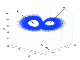
(b) Global attractor (the union of equilibria $S_{0,1,2}$ and local self-excited attractor).

(c) Global B-attractor (includes local self-excited attractor (blue), equilibria $S_{0,1,2}$, and their unstable manifold (green)).

Figure 3: Monostability. Numerical visualization of various types of attractors in system (3) with $b=1$, $\sigma=4$, $A=0.0052$, $r=687.5$.

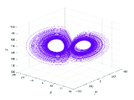
(a) Hidden attractor.

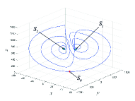
(b) B-attractor (includes equilibria $S_{0,1,2}$ and unstable manifold of $S_{0}$).

(c) Global attractor(the union of equilibria $S_{0,1,2}$ and local hidden attractor).

(d) Global B-attractor (the union of equilibria $S_{0,1,2}$, unstable manifold of $S_{0}$, and local hidden attractor).

Figure 4: Multistability. Numerical visualization of various types of attractors in system (3) with $b=1$, $\sigma=4$, $A=0.0052$, $r=700$.

Further we use the compact notations for the finite-time Lyapunov dimensions: $\dim_{\rm L}(t,u)=\dim_{\rm L}(\varphi^{t}_{\rm GD},u)$, $\dim_{\rm L}(t,K)=\dim_{\rm L}(\varphi^{t}_{\rm GD},K)$, and for the Lyapunov dimension: $\dim_{\rm L}K=\dim_{\rm L}(\{\varphi^{t}_{\rm GD}\}_{t\geq 0},K)$. For the chosen initial point $u_{0}=(x_{0},y_{0},z_{0})$ and time interval $[0,T]$, which are used to visualize the attractor $K$, there are the following substantial questions related to the computation of the finite-time Lyapunov dimension of $K$. The first question is whether there exists the limit $\lim_{t\to+\infty}\dim_{\rm L}(\varphi^{t},K)=\dim_{\rm L}K$ and, if not, whether for a given time interval $[0,T]$ the relation $\dim_{\rm L}(T,K)\leq\inf_{t\in[0,T)}\dim_{\rm L}(t,K)$ is true. In general, there is no rigorous justification of the choice of $t$ and it is known that unexpected jumps of $\dim_{\rm L}(t,K)$ can occur (see, e.g. Fig. 6). Thus it is reasonable to compute $\inf_{t\in[0,T)}\dim_{\rm L}(T,K)$ instead of $\dim_{\rm L}(T,K)$, but at the same time for any $T$ the value $\dim_{\rm L}(T,K)$ gives also a valid upper estimate for $\dim_{\rm H}K$. The second question is whether a given initial point $u_{0}$ belongs to the attractor $K$ or only to its basin of attraction (and thus the whole semi-orbit $\{\varphi^{t}_{\rm GD}(u_{0}),\ t\geq 0\}$ belongs only to the basin of attraction), and, if yes, whether $u_{0}$ is substantial for the Lyapunov dimension, i.e. whether the relation $\dim_{\rm L}(K)=\dim_{\rm L}(u_{0})$ is true or $\dim_{\rm L}(K)=\dim_{\rm L}(K\setminus u_{0})$. Since it is a challenging task to give justified answers to these questions, for numerical computation of the Lyapunov dimension we have to consider a dense grid of points $K_{\rm grid}$ on a numerical approximation (visualization) of $K$ and approximate the Lyapunov dimension of attractor $K$ by $\max_{u\in K_{\rm grid}}\dim_{\rm L}(t,u)$. Finally, in numerical experiments we can expect

$$\dim_{\rm H}K\leq\dim_{\rm L}K\approx$$

$$\qquad\qquad\approx\inf_{t\in[0,T]}\max_{u\in K_{\rm grid}}\dim_{\rm L}(t,u)=\max_{u\in K_{\rm grid}}\dim_{\rm L}(t_{\rm inf},u)\leq\max_{u\in K_{\rm grid}}\dim_{\rm L}(T,u)\approx\dim_{\rm L}(T,K).$$

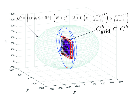
Figure 5: Localization of the hidden attractor by the absorbing set $\mathcal{B}^{h}$, cuboid $C^{h}=[-30,25]\times[-330,300]\times[395,956]$, and the corresponding grid of points $C^{h}_{\rm grid}$.

In Fig. 5 is shown the grid of points $C^{h}_{\rm grid}$ covering the hidden attractor: the grid points fill cuboid $C^{h}=[-30,25]\times[-330,300]\times[395,956]$ with the distance between points equals $5$; the grid of points $C^{se}_{\rm grid}$ covering self-excited attractor fill cuboid $C^{se}=[-25,25]\times[-305,290]\times[410,930]$). The time interval is $[0,\,60]$ and the integration method is MATLAB ode45. Remark that if for a certain time the computed trajectory is out of the cuboid, the corresponding value of finite-time local Lyapunov dimension does not taken into account in the computation of maximum of the finite-time local Lyapunov dimension (there are trajectories with initial data in cuboid, which are attracted to the zero equilibria, i.e. belong to its stable manifold, e.g. system (3) for $x=y=0$ is $\dot{z}=-bz$). The infimum on the time interval is computed at the points $\{t_{k}\}_{1}^{N}$ with time step $t_{\Delta}=t_{i+1}-t_{i}=0.1$. Note that if for a certain time $t=t_{k}$ the computed trajectory is out of the cuboid, the corresponding value of finite-time local Lyapunov dimension does not taken into account in the computation of maximum of the finite-time local Lyapunov dimension (there are trajectories with initial data in cuboid, which are attracted to the zero equilibria, i.e. belong to its stable manifold, e.g. system (3) for $x=y=0$ is $\dot{z}=-bz$). For the finite-time Lyapunov exponents (FTLE) computation we use MATLAB realization [21] of a method, based on SVD decompositions. For computation of the finite-time Lyapunov characteristic exponents (FTLCE) we use MATLAB realization [77] of a method, based on QR decompositions.

For both sets of parameters (see Fig. 3 and Fig. 4) we compute: 1) finite-time local Lyapunov dimensions $\dim_{\rm L}(60,\cdot)$ at the point $P_{1}=(10,60,800)$, which belong to both grids $C^{h,se}_{\rm grid}$, at the point $P_{2}=(-0.0074,-0.0997,0)$ on the unstable manifold of zero equilibria $S_{0}$; 2) maximums of the finite-time local Lyapunov dimensions at the points of grid $\max_{u\in C^{h,se}_{\rm grid}}\dim_{\rm L}(t,u)$ for the time points $t=t_{k}=0.1\,k$ $(k=1,..,600)$ and the infimum of the maximums; 3) the corresponding values, given by Kaplan-Yorke formula with respect to finite-time Lyapunov characteristic exponents. The results are given in Table 1 and 2.

Table 1: The set of parameters corresponding the self-excited attractor (see Fig. 3)

	$t=60$
$u=(10,60,800)$	$t=60$
$u=(-0.0074,-0.0997,0)$	$t=60$
$\max_{u\in C^{se}_{\rm grid}}$	$\displaystyle\inf_{t\in[0,\,60]}\max_{u\in C^{se}_{\rm grid}}$
$\dim_{\rm L}(t,\,u)$
(SVD)	$2.1345$	$2.1468$	$2.1721$	$2.1699$
${\scriptstyle{\rm d}_{\rm L}^{\rm KY}(\{{\rm LCE}_{i}(t,\,u)\}_{i=1}^{3})}$
(QR)	$2.1414$	$2.1262$	$2.1876$	$2.1854$

Table 2: The set of parameters corresponding the hidden attractor (see Fig. 4)

	$t=60$
$u=(10,60,800)$	$t=60$
$u=(-0.0074,-0.0997,0)$	$t=60$
$\max_{u\in C^{h}_{\rm grid}}$	$\displaystyle\inf_{t\in[0,\,60]}\max_{u\in C^{h}_{\rm grid}}$
$\dim_{\rm L}(t,\,u)$
(SVD)	$2.1271$	$1.2335$	$2.1638$	$2.1580$
${\scriptstyle{\rm d}_{\rm L}^{\rm KY}(\{{\rm LCE}_{i}(t,\,u)\}_{i=1}^{3})}$
(QR)	$2.1372$	$1.0139$	$2.1745$	$2.1735$

(a) Approximation via SVD based method.

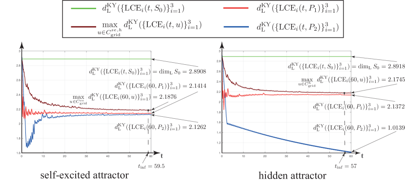
(b) Approximation via QR based method.

Figure 6: Dynamics of the finite-time local Lyapunov dimensions on the time interval $t\in[0,60]$: maximum on the grid of points (dark red), at the point $P_{1}=(10,\,60,\,800)\in C^{se,h}_{\rm grid}$ (light red), at $P_{2}=(-0.0074,\,-0.0997,\,0)$ from 1D unstable manifold of $S_{0}$ (blue); at the equilibrium $S_{0}$ (green).

The behavior of finite-time local Lyapunov dimensions for different points and their maximum on a grid of points is shown in Fig. 6. These values are in good correspondence with the exact Lyapunov dimension, obtained in Corollary 1. For the global attractor $K_{\text{global}}$ and global B-attractor $K_{\text{global B}}$ in Fig. 3(b,c) we have

$$\dim_{\rm L}K_{\text{global}}=\dim_{\rm L}K_{\text{global B}}=2.8908...$$

Since the global B-attractor $K_{\text{global B}}$ in Fig. 3(c) involves two-dimensional unstable manifolds of equilibria $S_{1,2}$, we have

$$2\leq\dim_{\rm H}K_{\text{global B}}\leq\dim_{\rm L}K_{\text{global B}}.$$

For the B-attractor $K_{\text{B}}$, the global attractor $K_{\text{global}}$, global B-attractor $K_{\text{global B}}$, in Fig. 4(b,c,d) we have

$$\dim_{\rm L}K_{\text{global}}=\dim_{\rm L}K_{\text{global B}}=\dim_{\rm L}K_{\text{B}}=2.8918...$$

Since the global B-attractor $K_{\text{global B}}$ in Fig. 4(d) involves one-dimensional unstable manifolds of equilibrium $S_{0}$, we have

$$1\leq\dim_{\rm H}K_{\text{global B}}\leq\dim_{\rm L}K_{\text{global B}}.$$

Remark that the absorbing sets $\mathcal{B}^{se}=\mathcal{B}(687.5,4,0.0052)$ and $\mathcal{B}^{h}=\mathcal{B}(700,4,0.0052)$ involve all the considered attractors in Fig. 3 and Fig. 4, respectively. Thus, for the corresponding grid of points by estimation (21) with $S=I$, we get an estimate for any attractor $K$ in Fig. 3 (here the distance between grid points is 20):

$$\dim_{\rm H}K\leq\dim_{\rm L}K\leq\sup_{u\in\mathcal{B}^{se}}d_{\rm L}^{\rm KY}\big{(}\{\lambda_{j}(u)\}_{i=1}^{n}\big{)}\approx\sup_{u\in\mathcal{B}^{se}_{\rm grid}}d_{\rm L}^{\rm KY}\big{(}\{\lambda_{j}(u)\}_{i=1}^{n}\big{)}=2.982747...\,,$$ (51)

and for any attractor $K$ in Fig. 4

$$\dim_{\rm H}K\leq\dim_{\rm L}K\leq\sup_{u\in\mathcal{B}^{h}}d_{\rm L}^{\rm KY}\big{(}\{\lambda_{j}(u)\}_{i=1}^{n}\big{)}\approx\sup_{u\in\mathcal{B}^{h}_{\rm grid}}d_{\rm L}^{\rm KY}\big{(}\{\lambda_{j}(u)\}_{i=1}^{n}\big{)}=2.983037...\,.$$ (52)

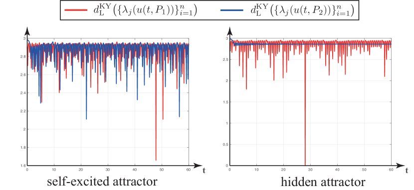
Figure 7: Dynamics of $d_{\rm L}^{\rm KY}\big{(}\{\lambda_{j}(u(t,P_{1}))\}_{i=1}^{n}\big{)}$ (red) and $d_{\rm L}^{\rm KY}\big{(}\{\lambda_{j}(u(t,P_{2}))\}_{i=1}^{n}\big{)}$ (blue) along the trajectories with initial data $P_{1}=(10,\,60,\,800)\in C^{se,h}_{\rm grid}$ and $P_{2}=(-0.0074,\,-0.0997,\,0)$.

The above numerical experiments lead to the following important conluding remarks. While the Lyapunov dimension, unlike the Hausdorff dimension, is not a dimension in the rigorous sense [57, 88] (e.g. the Lyapunov dimension of a saddle point or a periodic orbit can be noninteger and has different values including those close to $n$), it gives an upper estimate of the Hausdorff dimension. The sets with noninterger Hausdorff dimension are referred as the fractal sets [89]. Let the attractor $K$ or the corresponding absorbing set $\mathcal{B}\supset K$ is known (see, e.g. (6)). If one’s purpose is to demonstrate that $\dim_{\rm H}K\leq\dim_{\rm L}K<n$, then it can be achieved by Proposition 2 without integration of the considered dynamical system (see, e.g. (51) and (52)). In general, one can not expect to get the same values of the symmetrized Jacobian matrix eigenvalues at different points (see, e.g. Fig. 7), thus the maximum of $d_{\rm L}^{\rm KY}\big{(}\{\lambda_{j}(u)\}_{i=1}^{n}\big{)}$ on a grid of points has to be considered. If the purpose is to get a precise estimation of the Hausdorff dimension, then one can use (15) and have to compute the Lyapunov dimension. To be able to repeat a computation of Lyapunov dimension one need to know the considered compact invariant set $K$ and initial points of considered trajectories $\{u_{i}\}_{i=1}^{N}=K_{\rm grid}$ on the set, time interval $(0,T]=\bigcup_{i=0}^{M-1}(t_{i},t_{i+1}]$, and the method of Lyapunov exponents computation. Finite-time Lyapunov dimension is defined by singular values functions and for computing the corresponding Lyapunov exponents one has to use a numerical algorithms based on the SVD decomposition (not on the QR decomposition). While unexpected jumps in the values of the local Lyapunov exponents and Lyapunov dimension may occur, there is no rigorous justification of the choice of time $T$, and, thus, the $\inf_{t\in\{t_{i}\}_{i=0}^{M},t_{M}=T}$ of the finite-time Lyapunov dimensions often gives better estimates. In general, in numerical experiments one can not expect to get the same values of the finite-time local Lyapunov exponents and Lyapunov dimension for different points, thus the maximum of the finite-time local Lyapunov dimensions on the grid of point ($\max_{u\in K_{\rm grid}}$) has to be considered. Remark that in the work [66, p.190] Kaplan and Yorke called the limit values of the finite-time Lyapunov exponents $\{\lim\limits_{t\to+\infty}\operatorname{LE}_{i}(t,u)\}_{i=1}^{n}=\{\operatorname{LE}_{i}(u)\}_{i=1}^{n}$, if they exist and are the same for all $u\in K$ (and therefore [82] $\dim_{\rm L}K=d_{\rm L}^{\rm KY}(\{\operatorname{LE}_{i}(u_{0})\}_{i=1}^{n})$ for any $u_{0}\in K$), the absolute ones and wrote that such absolute values rarely exist.

5 Conclusion and further steps

In this paper the Lyapunov dimension of attractors in the Glukhovsky-Dolzhansky fluid convection model has been studied by analytical and numerical methods. In studying we follow a rigorous approach to the definition of the Lyapunov dimension and justification of its computation by the Kaplan-Yorke formula, without using statistical physics assumptions. The exact Lyapunov dimension formula for the global attractors is obtained and peculiarities of the Lyapunov dimension estimation for self-excited and hidden attractors are discussed. A tutorial on numerical estimation of the Lyapunov dimension on the example of the Glukhovsky-Dolzhansky model is presented.

References

- [1] P. Thompson, Numerical weather analysis and prediction, Macmillan New York, 1961.
- [2] A. Obukhov, On the problem of nonlinear interactions in fluid dynamics, Gerlands Beitraege zur Geophysik 82 (4) (1973) 282–290.
- [3] A. B. Glukhovsky, Nonlinear systems that are superpositions of gyrostats, Sov. Phys. Dokl. 27 (10) (1982) 823–825.
- [4] A. Gluhovsky, K. Grady, Effective low-order models for atmospheric dynamics and time series analysis, Chaos: An Interdisciplinary Journal of Nonlinear Science 26 (2) (2016) 023119.
- [5] E. N. Lorenz, Deterministic nonperiodic flow, J. Atmos. Sci. 20 (2) (1963) 130–141.
- [6] G. K. Vallis, El Niño: A chaotic dynamical system?, Science 232 (4747) (1986) 243–245.
- [7] A. B. Glukhovsky, F. V. Dolzhansky, Three component models of convection in a rotating fluid, Izv. Acad. Sci. USSR, Atmos. Oceanic Phys. 16 (1980) 311–318.
- [8] W. Tucker, The Lorenz attractor exists, Comptes Rendus de l’Academie des Sciences - Series I - Mathematics 328 (12) (1999) 1197 – 1202.
- [9] I. Stewart, Mathematics: The Lorenz attractor exists, Nature 406 (6799) (2000) 948–949.
- [10] P. J. Menck, J. Heitzig, N. Marwan, J. Kurths, How basin stability complements the linear-stability paradigm, Nature Physics 9 (2) (2013) 89–92.
- [11] A. Pisarchik, U. Feudel, Control of multistability, Physics Reports 540 (4) (2014) 167 218. doi:10.1016/j.physrep.2014.02.007.
- [12] D. Dudkowski, S. Jafari, T. Kapitaniak, N. Kuznetsov, G. Leonov, A. Prasad, Hidden attractors in dynamical systems, Physics Reports 637 (2016) 1–50. doi:10.1016/j.physrep.2016.05.002.
- [13] P. Grassberger, I. Procaccia, Measuring the strangeness of strange attractors, Physica D: Nonlinear Phenomena 9 (1-2) (1983) 189–208.
- [14] M. I. Rabinovich, Stochastic autooscillations and turbulence, Uspehi Physicheskih Nauk 125 (1) (1978) 123–168.
- [15] G. A. Leonov, V. A. Boichenko, Lyapunov’s direct method in the estimation of the Hausdorff dimension of attractors, Acta Applicandae Mathematicae 26 (1) (1992) 1–60.
- [16] A. S. Pikovski, M. I. Rabinovich, V. Y. Trakhtengerts, Onset of stochasticity in decay confinement of parametric instability, Sov. Phys. JETP 47 (1978) 715–719.
- [17] N. Kuznetsov, G. Leonov, T. Mokaev, S. Seledzhi, Hidden attractor in the Rabinovich system, Chua circuits and PLL, AIP Conference Proceedings 1738 (1), art. num. 210008.
- [18] G. Leonov, N. Kuznetsov, V. Vagaitsev, Localization of hidden Chua’s attractors, Physics Letters A 375 (23) (2011) 2230–2233. doi:10.1016/j.physleta.2011.04.037.
- [19] G. Leonov, N. Kuznetsov, V. Vagaitsev, Hidden attractor in smooth Chua systems, Physica D: Nonlinear Phenomena 241 (18) (2012) 1482–1486. doi:10.1016/j.physd.2012.05.016.
- [20] G. Leonov, N. Kuznetsov, Hidden attractors in dynamical systems. From hidden oscillations in Hilbert-Kolmogorov, Aizerman, and Kalman problems to hidden chaotic attractors in Chua circuits, International Journal of Bifurcation and Chaos 23 (1), art. no. 1330002. doi:10.1142/S0218127413300024.
- [21] G. Leonov, N. Kuznetsov, T. Mokaev, Homoclinic orbits, and self-excited and hidden attractors in a Lorenz-like system describing convective fluid motion, Eur. Phys. J. Special Topics 224 (8) (2015) 1421–1458. doi:10.1140/epjst/e2015-02470-3.
- [22] A. A. Andronov, E. A. Vitt, S. E. Khaikin, Theory of Oscillators, Pergamon Press, Oxford, 1966.
- [23] A. Jenkins, Self-oscillation, Physics Reports 525 (2) (2013) 167–222.
- [24] N. Kuznetsov, G. Leonov, V. Vagaitsev, Analytical-numerical method for attractor localization of generalized Chua’s system, IFAC Proceedings Volumes (IFAC-PapersOnline) 4 (1) (2010) 29–33. doi:10.3182/20100826-3-TR-4016.00009.
- [25] N. Kuznetsov, O. Kuznetsova, G. Leonov, V. Vagaitsev, Analytical-numerical localization of hidden attractor in electrical Chua’s circuit, Informatics in Control, Automation and Robotics, Lecture Notes in Electrical Engineering, Volume 174, Part 4 174 (4) (2013) 149–158. doi:10.1007/978-3-642-31353-0\_11.
- [26] N. Kuznetsov, Hidden attractors in fundamental problems and engineering models. A short survey., Lecture Notes in Electrical Engineering 371 (2016) 13–25, (Plenary lecture at AETA 2015: Recent Advances in Electrical Engineering and Related Sciences). doi:10.1007/978-3-319-27247-4\_2.
- [27] M. Shahzad, V.-T. Pham, M. Ahmad, S. Jafari, F. Hadaeghi, Synchronization and circuit design of a chaotic system with coexisting hidden attractors, European Physical Journal: Special Topics 224 (8) (2015) 1637–1652.
- [28] S. Brezetskyi, D. Dudkowski, T. Kapitaniak, Rare and hidden attractors in van der Pol-Duffing oscillators, European Physical Journal: Special Topics 224 (8) (2015) 1459–1467.
- [29] S. Jafari, J. Sprott, F. Nazarimehr, Recent new examples of hidden attractors, European Physical Journal: Special Topics 224 (8) (2015) 1469–1476.
- [30] Z. Zhusubaliyev, E. Mosekilde, A. Churilov, A. Medvedev, Multistability and hidden attractors in an impulsive Goodwin oscillator with time delay, European Physical Journal: Special Topics 224 (8) (2015) 1519–1539.
- [31] P. Saha, D. Saha, A. Ray, A. Chowdhury, Memristive non-linear system and hidden attractor, European Physical Journal: Special Topics 224 (8) (2015) 1563–1574.
- [32] V. Semenov, I. Korneev, P. Arinushkin, G. Strelkova, T. Vadivasova, V. Anishchenko, Numerical and experimental studies of attractors in memristor-based Chua’s oscillator with a line of equilibria. Noise-induced effects, European Physical Journal: Special Topics 224 (8) (2015) 1553–1561.
- [33] Y. Feng, Z. Wei, Delayed feedback control and bifurcation analysis of the generalized Sprott B system with hidden attractors, European Physical Journal: Special Topics 224 (8) (2015) 1619–1636.
- [34] C. Li, W. Hu, J. Sprott, X. Wang, Multistability in symmetric chaotic systems, European Physical Journal: Special Topics 224 (8) (2015) 1493–1506.
- [35] Y. Feng, J. Pu, Z. Wei, Switched generalized function projective synchronization of two hyperchaotic systems with hidden attractors, European Physical Journal: Special Topics 224 (8) (2015) 1593–1604.
- [36] J. Sprott, Strange attractors with various equilibrium types, European Physical Journal: Special Topics 224 (8) (2015) 1409–1419.
- [37] V. Pham, S. Vaidyanathan, C. Volos, S. Jafari, Hidden attractors in a chaotic system with an exponential nonlinear term, European Physical Journal: Special Topics 224 (8) (2015) 1507–1517.
- [38] S. Vaidyanathan, V.-T. Pham, C. Volos, A 5-D hyperchaotic Rikitake dynamo system with hidden attractors, European Physical Journal: Special Topics 224 (8) (2015) 1575–1592.
- [39] M.-F. Danca, Hidden transient chaotic attractors of Rabinovich–Fabrikant system, Nonlinear Dynamics 86 (2) (2016) 1263–1270.
- [40] I. Zelinka, Evolutionary identification of hidden chaotic attractors, Engineering Applications of Artificial Intelligence 50 (2016) 159–167.
- [41] G. Leonov, N. Kuznetsov, T. Mokaev, Hidden attractor and homoclinic orbit in Lorenz-like system describing convective fluid motion in rotating cavity, Communications in Nonlinear Science and Numerical Simulation 28 (2015) 166–174. doi:10.1016/j.cnsns.2015.04.007.
- [42] J. L. Kaplan, J. A. Yorke, Chaotic behavior of multidimensional difference equations, in: Functional Differential Equations and Approximations of Fixed Points, Springer, Berlin, 1979, pp. 204–227.
- [43] A. Douady, J. Oesterle, Dimension de Hausdorff des attracteurs, C.R. Acad. Sci. Paris, Ser. A. (in French) 290 (24) (1980) 1135–1138.
- [44] F. Ledrappier, Some relations between dimension and Lyapounov exponents, Communications in Mathematical Physics 81 (2) (1981) 229–238.
- [45] A. Eden, C. Foias, R. Temam, Local and global Lyapunov exponents, Journal of Dynamics and Differential Equations 3 (1) (1991) 133–177, [Preprint No. 8804, The Institute for Applied Mathematics and Scientific Computing, Indiana University, 1988]. doi:10.1007/BF01049491.
- [46] D. Russel, J. Hanson, E. Ott, Dimension of strange attractors, Physical Review Letters 45 (14) (1980) 1175–1178.
- [47] G. A. Leonov, On estimations of Hausdorff dimension of attractors, Vestnik St. Petersburg University: Mathematics 24 (3) (1991) 38–41, [Transl. from Russian: Vestnik Leningradskogo Universiteta. Mathematika, 24(3), 1991, pp. 41-44].
- [48] V. A. Boichenko, G. A. Leonov, V. Reitmann, Dimension Theory for Ordinary Differential Equations, Teubner, Stuttgart, 2005.
- [49] N. Kuznetsov, The Lyapunov dimension and its estimation via the Leonov method, Physics Letters A 380 (25–26) (2016) 2142–2149. doi:10.1016/j.physleta.2016.04.036.
- [50] G. Leonov, Lyapunov dimension formulas for Henon and Lorenz attractors, St.Petersburg Mathematical Journal 13 (3) (2002) 453–464.
- [51] G. Leonov, M. Poltinnikova, On the Lyapunov dimension of the attractor of Chirikov dissipative mapping, AMS Translations. Proceedings of St.Petersburg Mathematical Society. Vol. X 224 (2005) 15–28.
- [52] G. A. Leonov, Lyapunov functions in the attractors dimension theory, Journal of Applied Mathematics and Mechanics 76 (2) (2012) 129–141.
- [53] G. Leonov, A. Pogromsky, K. Starkov, Erratum to ”The dimension formula for the Lorenz attractor” [Phys. Lett. A 375 (8) (2011) 1179], Physics Letters A 376 (45) (2012) 3472 – 3474.
- [54] G. Leonov, N. Kuznetsov, N. Korzhemanova, D. Kusakin, Lyapunov dimension formula of attractors in the Tigan and Yang systems, arXiv:1510.01492v1 http://arxiv.org/pdf/1510.01492v1.pdf.
- [55] G. Leonov, T. Alexeeva, N. Kuznetsov, Analytic exact upper bound for the Lyapunov dimension of the Shimizu-Morioka system, Entropy 17 (7) (2015) 5101–5116. doi:10.3390/e17075101.
- [56] G. Leonov, N. Kuznetsov, N. Korzhemanova, D. Kusakin, Lyapunov dimension formula for the global attractor of the Lorenz system, Communications in Nonlinear Science and Numerical Simulation 41 (2016) 84–103. doi:10.1016/j.cnsns.2016.04.032.
- [57] W. Hurewicz, H. Wallman, Dimension Theory, Princeton University Press, Princeton, 1941.
- [58] E. Ott, W. Withers, J. Yorke, Is the dimension of chaotic attractors invariant under coordinate changes?, Journal of Statistical Physics 36 (5-6) (1984) 687–697.
- [59] N. Kuznetsov, T. Alexeeva, G. Leonov, Invariance of Lyapunov exponents and Lyapunov dimension for regular and irregular linearizations, Nonlinear Dynamics 85 (1) (2016) 195–201. doi:10.1007/s11071-016-2678-4.
- [60] G. Leonov, N. Kuznetsov, On differences and similarities in the analysis of Lorenz, Chen, and Lu systems, Applied Mathematics and Computation 256 (2015) 334–343. doi:10.1016/j.amc.2014.12.132.
- [61] G. Benettin, L. Galgani, A. Giorgilli, J.-M. Strelcyn, Lyapunov characteristic exponents for smooth dynamical systems and for hamiltonian systems. A method for computing all of them. Part 2: Numerical application, Meccanica 15 (1) (1980) 21–30.
- [62] A. Wolf, J. B. Swift, H. L. Swinney, J. A. Vastano, Determining Lyapunov exponents from a time series, Physica D: Nonlinear Phenomena 16 (D) (1985) 285–317.
- [63] A. M. Lyapunov, The General Problem of the Stability of Motion (in Russian), Kharkov, 1892, [English transl.: Academic Press, NY, 1966].
- [64] J. Tempkin, J. Yorke, Spurious Lyapunov exponents computed from data, SIAM Journal on Applied Dynamical Systems 6 (2) (2007) 457–474. doi:10.1137/040619211.
- [65] P. Augustova, Z. Beran, S. Celikovsky, ISCS 2014: Interdisciplinary Symposium on Complex Systems, Emergence, Complexity and Computation (Eds.: A. Sanayei et al.), Springer, 2015, Ch. On Some False Chaos Indicators When Analyzing Sampled Data, pp. 249–258.
- [66] P. Frederickson, J. Kaplan, E. Yorke, J. Yorke, The Liapunov dimension of strange attractors, Journal of Differential Equations 49 (2) (1983) 185–207.
- [67] J. Farmer, E. Ott, J. Yorke, The dimension of chaotic attractors, Physica D: Nonlinear Phenomena 7 (1-3) (1983) 153 – 180.
- [68] N. Bogoliubov, N. Krylov, La theorie generalie de la mesure dans son application a l’etude de systemes dynamiques de la mecanique non-lineaire, Ann. Math. II (in French) (Annals of Mathematics) 38 (1) (1937) 65–113.
- [69] M. Dellnitz, O. Junge, Set oriented numerical methods for dynamical systems, in: Handbook of Dynamical Systems, Vol. 2, Elsevier Science, 2002, pp. 221–264.
- [70] V. Oseledets, A multiplicative ergodic theorem. Characteristic Ljapunov, exponents of dynamical systems, Trudy Moskovskogo Matematicheskogo Obshchestva (in Russian) 19 (1968) 179–210.
- [71] L. Barreira, J. Schmeling, Sets of “Non-typical” points have full topological entropy and full Hausdorff dimension, Israel Journal of Mathematics 116 (1) (2000) 29–70.
- [72] P. Cvitanović, R. Artuso, R. Mainieri, G. Tanner, G. Vattay, Chaos: Classical and Quantum, Niels Bohr Institute, Copenhagen, 2012, http://ChaosBook.org.
- [73] W. Ott, J. Yorke, When Lyapunov exponents fail to exist, Phys. Rev. E 78 (2008) 056203.
- [74] L.-S. Young, Mathematical theory of Lyapunov exponents, Journal of Physics A: Mathematical and Theoretical 46 (25) (2013) 254001.
- [75] G. Leonov, N. Kuznetsov, Time-varying linearization and the Perron effects, International Journal of Bifurcation and Chaos 17 (4) (2007) 1079–1107. doi:10.1142/S0218127407017732.
- [76] J. Schmeling, A dimension formula for endomorphisms – the Belykh family, Ergodic Theory and Dynamical Systems 18 (1998) 1283–1309.
- [77] N. Kuznetsov, T. Mokaev, P. Vasilyev, Numerical justification of Leonov conjecture on Lyapunov dimension of Rossler attractor, Commun Nonlinear Sci Numer Simulat 19 (2014) 1027–1034.
- [78] R. Smith, Some application of Hausdorff dimension inequalities for ordinary differential equation, Proc. Royal Society Edinburg 104A (1986) 235–259.
- [79] K. Gelfert, Maximum local Lyapunov dimension bounds the box dimension. Direct proof for invariant sets on Riemannian manifolds, Z. Anal. Anwend. 22 (2003) 553–568.
- [80] A. Eden, Local estimates for the Hausdorff dimension of an attractor, Journal of Mathematical Analysis and Applications 150 (1) (1990) 100–119.
- [81] P. Constantin, C. Foias, R. Temam, Attractors representing turbulent flows, Memoirs of the American Mathematical Society 53 (314).
- [82] N. Kuznetsov, G. Leonov, A short survey on Lyapunov dimension for finite dimensional dynamical systems in Euclidean space, arXivHttp://arxiv.org/pdf/1510.03835v2.pdf.
- [83] C. Doering, J. Gibbon, D. Holm, B. Nicolaenko, Exact Lyapunov dimension of the universal attractor for the complex Ginzburg-Landau equation, Phys. Rev. Lett. 59 (1987) 2911–2914.
- [84] G. A. Leonov, T. N. Mokaev, Lyapunov dimension formula for the attractor of the Glukhovsky-Dolzhansky system, Doklady Mathematics 93 (1) (2016) 42–45.
- [85] A. Eden, An abstract theory of L-exponents with applications to dimension analysis (PhD thesis), Indiana University, 1989.
- [86] G. Leonov, S. Lyashko, Eden’s hypothesis for a Lorenz system, Vestnik St. Petersburg University: Mathematics 26 (3) (1993) 15–18, [Transl. from Russian: Vestnik Sankt-Peterburgskogo Universiteta. Ser 1. Matematika, 26(3), 14-16].
- [87] C. R. Doering, J. Gibbon, On the shape and dimension of the Lorenz attractor, Dynamics and Stability of Systems 10 (3) (1995) 255–268.
- [88] K. Kuratowski, Topology, Academic press, New York, 1966.
- [89] J.-P. Eckmann, D. Ruelle, Ergodic theory of chaos and strange attractors, Reviews of Modern Physics 57 (3) (1985) 617–656.