Radiative lifetime and energy of the low-energy isomeric level in ²²⁹Th

Abstract

We estimate the range of the radiative lifetime and energy of the anomalous, low-energy $3/2^{+}(7.8\pm 0.5$ eV) state in the ²²⁹Th nucleus. Our phenomenological calculations are based on the available experimental data for the intensities of $M1$ and $E2$ transitions between excited levels of the ²²⁹Th nucleus in the $K^{\pi}[Nn_{Z}\Lambda]=5/2^{+}[633]$ and $3/2^{+}[631]$ rotational bands. We also discuss the influence of certain branching coefficients, which affect the currently accepted measured energy of the isomeric state. From this work, we establish a favored region where the transition lifetime and energy should lie at roughly the 90% confidence level. We also suggest new nuclear physics measurements, which would significantly reduce the ambiguity in the present data.

I Introduction

The low-energy isomeric state in the ²²⁹Th nucleus is currently a subject of intense experimental and theoretical research (see a short review of the literature in Browne and Tuli (2008); Jeet et al. (2015) and references below). This state is expected to provide access to a number of interesting physical effects, including the decay of the nuclear isomeric level via the electronic bridge mechanism in certain chemical environments Strizhov and Tkalya (1991); Porsev and Flambaum (2010a, b), cooperative spontaneous emission Dicke (1954) in a system of excited nuclei, the Mößbauer effect in the optical range Tkalya (2011), sensitive tests of the variation of the fine structure constant and the strong interaction parameter Flambaum (2006); He and Ren (2007); Hayes and Friar (2007); Litvinova et al. (2009), a check of the exponentiality of the decay law of an isolated metastable state at long times Dykhne and Tkalya (1998a), and accelerated $\alpha$-decay of the ²²⁹Th nuclei via the low energy isomeric state Dykhne et al. (1996). In addition, two applications that may have a significant technological impact were proposed: a new metrological standard for time Tkalya et al. (1996) or the “nuclear clock” Peik and Tamm (2000); Rellergert et al. (2010a); Campbell et al. (2012); Peik and Okhapkin (2015), and a nuclear laser (or gamma ray laser) in the optical range Tkalya (2011).

The ground state of the ²²⁹Th nucleus, $J^{\pi}E=5/2^{+}(0.0)$, is the ground level of the rotational band $K^{\pi}[Nn_{Z}\Lambda]=5/2^{+}[633]$. Currently, there is little doubt in the existence of the low-energy isomeric level $J^{\pi}E=3/2^{+}(E_{is})$, which is the lowest level of the rotational band $K^{\pi}[Nn_{Z}\Lambda]=3/2^{+}[631]$. The existence of the other levels of this band is reliably experimentally validated Browne and Tuli (2008). In addition, an independent corroboration of the existence of a low-lying state has been achieved experimentally in the reaction ²³⁰Th$(d,t)^{229}$Th Burke et al. (2008). This experiment provides strong evidence that the $K^{\pi}[Nn_{Z}\Lambda]=3/2^{+}[631]$ band head is located very close to the ground state, and, in fact, all available experimental data from these indirect measurements of the $J^{\pi}K[Nn_{Z}\Lambda]=3/2^{+}3/2[631]$ isomeric state energy indicate that $E_{is}<10$ eV Helmer and Reich (1994); Guimaraes-Filho and Helene (2005); Beck et al. (2007); Bec (a).

Unfortunately, the energy resolution of such experiments does not provide the accuracy required for direct optical spectroscopy of the nuclear isomeric $M$1 transition $5/2^{+}5/2[633](0.0)\leftrightarrow 3/2^{+}3/2[631](E_{is})$, which is clearly a prerequisite for the aforementioned studies. Therefore, new approaches to determine the isomeric energy are required. While there are some ongoing attempts to better measure the isomeric transition energy (see for example Zhao et al. (2012)), directly driving the nuclear transition inside an insulator with a large band gap (i.e. a crystal), first proposed in the works Tkalya (2000); Tkalya et al. (2000), or in sample of trapped ions Kälber et al. (1989); Campbell et al. (2009); Herrera-Sancho et al. (2012) appear to be the most promising routes forward in the short term.

In the crystal approach, a band gap greater than $E_{is}$ results in the absence of the conversion decay channel of the low energy isomeric state. Thus, the uncertainty in the decay probability, which is associated with electronic conversion, disappears. In Ref. Rellergert et al. (2010a, b); Hehlen et al. (2013) the requirements and characteristics of the requisite crystals were made rigorous, showing that ²²⁹Th:LiCaAlF₆ and ²²⁹Th:LiSrAlF₆ were likely good choices; other efforts focus on CaF₂ Dessovic et al. (2014); Stellmer et al. (2015), or ThF₄ and Na₂ThF₆ Ellis et al. (2014). Several experiments using this solid-state approach have been carried out in recent years Zhao et al. (2012); Yamaguchi et al. (2015); Jeet et al. (2015), though as described in Sec. III, care must be taken to interpret the results of these experiments.

Experiments using trapped Th⁺ Herrera-Sancho et al. (2012); Okhapkin et al. (2015) or Th³⁺ Campbell et al. (2009, 2011); Radnaev et al. (2012); Beloy (2014) ions aim at exploiting the electronic bridge process Strizhov and Tkalya (1991); Porsev and Flambaum (2010a, b), which can dominate the direct radiative decay of the isomeric transition. Using the electronic bridge process and exciting the isomeric transition in a multi-photon nucleon-electron simultaneous transition has the potential advantage of obviating the use of a vacuum ultraviolet laser system, at the expense of a modest increase in system complexity. Experiments have advanced rapidly in recent years and it is expected that with recent high-resolution electronic spectra Campbell et al. (2011); Radnaev et al. (2012); Herrera-Sancho et al. (2013); Okhapkin et al. (2015), electronic bridge excitation rates can be better calculated in the near future.

In any experiment searching for the nuclear energy level, two key parameters in the preparation of the experiment are the isomeric state lifetime and energy. Therefore, the aim of this manuscript is to provide a critical assessment and estimation of these parameters to aid these experiments. In Section II of this paper, we analyze the experimental data on the nuclear matrix elements of transitions between states belonging to rotational bands $K^{\pi}[Nn_{Z}\Lambda]=5/2^{+}[633]$ and $3/2^{+}[631]$ both in ²²⁹Th only and in comparable nuclei. In Section III, we estimate the radiative lifetime of the isomeric state using available experimental data for the transition rates of the interband $M$1 and $E$2 gamma transitions between excited levels of the ²²⁹Th nucleus. In Section IV we consider the importance of the conversion decay channel, showing that these processes will dominate the isomer radiative decay in cases where they are possible and, therefore, must be avoided. In Section V, we analyze the possible range of branching coefficients. We show how this range affects the determination of the isomeric energy in the experiments of Refs. Beck et al. (2007); Bec (b), which provide the currently accepted isomeric transition energy range. In Section VI, we briefly discuss the results of this work and present a “favored region”, which we recommend the community adopt in order to direct future searches. We conclude in Section VII with a summary of these results and point out new nuclear physics measurements that should be performed to considerably reduce the uncertainty in the present data.

In the present work, we use (if not noted otherwise) the following system of units: $\hbar=c=1$.

II Matrix element of the isomeric transition

Together with the energy of the isomeric level, the magnitude of the nuclear transition matrix element determines the half life $T_{1/2}$ or the radiative lifetime $\tau$ ($\tau=T_{1/2}/\ln(2)$) of the isomeric state. Currently, there are two possibilities for phenomenological estimation of the reduced probability for the isomeric transition, $B(M1;3/2^{+}3/2[631]\rightarrow 5/2^{+}5/2[633])$. The first possibility is to use parameters of the similar 311.9 keV transition in the spectrum of the ²³³U nucleus. The second is to take advantage of the available experimental data for the $M$1 transitions between the rotational bands $K^{\pi}[Nn_{Z}\Lambda]=5/2^{+}[633]$ and $3/2^{+}[631]$ in the excitation spectrum of the ²²⁹Th nucleus.

The first method can be motivated, because transitions $3/2^{+}3/2[631]\rightarrow 5/2^{+}5/2[633]$ at 311.9 keV in the ²³³U nucleus and 7.8 eV in the ²²⁹Th nucleus look identical in terms of the rotational model and, in that context, should have the same reduced transition probabilities. (In this and the following section, we will use the updated value of Ref. Bec (b) for the ²²⁹Th isomeric energy, $E_{is}=7.8\pm 0.5$ eV; see Section V for further discussion of the isomeric state energy.) The reduced probability of the transition in the ²³³U nucleus is known to be $B_{W.u.}(M1;3/2^{+}3/2[631](311.9$ keV$)\rightarrow 5/2^{+}5/2[633](0.0))=(0.33\pm 0.05)\times 10^{-2}$ Singh and Tuli (2005). Here, $B_{W.u.}$ denotes a reduced probability in Weisskopf units Bla (see Appendix A for details):

$$B_{W.u.}(M1;J_{i}\rightarrow{}J_{f})=\frac{B(M1;J_{i}\rightarrow{}J_{f})}{B(W;M1)}\,,$$ (1)

where $B(W;M1)=(45/8\pi)\mu_{N}^{2}$ is the reduced probability of the nuclear $M$1 transition in the Weisskopf model and $\mu_{N}$ is the nuclear magneton.

Nonetheless, the ²³³U and ²²⁹Th nuclei are different and those differences could be crucial, which becomes evident when comparing to other nuclei with similar level structure. For example, a $3/2^{+}3/2[631]\rightarrow 5/2^{+}5/2[633]$ transition with an energy of 221.4 keV also exists in the ²³¹Th nucleus Browne and Tuli (2013). The half life of the $3/2^{+}3/2[631](221.4$ keV) state in ²³¹Th is less than 74 ps and only one gamma transition, namely, the transition to the ground state has been observed experimentally from this level, with an internal conversion coefficient of 1.96 Browne and Tuli (2013). This is not surprising since according to the level scheme Browne and Tuli (2013), the quantum numbers of states lying between the $3/2^{+}3/2[631](221.4$ keV) level and the ground state are such that the intensity of other possible transitions must be orders of magnitude smaller than the $3/2^{+}3/2[631](221.4$ keV$)\rightarrow 5/2^{+}5/2[633](0.0)$ transition. Therefore, the transition directly to the ground state should give the dominant contribution to the decay of the level in the ²³¹Th nucleus, and the other decay channels cannot significantly change the lifetime of the level. Using the data from Ref. Browne and Tuli (2013) the reduced probability of this transition in the ²³¹Th nucleus is estimated as $B_{W.u.}(M1;3/2^{+}3/2[631](221.4$ keV$)\rightarrow 5/2^{+}5/2[633](0.0))\geq 0.93\times 10^{-2}$. This value is at least three times larger than would have been expected estimating it from the similar transition in ²³³U. Accordingly, interpolation from the ²³³U nucleus to the ²²⁹Th nucleus could lead to similar results. In addition, it is not obvious that measurements of the nuclear lifetimes, $\gamma$-ray intensities, the probabilities of electronic conversion, and other characteristics of this transition in the ²³³U nucleus are more accurate than for the ²²⁹Th nucleus, where measurement errors, as we shall see below, are significant.

For these reasons, we prefer to use the second approach to determine an estimate of $B(M1;3/2^{+}3/2[631](7.8$ eV)$\rightarrow 5/2^{+}5/2[633](0.0))$, which relies on available experimental data for the reduced probability of the $M$1 transitions between the rotational bands $K^{\pi}[Nn_{Z}\Lambda]=5/2^{+}[633]$ and $3/2^{+}[631]$ in the ²²⁹Th nucleus and the Alaga rules. Such a calculation assumes that the adiabatic condition is fulfilled (see Dykhne and Tkalya (1998b) for a detailed analysis of the use of the adiabatic condition). Here, we do not consider the effects of nonadiabaticity because of the relatively large uncertainties and disagreements of the experimental data (see Fig. 1). Further, the well-expressed rotational structure of the bands in the ²²⁹Th nucleus and a number of other factors Dykhne and Tkalya (1998b) allow us to neglect the Coriolis interaction for a preliminary estimation of the reduced probability of the isomeric transition from the experimental data for the $9/2^{+}5/2[633](97.14$ keV$)\rightarrow 7/2^{+}3/2[631](71.83$ keV) transition in the ²²⁹Th nucleus. In this limit, we can, however, provide an estimate of the effect of the Coriolis interaction, which is quite small, on the matrix element Dykhne and Tkalya (1998b).

Experimental data for $B(M1;9/2^{+}5/2[633](97.14$ keV$)\rightarrow 7/2^{+}3/2[631](71.83$ keV)) are, to our knowledge, available from four separate experiments C. E. Bemis et al. (1988); Gulda et al. (2002); Barci et al. (2003); Ruchowska et al. (2006). As can be seen in Fig. 1, the reported values for the $M$1 transition show considerable spread. For comparison, in the case of the $E$2 transition, there is consensus between three of the measurements.

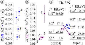
Figure 1: (color online). The experimental values for the reduced probability of the nuclear (a) $9/2^{+}(97.14$ keV)$\rightarrow 7/2^{+}(71.83$ keV), and (b) $9/2^{+}(97.14$ keV)$\rightarrow 5/2^{+}(29.19$ keV) transitions The relevant level scheme of the ²²⁹Th nucleus is shown in part (c). Data for the transitions were taken from: 1 – C. E. Bemis et al. (1988), 2 – Gulda et al. (2002), 3 – Barci et al. (2003), and 4 – Ruchowska et al. (2006).

Using the Alaga rules, it is straightforward to obtain the reduced probability of the isomeric nuclear transition in terms of the measured $M$1 reduced probability:

$$B(M1;3/2^{+}(7.8\leavevmode\nobreak\ {\text{eV}})\rightarrow 5/2^{+}(0.0))\\ =\frac{15}{7}B(M1;9/2^{+}(97.14\leavevmode\nobreak\ {\text{keV}})\rightarrow 7/2^{+}(71.83\leavevmode\nobreak\ {\text{keV}}))\,.$$

The results of this calculation are shown in Table 1 for each measured value of $B(M1;9/2^{+}5/2[633](97.14$ keV$)\rightarrow 7/2^{+}3/2[631](71.83$ keV)) from Fig. 1(a).

Table 1: Calculated reduced probabilities $B_{W.u.}(M1;3/2^{+}(7.8\leavevmode\nobreak\ {\text{eV}})\rightarrow 5/2^{+}(0.0))$ in ²²⁹Th based on $B(M1;9/2^{+}5/2[633](97.14$ keV$)\rightarrow 7/2^{+}3/2[631](71.83$ keV) from given references.

$B_{W.u.}$ ($10^{-2}$)	based on
$3.83\pm 0.72$	Ref. C. E. Bemis et al. (1988)
$1.42\pm 0.30$	Ref. Gulda et al. (2002)
$2.41\pm 0.29$	Ref. Barci et al. (2003)
$4.55\pm 0.48$	Ref. Ruchowska et al. (2006)

Interestingly, the data of Barci et al. (2003) affords another means to obtain $B_{W.u.}(M1;3/2^{+}(7.8\leavevmode\nobreak\ {\text{eV}})\rightarrow 5/2^{+}(0.0))$. In that work, the relative intensities of the transitions from the level $9/2^{+}3/2[631](125.44\leavevmode\nobreak\ {\text{keV}})$ were also measured to states $9/2^{+}(97.14\leavevmode\nobreak\ {\text{keV}})$ and $7/2^{+}(42.44\leavevmode\nobreak\ {\text{keV}})$ of the $5/2^{+}[633]$ rotational band. This allows us to calculate the reduced probabilities $B(M1;9/2^{+}3/2[631](125.44\leavevmode\nobreak\ {\text{keV}})\rightarrow 9/2^{+}5/2[633](97.14\leavevmode\nobreak\ {\text{keV}}))=(0.56\pm 0.25)\times 10^{-2}$ $\mu_{N}^{2}$ and $B(M1;9/2^{+}3/2[631](125.44\leavevmode\nobreak\ {\text{keV}})\rightarrow 7/2^{+}5/2[633](42.44\leavevmode\nobreak\ {\text{keV}}))=(0.9\pm 0.4)\times 10^{-3}$ $\mu_{N}^{2}$ in the frame of the rotational model. Using the Alaga rules, we can then calculate the reduced probability of the $M$1(7.8 eV) isomeric transition. Both of the reduced probabilities give practically the same value $B_{W.u.}(M1;3/2^{+}(7.8\leavevmode\nobreak\ {\text{eV}})\rightarrow 5/2^{+}(0.0))=(0.74\pm 0.33)\times 10^{-2}$. This result is shown in Table 2 along with the reduced probabilities of similar transitions in ²³³U at 311.9 keV and ²³¹Th at 221.4 keV.

Table 2: Reduced probabilities $B_{W.u.}(M1;3/2^{+}3/2[631]\rightarrow 5/2^{+}5/2[633])$ for other nuclei or, for the case of ²²⁹Th, calculated from reduced probabilities of other transitions (see text).

$B_{W.u.}$ ($10^{-2}$)	nucleus	from/based on
$0.33\pm 0.05$	233U	Ref. Singh and Tuli (2005)
$>0.93$	231Th	Ref. Browne and Tuli (2013)
$0.74\pm 0.33$	229Th	Ref. Barci et al. (2003)

Thus, these estimates lead to a significant, more than an order of magnitude, range in the values for the reduced probability of the isomeric transition of the ²²⁹Th nucleus. However, if, for the aforementioned reasons, we restrict the estimate to those values calculated from the $9/2^{+}5/2[633](97.14\leavevmode\nobreak\ {\text{keV}})\rightarrow 7/2^{+}3/2[631](71.83\leavevmode\nobreak\ {\text{keV}})$ transitions the spread in mean values is within a factor of 3.

III Radiative lifetime of the isomeric level

Currently, the generally accepted value for the energy of the isomeric state $3/2^{+}3/2[631]$ is $7.8\pm 0.5$ eV Beck et al. (2007); Bec (b). Since the energy of the isomeric level exceeds, for example, the ionization potential of the isolated thorium atom, 6.08 eV, the radiative lifetime of the ²²⁹Th isomeric state is highly dependent on the chemical environment and electronic conversion is the dominant decay channel Strizhov and Tkalya (1991). It is very difficult to directly observe the transition in such environments, as both the excitation radiation is absorbed by the electrons and the energy of any conversion electron is very small (only a few electron volts), making it difficult to detect. Similarly, it is difficult to predict the lifetime of the isomeric state for thorium ions in the Th^m+, $m<4$ charge state. Here, for example, the process of decay via the electronic bridge Strizhov and Tkalya (1991); Porsev and Flambaum (2010a, b) can dominate, which cannot be calculated without precise knowledge of the nuclear transition energy and the wave functions of the valence electrons.

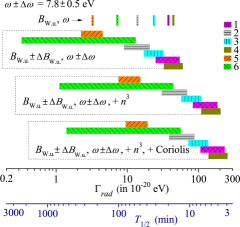
Figure 2: (color online). The range of possible radiative linewidths $\Gamma_{rad}$ (upper scale) and half-lifes $T_{1/2}$ (lower scale) of the isomeric state $3/2^{+}3/2[631](7.8\pm 0.5\leavevmode\nobreak\ {\text{eV}})$ in the ²²⁹Th nucleus. Calculations are based on values for $B_{W.u.}(M1;3/2^{+}3/2[631]\rightarrow 5/2^{+}5/2[633])$ from Tab. 1 (calculated from: 1 – C. E. Bemis et al. (1988), 2 – Gulda et al. (2002), 3 – Barci et al. (2003), 4 – Ruchowska et al. (2006)) and, for completeness, Tab. 2 (5 – Singh and Tuli (2005); 6 – Barci et al. (2003)). The refractive index $n\approx 1.5$ increases the probability of the $M$1 transition by a factor $n^{3}$ (third row). The Coriolis interaction can lead to a slight increase of the linewidth by a factor of 1.2–1.3 Dykhne and Tkalya (1998a) (fourth row).

In the following, we only estimate the radiative half-life of the thorium isomeric state in the absence of any chemical effects based on the reduced probabilities discussed in Sec. II. As discussed previously, we prefer the four reduced probabilities calculated from the four measurements for the $M$1 $9/2^{+}5/2[633](97.14\leavevmode\nobreak\ {\text{keV}})\rightarrow 7/2^{+}3/2[631](72.83\leavevmode\nobreak\ {\text{keV}})$ transition in ²²⁹Th (see Tab. 1), which appears most defensible, as this technique has shown to be accurate to within experimental error in cases where data exists Dykhne and Tkalya (1998b). Radiative half-lifes based on the reduced probabilities from other transitions in ²²⁹Th or the similar transition in ²³³U are only given for completeness (see Tab. 2). These results are directly applicable to trapped Th^m+ ions with $m\geq 4$ and, with a minor modification, to Th in a large-bandgap crystal. The modification in the latter case is due to the polarization of the dielectric medium and leads to a reduction of the half-life by a factor of $1/n^{3}$ Rikken and Kessener (1995); Tkalya (2000), where $n$ denotes the refractive index. The calculated half-lifes can further be used in the trapped ion approach with $m<4$ to calculate e.g. the electron bridge process once the electronic spectra of the ions are known.

The results are shown in Fig. 2, first row, for $\omega=7.8\,\mathrm{eV}$. The range of half-lifes including one standard deviation in both the reduced probabilities and the currently accepted transition energy is given in the second row. The calculations for the case of a large-bandgap crystal with a typical refractive index $n\approx 1.5$ is shown in the third row. Lastly, the additional inclusion of the Coriolis interaction leads to only a small correction (fourth row).

Using these results, we construct a favored region for the radiative half-life as a function of transition energy based only on the values for the reduced probabilities from Tab. 1 (see also Fig. 5 in Sec. VI). The center of this favored region is defined by the weighted average of the reduced probabilities. The bounds of the favored region are constructed as 1.96 standard deviations around the center of the favored region, which corresponds to roughly a 95% confidence level, however, considering that the individual reduced transition probabilities are not consistent within their errors, we increase the standard deviation by the Birge ratio of 3.4 Bodnar and Elster (2014):

$$0.46\times 10^{6}\leavevmode\nobreak\ {\text{s\leavevmode\nobreak\ eV}}^{3}/\omega^{3}\leq T_{1/2}\leq 1.5\times 10^{6}\leavevmode\nobreak\ {\text{s\leavevmode\nobreak\ eV}}^{3}/\omega^{3}.$$

Here, we did not include a crystal environment, as the inclusion of the refractive index $n$ is straightforward. However, the small correction due to Coriolis interaction is included leading to an increase of the linewidth of the transition by a factor of 1.2–1.3 Dykhne and Tkalya (1998b). (These bounds are similar to those of Ref. Jeet et al. (2015), but we consider them more accurate as they include e.g. the Birge ratio.)

Alternatively, a more conservative region can be constructed which is bound by the extreme values of the individual radiative lifetimes deduced from Tab. 1 $\pm 1.96$ standard deviations (see Fig. 5). Its functional form is given as (again including correction due to Coriolis interaction, but without crystal environment):

$$0.31\times 10^{6}\leavevmode\nobreak\ {\text{s\leavevmode\nobreak\ eV}}^{3}/\omega^{3}\leq T_{1/2}\leq 2.1\times 10^{6}\leavevmode\nobreak\ {\text{s\leavevmode\nobreak\ eV}}^{3}/\omega^{3}.$$

IV Importance of the electronic conversion decay channel

As mentioned in Sec. III, the chemical environment can significantly affect the half-life of the isomeric state Strizhov and Tkalya (1991). It most likely explains why, given the currently accepted value for the isomeric transition energy, that many previous experiments performed in powders, solids and solutions produced null results Browne et al. (2001); Kikunaga et al. (2009); Mitsugashira et al. (2003); Zimmermann (2010); Swanberg Jr. (2012); similarly, non-VUV sensitive measurements could have been affected by internal conversion Utter et al. (1999); Shaw et al. (1999). The internal conversion process could also have strong implications for the experiments reported in Refs. Zhao et al. (2012) and Yamaguchi et al. (2015). Though crystalline material is used as host in these experiments, the charge state of the thorium atom is not known, since the thorium atoms are either implanted into Zhao et al. (2012) or chemically adsorbed onto the surface of Yamaguchi et al. (2015) the crystal. Therefore, it is likely that some, if not all, of the thorium atoms are in a local chemical environment that experiences electronic conversion. As we will see in the following, it is unlikely the isomeric transition can be detected in such a system, if internal conversion is present. Thus, as aptly pointed out in Ref. Yamaguchi et al. (2015), any conclusions drawn from experiments of this type should be considered preliminary until the thorium chemical environment is known.

If the energy of the isomeric level $3/2^{+}3/2[631]$ in the ²²⁹Th exceeds the binding energy of electrons in the local chemical environment, the main channel of decay is electronic conversion Strizhov and Tkalya (1991). Therefore, the lifetime of the isomeric state can be significantly reduced compared to the radiative lifetime only. In the following, we consider electronic conversion of the isomeric state in the neutral Th atom as an example to give a rough estimate of the lifetime for the ²²⁹Th isomeric state in such a chemical environment.

Electronic $M$1 and $E$2 conversion from the valence 6$d$ and 7$s$ shells of the thorium atom is possible for the nuclear isomeric transition. The ratio of radiation widths of the $E$2 and $M$1 transitions with energy of 7.8 eV in the ²²⁹Th nucleus is $\Gamma_{rad}(W;E2)/\Gamma_{rad}(W;M1)\simeq 10^{-13}$ in the Weisskopf model, i.e. when the nuclear reduced probabilities are $B_{W.u.}(M1)=1$ and $B_{W.u.}(E2)=1$. Therefore, we can neglect the $E$2 contribution to the radiation width of the level for true values in the ranges $B_{W.u.}(M1;3/2^{+}(7.8\leavevmode\nobreak\ {\text{eV}})\rightarrow 5/2^{+}(0.0))\simeq 10^{-1}$–$10^{-3}$ and $B_{W.u.}(E2;3/2^{+}(7.8\leavevmode\nobreak\ {\text{eV}})\rightarrow 5/2^{+}(0.0))\simeq 1$–10, respectively. As for the conversion decay channel, our calculations for the thorium atom give the relation $\Gamma_{conv}(W;E2)/\Gamma_{conv}(W;M1)\simeq 10^{-6}$ in the Weisskopf model. Accordingly, for the true range of values for the reduced probabilities we find $\Gamma_{conv}(E2)/\Gamma_{conv}(M1)\leq 10^{-3}$ for a transition with energy of 7.8 eV in the ²²⁹Th nucleus. Thus, we neglect the contribution of electronic $E$2 conversion to the isomeric state conversion lifetime.

The calculation of the probability $\Gamma_{conv}$ was performed using code developed in Sol on the basis of known code in Band and Fomichev (1979), and then advanced in Strizhov and Tkalya (1991). The calculated electronic $M$1 conversion probability for the energy range 7.3 eV – 8.3 eV, using the reduced probabilities from Tables 1 and 2, are presented in Figure 3. Taking into account the uncertainties on the magnitude of the nuclear matrix element of the transition, the characteristic lifetime of the isomer in an atom is $\sim 10\,\mathrm{\mu s}$. As a result, electronic conversion completely quenches the isomeric state non-radiatively. Thus, experiments looking for the emitted photons as a signal of the isomeric transition must ensure that the local chemical environment of the thorium atom does not support electronic conversion.

Figure 3: (color online). The ranges of possible conversion widths (the upper scale) and lifetimes (the lower scale) of the isomeric nuclear state in a neutral isolated Th atom. The designations are identical with designations in Fig. 2.

However, this is only one side of the issue. The $M$1 isomeric transition like the other $M$1 transitions between states of the bands $K^{\pi}[Nn_{Z}\Lambda]=5/2^{+}[633]$ and $3/2^{+}[631]$, is first-order forbidden by the asymptotic quantum numbers of the Nilsson model Nilsson (1955). Indeed, we are considering $M$1 transitions where $\Delta{}K=1$, $\Delta{}N=0$, $\Delta{}n_{Z}=0$, and $\Delta\Lambda=2$, while the selection rules for the $M$1 transition allow the following change for the asymptotic quantum numbers for the case $\Delta{}K=1$: $\Delta{}N_{a}=0,\pm 2$, $\Delta{}n_{Z_{a}}=0,\pm 1$, and $\Delta\Lambda_{a}=0,\pm 1$ Nilsson (1955) (the index $a$ means “allowed”). Thus, the interband $M$1 transitions $K^{\pi}[Nn_{Z}\Lambda]=5/2^{+}[633]\leftrightarrow 3/2^{+}[631]$ are weakly forbidden transitions by the number $\Lambda$. Phenomenology shows that the intensity of such $M$1 interband transitions are weakened by a factor $10^{-2n}$, where $n=|\Delta{}N_{a}-\Delta{}N|+|\Delta{}n_{Z_{a}}-\Delta{}n_{Z}|+|\Delta{}\Lambda_{a}-\Delta{}\Lambda|$ for $K$-allowed transitions. In our case $n=1$ and we can expect that such transitions have reduced probabilities $B_{W.u.}(M1;5/2^{+}[633]\leftrightarrow 3/2^{+}[631])\simeq 10^{-2}$.

The so-called anomalous internal conversion or the dynamic nuclear volume effect in internal conversion Church and Weneser (1956) is possible in transitions forbidden by the asymptotic selection rules. Its essence is as follows. Amplitudes of the electron wave functions for the $ms_{1/2}$ $(m=1,2,3...)$ and $lp_{1/2}$ $(l=2,3,4...)$ (or $K$, $L_{I,II}$, $M_{I,II}$…) shells inside the nucleus differ from zero: $|\psi_{ms_{1/2},lp_{1/2}}(0)|>0$. In internal conversion via these shells, the electron current effectively penetrates into the nucleus, and an “intranuclear” internal conversion becomes possible. The new phenomenon arises if the coordinates of the electron current $j_{e}(r)$ and nuclear one $J_{N}(R)$ satisfy the condition $r<R<R_{0}$ (where $R_{0}$ is a nuclear radius). In this case, the intranuclear matrix element is changed. The new nuclear matrix element is not forbidden by the asymptotic quantum numbers Voi , and the intranuclear anomalous conversion becomes possible. Usually, intranuclear electron conversion is very small and amounts to $(R_{0}/a_{B})^{3}$, where $a_{B}$ is the Bohr radius, as compared with the usual internal conversion that is gained in the atomic shell outside the nucleus. But, in the case where the normal nuclear matrix element is forbidden by the asymptotic quantum numbers of the Nilsson model and anomalous intranuclear matrix element is allowed by the asymptotic quantum numbers, the smallness introduced by the function $(R_{0}/a_{B})^{3}$ is compensated since the factor $10^{-2n}$ is absent for the anomaly, and anomalous internal conversion becomes observable.

In this sense, significant difference in the internal conversion coefficients with the $M$ shell for the $M$1(29.19 keV) transitions in the ²²⁹Th nucleus, if they really exists, may indicate a strong anomaly. As aforementioned, the interband transition provides less than 10% of the total intensity of the 29.19 keV transitions. If this transition provides the observed difference in the internal conversion coefficients, the anomaly probably exists. And in this case, it will manifest itself in the conversion decay of the isomeric state $3/2^{+}(7.8$ eV), because the $7s_{1/2}$ shell is involved to the process. The amplitudes of course obey the condition $\psi_{7s_{1/2}}(0)\ll\psi_{2s_{1/2},3s_{1/2}}(0)$. However, the factor $(\lambda_{is}/a_{B})^{2}$, where $\lambda_{is}=2\pi/E_{is}$, is included in the formula for the probability of the dynamic effect of penetration Tkalya (1994), compensates the smallness of the amplitude of the $7s_{1/2}$ wave function inside the nucleus. Thus, if the dynamic effect of penetration really exists in the $M$1 interband transitions, it can also have an impact on the range of the lifetimes of the $3/2^{+}(7.8$ eV) isomer in the conversion decay.

Currently, we can only speculate of the possibility of anomalous internal conversion, since the accuracy of the measurements Gulda et al. (2002) were not sufficient. Therefore, it would be extremely useful if precise measurements of the internal conversion coefficients for interband magnetic dipole transitions between the bands $K^{\pi}[Nn_{Z}\Lambda]=5/2^{+}[633]$ and $3/2^{+}[631]$ especially at the $K$ and $L$ atomic shells were performed.

V Energy of the nuclear isomeric level

The isomeric transition energy is equally as important as the isomeric transition radiative lifetime to current experiments. There have been several attempts Reich and Helmer (1990); Helmer and Reich (1994); Guimaraes-Filho and Helene (2005) to infer the isomeric transition energy from indirect measurements of $\gamma$-ray transitions in the ²²⁹Th nucleus. Though the recommended value for the isomeric transition energy has changed considerably over the last 40 years, the consensus in the field is to accept the value put forward in Ref. Bec (b) of $E_{is}=7.8\pm 0.5$ eV, which updates a previous measurement by the same group Beck et al. (2007) of $E_{is}=7.6\pm 0.5$ eV. In the following, we detail the dependence of this value on the assumed branching ratios of interband $E$2 transitions in the ²²⁹Th nucleus. We find there is considerable spread in the available experimental data, which could have significant affect on the interpretation of the data of Ref. Beck et al. (2007).

In their original publication Beck et al. (2007), $\gamma$-ray energies of four transitions consisting of a doublet at 29 keV and a doublet at 42 keV, respectively, were measured with a state-of-the-art microcalorimeter (see Fig. 4, solid arrows). In their analysis, they made use of the relation $E_{is}=\Delta{}E_{29}-\Delta{}E_{42}$, where $\Delta{}E_{29}$ and $\Delta{}E_{42}$ are the differences between the transition energies in the corresponding doublets, which reduces the dependency of the measurement on the absolute calibration of the detector. The authors accounted for an admixture of the low-intensity $5/2^{+}3/2[631](29\leavevmode\nobreak\ {\text{keV}})\rightarrow 5/2^{+}5/2[633](0.0)$ transition (see Fig. 4, green dashed arrow) to their measured signal of the transition, which could not be resolved due to the energy resolution of the detector (26 eV). This admixture lead to a correction of $\Delta{}E_{29}-\Delta{}E_{42}=7.0\pm 0.5$ eV to the value of the isomeric transition of $E_{is}=7.6\pm 0.5$ eV Beck et al. (2007). Later, the authors included another unresolved weak interband transition, $7/2^{+}5/2[633](42.435\leavevmode\nobreak\ {\text{keV}})\rightarrow 3/2^{+}3/2[631](7.8\leavevmode\nobreak\ {\text{eV}})$ (see Fig. 4, blue dashed arrow), in their analysis, which shifted the isomeric transition energy to the currently accepted value of $E_{is}=7.8\pm 0.5$ eV Bec (b).

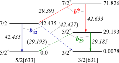
Figure 4: (color online). Relevant part of the level scheme of ²²⁹Th with transitions and branching ratios $b^{*}$, $b_{29}$, and $b_{42}$ used in the works Beck et al. (2007); Bec (b) to determine the energy of the isomeric level. Energies of the levels and transitions are given in keV.

Specifically, the authors showed that the value of the isomeric transition energy is shifted due to the unresolved transitions by Bec (b)

$$E_{is}=\frac{\Delta{}E_{29}-\Delta{}E_{42}}{1-b_{29}-b_{42}}\,,$$ (2)

where the branching ratio $b_{29}$ is given as Beck et al. (2007)

$$b_{29}=\frac{\Gamma_{rad}^{tot}(29.193\leavevmode\nobreak\ {\text{keV}})}{\Gamma_{rad}^{tot}(29.193\leavevmode\nobreak\ {\text{keV}})+\Gamma_{rad}^{tot}(29.185\leavevmode\nobreak\ {\text{keV}})}\,,$$ (3)

and the branching ratio $b_{42}$ is given as Bec (b)

$$b_{42}=\frac{\Gamma_{rad}^{tot}(42.427\leavevmode\nobreak\ {\text{keV}})}{\Gamma_{rad}^{tot}(42.427\leavevmode\nobreak\ {\text{keV}})+\Gamma_{rad}^{tot}(42.435\leavevmode\nobreak\ {\text{keV}})}\,.$$ (4)

In order to determine $b_{29}$, the authors of Ref. Beck et al. (2007) conducted additional measurements of the branching ratio

$$b^{*}=\frac{\Gamma_{rad}^{tot}(29.391\leavevmode\nobreak\ {\text{keV}})}{\Gamma_{rad}^{tot}(29.391\leavevmode\nobreak\ {\text{keV}})+\Gamma_{rad}^{tot}(42.633\leavevmode\nobreak\ {\text{keV}})}=\frac{1}{37}$$ (5)

with a quoted measurement accuracy of 8%. (Here, $\Gamma_{rad}^{tot}=\Gamma_{rad}(M1)+\Gamma_{rad}(E2)$ and the designations of the transition energies correspond to those in Fig. 4.) Using the Alaga rules (see Appendix B) the authors obtained $b_{29}\approx 1/13$. This led to the aforementioned increase of the energy of isomeric transition by 0.6 eV in accordance with the Eq. (2). In Ref. Bec (b), the authors performed an estimation of the value of the $b_{42}$ coefficient, which is several times smaller (see in Tab. 3) than $b_{29}$, leading to a smaller shift of 0.2 eV and the currently accepted value of $E_{is}=7.8\pm 0.5$ eV.

Interestingly, the same branching ratios can be obtained from the experimental data C. E. Bemis et al. (1988); Gulda et al. (2002); Barci et al. (2003); Ruchowska et al. (2006) for parameters of interband (see in Figure 1(a) and (b)) and inband transitions in the rotational bands $5/2^{+}[633]$ and $3/2^{+}[631]$ in the ²²⁹Th nucleus. The corresponding results are given in Table 3, where the probabilities of the inband transitions were calculated using the internal quadrupole moment $Q_{20}$ and the difference of the rotational and internal gyromagnetic ratio $g_{R}$ and $g_{K}$, respectively (for the rotational band $5/2^{+}[633]$ — $Q_{20}=7.1$ $e$b, $|g_{K}-g_{R}|=0.176$; for the rotational band $3/2^{+}[631]$ — $Q_{20}=7.1$ $e$b, $|g_{K}-g_{R}|=0.56$, (see Barci et al. (2003))).

Table 3: Branching ratios $b_{29}$ and $b_{42}$. Results are based on the data of the given references.

Ref.	Beck et al. (2007)	Bec (b)	C. E. Bemis et al. (1988)	Gulda et al. (2002)	Barci et al. (2003)	Ruchowska et al. (2006)
$b_{29}$	1/13		1/3.5	1/7.8	1/5.0	1/3.1
$b_{42}$		1/50	1/324	1/439	1/214	1/123

From Tab. 3, it is obvious that the branching ratios calculated by the Alaga rules show considerable spread. This fact is relatively unimportant for the coefficient $b_{42}$, as the relatively small value given in Bec (b) is the largest of the available in Table 3. Thus, if, for example, $b_{42}=1/439$ the isomeric transition energy would effectively shift back to the previous result of $E_{is}=7.6\pm 0.5$ eV Beck et al. (2007). The situation is more dramatic for the coefficient $b_{29}$. In the scenario $b_{29}\approx 1/3.1$, the energy of the isomer level would rise up to $\sim 10.5$ eV.

The data from Ref. Barci et al. (2003) allow for two additional estimates of the coefficient $b_{29}$. Specifically, Table VI of Ref. Barci et al. (2003) presents the intensities of gamma transitions from the levels $7/2^{+}(71.826$ keV) and $5/2^{+}(29.193$ keV); some of these data are experimental results, while others (namely, the relative intensities of the interband transitions) were calculated from the strong coupling rotational model. The branching ratios calculated from these data are presented in Tab. 4. In the case of the data for decays from the $7/2^{+}(71.826$ keV) level, we calculated the branching ratio $b_{29}$ by the formula (12) using the coefficient $b^{*}$.

Table 4: Coefficients $b^{*}$ and $b_{29}$ obtained from the data for the relative intensities of transitions in Barci et al. (2003).

Decaying level	$7/2^{+}(71.826$ keV)	$5/2^{+}(29.193$ keV)
$b^{*}$	1/17.5
$b_{29}$	1/6.4	1/3.9

These branching ratios are in rough agreement with those calculated for Tab. 3, but differ significantly from the measurement of Ref. Beck et al. (2007). The resolution of this tension between experiments is of the upmost importance. This can be seen by, for example, taking $b_{29}$ to be given by the statistical average of the values calculated here. In that case $b_{29}=1/5\pm 1/10$ and the isomeric transition energy becomes $E_{is}=9.3\pm 1.0$ eV. Despite this disagreement, we cannot reject the value of $b_{29}=1/13$ found in Ref. Beck et al. (2007), since $b^{*}$ is given directly from their experimental data and there is no proof this experiment, which used a state-of-the-art micro-calorimeter, is less reliable than the other measurements. Finally, we have performed Monte Carlo simulations of the Beck et al. experiments and if $b_{29}=1/3$, an asymmetry in the 29 keV peak should be visible. Unfortunately, the size of this asymmetry is smaller than be confirmed by simply viewing the presented date in Ref. Beck et al. (2007). In this regard, it would be interesting to reanalyze the experimental data.

VI Defining a favored area and current exclusions

Figure 5: (color online). Favored region and experimentally excluded regions for the nuclear isomeric transition as a function of transition energy (wavelength) and radiative lifetime. (Left) The favored region (dash-dotted blue line; see text) and currently accepted energy of the isomeric transition (dotted blue lines) according to Ref. Bec (a) are recommended as primary region of interest for current searches (blue shaded area). Experimentally excluded areas according to Ref. Moo (green shaded area between circles) and Ref. Jeet et al. (2015) (red shaded area between solid red lines) exclude parts of the favored region. Also shown are the more conservative bounds (outer dash-dotted yellow lines; see text). The point at 7.8 eV (blue circle) shows exemplarily the weighted average of the radiative lifetimes from reduced transition probabilities in Tab. 1 with 1.96 standard deviations including a Birge ratio of 3.4. (Right) Radiative lifetimes at 7.8 eV for individual values of the reduced transition probability with 1.96 standard deviations according to Tab. 1 (circles, blue) and Tab. 2 (squares, red). (The latter are only shown for completeness and do not enter into the construction of the favored region.)

As described in Sec. III, the measurements of Refs. C. E. Bemis et al. (1988); Gulda et al. (2002); Barci et al. (2003); Ruchowska et al. (2006) can be used to bound the isomeric level half life. In this section we will use the radiation lifetime instead of half-life, which is traditionally used in atomic spectroscopy. The radiative transition lifetime $\tau$ is bounded by (roughly 95% confidence level)

$$0.66\times 10^{6}\leavevmode\nobreak\ {\text{s\leavevmode\nobreak\ eV}}^{3}/\omega^{3}\leq\tau\leq 2.2\times 10^{6}\leavevmode\nobreak\ {\text{s\leavevmode\nobreak\ eV}}^{3}/\omega^{3}.$$

In Fig. 5, the bound is plotted as a function of isomeric transition energy (blue dash-dotted lines). For completeness, the energy ranges from 2.5 eV, which includes the now-rejected value of the transition energy from Ref. Helmer and Reich (1994) with one standard deviation towards lower energies, up to 10.5 eV, which is expected to be the largest possible value for the transition energy based on Sec. V. Further, the energy range for the currently accepted value of the transition energy of Ref. Bec (b) including two standard deviations is highlighted (see Fig. 5, blue dotted lines). The intersection of these two bounds, each at roughly the 95% confidence level, is marked as as blue shaded area and gives the primary region of interest. The energy and lifetime of the isomeric transition should be found at roughly the 90% confidence level in this region.

It is very likely that this region is somewhat conservative in its upper lifetime bound for two reasons. First, reduced transition probabilities calculated from the Alaga rules are typically smaller than actual values when the spin of the nucleus increases during the transition, as is the case here Casten (2000). Second, the measurements of the $B(M1;9/2^{+}5/2[633](97.14\leavevmode\nobreak\ {\text{keV}})\rightarrow 7/2^{+}3/2[631](71.83\leavevmode\nobreak\ {\text{keV}}))$ reduced transition probability rely on calculated values of the internal conversion coefficient, and there is evidence Tret’yakov et al. (1960) that these calculated internal conversion coefficients may lead to an underestimate of the reduced probabilities by a factor of $\sim 2$.

Also shown in Fig. 5, are the results from both an indirect Moo and direct Jeet et al. (2015) search for the low energy isomeric transition in the ²²⁹Th nucleus; a similar measurement to Moo was also performed by Kasamatsu et al. (2005). In Ref. Moo , ²²⁹Th produced in the $\alpha$ decay of ²³³U, with an estimated 2% of the ²²⁹Th populating the isomeric state, is chemically isolated from the ²³³U and any resulting fluorescence monitored with a photomultiplier tube. The initial photon count rate, based on a chi-squared analysis of binned photon counts, is then compared to what is expected from the known starting amount of ²³³U which then sets limits on the isomer lifetime. From these results, a 99.7% confidence interval can be constructed that excludes the possibility of the transition existing with a certain lifetime in a given energy range, as depicted by the green shading in Fig. 5.

In the recent direct search Jeet et al. (2015), tunable, broadband, synchrotron radiation is used to illuminate a ²²⁹Th⁴⁺ doped LiSrAlF₆ crystal. A photomultiplier tube is used to detect fluorescence subsequent to illumination of the crystal with the synchrotron beam. Applying a Feldman-Cousins analysis Feldman and Cousins (1998) to the binned photon counts, and comparing this to what is expected from experimental parameters, an exclusion region is created, depicted by the red shading between red solid lines in Fig. 5. This exclusion region represents a 90% confidence level for the absence of the isomeric transition.

VII Results, discussion, and request for future measurements

Even a cursory look at the results presented here reveals that the current situation is far from desirable. There is considerable scatter in the experimental data leading to a large range of predictions for the $3/2^{+}(7.8$ eV) ²²⁹Th isomer radiative lifetime. Likewise, though the basic value of $\Delta{}E_{29}-\Delta{}E_{42}=7.0\pm 0.5$  eV obtained in Beck et al. (2007) is not currently in question, there is significant spread in the braching ratio of two unresolved transitions, which systematically shift the value of the isomeric state.

Of course, the situation could be made much less ambiguous with an improved measurement of the intensities of the gamma transitions and internal conversion coefficients between the rotational bands $5/2^{+}[633]$ and $3/2^{+}[631]$ in the ²²⁹Th nucleus. Such an experiment would ideally resolve the tension between the current results of Ref. C. E. Bemis et al. (1988); Gulda et al. (2002); Barci et al. (2003); Ruchowska et al. (2006). This would allow accurate values of $b_{29}$ and $b_{42}$ to be calculated. Using these values in Eq. (2) and the value of $\Delta{}E_{29}-\Delta{}E_{42}=7.0\pm 0.5$ eV obtained in Beck et al. (2007), which so far is not in question, the isomeric state energy could be found with greater certainty. Further, these same experiments would give a definitive means to calculate the nuclear matrix element of the isomeric transition, and thus the radiative lifetime of the isomeric state.

Ideally, the measurements should be conducted for transitions from the rotational band $5/2^{+}[633]$ to the band $3/2^{+}[631]$, and vice versa, in the decay of states of the rotational band $3/2^{+}[631]$. Comparison of the data in Tables 1 and 2 indicates a systematic excess of the reduced probabilities obtained from the analysis of the decay data for the levels of the $5/2^{+}[633]$ rotational band. Reduced probabilities of interband transitions from the rotational band $3/2^{+}[631]$ to the band $5/2^{+}[633]$ are considerably less. This may indicate an error of measurements, as well as the inapplicability of the adiabatic approximation in the calculation using the Alaga rules.

If performed, these measurements would considerably sharpen the region of interest that must be scanned in the search for the isomeric transition. Given the challenges faced by these searches, this sharpening of the search space may prove to be a prerequisite for the completion of this decades old quest.

VIII Acknowledgement

This work has been supported in part by DARPA (QuASAR program), ARO (W911NF-11-1-0369), NSF (PHY-1205311), NIST PMG (60NANB14D302), and RCSA (20112810).

E.T. thanks the Russian government for its support of this work in the form of the salary of 22 thousand rubles per month (about $ 340) and Moscow State University, which adds to the salary monthly else 50% of the specified amount.

Appendix A Weisskopf Units

In modern nuclear spectroscopy a value of the reduced probability of transition between the nuclear states with the spins $I_{i}M_{i}$ and $I_{f}M_{f}$

$$\begin{split}B(E/ML;i\rightarrow{}f)&=\sum_{M_{f},M}|\langle{}I_{f}M_{f}|\hat{\cal{M}}^{E/M}_{LM}|I_{i}M_{i}\rangle|^{2}\\ &=\frac{|\langle{}I_{f}\|\hat{\cal{M}}^{E/M}_{L}\|I_{i}\rangle|^{2}}{2I_{i}+1}\,,\end{split}$$ (6)

where $\langle{}I_{f}\|\hat{\cal{M}}^{E/M}_{L}\|I_{i}\rangle$ is the reduced matrix element of the transition operator $\hat{\cal{M}}^{E/M}_{LM}$, usually is expressed in the Weisskopf units; see Eq. (1) and Ref. Bla . The nuclear wave functions are as a rule so complex that an exact calculation of the nuclear matrix elements becomes very difficult. The simplified single-particle Weisskopf model is convenient because it makes it easy to evaluate the nuclear matrix element of the electromagnetic transition. For this purpose the model uses the proton single-particle radial wave functions of the form $\varphi=\text{const.}$ inside the nucleus ($R\leq{}R_{0}$) and $\varphi(R)=0$ outside the nucleus ($R>R_{0}$). The normalization condition $\int_{0}^{R_{0}}|\varphi(R)|^{2}R^{2}dR=1$ gives $\text{const.}=\sqrt{3/R_{0}^{3}}$. Thus the total wave function of the proton has the form Bla

$$\Psi({\bf{R}})=\sqrt{\frac{3}{R_{0}^{3}}}Y_{LM}(\Omega_{\bf{R}})\chi_{1/2}\quad{\text{for}}\quad{}R\leq{}R_{0}\,,$$ (7)

where $\chi_{1/2}$ is the spin part, and $\Psi({\bf{R}})=0$ for $R>R_{0}$.

The radial part of the matrix element of the $EL$ proton transition operator $\hat{\cal{M}}^{E}_{LM}=eR^{L}Y_{LM}(\Omega)$ is easily calculated with the wave functions (7):

$$\langle\varphi_{f}(R)|R^{L}|\varphi_{i}(R)\rangle=\frac{3}{3+L}R_{0}^{L}\,.$$

From the angular part of the reduced matrix element in Eq. (6), $\langle{}f\|Y_{L}(\Omega)\|i\rangle$, only a factor $\sqrt{1/4\pi}$ is left, because $\sqrt{(2L_{i}+1)(2L+1)}C^{L_{f}0}_{L_{i}0L0}$ with the factor $1/\sqrt{(2I_{i}+1)}$ from (6) gives a value of about 1. (Here $C_{abcd}^{ef}$ is the Clebsch-Gordan coefficient Varshalovich et al. (1988).) As a result, the following expression is obtained in the Weisskopf model for the reduced probability of the $EL$ single-particle transition

$$\begin{split}B(W;EL)&=\frac{e^{2}}{4\pi}\left(\frac{3}{3+L}\right)^{2}R_{0}^{2L}\\ &=\frac{e^{2}}{4\pi}\left(\frac{3}{3+L}\right)^{2}1.2^{2L}A^{2L/3}\leavevmode\nobreak\ {\text{fm}}^{2L}.\end{split}$$

Here, the value of $R_{0}=1.2A^{1/3}$ fm was used for the radius of the nucleus with the atomic number $A$.

For the magnetic $ML$ transition the orbital ($l$) and the spin ($\sigma$) contributions leads to the relation

$$\frac{|\hat{\cal{M}}^{M}_{LM}(l)+\hat{\cal{M}}^{M}_{LM}(\sigma)|^{2}}{|\hat{\cal{M}}^{E}_{LM}|^{2}}\simeq\frac{10}{(M_{p}R_{0})^{2}}$$ (8)

between multipole moments of transition Bla . ($M_{p}$ in Eq. (8) is the proton mass.) This allows to write for the reduced probability of magnetic transitions in the Weisskopf model:

$$B(W;ML)=\frac{10}{(M_{p}R_{0})^{2}}B(W;EL).$$

Now, one can express the real reduced probability of a nuclear transition, $B(M/EL;i\rightarrow{}f)$, through the single particle reduced probability of the Weisskopf model $B(W;M/EL)$ according

$$B(E/ML;i\rightarrow{}f)=B(W;E/ML)B_{W.u.}(E/ML;i\rightarrow{}f)\,,$$

where $B_{W.u.}$ is the reduced probability in Weisskopf units, which is commonly used in tables of nuclear transitions.

The $\gamma$ emission probability in the Weisskopf model Bla

$$\Gamma_{rad}(W;E/ML)=\frac{8\pi}{[(2L+1)!!]^{2}}\frac{L+1}{L}\omega^{2L+1}B(W;E/ML)$$

satisfies the condition

$$\frac{\Gamma_{rad}(W;L+1)}{\Gamma_{rad}(W;L)}\sim(\omega{}R_{0})^{2}\sim\left(\frac{R_{0}}{\lambda}\right)^{2}$$

for the emission of $E(L+1)$ and $EL$ (or $M(L+1)$ and $ML$) multipoles. This approximation is true if the nuclear radius $R_{0}$ is small compared to the wavelength of nuclear transition $\lambda$. The latter condition is certainly satisfied for nuclear transitions with the energies up to several MeV.

Appendix B Branching Ratios

The section discussed the relation of the coefficients $b^{*}$ and $b_{29}$. Simple algebraic transformation of the Eq. (5) enables us to express the ratio of the widths of the transitions with energies of 42.627 keV and 29.391 keV through coefficient $b^{*}$:

$$\frac{\Gamma_{rad}^{tot}(42.627\leavevmode\nobreak\ {\text{keV}})}{\Gamma_{rad}^{tot}(29.391\leavevmode\nobreak\ {\text{keV}})}=\frac{1-b^{*}}{b^{*}}$$ (9)

Using the rotational model, we can express the radiation widths of the 29.185 keV transitions through the widths of the 42.627 keV transitions:

$$\Gamma_{rad}(M1;29.185\leavevmode\nobreak\ {\text{keV}})$$

$$\>=\left(\frac{C_{5/2\,3/2\,1\,0}^{3/2\,3/2}}{C_{7/2\,3/2\,1\,0}^{5/2\,3/2}}\right)^{2}\left(\frac{25.185}{42.627}\right)^{3}\times\Gamma_{rad}(M1;42.627\leavevmode\nobreak\ {\text{keV}})$$

$$\>=0.240\,\Gamma_{rad}(M1;42.627\leavevmode\nobreak\ {\text{keV}})$$

and

$$\Gamma_{rad}(E2;29.185\leavevmode\nobreak\ {\text{keV}})$$

$$\>=\left(\frac{C_{5/2\,3/2\,2\,0}^{3/2\,3/2}}{C_{7/2\,3/2\,2\,0}^{5/2\,3/2}}\right)^{2}\left(\frac{25.185}{42.627}\right)^{5}\times\Gamma_{rad}(E2;42.627\leavevmode\nobreak\ {\text{keV}})$$

$$\>=0.241\,\Gamma_{rad}(E2;42.627\leavevmode\nobreak\ {\text{keV}}).$$

Due to the coincidental equality of the transformation coefficients for the $M$1 and $E$2 components we obtain

$$\Gamma_{rad}^{tot}(29.185\leavevmode\nobreak\ {\text{keV}})=0.24\,\Gamma_{rad}^{tot}(42.627\leavevmode\nobreak\ {\text{keV}}).$$ (10)

Using the rotational model once again, we obtain the following relations:

$$\Gamma_{rad}(M1;29.193\leavevmode\nobreak\ {\text{keV}})=0.735\,\Gamma_{rad}(M1;29.391\leavevmode\nobreak\ {\text{keV}})$$

and

$$\Gamma_{rad}(E2;29.193\leavevmode\nobreak\ {\text{keV}})=1.36\,\Gamma_{rad}(E2;29.391\leavevmode\nobreak\ {\text{keV}}),$$

or, for the total linewidth,

$$\begin{split}\Gamma_{rad}^{tot}(29.193\leavevmode\nobreak\ {\text{keV}})&=0.735\,\left(\Gamma_{rad}^{tot}(29.391\leavevmode\nobreak\ {\text{keV}})\right.\\ &\quad+\left.0.85\,\Gamma_{rad}(E2;29.391\leavevmode\nobreak\ {\text{keV}})\right).\end{split}$$

Let us estimate the additional part $0.85\,\Gamma_{rad}(E2;29.391\leavevmode\nobreak\ {\text{keV}})$ to the width $\Gamma_{rad}^{tot}(29.391\leavevmode\nobreak\ {\text{keV}})$ using the mean values $B(M1)$ and $B(E2)$ for the interband transitions in Fig. 1 (a)–(b). The result is

$$\Gamma_{rad}(E2;29.391\leavevmode\nobreak\ {\text{keV}})\simeq 2\times 10^{-3}\,\Gamma_{rad}(M1;29.391\leavevmode\nobreak\ {\text{keV}}),$$

i.e. we really can neglect by the “extra” part $0.85\,\Gamma_{rad}(E2;29.391\leavevmode\nobreak\ {\text{keV}})$ in the width $\Gamma_{rad}^{tot}(29.391\leavevmode\nobreak\ {\text{keV}})$ and use the estimation

$$\Gamma_{rad}^{tot}(29.193\leavevmode\nobreak\ {\text{keV}})\approx 0.735\,\Gamma_{rad}^{tot}(29.391\leavevmode\nobreak\ {\text{keV}}).$$ (11)

Substituting expression (10), (11) and (9) in (3) we finally obtain

$$\begin{split}b_{29}&=\left(1+\frac{0.24\,\Gamma_{rad}^{tot}(42.627\leavevmode\nobreak\ {\text{keV}})}{0.735\,\Gamma_{rad}^{tot}(29.193\leavevmode\nobreak\ {\text{keV}})}\right)^{-1}\\ &=\left(1+\frac{0.24}{0.735}\frac{1-b^{*}}{b^{*}}\right)^{-1}.\end{split}$$ (12)

References

- Browne and Tuli (2008) E. Browne and J. K. Tuli, Nucl. Data Sheet 109, 2657 (2008).
- Jeet et al. (2015) J. Jeet, C. Schneider, S. T. Sullivan, W. G. Rellergert, S. Mirzadeh, A. Cassanho, H. P. Jenssen, E. V. Tkalya, and E. R. Hudson, Phys. Rev. Lett. 114, 253001 (2015).
- Strizhov and Tkalya (1991) V. F. Strizhov and E. V. Tkalya, Sov. Phys. JETP 72, 387 (1991).
- Porsev and Flambaum (2010a) S. G. Porsev and V. V. Flambaum, Phys. Rev. A 81, 032504 (2010a).
- Porsev and Flambaum (2010b) S. G. Porsev and V. V. Flambaum, Phys. Rev. A 81, 042516 (2010b).
- Dicke (1954) R. H. Dicke, Phys. Rev. 93, 99 (1954).
- Tkalya (2011) E. V. Tkalya, Phys. Rev. Lett. 106, 162501 (2011).
- Flambaum (2006) V. V. Flambaum, Phys. Rev. Lett. 97, 092502 (2006).
- He and Ren (2007) H.-t. He and Z.-z. Ren, J. Phys. G: Nucl. Phys. 34, 1611 (2007).
- Hayes and Friar (2007) A. C. Hayes and J. L. Friar, Phys. Lett. B 650, 229 (2007).
- Litvinova et al. (2009) E. Litvinova, H. Feldmeier, J. Dobaczewski, and V. Flambaum, Phys. Rev. C 79, 064303 (2009), URL http://link.aps.org/doi/10.1103/PhysRevC.79.064303.
- Dykhne and Tkalya (1998a) A. M. Dykhne and E. V. Tkalya, JETP Lett. 67, 549 (1998a).
- Dykhne et al. (1996) A. M. Dykhne, N. V. Eremin, and E. V. Tkalya, JETP Lett. 64, 345 (1996).
- Tkalya et al. (1996) E. V. Tkalya, V. O. Varlamov, V. V. Lomonosov, and S. A. Nikulin, Phys. Scr. 53, 296 (1996).
- Peik and Tamm (2000) E. Peik and C. Tamm, Europhys. Lett. 61, 181 (2000).
- Rellergert et al. (2010a) W. G. Rellergert, D. DeMille, R. R. Greco, M. P. Hehlen, J. R. Torgerson, and E. R. Hudson, Phys. Rev. Lett. 104, 200802 (2010a).
- Campbell et al. (2012) C. J. Campbell, A. G. Radnaev, A. Kuzmich, V. A. Dzuba, V. V. Flambaum, and A. Derevianko, Phys. Rev. Lett. 108, 120802 (2012).
- Peik and Okhapkin (2015) E. Peik and M. Okhapkin, C. R. Phys. 16, 516 (2015), ISSN 1631-0705, URL http://www.sciencedirect.com/science/article/pii/S1631070515000213.
- Burke et al. (2008) D. G. Burke, P. E. Garrett, T. Qu, and R. A. Naumann, Nucl. Phys. A 809, 129 (2008).
- Helmer and Reich (1994) R. G. Helmer and C. W. Reich, Phys. Rev. C 49, 1845 (1994).
- Guimaraes-Filho and Helene (2005) Z. O. Guimaraes-Filho and O. Helene, Phys. Rev. C 71, 044303 (2005).
- Beck et al. (2007) B. R. Beck, J. A. Becker, P. Beiersdorfer, G. V. Brown, K. J. Moody, J. B. Wilhelmy, F. S. Porter, C. A. Kilbourne, and R. L. Kelley, Phys. Rev. Lett. 98, 142501 (2007).
- Bec (a) B. R. Beck, C. Y. Wu, P. Beiersdorfer, G. V. Brown, J. A. Becker, J. K. Moody, J. B. Wilhelmy, F. S. Porter, C. A. Kilbourne, and R. L. Kelley, Lawrence Livermore National Laboratory, Conference LLNL-PROC-415170, 2009, URL http://www.osti.gov/scitech/biblio/964521-r2Qnkb/#.#.
- Zhao et al. (2012) X. Zhao, Y. N. M. de Escobar, R. Rundberg, E. M. Bond, A. Moody, and D. J. Vieira, Phys. Rev. Lett. 109, 160801 (2012).
- Tkalya (2000) E. V. Tkalya, JETP Lett. 71, 311 (2000).
- Tkalya et al. (2000) E. V. Tkalya, A. N. Zherikhin, and V. I. Zhudov, Phys. Rev. C 61, 064308 (2000).
- Kälber et al. (1989) W. Kälber, J. Rink, K. Bekk, W. Faubel, S. Göring, G. Meisel, H. Rebel, and R. Thompson, Z. Phys. A 334, 103 (1989), ISSN 0939-7922, URL http://dx.doi.org/10.1007/BF01294392.
- Campbell et al. (2009) C. J. Campbell, A. V. Steele, L. R. Churchill, M. V. DePalatis, D. E. Naylor, D. N. Matsukevich, A. Kuzmich, and M. S. Chapman, Phys. Rev. Lett. 102, 233004 (2009).
- Herrera-Sancho et al. (2012) O. A. Herrera-Sancho, M. V. Okhapkin, K. Zimmermann, C. Tamm, E. Peik, A. V. Taichenachev, V. I. Yudin, and P. Glowacki, Phys. Rev. A 85, 033402 (2012).
- Rellergert et al. (2010b) W. G. Rellergert, S. T. Sullivan, D. DeMille, R. R. Greco, M. P. Hehlen, R. A. Jackson, J. R. Torgerson, and E. R. Hudson, IOP Conf. Ser.: Mater. Sci. Eng. 15, 012005 (2010b).
- Hehlen et al. (2013) M. P. Hehlen, R. R. Greco, W. G. Rellergert, S. T. Sullivan, D. DeMille, R. A. Jackson, E. R. Hudson, and J. R. Torgerson, J. Lumin. 133, 91 (2013).
- Dessovic et al. (2014) P. Dessovic, P. Mohn, R. A. Jackson, J. Winkler, M. Schreitl, G. Kazakov, and T. Schumm, J. Phys.: Condens. Matter 26, 105402 (2014).
- Stellmer et al. (2015) S. Stellmer, M. Schreitl, and T. Schumm, arXiv 1506.01938, 1 (2015), eprint 1506.01938, URL http://arxiv.org/abs/1506.01938v1.
- Ellis et al. (2014) J. K. Ellis, X.-D. Wen, and R. L. Martin, Inorg. Chem. 53, 6769 (2014).
- Yamaguchi et al. (2015) A. Yamaguchi, M. Kolbe, H. Kaser, T. Reichel, A. Gottwald, and E. Peik, New J. Phys. 17, 053053 (2015).
- Okhapkin et al. (2015) M. V. Okhapkin, D. M. Meier, E. Peik, M. S. Safronova, M. G. Kozlov, and S. G. Porsev, Phys. Rev. A 92, 020503(R) (2015).
- Campbell et al. (2011) C. J. Campbell, A. G. Radnaev, and A. Kuzmich, Phys. Rev. Lett. 106, 223001 (2011).
- Radnaev et al. (2012) A. G. Radnaev, C. J. Campbell, and A. Kuzmich, Phys. Rev. A 44, 060501(R) (2012).
- Beloy (2014) K. Beloy, Phys. Rev. Lett. 112, 062503 (2014).
- Herrera-Sancho et al. (2013) O. A. Herrera-Sancho, N. Nemitz, M. V. Okhapkin, and E. Peik, Phys. Rev. A 88, 012512 (2013), URL http://link.aps.org/doi/10.1103/PhysRevA.88.012512.
- Bec (b) B. R. Beck and J. A. Becker and P. Beiersdorfer and G. V. Brown and K. J. Moody and J. B. Wilhelmy and F. S. Porter and C. A. Kilbourne and R. L. Kelley, Report LLNL-PROC-415170., URL https://e-reports-ext.llnl.gov/pdf/375773.pdf.
- Singh and Tuli (2005) B. Singh and J. K. Tuli, Nucl. Data Sheet 105, 109 (2005).
- (43) J. M. Blatt and V. F. Weisskopf, Theoretical Nuclear Physics. John Wiley & Sons, Inc. NY, 1952.
- Browne and Tuli (2013) E. Browne and J. K. Tuli, Nucl. Data Sheet 114, 751 (2013).
- Dykhne and Tkalya (1998b) A. M. Dykhne and E. V. Tkalya, JETP Lett. 67, 251 (1998b).
- C. E. Bemis et al. (1988) J. C. E. Bemis, F. K. McGowan, J. J. L. C. Ford, W. T. Milner, R. L. Robinson, P. H. Stelson, G. A. Leander, and C. W. Reich, Phys. Scr. 38, 657 (1988).
- Gulda et al. (2002) K. Gulda et al., (ISOLDE Collaboration), Nucl. Phys. A 703, 45 (2002).
- Barci et al. (2003) V. Barci, G. Ardisson, G. Barci-Funel, B. Weiss, O. El Samad, and R. K. Sheline, Phys. Rev. C 68, 034329 (2003).
- Ruchowska et al. (2006) E. Ruchowska, W. A. Plociennik, J. Zylicz, et al., Phys. Rev. C 73, 044326 (2006).
- Rikken and Kessener (1995) G. L. J. A. Rikken and Y. A. R. R. Kessener, Phys. Rev. Lett. 74, 880 (1995).
- Bodnar and Elster (2014) O. Bodnar and C. Elster, Metrologia 51, 516 (2014).
- Browne et al. (2001) E. Browne, E. B. Norman, R. D. Canaan, D. C. Glasgow, J. M. Keller, and J. P. Young, Phys. Rev. C 164, 014311 (2001).
- Kikunaga et al. (2009) H. Kikunaga, Y. Kasamatsu, H. Haba, T. Mitsugashira, M. Hara, K. Takamiya, T. Ohtsuki, A. Yokoyama, T. Nakanishi, and A. Shinohara, Phys. Rev. C 80, 034315 (2009), URL http://link.aps.org/doi/10.1103/PhysRevC.80.034315.
- Mitsugashira et al. (2003) T. Mitsugashira, M. Hara, T. Ohtsuki, H. Yuki, K. Takamiya, Y. Kasamatsu, A. Shinohara, H. Kikunaga, and T. Nakanishi, J. Radioanal. Nucl. Chem. 255, 63 (2003), ISSN 0236-5731, URL http://dx.doi.org/10.1023/A%3A1022267428310.
- Zimmermann (2010) K. Zimmermann, Dr. rer. nat., Gottfried Wilhelm Leibniz Universität Hannover (2010), URL http://edok01.tib.uni-hannover.de/edoks/e01dh10/634991264.pdf.
- Swanberg Jr. (2012) E. L. Swanberg Jr., Dissertation, University of California, Berkeley (2012), URL http://digitalassets.lib.berkeley.edu/etd/ucb/text/Swanberg_berkeley_0028E_12982.pdf.
- Utter et al. (1999) S. B. Utter, P. Beiersdorfer, A. Barnes, R. W. Lougheed, J. R. Crespo López-Urrutia, J. A. Becker, and M. S. Weiss, Phys. Rev. Lett. 82, 505 (1999), URL http://link.aps.org/doi/10.1103/PhysRevLett.82.505.
- Shaw et al. (1999) R. W. Shaw, J. P. Young, S. P. Cooper, and O. F. Webb, Phys. Rev. Lett. 82, 1109 (1999), URL http://link.aps.org/doi/10.1103/PhysRevLett.82.1109.
- (59) A. A. Soldatov and D. P. Grechukhin, Kourchatov Institute of Atomic Energy Report-3174, Moscow, 1979.
- Band and Fomichev (1979) I. M. Band and V. I. Fomichev, At. Data Nucl. Data Tabl. 23, 295 (1979).
- Nilsson (1955) S. G. Nilsson, Mat.-fys medd. danske selskab Bd. 29, n. 16 (1955).
- Church and Weneser (1956) E. L. Church and J. Weneser, Phys. Rev. 104, 1382 (1956).
- (63) M. E. Voikhansky, M. A. Listengarten, and I. M. Band, Penetration effects in internal conversion. In: Internal Conversion Processes, Ed. by J.H. Hamilton, Academic Press, NY, 1966, p.581.
- Tkalya (1994) E. V. Tkalya, JETP Lett. 78, 239 (1994).
- Reich and Helmer (1990) C. W. Reich and R. G. Helmer, Phys. Rev. Lett. 64, 271 (1990).
- (66) I. Moore, I. Ahmad, K. Bailey, D. L. Bowers, Z.-T. Lu, T. P. O’Connor, and Z. Yin, Argonne National Laboratory, Physics Division Report No. PHY-10990-ME-2004, 2004, URL http://www.phy.anl.gov/mep/atta/publications/thorium229_phy-10990-me-2004.pdf.
- Casten (2000) R. Casten, Nuclear Physics from a Simple Perspective (Oxford University Press, 2000).
- Tret’yakov et al. (1960) E. F. Tret’yakov, M. P. Anikina, L. L. Gol’din, G. I. Novikova, and N. I. Pirogova, Sov. Phys. JETP 37, 656 (1960).
- Kasamatsu et al. (2005) Y. Kasamatsu, H. Kikunaga, K. Nakashima, K. Takamiya, T. Mitsugashira, T. Nakanishi, T. Ohtsuki, H. Yuki, W. Sato, and A. Shinohara, Research Report vol. 38, p. 32–35, Laboratory of Nuclear Science, Tohoku University (2005), URL http://www.lns.tohoku.ac.jp/fy2011/research/report/2005/2005.htm.
- Feldman and Cousins (1998) G. J. Feldman and R. D. Cousins, Phys. Rev. D 57, 3873 (1998), URL http://link.aps.org/doi/10.1103/PhysRevD.57.3873.
- Varshalovich et al. (1988) D. A. Varshalovich, A. N. Moskalev, and V. K. Khersonslii, Quantum Theory of Angular Momentum (World Scientific Publ., London, 1988).