Massive stars exploding in a He-rich circumstellar medium - IX. SN 2014av, and characterization of Type Ibn SNe

Abstract

We present spectroscopic and photometric data of the Type Ibn supernova (SN) 2014av, discovered by the Xingming Observatory Sky Survey. Stringent pre-discovery detection limits indicate that the object was detected for the first time about 4 days after the explosion. A prompt follow-up campaign arranged by amateur astronomers allowed us to monitor the rising phase (lasting 10.6 days) and to accurately estimate the epoch of the maximum light, on 2014 April 23 (JD = 2456771.1 $\pm$ 1.2). The absolute magnitude of the SN at the maximum light is $M_{R}=-19.76\pm 0.16$. The post-peak light curve shows an initial fast decline lasting about 3 weeks, and is followed by a slower decline in all bands until the end of the monitoring campaign. The spectra are initially characterized by a hot continuum. Later on, the temperature declines and a number of lines become prominent mostly in emission. In particular, later spectra are dominated by strong and narrow emission features of He I typical of Type Ibn supernovae (SNe), although there is a clear signature of lines from heavier elements (in particular O I, Mg II and Ca II). A forest of relatively narrow Fe II lines is also detected showing P-Cygni profiles, with the absorption component blue-shifted by about 1200 km s^-1. Another spectral feature often observed in interacting SNe, a strong blue pseudo-continuum, is seen in our latest spectra of SN 2014av. We discuss in this paper the physical parameters of SN 2014av in the context of the Type Ibn supernova variety.

1 Introduction

Type Ibn SNe are a rare class of stripped-envelope events whose spectra usually show relatively narrow lines of He I along with broader lines of $\alpha$-elements similar to those observed in canonical Type Ib/c SNe (Pastorello et al., 2008a). The progenitors of SNe Ibn are thought to be hydrogen-poor Wolf-Rayet stars that have experienced major mass loss events shortly before the terminal SN explosions. A pre-SN outburst was directly observed in the case of the prototypical SN 2006jc (Pastorello et al., 2007; Foley et al., 2007). The variety of observed properties characterizing this SN family has been discussed by Turatto & Pastorello (2014), and several publications have been already devoted to this subject. However, although the number of Type Ibn SN discoveries is growing, very few objects boast well-sampled data sets, and only occasionally they were observed at early stages.

A rare opportunity to study a SN Ibn at very early phases has been provided with the discovery of a transient in the spiral galaxy UGC 4713, originally labelled as PSN J09002002+5229280, and later named with the IAU designation SN 2014av (Xu & Gao, 2014).

The new SN was discovered on 2014 April 19.72 UT (hereafter UT will be used along this paper), in the course of the Xingming Observatory Sky Survey (XOSS), at a magnitude of about 16.2 (Xu & Gao, 2014). The earliest pre-discovery detection of the transient was registered on April 16.84 UT on images of the Italian Supernovae Search Project (ISSP). Negative detections of the SN on images of UGC 4713 have been reported by the XOSS on March 26, 2014 and by the ISSP on April 6, 2014. These amateur observations allowed us to constrain the explosion epoch with a very little uncertainty to April 13, 2014 (see Section 2). The new SN exploded about 2”.7 West and 11”.2 South of the core of the host galaxy (see Figure 1), which is classified as Sb Type galaxy (from Hyperleda, Paturel et al., 2003). UGC 4713 has a recessional velocity corrected for Local Group infall into Virgo v_Vir = 9225 $\pm$ 12 km s^-1 (Mould et al., 2000, from the NASA/IPAC Extragalactic Database; NED). Adopting a value for the Hubble Constant H₀ = 73 km s^-1 Mpc^-1 and a standard cosmology ($\Omega_{M}$ = 0.27 and $\Omega_{\lambda}$ = 0.73), we obtain a luminosity distance $d=129\pm 9$ Mpc (hence, a distance modulus $\mu=35.56\pm 0.15$ mag). The Galactic extinction due to interstellar dust in the direction of SN 2014av is $A_{B}=0.062$ mag (Schlafly & Finkbeiner, 2011), and there are no spectroscopic signatures of additional reddening contribution in the host galaxy (cfr. Section 3).

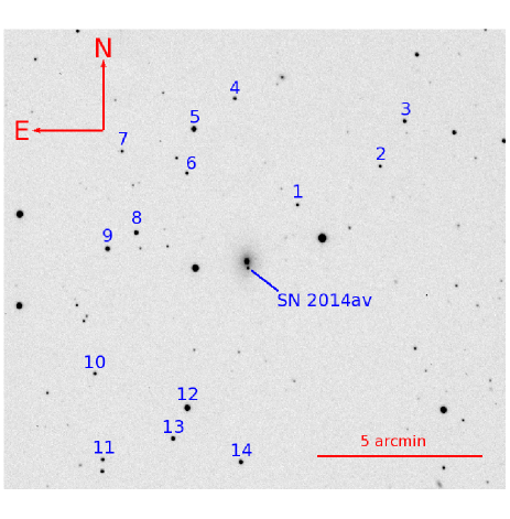
Figure 1: Unfiltered amateur image of the field of UGC 4713. SN 2014av and the 14 local sequence stars used for the photometric calibration are marked.

Table 1: Landolt-calibrated magnitudes of the reference stars in the field of UGC 4713, and associated errors.

Star ID	$R.A.$	$Dec.$	$U$	$B$	$V$	$R$	$I$
1	9:00:10.434	52:31:20.56	16.430 0.026	16.483 0.050	15.796 0.042	15.393 0.031	14.999 0.058
2	8:59:54.384	52:32:30.42	17.332 0.028	16.902 0.054	16.066 0.043	15.588 0.033	15.161 0.061
3	8:59:49.679	52:33:51.07	15.385 0.026	15.536 0.047	14.985 0.041	14.662 0.029	14.341 0.051
4	9:00:22.854	52:34:28.95	16.052 0.019	16.164 0.038	15.583 0.028	15.245 0.028	14.917 0.052
5	9:00:30.755	52:33:33.87	14.516 0.018	14.339 0.040	13.695 0.027	13.309 0.028	12.899 0.054
6	9:00:32.061	52:32:15.37	16.441 0.020	16.419 0.041	15.742 0.028	15.350 0.030	14.983 0.055
7	9:00:44.747	52:32:53.21	17.259 0.022	16.961 0.046	16.117 0.030	15.634 0.033	15.200 0.062
8	9:00:41.823	52:30:28.80	15.266 0.029	15.037 0.043	14.386 0.033	14.008 0.031	13.646 0.051
9	9:00:47.372	52:29:59.52	14.555 0.028	14.622 0.040	14.095 0.032	13.828 0.028	13.680 0.044
10	9:00:49.557	52:26:17.28	17.943 0.033	16.941 0.059	15.805 0.038	15.142 0.045	14.518 0.086
11	9:00:47.894	52:23:44.54	16.140 0.029	16.051 0.041	15.465 0.032	15.114 0.031	14.745 0.052
12	9:00:31.525	52:25:17.66	13.652 0.028	13.491 0.032	12.916 0.015	12.578 0.025	12.240 0.047
13	9:00:34.258	52:24:22.86	17.542 0.031	16.393 0.066	15.092 0.041	14.328 0.052	13.607 0.101
14	9:00:21.035	52:23:42.40	15.557 0.029	15.328 0.044	14.614 0.033	14.185 0.035	13.737 0.061

Zhang & Wang (2014), on the basis of the blue spectral continuum and a presence of relatively narrow He I lines, classified SN 2014av as a young Type Ibn SN similar to SN 2006jc. The young age of the SN and the rarity of Type Ibn events ($\leq$ 2 per cent of core-collapse SNe, Pastorello et al., 2015a) motivated our team to initiate a monitoring campaign of this new member of the family. Photometric and spectroscopic observations of SN 2014av are presented in Sections 2 and 3, respectively; a bolometric light curve and an estimate of the explosion parameters are given in Section 4. An extensive characterization of spectral properties of SNe Ibn is provided in Section 5. The properties of the progeniors of SNe Ibn are illustrated in Section 6 and a summary follows in Section 7.

2 Photometric Observations

Our multi-band (Johnson-Cousins $UBVRI$ and Sloan $griz$) photometric follow-up campaign started when the object had already reached the maximum light, and continued up to phase $\sim$70 days after discovery, until the object became unobservable because it was in solar conjunction. The instruments used in our photometric campaign are the 3.58-m Telescopio Nazionale Galileo (TNG) equipped with Dolores, the 2.56-m Nordic Optical Telescope (NOT) with ALFOSC and the 2.0-m Liverpool Telescope with IO:O, all located at Roque de los Muchachos Observatory, La Palma, Canary Islands (Spain); the 1.82-m Copernico Telescope of Mt. Ekar, Asiago (Italy) equipped with AFOSC. In order to sample the early-time SN evolution, we included in our dataset unfiltered observations from amateur astronomers. The instruments used are listed as a footnote in the SN photometry tables. These additional data, essential to constrain the rising branch of the light curve and the peak luminosity, were scaled to $V$ or $R$-band (and similarly to Sloan $g$ or $r$-band) photometry, depending on the approximate wavelength of the peak of the quantum efficiency curves of the CCDs used in the observations.

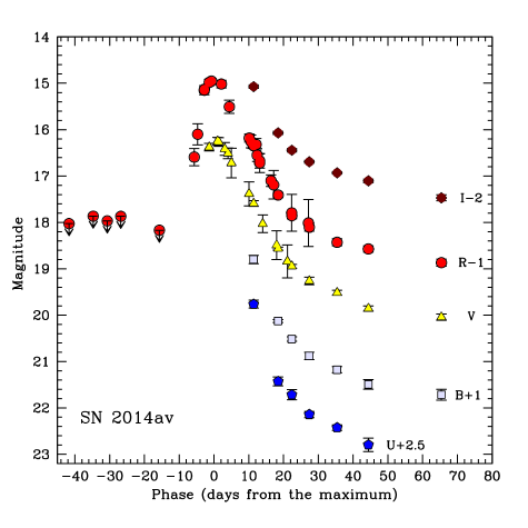
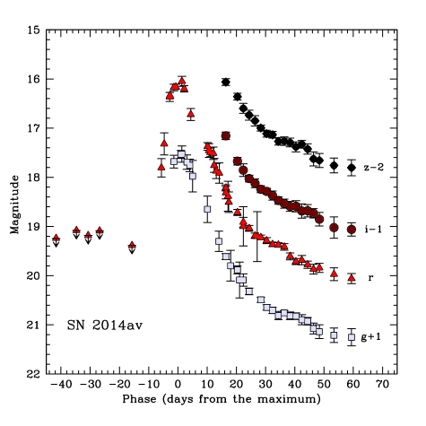
Figure 2: $UBVRI$ (left) and $griz$ (right) light curves of SN 2014av. The closest pre-discovery limits are also shown. Data from unfiltered images are rescaled to Johnson-Cousins $V$ or $R$ (vegamag), and Sloan $g$ or $r$ (ABmag), depending on the wavelength of the peak of the quantum efficiency curves of the CCDs used for the observations, as specified in the text.

All frames were pre-processed using standard procedures in IRAF. We corrected the frames for bias, overscan and flat-fielding, and they were finally astrometrically calibrated. For photometric measurements, we used the dedicated pipeline SNOoPY (Cappellaro, 2014). This pipeline consists of a collection of PYTHON scripts calling standard IRAF tasks, and other data analysis tools such as SEXTRACTOR for source extraction and classification, DAOPHOT for point spread function (PSF) fitting, and HOTPANTS for PSF matching and image subtraction. PSF-fitting photometry provided reliable results in the high-quality, high signal-to-noise (S/N) filtered images from professional telescopes, whilst this measurement method provided inaccurate results in lower S/N unfiltered images from amateur astronomers. For the latter epochs, we employed the template subtraction method to remove the contaminating flux from the host galaxy background. Good-quality pre-explosion images of UGC 4713 were used as templates. These images were available after the routine monitoring observations of UGC 4713 obtained in the course of the XOSS and ISSP SN searches.

Table 2: Johnson-Cousins magnitudes of SN 2014av, and associated errors.

Obs. date	Average $JD$	$U$	$B$	$V$	$R$	$I$	Instrument
2010/03/14	2455270.39	–	–	–	$>$19.26	–	1
2011/03/09	2455630.37	–	–	–	$>$19.27	–	1
2013/12/03	2456630.49	–	–	–	$>$18.93	–	1
2013/12/10	2456637.58	–	–	–	$>$19.19	–	1
2013/12/19	2456645.55	–	–	–	$>$19.17	–	1
2014/01/06	2456664.49	–	–	–	$>$18.52	–	1
2014/03/11	2456728.33	–	–	–	$>$19.03	–	1
2014/03/18	2456735.29	–	–	–	$>$18.87	–	1
2014/03/22	2456739.32	–	–	–	$>$18.97	–	2
2014/03/26	2456743.23	–	–	–	$>$18.87	–	2
2014/04/06	2456754.31	–	–	–	$>$19.17	–	1
2014/04/16	2456764.34	–	–	–	17.592 0.185	–	1
2014/04/17	2456765.32	–	–	–	17.100 0.229	–	1
2014/04/19	2456767.22	–	–	–	16.150 0.098	–	2
2014/04/19	2456767.27	–	–	–	16.130 0.079	–	2
2014/04/21	2456768.63	–	–	16.379 0.080	15.983 0.067	–	3
2014/04/21	2456769.28	–	–	–	15.954 0.058	–	4
2014/04/23	2456771.03	–	–	16.253 0.083	–	–	5
2014/04/23	2456771.38	–	–	16.266 0.094	–	–	6
2014/04/24	2456772.14	–	–	–	16.018 0.083	–	2
2014/04/25	2456773.09	–	–	16.417 0.138	–	–	5
2014/04/26	2456774.04	–	–	16.512 0.114	–	–	5
2014/04/26	2456774.41	–	–	–	16.507 0.143	–	1
2014/04/27	2456775.02	–	–	16.720 0.320	–	–	5
2014/05/02	2456780.10	–	–	17.383 0.260	–	–	5
2014/05/02	2456780.16	–	–	–	17.182 0.087	–	2
2014/05/03	2456780.63	–	–	–	17.254 0.139	–	7
2014/05/03	2456781.14	–	–	–	17.311 0.086	–	2
2014/05/03	2456781.41	17.263 0.087	17.800 0.090	17.592 0.063	17.348 0.033	17.073 0.037	8
2014/05/04	2456782.13	–	–	–	17.320 0.126	–	2
2014/05/04	2456782.42	–	–	–	17.549 0.140	–	9
2014/05/05	2456783.14	–	–	–	17.676 0.153	–	2
2014/05/06	2456784.03	–	–	18.031 0.191	–	–	5
2014/05/06	2456784.15	–	–	–	17.720 0.204	–	2
2014/05/08	2456786.40	–	–	–	18.101 0.125	–	1
2014/05/09	2456787.16	–	–	–	18.191 0.307	–	2
2014/05/10	2456788.02	–	–	18.491 0.309	–	–	5
2014/05/10	2456788.45	18.928 0.097	19.125 0.030	18.566 0.031	18.410 0.051	18.071 0.034	10
2014/05/13	2456791.10	–	–	18.841 0.354	–	–	5
2014/05/14	2456792.36	–	–	–	18.794 0.397	–	1
2014/05/14	2456792.39	19.215 0.109	19.515 0.047	18.946 0.043	18.856 0.069	18.444 0.039	8
2014/05/19	2456797.16	–	–	–	19.012 0.507	–	2
2014/05/19	2456797.41	19.641 0.067	19.877 0.078	19.263 0.081	19.104 0.089	18.694 0.030	8
2014/05/27	2456805.40	19.924 0.059	20.177 0.066	19.518 0.056	19.430 0.075	18.931 0.027	8
2014/06/05	2456814.39	20.296 0.145	20.492 0.101	19.857 0.056	19.573 0.068	19.105 0.038	8
2014/06/26	2456835.39	–	20.715 0.116	20.043 0.065	19.869 0.076	19.471 0.064	8

1 = 0.50-m Newton telescope (Lotti) + FLI Proline 4710 CCD (ISSP collaboration, Osservatorio Astronomico di Monte Agliale, Borgo a Mozzano, Lucca, Italy); 2 = 0.36-m Celestron C14 telescope + QHY9 + KAF8300 CCD (Obs. Z. Xu $\&$ X. Gao, Xingming Observatory; Xiaofeng, Gangou, China); 3 = 0.36-m Celestron C14 telescope + DSI Pro-DSI ll CCD (Obs. W. S. Wiethoff; SOLO Observatory, Port Wing, Wisconsin, USA); 4 = 0.43-m Planewave Corrected Dall-Kirkham Astrograph + Paramount ME + SBIG STL-6303E CCD (Obs. G. Masi, The Virtual Telescope Project 2.0, Bellatrix Astronomical Observatory, Ceccano, Frosinone, Italy); 5 = 0.25-m Whitey Dob telescope + Starlight Xpress SXVR-H694 CCD (Obs. S. Tokuoka, Takatsuki, Osaka, Japan); 6 = 0.25-m Meade SC telescope + Atik 314L+ Sony ICX-285AL CCD (Obs. G. Locatelli; Maritime Alps Observatory MPC K32, Cuneo, Italy); 7 = 0.28-m Celestron C11 telescope + Orion StarShoot DSMI III CCD (Obs. S. Howerton; Arkansas City, Kansas, USA); 8 = 3.58-m TNG + Dolores (Roque de los Muchachos, La Palma, Canary Islands, Spain); 9 = 0.28-m Celestron C11 telescope + SBIG STT-1603 ME camera (Obs. J.-M. Llapasset; Perpignan Observatory, France); 10 = 2.56-m NOT + ALFOSC (Roque de los Muchachos, La Palma, Canary Islands, Spain).

Table 3: Sloan magnitudes of SN 2014av, and associated errors.

Obs. date	Average $JD$	$g$	$r$	$i$	$z$	Instrument
2010/03/14	55270.390	–	$>$19.48	–	–	1
2011/03/09	55630.374	–	$>$19.47	–	–	1
2013/12/03	56630.490	–	$>$19.15	–	–	1
2013/12/10	56637.581	–	$>$19.38	–	–	1
2013/12/19	56645.553	–	$>$19.39	–	–	1
2014/01/06	56664.491	–	$>$18.70	–	–	1
2014/03/11	56728.331	–	$>$19.24	–	–	1
2014/03/18	56735.287	–	$>$19.08	–	–	1
2014/03/22	56739.318	–	$>$19.18	–	–	2
2014/03/26	56743.226	–	$>$19.09	–	–	2
2014/04/06	56754.313	–	$>$19.39	–	–	1
2014/04/16	56764.341	–	17.808 0.187	–	–	1
2014/04/17	56765.316	–	17.321 0.224	–	–	1
2014/04/19	56767.217	–	16.365 0.092	–	–	2
2014/04/19	56767.267	–	16.337 0.059	–	–	2
2014/04/21	56768.632	16.681 0.131	16.174 0.066	–	–	3
2014/04/21	56769.284	–	16.162 0.053	–	–	4
2014/04/23	56771.030	16.534 0.080	–	–	–	5
2014/04/23	56771.381	16.529 0.165	16.049 0.100	–	–	6
2014/04/24	56772.138	–	16.201 0.065	–	–	2
2014/04/25	56773.089	16.690 0.147	–	–	–	5
2014/04/26	56774.042	16.758 0.125	–	–	–	5
2014/04/26	56774.413	–	16.723 0.121	–	–	1
2014/04/27	56775.024	16.978 0.320	–	–	–	5
2014/05/02	56780.099	17.652 0.270	–	–	–	5
2014/05/02	56780.158	–	17.373 0.077	–	–	2
2014/05/03	56780.632	–	17.455 0.140	–	–	7
2014/05/03	56781.136	–	17.495 0.087	–	–	2
2014/05/04	56782.131	–	17.512 0.127	–	–	2
2014/05/04	56782.417	–	17.759 0.141	–	–	8
2014/05/05	56783.143	–	17.872 0.155	–	–	2
2014/05/06	56784.031	18.301 0.205	–	–	–	5
2014/05/06	56784.153	–	17.915 0.206	–	–	2
2014/05/08	56786.385	18.613 0.061	18.215 0.062	18.157 0.075	18.064 0.068	9
2014/05/08	56786.404	–	18.313 0.127	–	–	1
2014/05/09	56787.158	–	18.385 0.305	–	–	2
2014/05/09	56787.407	–	18.505 0.208	–	–	10
2014/05/10	56788.023	18.797 0.312	–	–	–	5
2014/05/12	56790.370	18.883 0.082	18.714 0.062	18.673 0.078	18.361 0.068	9
2014/05/13	56791.096	19.089 0.363	–	–	–	5
2014/05/14	56792.361	–	18.998 0.398	–	–	1
2014/05/14	56792.370	19.088 0.124	18.911 0.095	18.855 0.128	18.599 0.103	9
2014/05/16	56794.370	19.321 0.067	19.038 0.059	19.027 0.068	18.736 0.101	9
2014/05/18	56796.385	–	19.189 0.053	19.122 0.090	18.852 0.106	9
2014/05/09	56797.159	–	19.206 0.506	–	–	2
2014/05/20	56798.380	19.490 0.053	19.222 0.048	19.242 0.070	18.998 0.060	9
2014/05/22	56800.375	19.646 0.056	19.288 0.061	19.286 0.060	19.114 0.068	9
2014/05/24	56802.380	19.706 0.065	19.363 0.048	19.373 0.092	19.136 0.068	9
2014/05/26	56804.380	19.811 0.084	19.376 0.046	19.470 0.076	19.270 0.076	9
2014/05/28	56806.395	19.754 0.045	19.414 0.067	19.534 0.092	19.265 0.087	9
2014/05/30	56808.385	19.817 0.078	19.606 0.070	19.591 0.100	19.294 0.089	9
2014/06/01	56810.385	19.823 0.066	19.715 0.061	19.589 0.114	19.381 0.101	9
2014/06/03	56812.390	19.896 0.103	19.685 0.093	19.686 0.144	19.328 0.077	9
2014/06/05	56814.385	19.927 0.075	19.777 0.073	19.680 0.126	19.426 0.105	9
2014/06/07	56816.385	20.074 0.110	19.867 0.099	19.732 0.094	19.626 0.144	9
2014/06/09	56818.390	20.138 0.139	19.843 0.092	19.852 0.138	19.657 0.143	9
2014/06/14	56823.395	20.212 0.147	19.971 0.131	20.022 0.216	19.759 0.150	9
2014/06/20	56829.390	20.253 0.173	20.059 0.104	20.060 0.137	19.805 0.162	9

1 = 0.51-m Lotti telescope + FLI Proline 4710 CCD (ISSP collaboration, Osservatorio di Monte Agliale, Borgo a Mozzano, Lucca, Italy); 2 = 0.36-m Celestron C14 telescope + QHY9 + KAF8300 CCD (Obs. Z. Xu $\&$ X. Gao, Xingming Observatory; Xiaofeng, Gangou, China); 3 = 0.36-m Celestron C14 telescope + DSI Pro-DSI ll CCD (Obs. W. S. Wiethoff; SOLO Observatory, Port Wing, Wisconsin, USA); 4 = 0.43-m Planewave Corrected Dall-Kirkham Astrograph + Paramount ME + SBIG STL-6303E CCD (Obs. G. Masi, The Virtual Telescope Project 2.0, Bellatrix Astronomical Observatory, Ceccano, Frosinone, Italy); 5 = 0.25-m Whitey Dob telescope + Starlight Xpress SXVR-H694 CCD (Obs. S. Tokuoka, Takatsuki, Osaka, Japan); 6 = 0.25-m Meade SC telescope + Atik 314L + Sony ICX-285AL CCD (Obs. G. Locatelli; Maritime Alps Observatory MPC K32, Cuneo, Italy); 7 = 0.28-m Celestron C11 telescope + Orion StarShoot DSMI III CCD (Obs. S. Howerton; Arkansas City, Kansas, USA); 8 = 0.28-m Celestron C11 telescope + SBIG STT-1603 ME camera (Obs. J.-M. Llapasset; Perpignan Observatory, France); 9 = 2.0-m Liverpool Telescope + IO:O camera (Roque de los Muchachos, La Palma, Canary Islands, Spain); 10 = 1.82-m Copernico Telescope (Mt. Ekar, Asiago Observatory, Italy).

Table 4: Main light curve parameters for SN 2014av.

Filter	peak magnitude	$\gamma_{0-25}^{\ddagger}$	$\gamma_{25-60}^{\ddagger}$
$U$	–	18.47 $\pm$ 4.24	3.86 $\pm$ 0.17
$B$	–	16.00 $\pm$ 2.32	2.12 $\pm$ 0.49
$V$	16.24$\pm$0.07	13.40 $\pm$ 0.26	2.00 $\pm$ 0.50
$R$	15.85$\pm$0.05	12.73 $\pm$ 0.55	1.87 $\pm$ 0.36
$I$	–	12.69 $\pm$ 1.22	1.98 $\pm$ 0.17
$g$	16.52$\pm$0.04	13.11 $\pm$ 0.46	2.63 $\pm$ 0.21
$r$	16.07$\pm$0.05	12.98 $\pm$ 0.46	3.07 $\pm$ 0.12
$i$	–	11.85 $\pm$ 0.95	2.84 $\pm$ 0.17
$z$	–	8.61 $\pm$ 0.58	2.93 $\pm$ 0.22

^‡ in mag/100^d units

Once instrumental magnitudes of the SN and a number of stellar sources in the SN vicinity were obtained, we accurately calibrated the Johnson-Cousins magnitudes of a sequence of local standards in the field. To this aim, we selected observations obtained during a few photometric nights in which standard photometric fields from the catalogue of Landolt (1992) were also observed. These observations allowed us to obtain the zero-points and colour terms for each night and each specific instrumental set-up. The resulting calibrated magnitudes of the sequence stars in the SN field were derived by averaging the measures obtained during these selected nights (see Figure 1 and Table 1). This allowed us to correct the zero-points estimated in non photometric nights and accurately calibrate the SN magnitudes. Sloan-band photometry was directly calibrated using the SDSS DR10 catalogue. The final Johnson-Cousins and Sloan magnitudes of the SN are reported in Table 2 and Table 3, respectively, and the resulting light curves are shown in Figure 2.

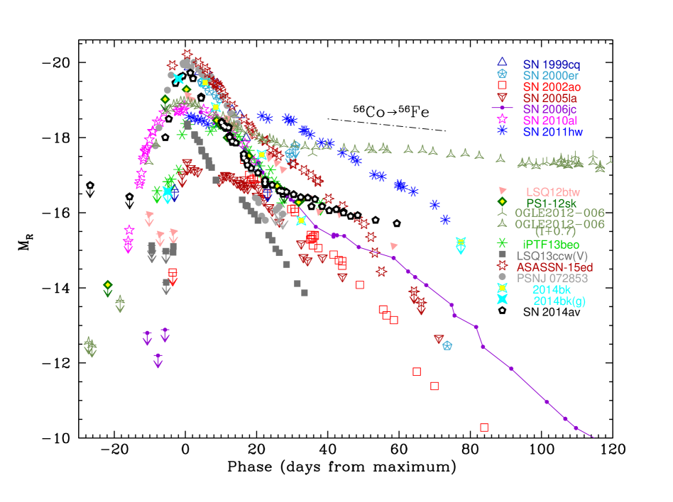
Figure 3: $R$-band absolute light curves of SN 2014av and a wide sample of SNe Ibn (for the sources of the data, see notes underneath Table 5). The most significant pre-discovery limits are also shown. For OGLE-2012-SN-006, along with the poorly sampled $R$-band light curve, the $I$-band light curve is also shown for completeness, scaled by $+$0.7 mag to approximately match the $R$-band points. For LSQ13ccw, we showed the best sampled $V$-band light curve. SN 2014bk, whose data are shown here for the first time, is poorly sampled in the R band. For this reason, we also report the closest detection limit of SN 2014bk and the $g$-band discovery magnitude announced in Morokuma et al. (2014).

Thanks to the data collected by amateur astronomers, we were able to monitor the light curve rising phase, hence to provide an estimate of the explosion epoch. Through a low-order polynomial fit, we found that the $R$-band maximum occurred on 2014 April 23.6 UT ($JD$ = 2456771.1 $\pm$ 1.2). Fitting the earliest photometric data using a parabolic function, we estimated that the explosion occurred 10.6 days before maximum, i.e. on $JD$ = 2456760.5, which is fully consistent with the epoch suggested by the latest non-detection on 2014 April 6.8 UT ($JD$ = 2456754.3).

Table 5: Main light-curve parameters for our sample of Type Ibn SNe, including absolute peak magnitudes (column 5), rise-time to the $R$-band maximum (column 6), and decline rates at three different time intervals (columns 7 to 9). Information on the reddening is provided in the reference papers; when not available, the Milky Way component is taken from Schlafly & Finkbeiner (2011), while the host galaxy component is obtained by measuring the equivalent width of the interstellar Na I doublet lines from the low resolution spectra available to us, adopting the low-reddening empirical relation from Turatto et al. (2003). The slopes are measured in units of mag 100$d^{-1}$.

SN	Type	$\mu$	$E(B-V)_{tot}$	$M_{R,peak}$	Rise time (d)	$\gamma^{R}_{0-25}$	$\gamma^{R}_{25-60}$	$\gamma^{R}_{60-150}$	Sources
SN 1999cq	Ibn	35.27	0.15	$-$19.87	$<$4	15.5$\pm$1.9	–	–	1
SN 2000er	Ibn	35.52	0.11	$<-$19.49	–	8.9$\pm$0.6	–	–	2
SN 2002ao	Ibn	31.73	0.25	$<-$17.41	–	12.6$\pm$2.5	9.8$\pm$0.3	–	2
SN 2005la	Ibn/IIn	34.49	0.01	$-$17.19	–	non-monotonic	7.5$\pm$0.6	–	3
SN 2006jc	Ibn	32.01	0.04	$<-$18.61‡	$<$10	8.6$\pm$0.7	7.7$\pm$0.3	7.9$\pm$0.2	3,4,5
SN 2010al	Ibn	34.27	0.06	$-$18.86	16	9.4$\pm$0.6	12.6$\pm$0.2	–	8
SN 2011hw	Ibn/IIn	34.92	0.10	$<-$18.54	–	non-monotonic	5.5$\pm$0.1	–	8
PS1-12sk	Ibn	36.84	0.03	$-$19.21	$<$23	10.8$\pm$0.9	–	–	9
OGLE-006⋆	Ibn	36.94	0.07	$-$19.65	15.6	4.8$\pm$0.1	0.4$\pm$0.1	1.0$\pm$0.1	10
LSQ12btw	Ibn	36.97	0.02	$-$19.14	$<$4	7.3$\pm$0.4	5.8$\pm$0.7	–	11
iPTF13beo	Ibn-pec	38.01	0.04	$-$18.39	–	non-monotonic	12.8$\pm$3.5	–	12
LSQ13ccw⊙	Ibn-pec	37.07	0.04	$-$18.36	$<$6	12.6$\pm$0.2	$\sim$15.5	–	11
CSS140421†	Ibn	37.41	0.03:	$-$19.4:	–	–	–	–	13
ASASSN-14dd⊙	Ibn	34.23	0.15:	$-$19.1:	–	–	–	–	14
SN 2014av∗	Ibn	35.56	0.02	$-$19.75	10.6	12.1$\pm$0.7∗	3.0$\pm$0.2∗	–	15
SN 2014bk	Ibn	37.40	0.05	$<-$19.47	–	13.1$\pm$1.1	–	–	15
ASASSN-15ed	Ibn/Ib	36.59	0.14	$-$20.19	–	11.4 $\pm$ 0.2	7.7 $\pm$ 0.3	26.3 $\pm$ 2.5	16
PSN J07285387+3349106	Ibn	33.85	1.02	$-$19.95♢	$>$8.7	19.7$\pm$1.6	–	–	17
SN 2015G	Ibn/Ib	31.80	0.33:	$<-$17.1	–	–	–	–	18

^⋆ OGLE-006 = OGLE-2012-SN-006 ($I$-band light curve data). ^† CSS140421 = CSS140421:142042+031602. ^‡ From unpublished data kindly provided by K. Itagaki. ^⊙ For LSQ13ccw, we considered the $V$-band light curve information; for ASASSN-14dd, we considered the $V$-band discovery magnitude. ^∗ Average between the $R$- and $r$-band slopes. ^♢ The uncertainty in the line-of-sight reddening to PSN J07285387+3349106 is extremely large, giving an error in the $R$-band absolute magnitude of $\pm$1.13 mag.

1 = Matheson et al. (2000); 2 = Pastorello et al. (2008a); 3 = Pastorello et al. (2008b); 4 = Pastorello et al. (2007); 5 = Foley et al. (2007); 8 = Pastorello et al. (2015b); 9 = Sanders et al. (2013); 10 = Pastorello et al. (2015c); 11 = Pastorello et al. (2015a); 12 = Gorbikov et al. (2014); 13 = Polshaw et al. (2014); 14 = Stanek et al. (2014); 15 = this paper; 16 = Pastorello et al. (2015d); 17 = Pastorello et al. (2015e); 18 = Yusa et al. (2015).

Using low-order polynomial fits, we also estimated the peak magnitude and the decline rate of SN 2014av in the different bands. As there is a clear change in the slope of the light curves of SN 2014av at $\sim$ 25 days after maximum, we computed the SN magnitude decline rates in two time intervals: from the peak to 25 days after maximum, and from 25 days to the latest detections. The results are reported in Table 4. We note, in particular, that the blue-band light curves decline faster than the red-band light curves. This trend is more evident during the early decline ($\gamma_{0-25}$ in Table 4), while at later phases there is more homogeneity in the decline rates. The decline rates in all bands during the temporal window 25-60 days ($\gamma_{25-60}$) are much faster than those expected from the decay of ⁵⁶Co into ⁵⁶Fe. However, as we will discuss later in this paper, other indicators suggest that during the entire monitoring period, the radioactive decays are not the major powering source for the light curve of SN 2014av (see Section 4).

Additional near-infrared (NIR) photometry was obtained on 2014 May 16 (i.e. one month after the SN discovery) at the TNG, equipped with NICS. The images were reduced following standard prescriptions, including flat-field correction and sky subtraction; individual dithered images for each band were then combined to obtain a single, higher S/N frame. The observations, calibrated using the 2MASS catalogue (Skrutskie et al., 2006), provided the following photometric measurements: $J$ = 18.33 $\pm$ 0.06, $J-H$ = 0.29 $\pm$ 0.07 and $J-K$ = 0.74 $\pm$ 0.13. We can note that, at this epoch, there is no signature of a significant NIR flux excess.

2.1 Absolute light curve

Table 6: Log of spectroscopic observations of SN 2014av.

Obs. date	Average JD	Days	Instrumental configuration	Exposure time	Range	Resolution
	(+2400000)	(after maximum)		(s)	(Å)	(Å)
2014/04/23	56771.14	0	Lijiang 2.4m telescope + YFOSC + gm10	600	3560–9160	45
2014/05/01	56779.04	7.9	Lijiang 2.4m telescope + YFOSC + gm10	1200	3460–9250	45
2014/05/03	56781.37	10.3	3.58m TNG + Dolores + LRB + LRR	2400+1200	3250-10000	11;10
2014/05/04	56782.11	11.0	Lijiang 2.4m telescope + YFOSC + gm10	1238	4040–9270	45
2014/05/10	56788.49	17.4	2.56m NOT + ALFOSC + gm4	2$\times$2700	3400–9090	18
2014/05/19	56797.46	26.4	3.58m TNG + Dolores + LRR	2700	5020–9740	14
2014/05/27	56805.44	34.3	3.58m TNG + Dolores + LRB	3600	3400–8060	11

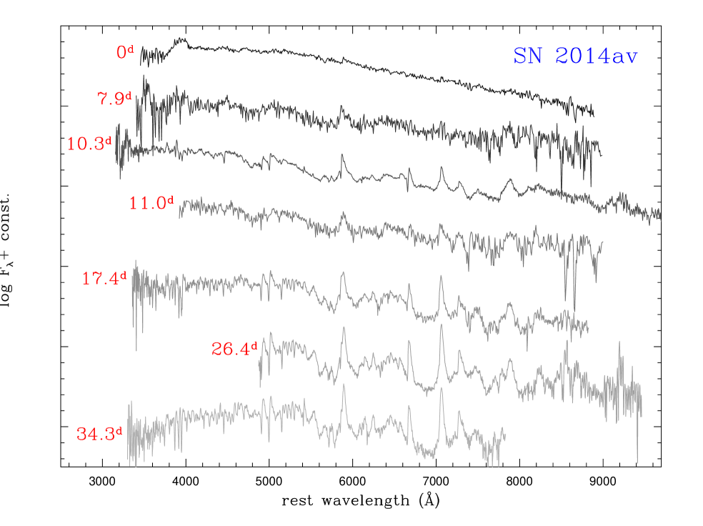
Figure 4: Spectral evolution of SN 2014av. The spectra have been Doppler-corrected, although no reddening correction has been applied.

SN 2014av was discovered soon after the explosion and a few days before maximum. Adopting the distance and reddening values reported in Section 1, SN 2014av reached an absolute magnitude of $-19.76\pm 0.16$ in the $R$ band, then it experienced a fast decline of $\sim$3 magnitudes. After about 25 days post-maximum, the light curve declined with a slower rate in all bands, as mentioned in Section 2 (see Table 4). A flattening of the optical light curve is unusual, but not unique in late Type Ibn SNe, viz. in OGLE-2012-SN-006 (Pastorello et al., 2015c). In order to better determine the photometric properties of SN 2014av in the context of SNe Ibn, we measured the main parameters of the $R$-band light curves for a wide sample of objects. In particular, we estimated (when possible) the absolute peak magnitudes, the duration of the rise phase to maximum, and the post-peak declines at three temporal windows: between maximum and +25 days ($\gamma^{R}_{0-25}$), from +25 days and +2 months ($\gamma^{R}_{25-60}$), and at later phases ($\gamma^{R}_{60-150}$). The results are reported in Table 5. When $R$-band observations were incomplete to estimate the above parameters, we included measures obtained in other bands, as specified in the footnote. From a rapid inspection of the table, we note that SNe Ibn are quite luminous, most of them having absolute $R$-band magnitudes close to $-$19, or exceeding that value. Only one object, the transitional Type Ibn/IIn SN 2005la (Pastorello et al., 2008b), appears to be significantly fainter than other SNe Ibn, although for other objects we have incomplete information to derive firm conclusions on their peak luminosity. However, despite most SNe Ibn are very luminous at maximum, the light curve shapes are widely heterogeneous.

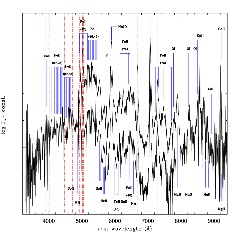
Figure 5: Identification of the most prominent lines in the late-time TNG spectra of SN 2014av. Dot-dashed vertical lines mark the rest wavelength positions of the strongest He I features.

This can be best highlighted in Figure 3, where the absolute $R$-band light curve of SN 2014av is compared with those of a wide sample of SNe Ibn. We also show unpublished data of the recent SN Ibn 2014bk (Morokuma et al., 2014), which is a relatively fast-evolving SN Ibn. Photometric data for this object are listed in Appendix A. The comparison shows that the light curves are significantly different among the objects of this family. The absolute magnitudes at peak of these SNe mainly range from -18 (iPTF13beo, Gorbikov et al., 2014) to -20 (SN 1999cq, Matheson et al., 2000). Some objects (e.g. SN 2010al and OGLE-2012-SN-006) show a slow rise to maximum (up to 16 days), but other SNe Ibn experience a very fast rise to the peak ($\leq$6 days). SN 2014av has an intermediate rise time of about 10 days. The post-peak decline is even more heterogeneous, with one object having a very fast-declining light curve after maximum (LSQ13ccw, Pastorello et al., 2015a), many with almost linear post-peak optical drops , and a few others showing double-phase light curve declines. The latter objects experience an initially fast decline, which is followed by a clear flattening at later stages. SN 2014av belong to this group, although the most extreme case is OGLE-2012-SN-006 (Pastorello et al., 2015c), with an early decline of about 5 mag/100^d, followed by a very long phase with a very flat light curve (0.4 mag/100^d from 25 and 60 days, and 1 mag/100^d later on). As a comparison, the $R$-band decline rate of SN 2010al at phases $>$ 1 month after maximum is about 3 mag/100^d, which is a factor 3 higher than the decline rate expected in a ⁵⁶Co-powered event. Finally, three objects (SN 2005la, SN 2011hw and iPTF13beo) showed a non-linear light curve decline after the first maximum, with at least one secondary luminosity peak (Pastorello et al., 2008b; Smith et al., 2012; Gorbikov et al., 2014; Pastorello et al., 2015b).

3 Spectroscopic Observations

The spectroscopic monitoring campaign of SN 2014av started $\sim$4 days after the SN discovery, and continued for about one month. Spectra have been collected using the Lijiang 2.4m telescope of the Yunnan Astronomical Observatory (YNAO) of the Chinese Academy of Sciences (equipped with YFOSC), the 3.58-m TNG with Dolores and the 2.56-m NOT with ALFOSC. Information on the spectroscopic observations is given in Table 6, the sequence of spectra available for SN 2014av is shown in Figure 4.

The earliest spectrum, obtained at maximum light (i.e. 10.6 days after the explosion), has poor S/N and modest resolution (see Table 6). It is characterised by a blue continuum, with superposed narrow and weak lines of He I, the most prominent being the $\lambda$5876 transition. Such line has a P-Cygni profile, whose minimum is blue-shifted by about $2100\pm 800$ km s^-1. A relatively strong feature detected at about 4700 Å (rest frame) is tentatively identified as He II $\lambda$4686. Another very prominent feature is detected at about 3950 Å, and is tentatively identified as a blend of He I and Ca II $\lambda\lambda$3934, 3968 (Ca II H$\&$K).

Subsequent spectra (at phases 7.9 day to 11 day after maximum) show a remarkable evolution. A blue pseudo-continuum typical of Type Ibn SNe and other interacting events is now visible. He I lines with low-contrast P-Cygni profiles are clearly detected: $\lambda$3889, $\lambda$4026, $\lambda$4472, $\lambda$4713, $\lambda$4922, $\lambda$5016 and $\lambda$5048. The He II $\lambda$4686 feature has now disappeared. Broader absorptions are attributed to blends of Fe II (see also Figure 5).

At redder wavelengths, very prominent He I lines are detected, with the emission component which dominates over the P-Cygni absorption: $\lambda$5876 (possibly blended with the Na I doublet), $\lambda$6678, $\lambda$7065 and $\lambda$7281. The position of the deep minimum of the He I $\lambda$6678 feature indicates a velocity of the He-rich wind of $940\pm 110$ km s^-1. However, the most prominent He I lines show a clear double-component profile. From deblending the $\lambda$7065 line with 2 Gaussian components, we infer a broader component with full width at half maximum (FWHM) velocity v${}_{FWHM}\approx$ 4500 km s^-1 (marginally evolving with time), with superimposed a narrow line with v${}_{FWHM}\approx 1000$ km s^-1 (not resolved in the YFOSC spectra). Numerous additional bumps and individual lines are detected between 5500 and 7000 Å, mostly due to Fe II lines. From these spectra there is marginal evidence for the presence of a weak H$\alpha$.

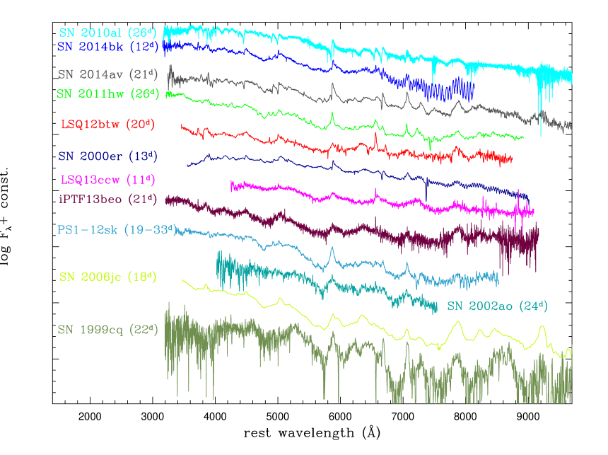
Figure 6: Collection of spectra of Type Ibn SNe obtained at phases between 11 and 26 days: SNe 2014av and 2014bk (this paper), SNe 2010al and 2011hw (Pastorello et al., 2015b), LSQ12btw and LSQ13ccw (Pastorello et al., 2015a), SNe 2000er ans 2002ao (Pastorello et al., 2008a), iPTF13beo (Gorbikov et al., 2014), PS1-12sk (Sanders et al., 2013), SN 2006jc (Pastorello et al., 2007) and SN 1999cq (Matheson et al., 2000). Phases reported in brackets are days from the presumed explosion epochs.

At the reddest edge of the optical spectral domain, we notice a broad emission at about 7890 Å, with v${}_{FWHM}\approx$ 4700 km s^-1. This is likely due to Mg II $\lambda$7877 and $\lambda$7896. Another shallow bump peaks at about 8200 Å, which we identify as Mg II $\lambda$8214 and $\lambda$8235. The wide red tail of this feature is possibly due to other Mg II lines ($\lambda$8735, $\lambda$8746, $\lambda$8824 and $\lambda$8835), although we cannot rule out a contribution from Ca II $\lambda\lambda\lambda$8498, 8542, 8662 (hereafter the NIR Ca II triplet). A further feature at about 9200 Å can be due to Mg II $\lambda$9218 and Mg II $\lambda$9244.

At later epochs, the emissions become stronger, and allow us to perform a more robust line identification. Using our latest TNG spectra (phases 26.4 days and 34.3 days after maximum) we accurately identify the most prominent spectral features in Figure 5. We still see the prominent He I lines, whose broad and narrow components have now v${}_{FWHM}\approx$ 2800 km s^-1 and v${}_{FWHM}\approx$ 1200-1300 km s^-1, respectively. Now Ca II H$\&$K and the NIR triplet are clearly discernible, with velocity of 1580 $\pm$ 230 km s^-1 (as measured from the positions of the minimum of the two Ca II H$\&$K lines). Mg II lines are still quite prominent, but at these phases, also O I features are identified: $\lambda\lambda\lambda$7772,7774,7775, $\lambda$8222, $\lambda$8446 (partially blended with Ca II NIR). Fe II lines with P-Cygni profiles are still detected, with average velocities of 1230 $\pm$ 120 km s^-1. From these later-epoch spectra, we also note the presence of Sc II lines. Again, we tentatively identify a weak H$\alpha$ emission, though alternative identifications cannot be ruled out (see also Section 5.2). In particular, assuming that it is H$\alpha$, its FWHM would be 820 km s^-1, which is consistent with the velocity inferred for the Fe II lines, although marginally slower.

3.1 Comparison with other Type Ibn SNe

The spectra of Type Ibn SNe are characterised by the presence of prominent and relatively narrow He I features. The heterogeneity of the photometric properties of SNe Ibn has been remarked in Section 2.1. In Figure 6, we compare a collection of spectra of SNe Ibn whose phases are approximately known, including an unpublished spectrum of SN 2014bk. The comparison in the figure highlights the existence of some heterogeneity among SNe Ibn also in their spectral observables. First of all, the velocities of the most prominent line components range from about 700 km s^-1 to a few thousands km s^-1 (and these velocities may be significantly phase-dependent). The wide velocity range probably depends on the gas regions where these lines originate, e.g. in the unperturbed CSM, in a shocked shell, in the shocked or unshocked SN ejecta or a combination of different emitting regions. We will further discuss the nature of the different components of the He I lines in Section 5.1. In addition, there are clear differences in the strengths of the broad $\alpha$-element lines, which are occasionally prominent (e.g. in SN 2006jc, Pastorello et al., 2007; Foley et al., 2007), and sometimes almost undetectable, like in the case of the Type Ibn/IIn SN 2005la (Pastorello et al., 2008b; Modjaz et al., 2014, see Section 5.3). In a few cases, narrow coronal lines were also detected in SNe Ibn (for example in SN 2011hw, Smith et al., 2012; Pastorello et al., 2015b). Finally, there is heterogeneity in the spectroscopic evolution time scales among the objects of the sample, which probably depends on the geometry and the distribution of the CSM with which the SN ejecta are interacting.

4 Quasi-bolometric light curve and physical parameters

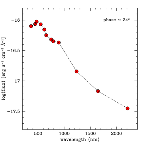
Figure 7: SED of SN 2014av computed on May 16, 2014, i.e. about 34 days after the explosion.

In order to constrain some basic physical parameters for SN 2014av, we computed its pseudo-bolometric light curve by integrating the flux contribution of individual optical bands. For each band, we derived the flux at the effective wavelength, considering only epochs with Sloan $r$-band observations being available. When individual photometric points at given epochs were not available, their contribution was computed using the magnitude information in adjacent epochs. Since early-time photometry (during the rising branch and around the light curve peak) was not available in most photometric bands, the early flux contribution in the missing bands was obtained assuming an early colour evolution of SN 2014av similar to that of the Type Ibn SN 2010al (Pastorello et al., 2015b).

The fluxes provided the spectral energy distribution (SED) at the given phase. The observed fluxes were integrated with the trapezoidal rule and converted to luminosity adopting the distance and interstellar reddening estimated in Section 1. We did not account for the UV flux contribution, although it might have been significant at early phases (see, e.g., Pastorello et al., 2015b), while we did estimate the NIR flux using the single 2014 May 16 NIR observation, under the very rough assumption of constant NIR contribution. The SED computed on May 16 is shown in Figure 7. The pseudo-bolometric light curve of SN 2014av is shown in Figure 8 (with and without the NIR contribution), and is compared with the light curves of the Type Ibn SNe 2006jc (data are from Pastorello et al., 2007, 2008a; Foley et al., 2007; Di Carlo et al., 2008), 2010al (Pastorello et al., 2015b) and OGLE-2012-SN-006 (Pastorello et al., 2015c). The most significant detection limits are also shown.

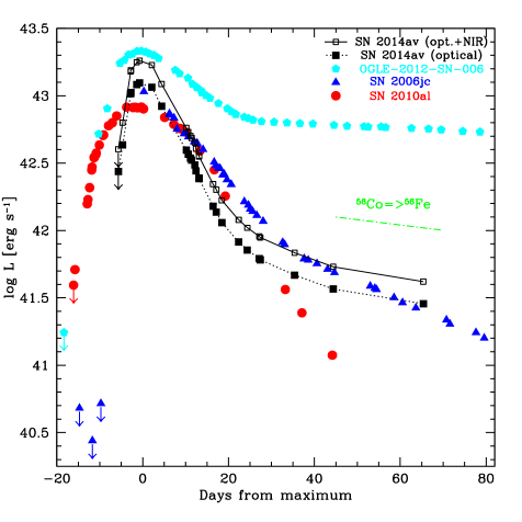
Figure 8: Pseudo-bolometric light curve of SN 2014av, with (solid line) and without (dotted line) the additional NIR contribution, as specified in the text. For comparison, also the bolometric light curves of the Type Ibn SNe 2006jc, 2010al and OGLE-2012-SN-006 are shown. For the comparison objects, the light curves are computed by integrating the contributions from the $U$ to the $K$ bands.

We confirm the large scatter in the photometric properties of SNe Ibn, as discussed in Sect. 2.1. Although SN 2014av (accounting from the NIR contribution) has a peak magnitude comparable with that of the very luminous OGLE-2012-SN-006, and is slightly more luminous at maximum than SNe 2006jc and 2010al, its photometric evolution is very fast. It experiences a very rapid rise to the light curve peak similar to that inferred for SN 2006jc, and has a post-peak decline which is faster than any other SN in the sample. However, it clearly flattens at phases above 20-25 days, to a luminosity similar to that of SN 2006jc, but with a slope which is twice as fast as the ⁵⁶Co to ⁵⁶Fe decay rate.

Assuming a modest contribution of the ejecta-CSM interaction to the observed luminosity evolution in SN 2014av, its high peak luminosity ($\sim 1.8\times 10^{43}$ erg s^-1) and its late-time light curve evolution would be indicative of a moderate ejected ⁵⁶Ni mass. As there is a decent match with the light curve of SN 2006jc, we would obtain for SN 2014av an amount of ⁵⁶Ni similar to the value inferred for SN 2006jc (0.2-0.3 M_⊙, Pastorello et al., 2008a; Tominaga et al., 2008). This value for the ⁵⁶Ni mass is relatively high for a core-collapse SN, although it has already been observed in some stripped-envelope SNe which ejected several solar masses of material (e.g. the “hypernovae”, Nomoto et al., 2006; Mazzali et al., 2013). On the other hand, it is very unlikely that SN 2014av ejected a few solar masses of material. In fact, it is well known that the evolutionary time-scale of the light curve in a non-interacting SN depends on the ejected mass to kinetic energy ratio (e.g. Arnett, 1982). As a consequence, a narrow (i.e. fast-evolving) light curve peak would probably be indicative of modest ejected masses, with a significant fraction of this material being composed by radioactive isotopes.

We note, however, that large M(⁵⁶Ni) / M_ej ratios are typical of thermonuclear explosion rather than canonical core-collapse events, and a thermonuclear explosion scenario is contradicted by other observables, including the preferential location of SNe Ibn in star-forming galaxies (e.g., Pastorello et al., 2015c), the strengths of $\alpha$-element spectral features and the detection of a pre-SN eruption in SN 2006jc, which is supportive of a massive progenitor. For all this, Type Ibn SNe are most likely core-collapse events. However, since the energy released in the radioactive decays alone cannot comfortably explain their observed evolution, alternative/additional powering mechanisms (including CSM-ejecta interaction) may provide more plausible explanations for the properties of SN 2014av and other Type Ibn SNe, as proposed by Chugai (2009).

5 Spectral characterization of Type Ibn supernovae

5.1 He I line velocity evolution

As discussed above and in other recent papers in the literature, SNe Ibn display a very wide range of observed properties. This is not in contrast with expectations, as wide heterogeneity in the observable is also observed - for example - in Type IIn SNe. The physical parameters of SNe Ibn strongly depend on the geometry, the composition, and the density profile of the CSM, along with the mass and the composition of the residual stellar envelope at the time of the terminal SN explosion.

A method to constrain the properties of the stellar wind and the nature of the line emitting regions is studying the evolution of the velocity of the spectral lines. Spectra of SNe interacting with a CSM (such as Type IIn and Type Ibn events) show lines with multiple-width components. These are though to be produced in different gas regions (Chevalier & Fransson, 1985, 1994; Chugai & Danziger, 1994; Chugai, 1997). Multiple components in the spectral lines, in fact, indicate that the emitting materials move at different velocities. Narrow lines (with velocities from a few hundreds to $\leq$ 2000 km s^-1) likely generate in slowly expanding, photo-ionized material. Very likely, this gas is unshocked CSM produced by the progenitor star before exploding as a SN. More controversial is the location of intermediate to broad components (from a few thousands to $\sim$ 10⁴ km s^-1): they can either be produced in a gas interface between two shock fronts (forward and reverse shocks), or in the freely expanding SN ejecta.

In SNe Ibn, hence, the study of the line profiles provides insights on the the velocity of the emitting material, and gives key information on the mass-loss history of the SN progenitors. When a clear P-Cygni profile is identified, the velocity of the He-rich expanding material is obtained by measuring the position of the core of the blue-shifted absorption. When this component is not detected, the velocity is estimated through the FWHM of the strongest He I emission lines, obtained after deblending the full line profile with Gaussian fits.

The evolution of the narrow components of the He I lines for the entire SN sample is shown in Figure 9, that of the intermediate-width components is shown in Figure 10. As velocities are measured from spectra available in the literature, in some cases only modest S/N spectra are available. This explains the large error bars occasionally shown in the figures. The velocities of the narrow He I component in SN 2011hw spectra are measured from the spectra published in Pastorello et al. (2015b), with the exception of two points in Figure 9, where we report measures performed by Smith et al. (2012) on moderate resolution spectra. For SN 2006jc, the spectra are taken from Pastorello et al. (2007, 2008a) and Anupama et al. (2009). A summary with the main outcomes from our inspection of the above SN spectra is reported in Table 7.

Table 7: Main properties of the spectra for the Type Ibn SN sample. In column 3, we report the velocities of the narrow He I line components, in column 4 the range of velocities measured for the intermediate/broad He I components, while in column 5 we comment the robustness of the H$\alpha$ line detection associated with the SN.

SN	Type	vnarrow(HeI) (km s-1)	vbroad(HeI) (range; km s-1)	H$\alpha$ detection	source
SN 1999cq	Ibn	1900	6150	no	1
SN 2000er	Ibn	1000	3950-4300	no	2
SN 2002ao	Ibn	940	3500-6050	weak	2
SN 2005la	Ibn/IIn	500	2000-4200	strong	3,a
SN 2006jc	Ibn	760	1700-3100	weak	3,4,5
SN 2010al	Ibn	1000-1250	2550-5800	weak	8
SN 2011hw	Ibn/IIn	210-250	1350-2350	moderate	8
PS1-12sk	Ibn	130	3100-3300	weak	9
OGLE-006	Ibn	800-1000	2400-3250	weak	10
LSQ12btw	Ibn	970	3200-5250	no	11
iPTF13beo	Ibn-pec	2070	4970	no	12
LSQ13ccw	Ibn-pec	2300	6750	uncertain	11
CSS140421	Ibn	unknown	unknown	unknown	13
ASASSN-14dd	Ibn	unknown	unknown	unknown	14
SN 2014av	Ibn	840-1240	4350-5000	weak	15
SN 2014bk	Ibn	1100	5950	uncertain	15
ASASSN-15ed	Ibn/Ib	1200-1500	6000-7000	no	16
PSN J07285387+3349106	Ibn	1000-1400	3000-3450	no	17
SN2015G	Ibn/Ib	$\sim$1300	$\sim$5500	no	18,19

1 = Matheson et al. (2000); 2 = Pastorello et al. (2008a); 3 = Pastorello et al. (2008b); a = Modjaz et al. (2014); 4 = Pastorello et al. (2007); 5 = Anupama et al. (2009); 8 = Pastorello et al. (2015b); 9 = Sanders et al. (2013); 10 = Pastorello et al. (2015c); 11 = Pastorello et al. (2015a); 12 = Gorbikov et al. (2014); 13 = Polshaw et al. (2014); 14 = Prieto et al. (2014); 15 = this paper; 16 = Pastorello et al. (2015d); 17 = Pastorello et al. (2015e); 18 = Ayani (2015); 19 = Foley et al. (2015).

5.1.1 Narrow He I line components

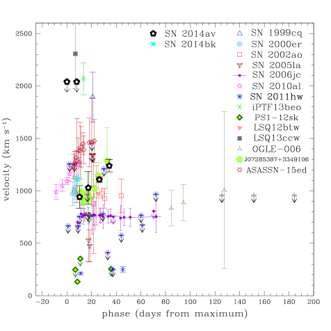
Figure 9: Evolution of the velocity of the narrow He I line components for our SN sample. The reported velocities are computed as the weighted average of the values inferred for the individual He I lines. The errors are computed as the standard deviation of individual He I line velocities. In early spectra of Type Ibn SNe, the velocities for the narrow He I lines were preferentially estimated from the position of the absorption minimum. At later epochs, when narrow absorptions were no longer visible, we estimated their velocities from the FWHM of the emission component.

The width of the narrow line components provides key information on the velocity of the unshocked He-rich CSM, and hence allows us to directly probe the pre-SN stellar wind. The temporal evolution of the velocity of the narrow He I line components is shown in Figure 9. When narrow components are not resolved in the spectra, we report in the figure only the resolution limits. First of all, for most objects we note a very modest, if any, evolution with time. This is what we expect from an unshocked circumstellar emitting shell.

The most remarkable finding from Figure 9 (see also Table 7) is that the narrowest components observed in the spectra of our Type Ibn SN sample span a wide range of velocities. Objects showing low velocities for the unperturbed CSM are the two transitional type Ibn, viz. SNe 2011hw (200-250 km s^-1) and 2005la (about 500 s^-1). In these two cases, an H$\alpha$ line associated with the SN is also detected, with moderate strength. The identification of H lines along with modest stellar wind velocities (a few hundreds km s^-1) are compatible with a star which is transitioning between the LBV and the Wolf-Rayet (WNE-type) stages, as proposed by Smith et al. (2012), Pastorello et al. (2008b) and Pastorello et al. (2015b). Another object showing remarkably small velocities for the narrow CSM He I lines is PS1-12sk, from which a relatively weak intermediate-component H$\alpha$ (with v${}_{FWHM}\sim$ 1600 km s^-1) is possibly detected in the post-peak spectra shown by Sanders et al. (2013) (see their figure 6).

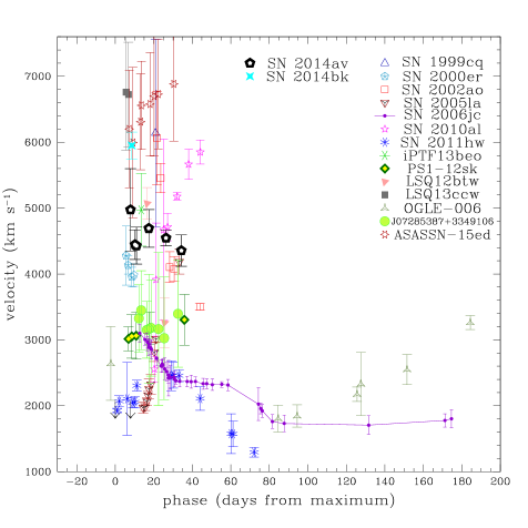
Figure 10: Like Figure 6, but for the intermediate He I line components. The reported velocities are computed as the weighted average among the measures available for the strongest He I lines. When a relatively broad P-Cygni absorption was clearly detected for the He I lines, the velocity was estimated from the position of the minimum. When the broad absorption was not detected, the velocity was measured as the FWHM velocity of the intermediate/broad emission components obtained after deblending the He I line profile. Although we are aware that these non-homogeneous criteria adopted in measuring line velocities may undermine the robustness of the outcomes, this is the best we can do with the available data. With this approach, we may offer for each SN an indicative estimate for the velocity of the fastest-moving detectable gas.

In most cases (including SN 2014av), the narrow He I components for our spectral sample have velocities around 800-1000 s^-1, while in three cases they widely exceed that value. In fact, SN 1999cq, iPTF13beo and LSQ13ccw show narrow components with P-Cygni profiles with v${}_{FWHM}\sim$ 1900-2300 km s^-1. It is worth noting that two of these three objects have unusual properties, with iPTF13beo showing a double-peaked light curve (Gorbikov et al., 2014), whilst LSQ13ccw has an extremely fast evolving light curve and some unique spectral features (see discussion in Pastorello et al., 2015c) with some similarity with the peculiar Type Ib SN 2002bj (Poznanski et al., 2010). Type Ibn SNe, whose spectra show weak or no trace of H lines, and velocities inferred for the narrow He I lines near or above 1000 km s^-1, most likely should be linked to more evolved Wolf-Rayet progenitors.

5.1.2 Intermediate/broad He I line components

Figure 10 shows the evolution of the expansion velocities as measured for the intermediate/broad components of the He I lines in our SN sample. The range of velocities for these components is reported in Table 7. They have velocities which are a factor 4-6 higher than those measured for the narrow components.

In contrast with the narrow features, the broader components of the He I lines are found to evolve significantly with time. In fact, the evolution of these components depends on the velocity of the ejecta and the density of the interacting material. Their velocities may provide clues for the gas interface between two shock fronts, which also depends on the speed of the expanding SN ejecta.

In particular, it is interesting to inspect the evolution of the spectral lines of SN 2010al: at phases around the light curve peak, the velocity inferred from the mimimum of the He I lines is $\sim$ 1000 km s^-1 (Table 7), consistent with that expected for the unshocked CSM. Thereafter, He I lines become broader with time, increasing to $\sim$ 4700 km s^-1 at about 4 weeks after the light curve peak, and reaching 5800 km s^-1 at 1.5 months post-maximum. Broad He I features with P-Cygni profile have been detected in ASASSN-15ed, with velocities of 6000–7000 km s^-1 (as inferred from the position of the core of the P-Cygni absorptions). As the SN is a transitional event from Type Ib to Type Ibn, these broad features are likely indicative of the speed of the expanding SN ejecta (Pastorello et al., 2015d). An increasing velocity of the intermediate/broad He I components is observed in the Type Ibn/IIn SN 2005la, with the gas velocity rising from about 2000 km s^-1 soon after discovery to $\sim$4200 km s^-1 about 3 weeks later.

However, in some cases, the He I lines become narrower with time (e.g., in SN 2002ao the He I intermediate component decreases its width by a factor 2 in 3 weeks). This is also observed in SN 2014av, although its intermediate-velocity component has a more modest velocity evolution, spanning from 5000 to 4300 km s^-1 in about 4 weeks. A similar moderate evolution of the He I intermediate components towards lower velocity values has been observed in SN 2006jc (from 3100 to 1700 km s^-1 in about 4 months). All of this suggests a decline in the velocity of the shocked gas regions, which may result from an increased density profile of the CSM gas. More complex is the evolution of the intermediate-component velocity of SN 2011hw. It grows from 1900 to 2500 km s^-1 during the first month, but then it declines to about 1300 km s^-1 at 70 days from the discovery. Again, this peculiar evolution can be ascribed to a complex density profile of the shocked gas region.

5.2 Detection of H$\alpha$

The detection of H$\alpha$ (and, eventually, other Balmer lines) is crucial to accurately classify interacting transients. Other ingredients for the classification are the detection of He I lines, and the relative strengths between H and He I features. Although narrow He I emission lines are frequently detected in the spectra of Type IIn SNe, the relative strengths between H$\alpha$ and the most prominent optical He I lines (in particular $\lambda$5876 and $\lambda$7065) determines the classification of the transient as a Type IIn, a Type Ibn or even a transitional object between these two SN types.

Balmer H lines are clearly detected in the two transitional Type Ibn/IIn SNe 2005la and 2011hw (Pastorello et al., 2008b, 2015b; Smith et al., 2012). In the spectra of these objects, the strength of H$\alpha$ is comparable with those of the most prominent He I lines. The velocity evolution inferred for the H lines in SN 2005la is very similar to that of the He I lines. In the early spectra of SN 2005la published by Modjaz et al. (2014), H$\alpha$ showed a narrow, marginally resolved (v${}_{FWHM}\sim$ 400 km s^-1) component, superposed on a broader base with a P-Cygni profile. The velocities deduced for the broader component evolved significantly with time, from about 1400 km s^-1 in the spectra close to the explosion epoch, to about 4000 km s^-1 in the spectra obtained about 3 weeks later. The highest resolution spectrum of SN 2011hw (Pastorello et al., 2015b) showed an unresolved H$\alpha$ (v${}_{FWHM}<$ 250 km s^-1) atop of broader wings that followed the velocity evolution observed for the He I lines (shown in Figure 10): the velocity of the intermediate H$\alpha$ component had a non monotonic evolution in the range between 1350 and 2350 km s^-1.

However, other Type Ibn events show no prominent H SN lines or, in some cases, the identification of H$\alpha$ is controversial, with an alternative identification of the feature as C II being plausible. In particular, blends of H$\alpha$ with C II $\lambda$6580 cannot be ruled out in most SNe of our sample, including SN 2014av. In particular, the detection of multiple lines of C II in the spectra of PS1-12sk (Sanders et al., 2013) argued - at least in the case of that object - against the identification of H lines. When the discrimination between H$\alpha$ and C II $\lambda$6580 is problematic, the identification of H$\alpha$ is indicated as “uncertain” in Table 7.

5.3 Detection of $\alpha$-element features

The robust detection of lines from heavier elements, in particular $\alpha$-elements such as O I, Mg II, Ca II and occasionally even Si II, has been confirmed for a number of Type Ibn SNe. In most cases, features from these ions have been observed in emission, with FWHM velocities higher or similar to those of the intermediate-width components of the He I lines (in the range between 2000 and 6000 km s^-1, depending on the SN and its phase).

Relatively broad O I and Mg II lines are frequently detected as strong emission features in the spectra of SNe Ibn. In particular, in SNe 1999cq and 2006jc, O I and Mg II lines are very prominent and with velocities v${}_{FWHM}\approx$ 5000-9000 km s^-1 (see, e.g., Matheson et al., 2000; Pastorello et al., 2007). These lines are clearly detected also in SN 2014av, though they are narrower than in other SNe Ibn, and with Mg II lines being stronger than O I features. A high relative strength of Mg II vs. O I lines has also been observed in the reddened PSN J07285387+3349106 (Pastorello et al., 2015e). We note, however, that O I and Mg II lines are weak in other SNe Ibn, including SN 2011hw, PS1-12sk, LSQ13ccw and LSQ12btw. Finally, in a few cases (e.g. in SNe 2000er and 2005la), the non-detection of these lines is ascribed to the early phases of the available spectra.

Also, the detection of the Ca II NIR feature is likely phase dependent, since this triplet is normally observed in spectra obtained a few weeks after the explosion. For this reason, the Ca II NIR remains undetected (or is very weak) in several objects, including SN 2000er, iPTF13beo, LSQ12btw, LSQ13ccw and PS1-12sk.

Less ubiquitous is the identification of Si II in the spectra of Type Ibn SNe. While Si II lines are clearly detected in a few objects (e.g. SNe 1999cq, 2000er, 2006jc LSQ12btw, iPTF13beo), these are not detected in other SNe of this class, including PS1-12sk, LSQ13ccw, SN 2005la and OGLE-2012-SN-006.

6 About the environments and Type Ibn SN progenitors

Pastorello et al. (2015a) made a preliminary attempt to characterise the host galaxies of the sample of SNe Ibn considered in this paper. All SNe Ibn have been discovered in spiral galaxies, with the remarkable exception of PS1-12sk, which exploded in the outskirts of an elliptical galaxy (Sanders et al., 2013). Accounting for the great predominance of spiral galaxies among the hosts of SNe Ibn, it is natural to associate this SN type with massive stellar population.

SN 2014av exploded in a spiral (Sb-type) galaxy, the most luminous one ever observed hosting a SN Ibn ($M_{B}=-21.8$, Pastorello et al., 2015a). The oxygen abundance inferred at the SN position is about 9.2 (Pastorello et al., 2015a), suggesting a metal-rich environment. However, other metallicity estimates of Type Ibn SN environments led to different conclusions (see, e.g., Appendix B). Pastorello et al. (2015a) estimated an average metallicity at the SN position of $<$ 12 + log (O/H) $>$ = 8.63 $\pm$ 0.42 for the sample, which is not particularly sub-solar, although there is a wide range in the values inferred for individual SNe. Using a smaller sample, Taddia et al. (2015) inferred a slightly lower oxygen abundance, viz. $<$ 12 + log (O/H) $>$ = 8.45 $\pm$ 0.10. A large dispersion in the values of the oxygen abundance suggests that metallicity plays a marginal role in producing SNe Ibn.

The detection of a major outburst before the explosion of SN 2006jc (Pastorello et al., 2007; Foley et al., 2007) was one of the arguments used to support the association of the SN with an erupting massive Wolf-Rayet star. In other words, the precursor of SN 2006jc was very likely a Wolf-Rayet with a residual LBV-like behaviour. Although direct evidence of similar pre-SN eruptions is still missing in other Type Ibn SNe, the study of the properties of the He-rich CSM presented in this paper (including the constraints on the line velocities and the secure identification of $\alpha$-elements) supports massive progenitors for most SNe Ibn. However, the observed differences in their photometric and spectroscopic behaviour suggest some heterogeneity in the properties of the progenitor stars. In particular, the evidence of variable signatures of H in the CSM, the fact that the CSM velocities inferred from the narrow He I lines span one order of magnitude (from 200 to 2000 km s^-1, see Figure 9) and the variable amount of He still present in the stellar envelope at the moment of the SN explosion indicate that a wide range of sub-types of Wolf-Rayet stars, spanning from the transitional Opfe/WN9 stars to more stripped WC/O types (see Smith et al., 2012, and references therein), can very likely produce Type SNe Ibn SNe. In this context, observations of the transitional WN to WC-type Wolf-Rayet star NaSt1 (also known as Wolf-Rayet 122, Mauerhan et al., 2015) suggest that the binary interaction may favour the transition among Wolf-Rayet sub-types via pre-SN bursts, favouring the heterogeneity in the final Wolf-Rayet properties soon before their core-collapse. Finally, the similarity of - at least - SN Ibn LSQ13ccw with the peculiar SN Ib 2002bj (for which a helium detonation on a white dwarf scenario has been proposed by Poznanski et al., 2010) has been mentioned in Pastorello et al. (2015a).

7 Summary and final remarks

We have presented optical spectroscopic and photometric data of the recent, well-monitored Type Ibn SN 2014av. The object was discovered a few days before the light-curve maximum, and monitored for 2 months after the peak. Deep pre-explosion non-detection limits, along with a few photometric points obtained during the rising phase to the maximum light, allowed us to estimate the explosion epoch with a very small uncertainty to be JD = 2456760.5.

SN 2014av is one of the most luminous SNe Ibn in our sample, reaching an absolute magnitude $M_{R}=-19.78$ and a bolometric luminosity of about 1.8 $\times$ 10⁴³ erg s^-1. Despite the remarkable intrinsic luminosity, it is a relatively fast-evolving transient. In fact, although the rise time to maximum is not extremely short (10.6 days), the post-peak decline is very fast (see Tables 4 and 6). The spectra of SN 2014av evolve from showing an almost featureless continuum at early phases, to being dominated by intermediate-velocity He I lines, with relatively broad features from $\alpha$-elements. These later spectra are characterized by the unusual presence of a multiplicity of Fe II lines showing P-Cygni profiles.

SN 2014av has been compared with other objects classified as Type Ibn events, and - not unexpectedly - we have observed that a large heterogeneity exists among the objects of this class (in analogy with that observed in Type IIn SNe). In particular,

• although most SNe Ibn are luminous ($M_{R}<<-18$), there are rare exceptions of significantly weaker events (such as SN 2005la);

• differences are observed in the photometric evolutionary time-scales, with objects showing extremely fast-evolving light curves (such as that of LSQ13ccw; Pastorello et al., 2015a) and others with very slow-evolving light curves resembling those of SNe IIn (e.g., OGLE-2012-SN-006; Pastorello et al., 2015c);

• light curves of SNe Ibn may show non-monotonic post-peak declines (see, e.g., the double-peaked light curve of iPTF13beo; Gorbikov et al., 2014);

• a range of FWHM velocities is observed for the narrow He I line components of SNe Ibn, indicating intrinsic differences in the progenitor wind velocities;

• relatively broad He I components can be detected in Type Ibn SN spectra, suggesting the presence of residual He in the envelope of their progenitor stars;

• in a few cases, SNe Ibn spectra have circumstellar Balmer lines, suggesting the presence of a small and variable fraction of H in the composition of their CSM (Smith et al., 2008; Pastorello et al., 2008b, 2015b).

The heterogeneous observed parameters of Type Ibn SNe likely depend on the different pre-explosion configuration and chemical composition of their progenitor systems.

The host of SN 2014av is a luminous ($M_{B}=-21.8$) Sb-type galaxy. In most cases, the galaxies hosting SNe Ibn are spirals, hence environments with active star formation, with the remarkable exception of PS1-12sk (Sanders et al., 2013) that exploded in the outskirts of an elliptical galaxy. For this reason, we favour the association of SN 2014av and other Type Ibn SNe with a massive stellar population. Thus, Wolf-Rayet stars of different sub-types are natural candidates to be the precursors of Type Ibn SNe. As discussed in Pastorello et al. (2015a), the oxygen abundance at the SN position is super-solar, being about 9.2, the highest in the Type Ibn SN sample. Since most Type Ibn SNe had exploded in environments showing a broad metallicity range (7.8 $<$ 12+log(O/H) $<$ 9.2), metallicity has very likely a marginal role in producing SNe Ibn.

Appendix A Optical photometry of SN 2014bk

In Table 8, we report sparse photometry available for the Type Ibn SN 2014bk, included in the SN sample discussed in this paper. These data have been reduced following standard prescriptions, as described in Section 2.

Table 8: Optical Johnson-Cousins magnitudes of SN 2014bk, and associated errors.

Obs. date	Average $JD$	$U$	$B$	$V$	$R$	$I$	Instrument
2014/06/05	2456813.55	–	–	–	17.976 (0.236)	–	1
2014/06/08	2456816.54	18.021 (0.076)	18.782 (0.054)	18.635 (0.047)	18.631 (0.077)	18.274 (0.071)	1
2014/06/20	2456829.43	19.591 (0.087)	20.096 (0.130)	19.729 (0.075)	19.898 (0.203)	19.685 (0.234)	1
2014/07/02	2456840.55	21.240 (0.185)	21.485 (0.144)	21.226 (0.126)	21.649 (0.282)	20.381 (0.268)	1
2014/08/15	2456885.37	–	–	–	$>$22.22	–	2

1 = 2.56-m NOT + ALFOSC (La Palma, Canary Islands, Spain); 2 = 10.4-m GTC + OSIRIS (Sloan $r$-band observation transformed into Johnson-Cousins data; La Palma, Canary Islands, Spain).

Appendix B Spectrum of the galaxy hosting SN 2014bk

A late-time spectrum of the comparison Type Ibn SN 2014bk was obtained at the 10.4-m Gran Telescopio Canarias (GTC) of the Observatorio del Roque de los Muchachos in La Palma (Canary Islands). The spectrum (shown in Figure 11) was obtained on 2014 August 15 (JD = 2456885.39) using OSIRIS and the R300B grism (resolution 17 Å); it shows no signature of the SN, but is useful to constrain the oxygen abundance at the SN location. The host galaxy, SDSS J135402.41+200024.0, has an estimated redshift z = 0.0697 (Morokuma et al., 2014).

In the spectrum, we securely identified several emission lines, the strongest being [O II] $\lambda$3927, [O III] $\lambda$5007 and H$\alpha$. Line fluxes for the strongest lines are reported in Table 9. In order to estimate the oxygen abundance, we measured the fluxes of a few relevant lines (including H$\alpha$, H$\beta$ [O III] $\lambda$5007 and [N II] $\lambda$6584), and applied the N2 and O3N2 methods desctibed in Pettini & Pagel (2004). The two indicators provide very consistent estimates, resulting in an average aboundance $<$ 12 + log (O/H) $>$ = 8.11 dex, which is largely sub-solar.

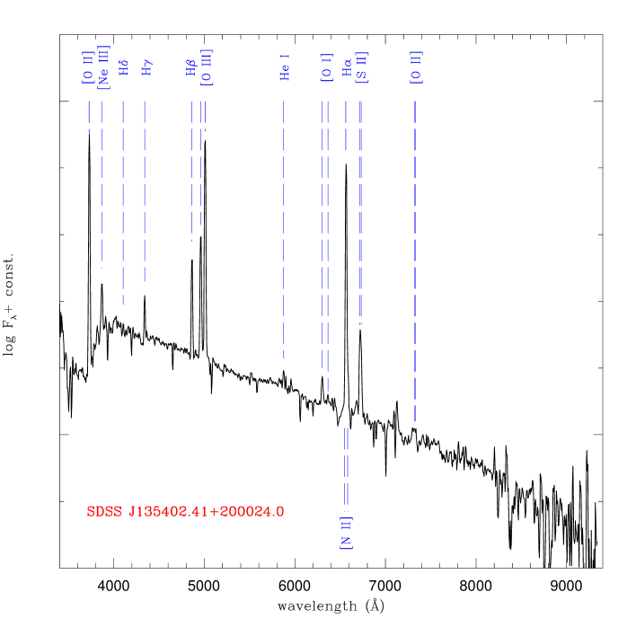
Figure 11: GTC (Osiris) spectrum of the galaxy hosting SN 2014bk, centered at the location of the SN.

Table 9: Observed fluxes for the strongest emission lines in the GTC + Osiris spectrum of SDSS J135402.41+200024.0.

Line	$\lambda$ (Å)	Flux (10-16 erg s-1 cm-1)
$[$O II$]$	3727	18.56 $\pm$ 0.54
$[$Ne III$]$	3868	2.41 $\pm$ 0.34
H$\gamma$	4340	1.70 $\pm$ 0.23
H$\beta$	4861	5.01 $\pm$ 0.26
$[$O III$]$	4959	6.55 $\pm$ 0.42
$[$O III$]$	5007	17. 89 $\pm$ 0.57
H$\alpha$	6563	16.37 $\pm$ 0.90
$[$N II$]$	6584	0.69 $\pm$ 0.32
$[$S II$]$	6717,6731	4.26 $\pm$ 0.31
$[$O II$]$	8320,8330	0.78 $\pm$ 0.25

References

- Anupama et al. (2009) Anupama, G. C., Sahu, D. K., Gurugubelli, U. K., Prabhu, T. P., Tominaga, N., Tanaka, M., Nomoto, K. 2009, MNRAS, 392, 894
- Arnett (1982) Arnett, W. D. 1982, ApJ, 253, 785
- Ayani (2015) Ayani, K. 2015, CBET, 4087, 2
- Bianco et al. (2014) Bianco, F. B., et al. 2014, ApJS, 213, 19
- Cappellaro (2014) Cappellaro, E. 2014. “SNOoPy: a package for SN photometry”; http://sngroup.oapd.inaf.it/snoopy.html
- Chassagne (2000) Chassagne, R. 2000, IAU Circ. 7528, 1
- Chevalier & Fransson (1985) Chevalier R. A., Fransson C. 1985, in ‘Supernova interaction with circumstellar wind and the distance to SN 1979C’ in N. Bartel ed., Supernovae as distance indicators, Springer: Berlin, p. 123
- Chevalier & Fransson (1994) Chevalier, R. A., Fransson, C. 1994, ApJ, 420, 268
- Chugai & Danziger (1994) Chugai N. N., Danziger J. J. 1994, MNRAS, 268, 173
- Chugai (1997) Chugai, N. N. 1997, Ap&SS, 252, 225
- Chugai et al. (2004) Chugai et al. 2004, MNRAS, 352, 1213
- Chugai (2009) Chugai, N. N. 2009, MNRAS, 400, 866
- Corsi et al. (2014) Corsi, A. et al. 2014, ApJ, 782, 42
- Di Carlo et al. (2008) Di Carlo, E. et al. 2008, ApJ, 684, 471
- Dilday et al. (2012) Dilday, B. et al. 2012, Science, 337, 97
- Fassia et al. (2001) Fassia, A. et al. 2001, MNRAS, 325, 907
- Foley et al. (2007) Foley, R. J., Smith, N., Ganeshalingam, M., Li, W., Chornock, R., Filippenko, A. V. 2007, ApJ, 657, L105
- Foley et al. (2015) Foley, R. J., Zheng, W., Filippenko, A. V., Van Dyk, S. D. 2015, Astron. Tel. 7298
- Fransson et al. (2002) Fransson, C. et al. 2002, ApJ, 572, 350
- Gorbikov et al. (2014) Gorbikov, E. et al. 2014, MNRAS, 443, 671
- Immler et al. (2008) Immler, S., et al. 2008, ApJ, 674, L85
- Kankare et al. (2012) Kankare, E. et al. 2012, MNRAS, 424, 855
- Landolt (1992) Landolt A. U. 1992, AJ, 104, 340
- Matheson et al. (2000) Matheson, T. et al. 2000, AJ, 119, 2303
- Mattila et al. (2008) Mattila, S. et al. 2008, MNRAS, 389, 141
- Mazzali et al. (2013) Mazzali, P. A., Walker, E. S., Pian, E., Tanaka, M., Corsi, A., Hattori, T., Gal-Yam, A. 2013, MNRAS, 432, 2463
- Mauerhan et al. (2015) Mauerhan, J. C. et al. 2015, MNRAS, 450, 2551
- Modjaz et al. (2014) Modjaz, M. et al. 2014, AJ, 147, 99
- Mould et al. (2000) Mould, J. R. et al. 2000, ApJ, 529, 786
- Morokuma et al. (2014) Morokuma, T. et al. 2014, CBET 3894
- Nomoto et al. (2006) Nomoto, K., Tominaga, N., Umeda, H., Kobayashi, C., Maeda, K. 2006, NuPhA, 777, 424
- Nozawa et al. (2008) Nozawa, T., et al. 2008, ApJ, 684, 1343
- Pastorello et al. (2002) Pastorello, A. et al. 2002, MNRAS, 333, 27
- Pastorello et al. (2007) Pastorello, A. et al. 2007, Nature, 447, 829
- Pastorello et al. (2008a) Pastorello, A. et al. 2008a, MNRAS, 289, 113
- Pastorello et al. (2008b) Pastorello, A. et al. 2008b, MNRAS, 289, 131
- Pastorello et al. (2015a) Pastorello, A. et al. 2015a, MNRAS, 449, 1954
- Pastorello et al. (2015b) Pastorello, A. et al. 2015b, MNRAS, 449, 1921
- Pastorello et al. (2015c) Pastorello, A. et al. 2015c, MNRAS, 449, 1941
- Pastorello et al. (2015d) Pastorello, A. et al. 2015d, MNRAS, 453, 3649
- Pastorello et al. (2015e) Pastorello, A. et al. 2015e, MNRAS, 454, 4293
- Paturel et al. (2003) Paturel, G., Petit, C., Prugniel, Ph., Theureau, G., Rousseau, J., Brouty, M., Dubois, P., Cambrésy, L. 2003, A&A, 412, 45
- Pettini & Pagel (2004) Pettini, M., Pagel, B. E. J. 2004, MNRAS, 348, L59
- Polshaw et al. (2014) Polshaw, J. et al. 2014, Astron. Tel. 6091
- Poznanski et al. (2010) Poznanski, D. et al. 2010, Science, 327, 58
- Prieto et al. (2014) Prieto, J. L. et al. 2014, Astron. Tel. 6293
- Sakon et al. (2009) Sakon, I., et al. 2009, ApJ, 692, 546
- Sanders et al. (2013) Sanders, N. E. et al. 2013, ApJ, 769, 39
- Schlafly & Finkbeiner (2011) Schlafly, E. F., Finkbeiner, D. P. 2011, ApJ, 737, 103
- Skrutskie et al. (2006) Skrutskie, M. F. et al. 2006, AJ, 131, 1163
- Smith et al. (2008) Smith, N., Foley, R. J., Filippenko, A. V. 2008, ApJ, 680, 568
- Smith et al. (2009) Smith, N. et al. 2009, ApJ, 695, 1334
- Smith et al. (2012) Smith, N. et al. 2012, MNRAS, 426, 1905
- Stanek et al. (2014) Stanek, K. Z. et al. 2014, Astron. Tel. 6269
- Stritzinger et al. (2012) Stritzinger et al. 2014, ApJ, 756, 173
- Taddia et al. (2015) Taddia, F. et al. 2015, A&A, 580, 131
- Tominaga et al. (2008) Tominaga, N. et al. 2008, ApJ, 687, 1208
- Trundle et al. (2009) Trundle, C. et al. 2009, A&A, 504, 945
- Turatto et al. (2003) Turatto, M., Benetti, S., Cappellaro, E. 2003, in Hillebrandt W., Leibundgut B., eds, Proc. ESO/MPA/MPE Workshop, From Twilight to Highlight: The Physics of Supernovae. Springer-Verlag, Berlin, p. 200
- Turatto & Pastorello (2014) Turatto, M., Pastorello, A. 2014, in Supernova Environmental Impacts, Proceedings of the International Astronomical Union, IAU Symposium, Volume 296, pp. 63-67
- Xu & Gao (2014) Xu, Z., & Gao, X. 2014, CBET, 3865, 1
- Yusa et al. (2015) Yusa, T., Shima, K., Buczynski, D., Noguchi, T., Nakano, S., Kiyota, S., Masi, G. 2015, CBET, 4087, 1
- Zhang et al. (2012) Zang, T. et al. 2012, AJ, 114, 131
- Zhang & Wang (2014) Zang, J.-J., & Wang X.-F., X. 2014, CBET, 3865, 2