Coarse Quantum Measurement : an analysis of the Stern-Gerlach Experiment

Abstract

We study the Quantum Measurement Process in a Stern-Gerlach setup with the spin of a silver atom as the quantum system and the position as the apparatus. The system and the apparatus are treated quantum-mechanically using unitary evolution. The new ingredient in our analysis is the idea that the probes determining the position of the silver atom are limited in resolution. We show using a Wigner matrix that due to the coarseness of the detection process, the pure density matrix appears to evolve to an impure one. We quantify the information gained about the spin in a coarse position measurement.

1 Introduction

Quantum mechanics is a very successful theory for describing the microscopic world of atoms. However, ever since its inception there are certain fundamental aspects of quantum theory that have remained obscure. This has to do with the relation between unitary evolution which is central to the theory, and the measurement process, which gives us information about the quantum system. The challenge that remains is a self consistent formulation of quantum theory which explains unitary evolution and outcomes of a measurement within a single framework.

Bohr had taken a semiclassical approach in which he viewed the apparatus classically and treated the system (spin) quantum mechanically. Such a point of view is unsatisfactory since at a fundamental level the world is governed by quantum mechanics. In this letter, we present a completely quantum mechanical analysis of the Stern-Gerlach experiment. Our purpose is to explore, in a simple solvable context, the idea that coarseness of the experimental probes is responsible for apparent non unitarity in the measurement process.

We focus on the Stern-Gerlach experiment as a context for understanding the measurement process in quantum mechanics without invoking any ad hoc assumption beyond pure unitary evolution. Let us begin by summarizing the Stern-Gerlach experiment. The set up consists of a beam of silver atoms (spin-${\frac{1}{2}}$ particles) moving along the $z$ direction passing through an inhomogeneous magnetic field along the $y$ direction. Two spots appear on the screen corresponding to the $y$ component of the spin, $S_{y}=\frac{1}{2}$ and $S_{y}=-\frac{1}{2}$. There have been a few analytical studies of this experiment in the past couple of decades[1, 2, 3, 4, 5, 6, 7, 8]. Some studies[7] invoke Ehrenfest’s Theorem to address the issue of measurement in a Stern-Gerlach setup. There have also been detailed analyses of the Stern-Gerlach experiment from the point of view of environment induced decoherence[1, 2, 6, 9]. In this letter we invoke the new idea that there is an inherent coarseness in the detection process. The role of coarseness of the measurement process in the quantum to classical transition has been explored in the past[10, 11, 12]. In [10, 11] coarseness of the measurement process has been investigated by using the Leggett-Garg inequality as a way of probing the quantum to classical transition. In [12] coarse graining has been used as a probe for detection of entanglement between a microscopic system and a macroscopic system. We present an analysis which offers a new perspective on the Stern-Gerlach experiment from the point of view of the coarseness of the measurement process.

The letter is organized as follows. We first summarize the measurement process. Then we present a theoretical analysis of the Stern-Gerlach experiment using unitary evolution. We show with a Wigner function matrix approach, that a coarse measurement with a finite spatial resolution leads to an apparently non unitary evolution for the Wigner matrix. Finally we end our letter with a concluding discussion.

2 The Measurement Process

Let us summarize the measurement process in quantum mechanics. Our system is initially in a coherent superposition of states $|S\rangle=\sum_{i}c_{i}|S_{i}\rangle$ in an orthonormal basis which diagonalises the quantity being measured. To begin with, the system plus apparatus is in the product state $|\psi\rangle=|S\rangle|A\rangle$, in which the system and apparatus are unentangled. It is useful to logically break up the measurement process into three steps. The first step in the measurement process entails coupling between the quantum system and the measuring apparatus so that the total state evolves unitarily to an entangled state $U|{\psi}\rangle=\sum_{i}c_{i}|S_{i}\rangle|A_{i}\rangle$. This state can be represented as a pure density matrix

$$\rho=|\psi\rangle\langle\psi|=\sum_{ij}c^{*}_{j}c_{i}|S_{i}\rangle|A_{i}\rangle\langle S_{j}|\langle A_{j}|$$ (1)

After the second step, the density matrix of the system takes the impure form

$$\tilde{\rho}=\sum_{i}|c_{i}|^{2}|S_{i}\rangle\langle S_{i}|$$ (2)

which is interpretable as a classical mixture of states. Finally, the impure diagonal density matrix (2) goes over to a pure state $c_{i}|S_{i}\rangle\langle S_{i}|c_{i}^{*}$. The first step can be explained entirely in terms of unitary evolution and therefore is not controversial. The final step, sometimes called “collapse”, has been debated extensively as the “quantum measurement problem”. This singling out of one outcome from many possibilities is not addressed here. Let us note that, even in classical probability theory, there is a singling out of one from several outcomes (only one horse wins the race). We address here the second step; the transition from quantum superpositions to classical mixtures. This is the focus of our letter. In this letter, we investigate the Stern-Gerlach experiment from the perspective of coarse quantum measurement (CQM), in which we recognize the fact that all experiments are constrained by bounded resources. We model these constraints by using a screen whose size and spatial resolution are fixed. The spatial resolution of the screen is given by the pixel size and the size of the screen determines the total number of pixels. Experimentally one can only say that an atom was incident on our screen somewhere within a pixel. Fixing these resources imposes ultraviolet as well as infrared cutoffs on the experimental probes. In this letter we are more concerned with the short distance cutoff.

3 Stern-Gerlach

Consider silver atoms with spin $\frac{1}{2}$ at rest in the laboratory, in a magnetic field given by

$$B=(B_{0}y,B_{0}x,0).$$

Notice that this field is both divergence and curl free. We confine the atoms to the $x$-$z$ plane and thus set $y=0$. The Hamiltonian for the system is

$$H=\frac{p^{2}}{2m}+Fx\sigma_{y}$$ (3)

where

$$F=-g\mu_{B}\frac{\hbar}{2}B_{0},$$

with $g$ the Landé $g$ factor and $\mu_{B}$ the Bohr magneton. The Schrödinger equation for the system is given by(See Appendix A)

$$i\hbar\frac{\partial{\psi}}{\partial t}=-\frac{\hbar^{2}}{2m}{\nabla^{2}\psi}+Fx\sigma_{y}\psi,$$ (4)

where $\psi$ is a two component Pauli spinor. This problem can be solved exactly by transforming from the laboratory frame to a freely falling frame $\xi=x-\frac{1}{2}at^{2}$ and $T=t$, with $a=F/m$ the acceleration and $\psi=e^{if}\phi$ (where, $f=\frac{maT}{\hbar}(\xi+\frac{1}{3}aT^{2})$), (which reduces it to a free particle problem as in the Einstein elevator) and then transforming back to the laboratory frame[13](See Appendix A). Such an analysis is entirely quantum mechanical. We view the spin as a quantum system and the position of the silver atom as the apparatus or pointer. We do not invoke any semiclassical approximation. The formulation above results in a separation in time of the two spin states. This can be mapped to the formulation(See Appendix A), of a typical experiment, where the separation of the spins happens in space and we will sometimes use the spatial notation and language with the understanding that $t=zm/k\hbar$, where $\hbar k=\sqrt{2mE}$. We start with an initial Gaussian wave packet of width $\sigma$. Setting $t=t_{f}-t_{i}$ our analysis gives the following exact propagators $K^{++}(x,x_{i};t)$, $K^{--}(x,x_{i};t)$ and $K^{+-}(x,x_{i};t)$[14, 15](See Appendix A), where the symbols $+$ and $-$ refer to the two components $\phi_{+}$ and $\phi_{-}$ of the Pauli spinor $\phi$.

$$K^{++}(x,x_{i};t) = \sqrt{\frac{m}{2\pi i\hbar t}}{\exp}i[m\frac{(x-x_{i})^{2}}{2\hbar{t}}$$ (5)

$$-\frac{Ft(x+x_{i})}{2\hbar}-\frac{F^{2}t^{3}}{24m\hbar}]$$

$$K^{--}(x,x_{i};t) = \sqrt{\frac{m}{2\pi i\hbar t}}{\exp}i[m\frac{(x-x_{i})^{2}}{2\hbar t}$$ (6)

$$+\frac{Ft(x+x_{i})}{2\hbar}-\frac{F^{2}t^{3}}{24m\hbar}]$$

$$K^{+-}(x,x_{i};t)=0$$ (7)

The final wave function is got by “folding” the initial Gaussian with the propagator matrix (Eqs.5-7). It has the form

$$\phi(x,t)=c_{+}\phi_{+}(x,t)|+\rangle+c_{-}\phi_{-}(x,t)|-\rangle,$$

where $|+\rangle$ and $|-\rangle$, are eigenstates of $\sigma_{y}$ and $\phi_{+}(x,t)$ and $\phi_{-}(x,t)$ are Gaussian wave packets (See Appendix A). We can identify two relevant time scales (Eqs. A-16 and A-17 of Appendix A): $\tau_{1}=\sqrt{\frac{2\sigma}{a}}$, the time over which the centers of mass of the two wave packets separate and $\tau_{2}=\frac{m\sigma^{2}}{\hbar}$, the timescale over which the individual wavepackets spread. We use the values $m=1.79\times 10^{-25}kg$, $F=9.27\times 10^{-22}N$ and $\sigma=10^{-6}m$ which are experimentally reasonable. Typical values for the two time scales are $\tau_{1}=10^{-5}s$ and $\tau_{2}=10^{-3}s$.

We restrict our discussion to a situation where the detection screen is placed at a location just at the point where the atom exits the magnetic field. However, in general one can have a further free evolution of the separated wavepackets beyond this region in the field free space (See Appendix).

The full density matrix (See Appendix B) is of the form:

$$\rho_{\alpha\beta}(x,x^{\prime})=c_{\alpha}\phi_{\alpha}(x)c_{\beta}^{*}{\phi}^{*}_{\beta}(x^{\prime}),$$ (8)

where $\alpha$ and $\beta$ take values $+$ and $-$. In Eq.(8) we have suppressed the time dependence in the notation.

4 Entanglement and Coarse Graining

The total density matrix of the system has entanglement between the spin and atomic position. The degree of entanglement can be measured by the entanglement entropy [16], which is most easily computed by tracing over the position and diagonalising the $2\times 2$ reduced density matrix $\rho_{spin}$ for the spin. The result is

$$S_{ent} = -Tr[\rho_{spin}\log\rho_{spin}]$$ (9)

$$= \log{2}-\frac{(1+A(t))}{2}\log{(1+A(t))}$$

$$-\frac{(1-A(t))}{2}\log{(1-A(t))}$$

where $A(t)=\exp{-\frac{t^{2}(t^{2}+\tau_{2}^{2})}{\tau_{1}^{4}}}$. Here and below, we set $c_{+}=c_{-}=1/\sqrt{2}$ for simplicity. The entanglement entropy is plotted in Fig. 1, which shows that $S_{ent}(t)$, starts from zero at $t=0$, then increases and finally settles down to an asymptotic value of $\log{2}$ over a time scale of the order of $10^{-7}s$. This entanglement timescale is given by $\tau_{3}=\tau_{1}{}^{2}/\tau_{2}$ and is shorter than the separation or spreading timescales. For $\tau_{1}\sim t>>\tau_{3}$, the entanglement is high even though the wavepackets have not cleanly separated in real space(Fig. 2).

From the density matrix $\rho_{\alpha\beta}(x,x^{\prime})$ we construct the Wigner matrix $\mathbf{W}(q,p)$ [9], using the standard variables $q=(x+x^{\prime})/2$ and $y=(x-x^{\prime})$. The matrix elements of $\mathbf{W}(q,p)$ are:

$$W_{\alpha\beta}(q,p)=\frac{1}{2\pi\hbar}\int_{-\infty}^{+\infty}{\rho_{\alpha\beta}(q+y/2,q-y/2)e^{\frac{ipy}{\hbar}}dy}$$ (10)

with $\alpha$, $\beta=\pm$. $\mathbf{W}(q,p)$ is a $2\times 2$ Hermitean matrix (not necessarily positive). All components of $\mathbf{W}(q,p)$ can in principle be measured by having a Stern-Gerlach setup at the screen to measure $Tr[\mathbf{W}(q,p)(1\!\!1+\hat{n}.\vec{\sigma})/2]$. In Figs $3$ and $4$, we display the function $W(q,p)={\rm Tr}[\mathbf{W}(q,p)(1\!\!1+\sigma_{x})/2]$, which shows the diagonal as well as off diagonal terms in the $|+\rangle,|-\rangle$ basis.

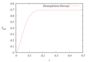
Figure 1: Figure shows the entanglement entropy as a function of time in units of $\mu s$.

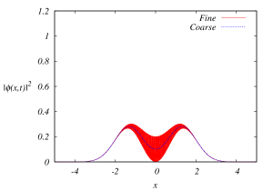
Figure 2: Figure shows the spatial distribution of the wavepacket at t=22.5$\mu$ sec. We have used the typical values $m=1.79\times 10^{-25}kg$, $F=9.27\times 10^{-22}N$, $\sigma=10^{-6}m$.

We now use the fact that the detection is done coarsely: the phase space resolution is poor and so we integrate the Wigner matrix over volumes of phase space which are large compared to $h$. The coarse grained Wigner matrix $\overline{\mathbf{W}}(q,p)$ (See Appendix B) has elements:

$$\overline{W}_{\alpha\beta}(q,p)=\frac{1}{\Delta\delta}\int_{-\Delta/2}^{\Delta/2}du\int_{-\delta/2}^{\delta/2}dv{W}_{\alpha\beta}(q+u,p+v),$$ (11)

with $\Delta$ and $\delta$, the pixel size in position and momentum respectively. The off diagonal term ${W}_{+-}(q,p)$ is oscillatory due to a term $e^{iq2\pi/d}$, which oscillates on a length scale $d=\frac{\hbar}{2Ft}$(See Appendix B), which is about $10^{-8}m$. On a coarse scale these off-diagonal elements average to zero and we have a diagonal matrix of the form(See Appendix B):

$\left(\begin{array}[]{ccc}\overline{W}_{++}(q,p)&0\\ &&\\ 0&\overline{W}_{--}(q,p)\end{array}\right)$

What can one learn from a coarse measurement? Let us suppose as is usual in experiments that we only detect the position of the silver atom with low resolution and do not measure the momentum at all. We integrate the Wigner matrix over all momenta and integrate over a pixel to find that if an atom is detected at pixel location $X$, we would assign relative probabilities $P_{\pm}(X)=1/2\int_{-\Delta/2}^{\Delta/2}|\phi_{\pm}(X+u)|^{2}du$ and to its being spin $\pm$. By detecting an atom at pixel $X$ we do gain information about the spin. If we set, $P(X)=P_{+}(X)+P_{-}(X)$ and define $q_{\pm}(X)=P_{\pm}(X)/P(X)$, the entropy of the spin probability distribution is $S(X)=-q_{-}(X)\log{q_{-}(X)}-q_{+}(X)\log{q_{+}(X)}$. The information we gain is so given by

$$I(X)=\log{2}-S(X)$$ (12)

per event at $X$. Note that the arrivals at $X$ values away from $0$ give us more information. The mean information per event is given by [17]:

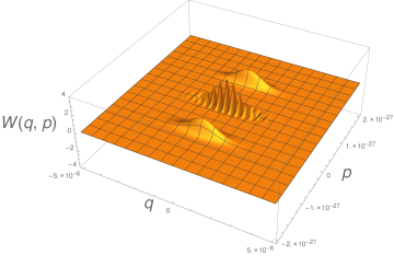
Figure 3: Figure shows a plot of the function $W(q,p)$ (defined in the text) as a function of $q$ and $p$ at $t=1\mu$ sec. The central hump showing oscillations is the real part of the off-diagonal element of the Wigner matrix and the others are diagonal elements. The remaining parameters and axes units are as mentioned in the caption of Fig. 2. The $W(q,p)$ axis has been rescaled by multiplying by a factor of $10^{-33}$. $q$ is displayed in $m$ and $p$ in $kgm/s$.

Figure 4: Figure shows a plot of the function $W(q,p,t)$ (defined in the text) as a function of $q$ and $p$ at t=30$\mu$ sec. The remaining parameters are as mentioned in the caption of Fig. 2. The $W(q,p)$ axis has been rescaled by multiplying by a factor of $10^{-33}$. $q$ is displayed in $m$ and $p$ in $kgm/s$.

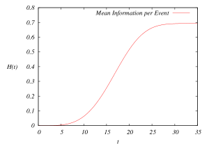
Figure 5: Mean information per event $\cal H$ versus time in $\mu$sec. The remaining parameters are as mentioned in the caption of Fig.2.

$${\cal H}=\int{P(X)I(X)dX} = \log{2}-\int{P(x)\log{P(x)}dx}$$ (13)

$$+\int{P_{+}(x)\log{P_{+}(x)}dx}$$

$$+\int{P_{-}(x)\log{P_{-}(x)}dx}.$$

At any time, $\cal H$ cannot of course exceed $S_{ent}$ the entanglement entropy, which is the maximum possible information that can be gained about the spin, by interrogating the position variable. It follows from Eq.(13) that ${\cal H}$ starts out from zero at $t=0$ and approaches $\log 2$ over a timescale of $\tau_{1}=10^{-5}{\rm s}$ (See Fig. 5). The fact that ${\cal H}$ is positive means that we do gain some information about the spin of the atoms by detecting their positions, even before the two wave packets have separated cleanly. After the wave packets have separated, the coherence between the two wavepackets is still manifest in the Wigner function. As is well known, the Wigner function is only a quasiprobability distribution. On coarse graining it becomes positive[10] and can be viewed as a probability distribution in the phase space of the atomic position. This constitutes coarse measurement.

5 Conclusion

In this letter we have addressed the Quantum Measurement Process in the context of the Stern-Gerlach experiment. An exact solution of the Schrödinger equation permits us to analyse unitary evolution in an idealised mathematical model of the experiment. Coarse Quantum Measurement (CQM) is based on the idea that every measurement is done with limited resources of resolution. The key conclusion of our analysis is that, the apparent loss of unitarity in a quantum measurement is a consequence of the coarseness of the experimental probes. Previous literature on coarse measurements [10, 11, 12] has not applied the idea to understand the classic Stern-Gerlach experiment which is of great interest as a paradigm for quantum measurement.

In the context of statistical mechanics, the authors of Ref. [18, 19] note that entropy is a subjective notion depending upon the resources available to the experimenter, to distinguish between statistical states. This follows the Bayesian approach to probability theory. The view we advocate is very similar in the context of quantum mechanics. The idea of “coarse measurement” is clearly a subjective one. Depending on the resources available to the experimenter, the evolution may appear unitary or otherwise. Thus, with a high enough resolution one can always detect interference effects. When the interference between the two wave packets is detectable, we must conclude that the spin is both up and down simultaneously. This does not constitute a measurement of the spin component $\sigma_{y}$. In a low resolution experiment, the interference apparently gets washed out and we can obtain information about the spin. This is the regime of interest in this letter.

Some of the quantum measurement literature concerns itself with von Neuman measurements, which can be regarded as instantaneous. One talks about “before” and “after” the measurement, but not during. Exceptions are weak[20] and nonideal measurements[21]. In weak measurements one tries to continuously extract information from a quantum system causing minimal disturbance using a weak probe, that does not destroy the interference pattern. In coarse measurements, one explicitly loses the interference pattern. Regarding non-ideal measurements Ref. [21] discusses the subtleties in the notion of distinguishability of apparatus states: even states which are orthogonal in the Hilbert space sense can have considerable spatial overlap. In contrast, our focus is on how a coarse measurement results in the apparent loss of coherence of the final wavepacket in a Stern-Gerlach setup. As has been emphasized by Ref. [10], the coarse measurement approach is conceptually different from the decoherence paradigm. Decoherence involves interaction with environmental degrees of freedom. Information is lost from the system by tracing over the environment. The coarse measurement approach does not invoke new degrees of freedom or new dynamics. It is essentially kinematical, dealing with the experimenter’s inability to measure or control fine details.

There have been other parallel developments [22, 23] which address the issue of imperfect measurements. In [22] the authors model the detector as a phase randomizer or dephaser, which leads to a mixed state density matrix starting from a pure state density matrix. In [23], the formalism of coarse-graining has been framed in a formal mathematical language. We go beyond this discussion by providing a physical basis in terms of resource limitation. Ref. [23] also touches upon the issue of non-idealness as in Ref. [21]. There has even been a suggestion [24] that the “reduction of the wavepacket” happens just when the atom enters the magnetic field.

In the actual experimental setup for the Stern-Gerlach experiment the atoms are heated in an oven to about $450K$. At this temperature, the two spin states of the silver atom are in an incoherent or classical superposition of the two spin states. As a result, the interference effects dealt with here will not be visible. To see the quantum interference effects discussed here, the internal state of the atom must be in a coherent superposition of spin states. An optical analog of the Stern-Gerlach experiment[25] may be a more practical candidate for realizing this experiment.

6 Acknowledgements

It is a pleasure to thank Patrick Dasgupta, N. D. Hari Dass, Anupam Garg, Chitrabhanu P., Karthik H. S., Gordon Love and Rafael Sorkin for stimulating discussions. We thank U. Sinha for drawing our attention to Ref.[21]

Appendix A Propagator For The Stern-Gerlach Setup

We consider a Stern-Gerlach setup with a magnetic field $\boldsymbol{B}=(B_{0}y,B_{0}x,0)$. The Hamiltonian for the problem is:

$$H=\frac{{p}^{2}}{2m}-\boldsymbol{{\mu}.{B}}$$ (A-1)

with $\boldsymbol{\mu}=g\mu_{B}\frac{\hbar}{2}{\boldsymbol{\sigma}}$ and the stationary solution satisfies:

$$H\psi=E\psi\,\left(\psi=\psi(x,z),\,\psi(x,0)=e^{-\frac{x^{2}}{2\sigma^{2}}}\right)$$ (A-2)

Restricting to the $x$-$z$ plane by setting $y=0$, the Hamiltonian can be written more explicitly as

$$H=\frac{p_{x}^{2}+p_{z}^{2}}{2m}+xF\sigma_{y}$$ (A-3)

where, $F=-g\mu_{B}\frac{\hbar}{2}B_{0}$ and if we assume a solution of the form $\psi(x,z)=\phi(x,z)\,e^{ikz}$ (since this is a propagating wave along z-direction), Eq.(A-2) in the paraxial approximation reduces to the following:

$$i\hbar\left(\frac{k\hbar}{m}\right)\frac{\partial\phi}{\partial z}=-\frac{\hbar^{2}}{2m}\frac{\partial^{2}\phi}{\partial x^{2}}+xF\sigma_{y}\phi$$ (A-4)

if we set $E=\frac{k^{2}\hbar^{2}}{2m}$.

This equation can be identified with the time dependent Schrödinger equation, by setting $t=\frac{zm}{k\hbar}$:

$$i\hbar\frac{\partial\phi}{\partial t}=-\frac{\hbar^{2}}{2m}\frac{\partial^{2}\phi}{\partial x^{2}}+xF\sigma_{y}\phi$$ (A-5)

Since the eigenvalues of $\sigma_{y}$ are +1 and -1 we get the corresponding components of the spinor $\phi$ as $\phi_{+}$ and $\phi_{-}$, respectively. Thus Eq.(5) reduces to:

$$i\hbar\frac{\partial\phi_{+}}{\partial t}=-\frac{\hbar^{2}}{2m}\frac{\partial^{2}\phi_{+}}{\partial x^{2}}+xF\phi_{+}$$ (A-6)

$$i\hbar\frac{\partial\phi_{-}}{\partial t}=-\frac{\hbar^{2}}{2m}\frac{\partial^{2}\phi_{-}}{\partial x^{2}}-xF\phi_{-}$$ (A-7)

To solve these equations we move to an accelerated frame along the x-axis and employ the following transformations in $x$, $t$ and $\phi$, which reduce the above equations to a free particle equation for $\tilde{\phi}_{\pm}(\xi,T)$ where $\xi$ is related to $x$ as follows:

$$x=\xi\pm\frac{1}{2}aT^{2}\\$$ (A-8)

and

$$t=T\\$$ (A-9)

Thus we have:

$$\phi_{\pm}(x,t)=\tilde{\phi}_{\pm}(\xi,T)\,e^{if(\xi,T)}$$ (A-10)

We outline the solution to Eq.(A-6).Substituting Eqs. (A-8), (A-9) and (A-10) in Eq.(A-6) we reduce Eq.(A-6) to a free particle equation and find $f$ and $a$ :

$$f=\frac{maT}{\hbar}(\xi+\frac{1}{3}aT^{2}),\,a=-\frac{F}{m}$$ (A-11)

The kernel (propagator) for the free particle problem corresponding to Eq.(A-6) is:

$$\tilde{K}(x,x_{i};t)=\sqrt{\frac{m}{2\pi i\hbar t}}\ e^{\,\displaystyle i\frac{m(x-x_{i})^{2}}{2\hbar t}}$$ (A-12)

where $x$ is the position at time $t$ and $x_{i}$ is position at $t_{i}=0$. We can find the propagator for the Hamiltonian under consideration by applying the following transformation.

$$K(x,x_{i};t)=e^{if(x,t)}\tilde{K}(x,x_{i};t)$$ (A-13)

which gives Eq.(5) of the main text:

$$K^{{}^{++}}(x,x_{i};t)=\sqrt{\frac{m}{2\pi i\hbar t}}\text{exp}\left\{i\left(\frac{m}{2\hbar t}(x-x_{i})^{2}-\frac{Ft}{2\hbar}(x+x_{i})-\frac{F^{2}t^{3}}{24m\hbar}\right)\right\}$$ (A-14)

The solution to Eq.(A-6) can be cast as follows:

$$\phi_{+}(x,t)=\int_{-\infty}^{\infty}K^{++}(x,x_{i},t)\,\phi_{+}(x_{i},0)\,dx_{i}$$ (A-15)

After solving Eq.(A-13) we get the final solution for $\phi_{+}$. We employ the same procedure to find $\phi_{-}$. The solutions are:

In general, one can consider a further evolution beyond the region where the magnetic field is present and consider free evolution which leads to solutions of the form given below:

where $t_{1}$ is the amount of time spent by the atom in the magnetic field and $t$ is the total time of evolution.

Appendix B Suppression of off diagonal elements of the Wigner matrix due to coarse graining

The Wigner matrix is of the form:

$$\mathbf{W}(q,p)=\left(\begin{array}[]{cc}W_{++}(q,p)&W_{+-}(q,p)\\ W_{-+}(q,p)&W_{--}(q,p)\end{array}\right)$$ (B-1)

Explicitly, for instance, we have:

$$W_{+-}(q,p)={\frac{1}{2\pi\hbar}}\text{exp}\left[-\left\{\frac{(pt-mq)^{2}}{m^{2}\sigma^{2}}+\frac{p^{2}\sigma^{2}}{\hbar^{2}}+\frac{iat(pt-2mq)}{\hbar}\right\}\right]$$ (B-3)

Notice that $W_{+-}(q,p)$ oscillates on a spatial scale $d=\frac{\hbar}{2mat}=\frac{\hbar}{2Ft}$. The coarse grained Wigner matrix $\overline{\mathbf{W}}(q,p)$ has elements

$$\overline{W}_{\alpha\beta}(q,p)=\frac{1}{\Delta\delta}\int_{-\Delta/2}^{\Delta/2}du\int_{-\delta/2}^{\delta/2}dv{W}_{\alpha\beta}(q+u,p+v),$$ (B-4)

with $\Delta$ and $\delta$, the pixel size in position and momentum respectively. The numerically generated plots show how the offdiagonal terms ${W}_{+-}(q,p)$ and ${W}_{-+}(q,p)$ on coarse graining average to zero due to the presence of the oscillatory term $e^{iq\frac{2\pi}{d}}$, where $d$ is the spatial scale of oscillation. We finally get the following diagonal form for the coarse grained Wigner matrix:

$\left(\begin{array}[]{ccc}\overline{W}_{++}(q,p)&0\\ &&\\ 0&\overline{W}_{--}(q,p)\end{array}\right)$

For instance, for $q=10^{-6}m$ and $p=0kgm/s$ and $t=3\times 10^{-5}s$ we get the following form for the coarse grained Wigner matrix, for the realistic experimental parameter values for a typical Stern Gerlach setup.

$$\overline{\mathbf{W}}(q,p)=\left(\begin{array}[]{cc}5.7\times 10^{-2}&0\\ 0&1.6\times 10^{-5}\end{array}\right)$$ (B-5)

References

- [1] A. Venugopalan, D. Kumar, R. Ghosh, Environment-induced decoherence i. the stern-gerlach measurement, Physica A: Statistical Mechanics and its Applications 220 (3–4) (1995) 563 – 575. doi:http://dx.doi.org/10.1016/0378-4371(95)00184-9.
- [2] A. Venugopalan, Decoherence and schrödinger-cat states in a stern-gerlach-type experiment, Phys. Rev. A 56 (1997) 4307–4310. doi:10.1103/PhysRevA.56.4307.
- [3] M. Gondran, A. Gondran, A complete analysis of the stern-gerlach experiment using pauli spinors, arXiv preprint quant-ph/0511276.
- [4] M. Hannout, S. Hoyt, A. Kryowonos, A. Widom, Quantum measurement theory and the stern–gerlach experiment, American Journal of Physics 66 (5).
- [5] D. E. Platt, A modern analysis of the Stern-Gerlach experiment, American Journal of Physics 60 (1992) 306–308. doi:10.1119/1.17136.
- [6] G. P. Berman, G. D. Doolen, P. C. Hammel, V. I. Tsifrinovich, Static stern-gerlach effect in magnetic force microscopy, Phys. Rev. A 65 (2002) 032311. doi:10.1103/PhysRevA.65.032311.
- [7] M. Frasca, Stern-gerlach experiment and bohm limit, arXiv preprint quant-ph/0402072.
- [8] M. O. Scully, E. L. Willis, A. Barut, On the theory of the stern-gerlach apparatus, Foundations Of Physics 17 (1987) 575.
- [9] P. Gomis, A. Pérez, A study of decoherence effects in the Stern-Gerlach experiment using matrix Wigner functions, arXiv preprint quant-ph/1507.08541arXiv:1507.08541.
- [10] J. Kofler, C. Brukner, Classical world arising out of quantum physics under the restriction of coarse-grained measurements, Phys. Rev. Lett. 99 (2007) 180403. doi:10.1103/PhysRevLett.99.180403.
- [11] H. Jeong, Y. Lim, M. S. Kim, Coarsening measurement references and the quantum-to-classical transition, Phys. Rev. Lett. 112 (2014) 010402. doi:10.1103/PhysRevLett.112.010402.
- [12] S. Raeisi, P. Sekatski, C. Simon, Coarse graining makes it hard to see micro-macro entanglement, Phys. Rev. Lett. 107 (2011) 250401. doi:10.1103/PhysRevLett.107.250401.
- [13] M. Steiner, M. Frey, A. Gulian, R. W. Rendell, A. K. Rajagopal, Measurement of a subsystem of a coupled quantum system (2009). doi:10.1117/12.817558.
- [14] B. C. Hsu, M. Berrondo, J.-F. m. c. S. Van Huele, Stern-gerlach dynamics with quantum propagators, Phys. Rev. A 83 (2011) 012109. doi:10.1103/PhysRevA.83.012109.
- [15] R. Feynman, A. R. Hibbs, Quantum Mechanics and Path Integrals, McGraw-Hill, 1965.
-
[16]
R. Horodecki, P. Horodecki, M. Horodecki, K. Horodecki,