Liquid relaxation: A new Parodi-like relation for nematic liquid crystals

Abstract

We put forward a hydrodynamic theory of nematic liquid crystals that includes both anisotropic elasticity and dynamic relaxation. Liquid remodeling is encompassed through a continuous update of the shear-stress free configuration. The low-frequency limit of the dynamical theory reproduces the classical Ericksen-Leslie theory, but it predicts two independent identities between the six Leslie viscosity coefficients. One replicates Parodi’s relation, while the other—which involves five Leslie viscosities in a nonlinear way—is new. We discuss its significance, and we test its validity against evidence from physical experiments, independent theoretical predictions, and molecular-dynamics simulations.

I Introduction

Liquids are unable to sustain any nonzero stationary shear stress. In ordinary conditions—i.e., at small enough strain rates—shear relaxation occurs exponentially fast, producing a viscoelastic analog of the dielectric Debye relaxation. However, at the crossover between the characteristic shearing time and the liquid relaxation time 47fre , distinctive solidlike features become increasingly manifest 85hido07tra12bflrt . Molecular rearrangements are dramatically slowed down in confined ultrathin liquid films (three to ten molecular dimensions thick), whose relaxation times may be as large as tens to hundreds of milliseconds 91hcg , making the crossover more experimentally accessible. But clear fingerprints of a smooth transition from liquidlike to solidlike response manifest also in the acoustic properties of nematic liquid crystals (NLCs) in the MHz–GHz frequency range 95gr&95kr&99ruo&12kkkk .

In this paper we show how a fairly general continuum theory of liquids may be established by allowing the effective shear strain—i.e., the shear strain from an evolving relaxed configuration—to enter the strain energy functional. A dissipation principle governs the evolution of such a configuration, and it takes into account the macroscopic effects of microscopic rearrangements 02diq04rasi . In a previous work 14bdt15tur , we constructed such a theory for (slightly) compressible NLCs and applied it, with fair success, to explain quantitatively the anisotropy of sound velocity 72muls and sound attenuation 70lordlab in $N$-(4-methoxybenzylidene)-4-butylaniline (MBBA) over the range 2–14 MHz. The theory of nematic relaxation put forth in 14bdt15tur is characterized by: (i) a neo-Hookean contribution to the strain energy where the effective shear strain enters weighted by an anisotropic shape tensor, and (ii) an isotropic gradient flow dynamics for the relaxed configuration, parameterized by a single viscosity modulus. Here we keep (i) as is, but we revise and extend (ii) by taking a gradient flow with respect to an anisotropic metric possessing the minimum symmetry compatible with the liquid crystal. This theory covers the whole range from low-frequency hydrodynamics to solidlike high-frequency regimes 95gr&95kr&99ruo&12kkkk . In particular, the low-frequency predictions reproduce the well-known Ericksen-Leslie 60eri ; 68lesl dynamical theory, but they deliver in addition a new Parodi-like relation between viscosity coefficients. Along with the original Parodi relation 70paro —which we also retrieve—this result lowers to four the number of independent viscosities for a nematic liquid crystal. Both conditions involve only (some of) the six original Leslie coefficients, not the extra three viscosities entering the extension of the Ericksen-Leslie theory to compressible NLCs 75mon& . Accordingly, only the theory for incompressible NLCs will be presented here, and its predictions tested against experimental data, earlier theoretical predictions, and results from molecular-dynamics (MD) simulations. The discussion of the compressible case is left to a future paper.

II Relaxational dynamics

We briefly sketch the theory that provides the equations of motion for a NLC, under the combined effect of anisotropic elasticity and anisotropic relaxation. Let $\mathbf{F}$ be the deformation gradient from an arbitrarily selected reference configuration of the NLC body. To account for relaxation, we factorize $\mathbf{F}$ into a relaxing deformation $\mathbf{G}$ and an effective deformation $\mathbf{F}_{\!\mathsf{e}}$:

$$\mathbf{F}\!=\!\mathbf{F}_{\!\mathsf{e}}\mathbf{G}\,,$$ (1)

with $\mathbf{G}$ identifying the relaxed equilibrium configuration, and the effective deformation $\mathbf{F}_{\!\mathsf{e}}$ measuring the deviation from equilibrium of the current deformation. Consequently, only the effective deformation enters the strain energy. Since $\mathbf{F}_{\!\mathsf{e}}\!=\!\mathbf{F}\mathbf{G}^{-1}$ maps from the relaxed to the current configuration, the strain energy is properly defined, being independent of the arbitrarily chosen reference. For an incompressible NLC, all factors in (1) are isochoric, i.e., have unit determinant.

In order to account for anisotropic elasticity, we augment the classical Oseen-Frank O-F free-energy density (per unit volume) with the anisotropic potential

$$\Upsilon_{\!\mathsf{shr}}=\tfrac{1}{2}\mu\operatorname{tr}(\bm{\Psi}^{-1}\mathbf{B}_{\mathrm{e}}-\mathbf{I}),$$ (2)

where $\mu$ is the shear modulus. The strain energy (2) simply measures the deviation of the effective strain $\mathbf{B}_{\mathrm{e}}\,\raise 0.32224pt\hbox{:}\kern-0.24994pt\hbox{=}\,\mathbf{F}_{\!\mathsf{e}}\mathbf{F}_{\!\mathsf{e}}^{\top}$ from the energetic shape tensor

$$\bm{\Psi}\,\raise 0.32224pt\hbox{:}\kern-0.24994pt\hbox{=}\,a^{2}(\mathbf{n}\operatorname{\otimes}\mathbf{n})+a^{-1}(\mathbf{I}-\mathbf{n}\operatorname{\otimes}\mathbf{n}),$$ (3)

parameterized by the aspect ratio $a\!>\!0$, whose deviation from $1$ gauges the degree and the type (prolate or oblate) of elastic anisotropy with respect to the nematic director $\mathbf{n}$ ratio . The shape tensor $\bm{\Psi}$ is symmetric, positive definite, and with unit determinant. The potential $\Upsilon_{\!\mathsf{shr}}$ adds the following contribution to the stress tensor 14bdt15tur ; dev :

$$\mathbf{T}_{\mathsf{shr}}\!=\!\mu\operatorname{dev}(\bm{\Psi}^{-1}\mathbf{B}_{\mathrm{e}}).$$ (4)

Clearly, $\mathbf{T}_{\mathsf{shr}}$ vanishes if and only if $\mathbf{B}_{\mathrm{e}}\!=\!\bm{\Psi}$, where $\Upsilon_{\!\mathsf{shr}}$ attains its unique minimum.

We now proceed to derive an evolution equation for the relaxing deformation $\mathbf{G}$. Since $\mathbf{B}_{\mathrm{e}}\!=\mathbf{F}\mathbf{H}\mathbf{F}^{\top}\!$, with the inverse relaxing strain defined as $\mathbf{H}\,\raise 0.32224pt\hbox{:}\kern-0.24994pt\hbox{=}\,(\mathbf{G}^{\top}\mathbf{G})^{-1}$, the strain energy density (2) depends on the relaxing deformation $\mathbf{G}$ only through $\mathbf{H}$. Any relaxation dynamics necessarily obeys a dissipation inequality, ensuring a nonnegative entropy production. In this case, such an inequality reads

$$\big{(}\mathbf{F}^{\!\top}\bm{\Psi}^{-1}\mathbf{F}\big{)}\!\cdot\!\dot{\mathbf{H}}\leq 0$$ (5)

(see 14bdt15tur ). In terms of the co-deformational derivative

$$\mathbf{B}_{\mathrm{e}}^{\!\blacktriangledown}\,\raise 0.32224pt\hbox{:}\kern-0.24994pt\hbox{=}\,\dot{\mathbf{B}}_{\mathsf{e}}-(\bm{\nabla}\mathbf{v})\,\mathbf{B}_{\mathrm{e}}-\mathbf{B}_{\mathrm{e}}(\bm{\nabla}\mathbf{v})^{\!\top}\!=\,\mathbf{F}\overset{\bm{.}}{\mathbf{H}}\mathbf{F}^{\top}\!,$$ (6)

where $\mathbf{v}$ is the translational velocity field and $\bm{\nabla}\mathbf{v}\!=\!\dot{\mathbf{F}}\mathbf{F}^{-1}$ is its spatial gradient, inequality (5) takes the form

$$\bm{\Psi}^{-1}\!\cdot\mathbf{B}_{\mathrm{e}}^{\!\blacktriangledown}\!<0\quad\textrm{unless}\quad\mathbf{B}_{\mathrm{e}}^{\!\blacktriangledown}\!=0\,,$$ (7)

made stricter by the presumption that relaxation does dissipate. The simplest way to satisfy it is to assume that there is an invertible dissipation tensor $\mathbb{D}$ whose symmetric part is positive definite, such that

$$\mathbb{D}\,\mathbf{B}_{\mathrm{e}}^{\!\blacktriangledown}=-\,\bm{\Psi}^{-1}+\lambda\,\mathbf{B}_{\mathrm{e}}^{-1},$$ (8)

where the Lagrange multiplier $\lambda$ enforces the condition that the relaxation process be isochoric. After introducing the mobility tensor $\,\mathbb{M}\,\raise 0.32224pt\hbox{:}\kern-0.24994pt\hbox{=}\,\mathbb{D}^{-1}$, this yields the gradient-flow equation IP

$$\mathbf{B}_{\mathrm{e}}^{\!\blacktriangledown}=-\,\mathbb{M}\!\left(\!\bm{\Psi}^{-1}-\frac{(\mathbb{M}\,\bm{\Psi}^{-1})\!\cdot\!\mathbf{B}_{\mathrm{e}}^{-1}}{(\mathbb{M}\,\mathbf{B}_{\mathrm{e}}^{-1})\!\cdot\!\mathbf{B}_{\mathrm{e}}^{-1}}\,\mathbf{B}_{\mathrm{e}}^{-1}\!\right)\!.$$ (9)

Note that, contrary to $\mathbf{H}$, the effective strain $\mathbf{B}_{\mathrm{e}}$ is independent of the arbitrarily chosen reference. Hence, the relaxation dynamics (9) is properly defined.

The most general dissipation tensor $\mathbb{D}$ sharing the symmetry of the shape tensor (3) may be parameterized by six scalar coefficients $\tau_{1},\dots,\tau_{6}$, as 87povi

$$\mathbb{D}\,\mathbf{L} =\tau_{1}\mathbf{L}+\tau_{2}(\operatorname{tr}\mathbf{L})\,\mathbf{I}+\tau_{3}(\bm{\Psi}\mathbf{L}+\mathbf{L}\bm{\Psi})$$ (10)

$$\,+\tau_{4}\big{(}(\operatorname{tr}\mathbf{L})\bm{\Psi}+(\bm{\Psi}\!\cdot\!\mathbf{L})\,\mathbf{I}\,\big{)}+\tau_{5}\bm{\Psi}\mathbf{L}\bm{\Psi}$$

$$\,+\tau_{6}\big{(}(\operatorname{tr}\mathbf{L})\bm{\Psi}-(\bm{\Psi}\!\cdot\!\mathbf{L})\,\mathbf{I}\,\big{)},\quad\text{for all }\mathbf{L}\in\text{Sym}.$$

It depends on the aspect ratio $a$ via $\bm{\Psi}$, and possibly also via the coefficients $\tau_{1},\dots,\tau_{6}$. Generically, $\mathbb{D}$ has two double eigenvalues:

$$\tau_{\perp} =\tau_{1}+(a^{2}\!+a^{-1})\tau_{3}+a\,\tau_{5}>0\,,$$ (11)

$$\tau_{\|} =\tau_{1}+2\,a^{-1}\,\tau_{3}+a^{-2}\,\tau_{5}>0\,,$$

associated respectively with the shearing modes in the plane normal to $\mathbf{n}$ and the shearing modes that tilt the nematic director. Their inverses measure how fast these modes relax. On the (complementary) invariant subspace spanned by the orthonormal pair $\big{(}(\sqrt{3}/2)\operatorname{dev}(\mathbf{n}\!\otimes\!\mathbf{n})$, $(1/\sqrt{3}\,)\mathbf{I}\big{)}$, $\mathbb{D}$ acts as follows

$$[\,\mathbb{D}\,]=\begin{pmatrix}\tau_{11}&\tau_{12}\\ \tau_{21}&\tau_{22}\end{pmatrix},$$

where

$$\tau_{11}=\tau_{1}+\frac{4\,a^{3}+2}{3\,a}\,\tau_{3}+\frac{2\,a^{6}+1}{3\,a^{2}}\,\tau_{5}\,,$$

$$\tau_{22}=\tau_{1}+3\,\tau_{2}+2\,\frac{a^{3}+2}{3\,a}\,\tau_{3}+2\,\frac{a^{3}+2}{a}\,\tau_{4}+\frac{a^{6}+2}{3\,a^{2}}\,\tau_{5}\,,$$

$$\tfrac{1}{2}(\tau_{12}+\tau_{21})=\sqrt{2}\,\frac{a^{3}-1}{3a^{2}}\big{(}2\,a\,\tau_{2}+3\,a\,\tau_{4}+(1+a^{3})\,\tau_{5}\big{)}\,,$$

$$\tfrac{1}{2}(\tau_{12}-\tau_{21})=\sqrt{2}\,\frac{a^{3}-1}{a}\,\tau_{6}\,.$$

with

$$\tau_{11}\tau_{22}-\tfrac{1}{4}\big{(}\tau_{12}+\tau_{21}\big{)}^{2}>0\,.$$ (12)

Under positivity conditions (11) and (12), $\mathbb{D}$ is invertible whatever the value of $\tau_{6}$ is. For $a\!=\!1$ (a condition identifying an isotropic liquid), $\tau_{\perp}$ and $\tau_{\|}$ collapse into $\tau_{11}\!=\tau_{1}\!+2\,\tau_{3}+\tau_{5}\!>0\,$, $\tau_{12}\!=\tau_{21}\!=0\,$, and (10) reduces to

$$\mathbb{D}\,\mathbf{L}=\tau_{11}\operatorname{dev}\mathbf{L}+\tau_{22}\,\tfrac{1}{3}(\operatorname{tr}\mathbf{L})\mathbf{I}\,,$$

with $\tau_{22}=\tau_{11}\!+3\,(\tau_{2}+2\,\tau_{4})>0\,$.

III Low-frequency limit: a new Parodi relation

Now that we have characterized both the elastic and the relaxational material properties, we set up a perturbative procedure fit to study the slow motions where the system is expected to comply with the Ericksen-Leslie hydrodynamics. The evolution equation (9) has only one stationary solution: $\mathbf{B}_{\mathrm{e}}\!=\!\bm{\Psi}$, which is globally attractive. Therefore, if the deformation process is slow enough (on the time scale set by the largest relaxation time characterizing $\mathbb{D}$), the ensuing viscous response is well described by linearizing the right side of (9) about $\bm{\Psi}$ and assuming the deformation gradient to be retarded in the sense of Col&Noll :

$${}_{\varepsilon}\mathbf{F}_{\!\mathrm{e}}(t)\,\raise 0.32224pt\hbox{:}\kern-0.24994pt\hbox{=}\,\mathbf{F}^{(0)}_{\!\mathrm{e}}(\varepsilon\,t)+\varepsilon\,\mathbf{F}^{(1)}_{\!\mathrm{e}}(\varepsilon\,t)+o(\varepsilon)\mathbf{F}^{(+)}_{\!\mathrm{e}}(\varepsilon\,t)\,,$$ (13)

implying that ${}_{\varepsilon}\dot{\mathbf{F}}_{\!\mathsf{e}}\!=\varepsilon\,\dot{\mathbf{F}}^{(0)}_{\!\mathrm{e}}\!+o(\varepsilon)$ and ${}_{\varepsilon}\mathbf{B}_{\mathrm{e}}^{\!\blacktriangledown}=\varepsilon\,\bm{\Psi}^{\!\blacktriangledown}\!+o(\varepsilon)$. Under these assumptions, equation (9), trivially satisfied at $O(1)$, at $O(\varepsilon)$ leads to

$$\operatorname{dev}\!\big{(}\bm{\Psi}^{-1}\mathbf{B}^{(1)}_{\mathrm{e}}\big{)}=-\operatorname{dev}\!\big{(}(\mathbb{D}\,\bm{\Psi}^{\!\blacktriangledown})\bm{\Psi}\big{)},$$ (14)

which, substituted into (4), yields

$$\mathbf{T}_{\mathsf{shr}}^{(1)}\!=\!-\mu\operatorname{dev}\!\big{(}(\mathbb{D}\,\bm{\Psi}^{\!\blacktriangledown})\bm{\Psi}\big{)}.$$ (15)

The co-deformational derivative of the shape tensor (3) reads

$$\bm{\Psi}^{\!\blacktriangledown} \,\raise 0.32224pt\hbox{:}\kern-0.24994pt\hbox{=}\,\dot{\bm{\Psi}}-(\bm{\nabla}\mathbf{v})\,\bm{\Psi}-\bm{\Psi}(\bm{\nabla}\mathbf{v})^{\!\top}$$

$$=2\!\left(a^{2}\!-a^{-1}\right)\operatorname{sym}\!\big{(}\mathbf{\mathring{n}}\!\otimes\!\mathbf{n}-(\mathbf{D}\mathbf{n})\!\otimes\!\mathbf{n}\big{)}-2\,a^{-1}\mathbf{D}\,,$$

where $\mathbf{\mathring{n}}\,\raise 0.32224pt\hbox{:}\kern-0.24994pt\hbox{=}\,\dot{\mathbf{n}}-\mathbf{W}\mathbf{n}$ is the co-rotational derivative of the nematic director, $\mathbf{D}\,\raise 0.32224pt\hbox{:}\kern-0.24994pt\hbox{=}\,\operatorname{sym}(\bm{\nabla}\mathbf{v})$ the (traceless) stretching, and $\mathbf{W}\,\raise 0.32224pt\hbox{:}\kern-0.24994pt\hbox{=}\,\operatorname{skw}(\bm{\nabla}\mathbf{v})$ is the spin.

We are now in a position to compare our result (15) with the most general linear viscous stress compatible with the nematic structure, as posited in 68lesl , namely

$$\alpha_{1}\mathbf{n}\!\cdot\!(\mathbf{D}\mathbf{n})\mathbf{n}\!\operatorname{\otimes}\!\mathbf{n}+\alpha_{2}\mathbf{\mathring{n}}\!\operatorname{\otimes}\!\mathbf{n}+\alpha_{3}\mathbf{n}\!\operatorname{\otimes}\!\mathbf{\mathring{n}}$$ (16)

$$\,+\,\alpha_{4}\mathbf{D}+\alpha_{5}(\mathbf{D}\mathbf{n})\!\operatorname{\otimes}\!\mathbf{n}+\alpha_{6}\mathbf{n}\!\operatorname{\otimes}(\mathbf{D}\mathbf{n})\,,$$

whose traceless component matches (15) provided that the six Leslie viscosities are identified as follows:

$$\alpha_{1} =\mu\,a^{-3}\big{[}2\,(a^{3}-1)^{2}\,\big{(}a^{7}\tau_{1}+a\,\tau_{2}+2\,(a^{3}+1)\,\tau_{4}\big{)}$$

$$+a\,(4\,a^{9}-a^{6}-2\,a^{3}-1)\,\tau_{\perp}\!-2\,a\,(a^{12}-1)\,\tau_{\|}\big{]},$$

$$\alpha_{2} =-\mu\,(a^{3}\!-1)\,a\,\tau_{\perp},$$

$$\alpha_{3} =-\mu\,(a^{3}\!-1)\,a^{-2}\,\tau_{\perp},$$ (17)

$$\alpha_{4} =2\,\mu\,a^{-2}\,\tau_{\|},$$

$$\alpha_{5} =\mu\big{(}(a^{3}\!+1)\,a\,\tau_{\perp}-2\,a^{-2}\,\tau_{\|}\big{)},$$

$$\alpha_{6} =\mu\big{(}(a^{3}\!+1)\,a^{-2}\,\tau_{\perp}-2\,a^{-2}\,\tau_{\|}\big{)}.$$

These viscosity coefficients satisfy identically the well-known Parodi relation 70paro

$$\alpha_{2}+\alpha_{3}=\alpha_{6}-\alpha_{5}\,.$$ (18)

This should be expected, since $\tau_{6}$, the only coefficient breaking the symmetry of $\mathbb{D}$, does not enter equalities (17) tau6 . A far less obvious result is the new nonlinear relation involving all Leslie viscosities but $\alpha_{1}$:

$$\frac{\alpha_{2}}{\alpha_{3}}=\frac{\alpha_{4}+\alpha_{5}}{\alpha_{4}+\alpha_{6}}\,,$$ (19)

and the fact that the cubic root of the two ratios equated in (19) equals the aspect ratio $a$:

$$\frac{\alpha_{2}}{\alpha_{3}}=\frac{\alpha_{4}+\alpha_{5}}{\alpha_{4}+\alpha_{6}}=a^{3}.$$ (20)

For $a\!=\!1$ (implying $\bm{\Psi}\!=\!\mathbf{I}$ and an isotropic free-energy density), all $\alpha$’s vanish but $\alpha_{4}\!=2\,\mu\,\tau_{11}$. The ratio $\alpha_{2}/\alpha_{3}$ is hence undefined. However, (19) and (20) still hold by continuity. Parodi’s relation (18), stemming from a general thermodynamic argument, is so well established that it is simply taken for granted by experimentalists who identify all of the six Leslie coefficients in the absence of data from normal stress measurements 79Leslie . The new relation (19), on the contrary, is specific to the present theory of anisotropic nematic relaxation. Checking (19) against evidence from independent sources provides therefore a significant test of our theory.

To do so, we have at our disposal both experimental and theoretical results, along with numerical simulations. More precisely, in what follows we analyze: (i) an early paper 88hess on MD simulation of NLCs, inspired by the model molecular theory put forward by Helfrich 69helf , and a relatively recent one 07wu , based on the Gay-Berne potential; (ii) the experimental study 82kneppe universally regarded as the standard reference for the viscosities of MBBA between $20$ and $44^{\circ}$C; (iii) the outcome of a study on non-equilibrium statistical mechanics initiated by Osipov and Terentjev NESM ; Chrza& , extending previous results by Kuzuu and Doi Kuzuu&Doi (see, in particular, the recent comprehensive review by Chan and Terentjev NESM ).

In 88hess , Baals and Hess computed a complete set of viscosity coefficients by running a series of non-equilibrium MD simulations on a small system comprised of 128 particles, interacting through either a Lennard-Jones ellipsoid or a soft ellipsoid (purely repulsive) potential and subjected to plane Couette flows with various shear rates and different orientations relative to the uniform nematic direction, which was kept fixed in all runs. Their results are immediately comparable with the predictions of our theory, both having been obtained for a perfectly aligned nematic fluid. The coefficients in 88hess may hence enter directly the left and right sides of equality (19), which happens to be satisfied remarkably well (see Table 1).

All remaining data are obtained for partially oriented NCLs. Nematic viscosities depend on the degree of nematic order essentially through the scalar Maier-Saupe order parameter $S$, ranging from 0 (isotropic state) to 1 (perfect alignment) NESM ; Chrza& ; Kuzuu&Doi ; 88Lee;95ehhe;04sovi . To compensate for the fact that our theory does not account for partial order, we obtain a crude reconstruction of the nominal values of nematic viscosities at $S\!=\!1$ from values measured for partially ordered NLCs by replacing each $\mathbf{n}\!\operatorname{\otimes}\!\mathbf{n}$ term in the viscous stress (16) by the corresponding second-moment tensor $S\mathbf{n}\!\operatorname{\otimes}\!\mathbf{n}$ 88Lee;95ehhe;04sovi and taking into account that the nematic contribution to the shear viscosity $\alpha_{4}$ is overshadowed by a dominant isotropic contribution 82kneppe ; Chrza& .

In 07wu , Wu, Qian, and Zhang performed non-equilibrium MD simulations on a system of about 6,000 molecules, interacting via a Gay-Berne potential, for determining the six Leslie coefficients for each of three different shear rates. Their values, extrapolated from $S=0.75$ to $1$ through the above-described reconstruction procedure, show a striking agreement with relation (19) (see Table 1).

In 82kneppe , Kneppe et al. provided a complete set of Leslie coefficients for several temperature values ranging from $20$ to $44^{\circ}$C. Fig. 1 shows that the measured values may be satisfactorily fitted with our predictions (17), provided we assume that the Leslie viscosities depend on the Maier-Saupe order parameter $S$ as discussed above, and $S$ itself depends on temperature as in Table 2. A remarkable exception is provided by the Leslie coefficient $\alpha_{3}$, which deserves special attention. In fact, in 82kneppe the authors themselves raise a warning concerning this coefficient, which they derive as the difference of two nearly equal quantities, to the point that they hope for alternative measuring techniques. In particular, one of the striking peculiarities of the experimental $\alpha_{3}$ estimate in 82kneppe is that, at variance with all other viscosities, it appears to increase when the degree of orientation decreases. On the contrary, our theory predicts a consistent temperature dependence for all nematic viscosities.

$\Bigg{|}$​​Source	$\dfrac{\alpha_{2}}{\alpha_{3}}\Big{/}\dfrac{\alpha_{4}+\alpha_{5}}{\alpha_{4}+\alpha_{6}}$	$\dfrac{\alpha_{2}+\alpha_{3}}{\alpha_{6}-\alpha_{5}}$	$a$
88hess LJE	$1.01\pm 0.59$	$0.91\pm 0.41$	$1.75\pm 0.62$
​​88hess   SE	1.01 $\pm$ 0.45	1.01 $\pm$ 0.39	1.78 $\pm$ 0.57
07wu 0.066	0.92 $\pm$ 0.24	1.01 $\pm$ 0.06	2.02 $\pm$ 0.09
07wu 0.044	0.98 $\pm$ 0.30	1.04 $\pm$ 0.08	1.96 $\pm$ 0.10
07wu 0.022	1.10 $\pm$ 0.73	1.10 $\pm$ 0.20	1.94 $\pm$ 0.21

Table 1: LJE and SE stand respectively for Lennard-Jones ellipsoid and soft ellipsoid potentials, as used in 88hess ; the shear rates used in 07wu are given in L-J reduced units. The third column, relative to Parodi’s relation (18), is provided as a term of comparison. The scatter of the results from 88hess is huge, due to the small size of the molecular sample.

$\,T\,[^{\circ}\text{C}\,]$	20	25	30	35	40	42	44
$S$	0.92	0.66	0.48	0.34	0.23	0.19	0.14

Table 2: Values of the Maier-Saupe order parameter $S$ identified by a best fit between experimental MBBA viscosities in 82kneppe and our theory (see text for details). Note that the temperature dependence we obtain for $S$ is consistent with a weakly first-order nematic-isotropic phase transition, with a critical temperature $T_{\textrm{\tiny NI}}\simeq 49\,^{\circ}$C.

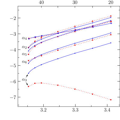
Figure 1: Viscosity coefficients of nematic MBBA as a function of temperature: our $S$-rescaled values (solid lines) vs. experimental data from 82kneppe (dotted lines). Bottom $x$-axis: inverse of absolute temperature (${\rm mK}^{-1}$); top $x$-axis: temperature (^∘C); $y$-axis: logarithm of the modulus of viscosities in Pa s (all of them negative, except $\alpha_{4}$ and $\alpha_{5}$).

A third and final test for our theoretical predictions comes from the non-equilibrium Fokker-Planck analysis developed in NESM ; Chrza& ; Kuzuu&Doi . This mean-field theory deals exclusively with the relaxational dynamics of the orientational degrees of freedom of anisotropic molecules to the exclusion of the translational relaxation associated with shear flow. Consequently, it does not provide reliable predictions for the shear viscosity coefficient $\alpha_{4}$, and therefore it cannot be used as a direct test for the new Parodi-like relation (19). Moreover, this theory delivers an explicit universal representation only for the symmetric part of the stress tensor, while the rotational viscosity $\gamma_{1}\!=\alpha_{3}-\alpha_{2}$ (and hence the complete set of Leslie viscosities) depends on the specific form of the assumed mean-field potential. That having been said, results in NESM ; Chrza& ; Kuzuu&Doi are in good qualitative agreement with our formulas (17)—with the obvious exception of $\alpha_{4}$.

Equality (20) further allows us to establish a direct link between the aspect ratio $a$—playing a key role in the present theory of nematic relaxation but not directly observable—and quantities amenable to experimental and numerical determination. The values obtained from data in 88hess ; 07wu are collected in the fourth column of Table 1.

IV Discussion

We have presented a hydrodynamic theory that accounts for both elastic and relaxational effects, based only on material symmetry requirements. When applied to NLCs in the low-frequency regime, this theory predicts another relation beyond Parodi’s linking the six Leslie viscosities, thus lowering to four the number of independent nematic viscosities. Our predictions are in remarkable quantitative accord with experimental measures on MBBA and MD simulations, and in fair qualitative agreement with earlier theoretical predictions. The basic tenet of our theory is the separation between equilibrium properties, encoded in the free energy functional, and non-equilibrium properties, encoded in the relaxation dynamics. Correspondingly, the distinction between ‘solid’ and ‘liquid’ rests on the activated relaxation mechanisms, and not on the underlying energetics. In fact, the strain energy functional characterizing anisotropic (visco-​)elastic solids such as nematic elastomers and the anisotropic potential (LABEL:eq:_sheared) we use for nematic liquid crystals are formally alike.

NLCs may be classified into two groups: flow-aligning (such as MBBA and 5CB) and tumbling (such as HBAB and 8CB) Tumble , characterized, respectively, by a positive or negative value of the tumbling parameter,

$$\lambda=\frac{1+\alpha_{3}/\alpha_{2}}{1-\alpha_{3}/\alpha_{2}}\,.$$ (21)

Since $a$ is intrinsically positive and reasonably greater than 1, (19) implies $0<\alpha_{3}/\alpha_{2}<1\Leftrightarrow\lambda>0$. Therefore, our theory covers only flow-aligning NLCs. While narrowing its scope, this limitation makes it more specific. The hidden link between assumption (2) and flow alignment surely deserves further study, as does a proper incorporation of the degree of nematic order. A separate issue we intend to address is removing the incompressibility constraint, paying due attention to the possible role of $\tau_{6}$ tau6 , in order to reconsider the nematoacoustic problem we tackled in 14bdt15tur .

- (1) J. Frenkel, in Kinetic Theory of Liquids, edited by R. H. Fowler, P. Kapitza, and N. F. Mott (Oxford University Press, Oxford, 1947).
- (2) R. M. Hill and L. A. Dissado, J. Phys. C 18, 3829 (1985). K. Trachenko, Phys. Rev. B 75, 212201 (2007). V. V. Brazhkin et al, Phys. Rev. E 85, 031203 (2012).
- (3) H.-W. Hu, G. A. Carson, and S. Granick, Phys. Rev. Lett. 66, 2758 (1991).
- (4) C. Grammes et al, Phys. Rev. E 51, 430 (1995). J. K. Krüger et al, Phys. Rev. E 51, 2115 (1995). G. Ruocco and F. Sette, J. Phys. Condens. Matter 11 R259 (1999). J. H. Kim et al, J. Korean Phys. Soc. 61, 862 (2012).
- (5) A. DiCarlo and S. Quiligotti, Mech. Res. Commun. 29, 449 (2002). K. R. Rajagopal and A. R. Srinivasa, Z. Angew. Math. Phys. 55, 861 (2004).
- (6) P. Biscari, A. DiCarlo, and S. S. Turzi, Soft Matter 10, 8296 (2014). S. S. Turzi, Eur. J. Appl. Math. 26, 93 (2015).
- (7) M. E. Mullen, B. Lüthi, and M. J. Stephen, Phys. Rev. Lett. 28, 799 (1972).
- (8) A. E. Lord Jr. and M. M. Labes, Phys. Rev. Lett. 25, 570 (1970).
- (9) J. L. Ericksen, Arch. Ration. Mech. Anal. 4, 231 (1959).
- (10) F. M. Leslie, Arch. Ration. Mech. Anal. 28, 265 (1968).
- (11) O. Parodi, J. Physique 31, 581 (1970).
- (12) S. E. Monroe, Jr. et al, J. Chem. Phys. 63, 5139 (1975).
- (13) P.-G. de Gennes and J. Prost, The Physics of Liquid Crystals, 2nd ed. (Clarendon Press, New York, 1995).
- (14) In 14bdt15tur we called this deviation the asphericity factor, and we denoted it by .
- (15) The deviator of a double tensor is its traceless component:
- (16) The inner product between two double tensors is defined as .
- (17) P. Podio-Guidugli and E. G. Virga, Proc. R. Soc. London, Ser. A 411, 85 (1987).
- (18) B. D. Coleman and W. Noll, Arch. Rational Mech. Anal. 6, 355 (1960).
- (19) The coefficient does affect the spherical component of the viscous stress, obliterated here by the incompressibility constraint—and hence by the projector in (14).
- (20) F. M. Leslie, in Advances in Liquid Crystals, edited by G. H. Brown (Academic Press, New York, 1979), Vol. 4, p. 34.
- (21) D. Baalss and S. Hess, Z. Naturforsch. A 43, 662 (1988).
- (22) W. Helfrich, J. Chem. Phys. 50, 100 (1969); 53, 2267 (1970).
- (23) C. Wu, T. Qian, and P. Zhang, Liq. Cryst. 34, 1175 (2007).
- (24) H. Kneppe, F. Schneider, and N. K. Sharma, J. Chem. Phys. 77, 3203 (1982).
- (25) M. A. Osipov and E. M. Terentjev, Phys. Lett. A 134, 301; Z. Naturforsch. A 44, 785 (1989). C. J. Chan and E. M. Terentjev, in Modeling of Soft Matter, edited by M.-C. T. Calderer and E. M. Terentjev (Springer, New York, 2005), p. 27; J. Phys. A: Math. Theor. 40, R103 (2007).
- (26) A. Chrzanowska and K. Sokalski, Phys. Rev. E 52, 5228 (1995). A. Chrzanowska, Phys. Rev. E 62, 1431 (2000).
- (27) N. Kuzuu and M. Doi, J. Phys. Soc. Jpn. 52, 3486 (1983); 53, 1031 (1984).
- (28) S.-D. Lee, J. Chem. Phys. 88, 5196 (1988). H. Ehrentraut and S. Hess, Phys. Rev. E 51, 2203 (1995). A. M. Sonnet, P. L. Maffettone, and E. G. Virga, J. Non-Newtonian Fluid Mech. 119, 51 (2004).
- (29) Ch. Gäwhiller, Phys. Rev. Lett. 28, 1554 (1972). P. T. Mather, D. S. Pearson, and R. G. Larson, Liq. Cryst. 20, 527 (1996); 20, 539 (1996). J. F. Fatriansyah and H. Orihara, Phys. Rev. E 88, 012510 (2013).