Stats-Calculus Pose Descriptor Feeding A Discrete HMM Low-latency Detection And Recognition System For 3D Skeletal Actions

Abstract

Recognition of human actions, under low observational latency, is a growing interest topic, nowadays. Many approaches have been represented based on a provided set of 3D Cartesian coordinates system originated at a certain specific point located on a root joint. In this paper, We will present a statistical detection and recognition system using Hidden Markov Model using 7 types of pose descriptors.

•

Cartesian Calculus Pose descriptor.
•

Angular Calculus Pose descriptor.
•

Mixed-mode Stats-Calculus Pose descriptor.
•

Centro-Stats-Calculus Pose descriptor.
•

Rela-Centro-Stats-Calculus Pose descriptor.
•

Rela-Centro-Stats-Calculus DCT Pose descriptor.
•

Rela-Centro-Stats-Calculus DCT-AMDF Pose descriptor.

Stats-Calculus is a feature extracting technique, that is developed on Moving Pose descriptor [20], but using a combination of Statistics measures and Calculus measures.

Rofael Emil Fayez Behnam
Computer and Systems Engineering
Faculty of Engineering
Alexandria University- Egypt
rofaelemil@gmail.com \justify

Keywords— computer vision, 3D actions, skeletal actions, actions recognition, actions detection, Hidden Markov Model \justify

1 Introduction

Based on a provided set of 3D Cartesian coordinates system [20] originated at a certain specific point located on a root joint, We use Hidden Markov Model to train an efficient skeletal-action recognition and detection system. We will present a new Pose-descriptor set called Stats-Calculus which provides an informative action descriptor for a low latency observational Hidden Markov model system.
Using all 5-consecutive-frame window of Cartesian space measurements to extract this descriptor is an efficient 2-frame lag [20] low-latency observation that can be used to feed a discrete Hidden Markov Model system. Observations feed to the system is extracted from a continuous real-number space, so a vector quantization algorithms is used as Affinity-Propagation [5] clustering algorithm.

2 Related Work

Hidden Markov Model is one of stochastic models that is used in this field. (Lv and Nevatia 9) uses Hidden Markov Models as a weak classifier where its results are supplied to Ada-Boost algorithm. (Zanfir et al. 20) presented a Moving Pose descriptor using a non-parametric k-nearest neighbour (kNN) classifier. Many approaches have been presented as using continuous Hidden Markov Model using Gaussian mixture models, Conditional Random Fields and Recurrent Neural Networks.

3D Skeletal actions Recognition

3 Methodology

Algorithm 1 Stats-Calculus Hidden Markov Model Recoginition

1:Bone Normalization

2:Features Extraction

3:Dimension Reduction

4:Vector Quantization

5:Training and Testing Hidden Markov Models

4 Bone Normalization

In order to avoid variation of bones length due to different actors. So, bones must be scaled to an average learned from data obtained from a sample of different actors. This normalization will affect coordinates of pose, so a topological order must be followed during normalization process. This is same as in [20].

5 Features Extraction

Features vector is constructed using one of six Stats-Calculus descriptors:

1.

Cartesian Calculus Pose descriptor.
2.

Angular Calculus Pose descriptor.
3.

Mixed-mode Stats-Calculus Pose descriptor.
4.

Centro-Stats-Calculus Pose descriptor.
5.

Rela-Centro-Stats-Calculus Pose descriptor.
6.

Rela-Centro-Stats-Calculus DCT Pose descriptor.
7.

Rela-Centro-Stats-Calculus DCT-AMDF Pose descriptor.

5.1 Cartesian Stats-Calculus Pose descriptor

let $SC(t)$ be Stats-Calculus cartesian descriptor.
let $P(t)$ be pose in Euclidean Cartesian Coordinates (coordinates of joints in a 3D Euclidean space).
let $Stats(P(t))$ be statistical measures of pose [a row vector].
let $Calculus(P(t))$ be calculus measures of pose [a row vector].
Then, Stats-Calculus descriptor can be presented as $SC(t)=[P(t),Stats(P(t)),Calculus(P(t))]$

5.1.1 Calculus Measures

Many feature could be extracted from joint motion coordinates. According to Kinematics, velocity and acceleration are two important features of any type of motion [20]. This criteria is only figured in constant-force kinematics system, which is not our case, so we used also Jerd/Jolt ”(jerk, jolt (especially in British English), surge or lurch, is the rate of change of acceleration)” which is useful to extract the variation of force applied during an action performing.

Numerical Analysis for Calculus Measures

Due to using a window of 5 frames [20], It is needed to calculate derivatives through this window. let $P(t)$ be pose in Euclidean Cartesian Coordinates. Then velocity could be approximated using the highest-order central numerical first derivative over a window of consecutive 5 frames [2].

V(t)=\frac{P(t_{-2})-8P(t_{-1})+8P(t_{+1})-P(t_{+2})}{12}

Also, acceleration could be approximated using the highest-order central numerical second derivative over a window of consecutive 5 frames [2].

A(t)=\frac{-P(t_{-2})+16P(t_{-1})+30P(t)+16P(t_{+1})-P(t_{+2})}{12}

last, jerd/jolt could be approximated using the highest-order central numerical third derivative over a window of consecutive 5 frames [2].

J(t)=\frac{-P(t_{-2})+2P(t_{-1})-2P(t_{+1})+P(t_{+2})}{2}

then

Calculus(P(t))=[V(t),A(t),J(t)]

5.1.2 Statistical Measures

$P(t)$ is a multi-variate row vector.
Each variable has a real number range, so it could be considered as a random variable, that maps to a hidden probabilistic space with a hidden distribution.
So, Moments could be used as a reasonable measure for $P(t)$ to track variation through out each window of frames.
It is, somehow, ”Inference on probabilistic outcome space using sample space”.

•

Mean ( $1^{st}$ central moment - somehow similar to 5 by 1 Gaussian smoothing filter used in [20]).
It is useful to avoid pose coordinates small variations that happens due to human-action style or nervousness and vibration tensile.
•

Variance
•

Skewness
It is useful to detect pose coordinates huge variations.
•

Kurtosis
It is useful to detect movement direction huge rapid variations.

then $Stats(P(t))=[E(P(t)),Var(P(t)),Skew(P(t)),Kurtosis(P(t))]$

5.2 Angular Stats-Calculus Pose descriptor

Same measures, performed on Cartesian Stats-Calculus descriptor, are used on radian angle of spherical coordinates instead of 3d coordinates of joints.

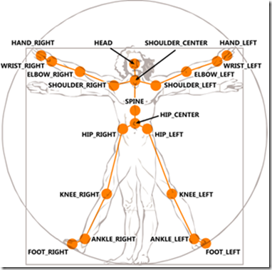
SC(t)=[angles(t),Stats(angles(t)),Calculus(angles(t))]

5.2.1 most active bone angles

let ”Origin” be tha Camera position as in [17].
Angle Category Joint 1 Vertex Joint 2 Right Shoulder Center Shoulder Right Elbow Right Arm Shoulder Right Elbow Right Wrist Right Angles Elbow Right Wrist Right Hand Right Left Shoulder Center Shoulder Left Elbow Left Arm Shoulder Left Elbow Left Wrist Left Angles Elbow Left Wrist Left Hand Left Right Hip Center Hip Right Knee Right Leg Hip Right Knee Right Ankle Right Angles Knee Right Ankle Right Foot Right Left Hip Center Hip Left Knee Left Leg Hip Left Knee Left Ankle Left Angles Knee Left Ankle Left Foot Left Symmetric Shoulder Left Shoulder Center Shoulder Right Angles Head Shoulder Center Spine Shoulder Center Spine Hip Center Big Elbow Left Shoulder Center Elbow Right Symmetric Wrist Left Shoulder Center Wrist Right Angles Knee Left Hip Center Knee Right Ankle Left Hip Center Ankle Right Big Wrist Left Hip Center Ankle Left Hand- Wrist Right Hip Center Ankle Right Foot Wrist Left Hip Center Ankle Right Angles Wrist Right Hip Center Ankle Left Wrist Left Origin Shoulder Center Elbow Left Origin Shoulder Center Shoulder Left Origin Shoulder Center Ankle Left Origin Hip Center Knee Left Origin Hip Center Camera- Hip Left Origin Hip Center Facing Wrist Right Origin Shoulder Center Angles Elbow Right Origin Shoulder Center Shoulder Right Origin Shoulder Center Ankle Right Origin Hip Center Knee Right Origin Hip Center Hip Right Origin Hip Center

\justify

5.3 Mixed-mode Stats-Calculus Pose Descriptor

It is formed from using similar features from both Cartesian Coordinates Stats-Calculus Pose descriptor and Angular Stats-Calculus Pose Descriptor.

Mixed(t)=[P(t),angles(P(t))]

SC(t)=[Mixed(t),Stats(Mixed(t)),Calculus(Mixed(t))]

5.4 Centro-Stats-Calculus Pose descriptor

For some moving actions as running, walking and some games as Fighting, It is needed to track position of the actor and his/her relative position during performing an action. So, no need to select a joint as origin for the system, but it is needed to define a dynamic positioned origin. our claim is using the centroid of all joints through all each action instance to be the origin for the system.

Centro(X,Y,Z)=\frac{\sum_{n=1}^{no.offrames}\sum_{j=1}^{no.ofjoints}Joint(j,n,X,Y,Z)}{no.offrames*no.ofjoints}

Same measures, performed on Cartesian Stats-Calculus descriptor, are used on $Centro(X,Y,Z)$ instead of $P(t)$ .

SC(t)=[Centro(X,Y,Z),Stats(Centro(X,Y,Z)),Calculus(Centro(X,Y,Z))]

5.5 Rela-Centro-Stats-Calculus Pose descriptor

For free moving actions, It is recommended to have a position tracker alongside a pose tracker, so a mix of Centro- and Cartesian Stats-Calculus is recommended for this case.

CentroSC(t)=[Centro(X,Y,Z),Stats(Centro(X,Y,Z)),Calculus(Centro(X,Y,Z))]

CartesianSC(t)=[P(t),Stats(P(t)),Calculus(P(t))]

SC(t)=[CentroSC(t),CartesianSC(t)]

5.6 Rela-Centro-Stats-Calculus DCT Pose descriptor

using transforms to uniquely differentiate between different poses is recommended.

•

calculate Discrete Cosine transform (DCT) of Rela-Centro-Stats-Calculus and truncating it to 100 dimension.

SC(t)=DCT([CentroSC(t),CartesianSC(t)])

5.7 Rela-Centro-Stats-Calculus DCT-AMDF Pose descriptor

using transforms to uniquely differentiate between different poses is recommended.

•

First, calculate Discrete Cosine transform of Rela-Centro-Stats-Calculus and truncating it to 100 dimension.
•

Second, calculating its average magnitude difference function (AMDF) at $N=45$ as in [1].

DCTSC(t)=DCT([CentroSC(t),CartesianSC(t)])

AMDF(t,k)=\frac{\sum_{n=1}^{N}{|DCTSC(t,n)-DCTSC(t,n+k)|}}{N}

6 Dimension Reduction

All Stats-Calculus Pose descriptor are normalized, in order to not bias to any component.
Due to high-dimensionality of features vector, so Principal Component Analysis is used to get efficient dimension reduction.

7 Vector Quantization

•

Affinity-Propagation [5] clustering algorithm is used to cluster similar pose descriptors, in order to use clusters identifiers as a representative to all its cluster pose descriptors during training and testing using Hidden Markov Model.

8 Training and testing Hidden Markov Model

•

Hidden Markov Model is trained using sequences of cluster labels of each frame descriptor for each performed action using Expectation-Maximization algorithm (so-called Baum-Welch) to maximize likelihood of sample learned features to get a Hidden Markov Model recognizer for each action.
•

Observations feed to Hidden Markov Model are sequences of clusters identifiers.
•

Viterbi (Dynamic Programming) algorithm is used to decode Hidden Markov Models system.

\justify

9 Recognition Experiments

This technique is tested on different data-sets:

•

UTKinect-Action Dataset [19, 3]
•

MSR-Action3D Dataset [18, 7]
•

MSR Daily Activity 3D Dataset [18]
•

Florence 3D actions Dataset [16, 4]

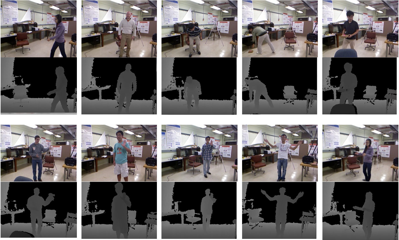
9.1 UTKinect-Action Dataset [19, 3]

”The videos was captured using a single stationary Kinect with Kinect for Windows SDK Beta Version. There are 10 action types: walk, sit down, stand up, pick up, carry, throw, push, pull, wave hands, clap hands. There are 10 subjects, Each subject performs each actions twice.”

9.1.1 3D Skeletal Action Recognition

* Experimental Setup: using subjects 1-5 for training and subjects 6-10 for testing.
descriptor accuracy HOJ3D [19] 90.92% Space-time Pose [3] 91.5% Centro-Stats-Calculus 68.8889% Rela-Centro-Stats-Calculus 80.0000% Rela-Centro-Stats-Calculus DCT-AMDF 97.7778%

9.2 MSR-Action3D Dataset [18, 7]

It consists of 20 actions performed 2-3 times by each of 10 subjects.
Some files are corrupted, according to [Wang et al. 18, Hussein et al. 7]
a02_s03_e02_skeleton3D, a04_s03_e01_skeleton3D,
a07_s04_e01_skeleton3D, a13_s09_e01_skeleton3D,
a13_s09_e02_skeleton3D, a13_s09_e03_skeleton3D,
a14_s03_e01_skeleton3D, a20_s07_e01_skeleton3D,
a20_s07_e03_skeleton3D and a20_s10_e03_skeleton3D

9.2.1 3D Skeletal Action Recognition

It is split into 3 overlapping action sets [ $AS1,AS2andAS3$ ], as in [6, 14, 8, 7, 3]
Two experimental setup are used

•

subjects 1,2,3,4,5 for training and 6,7,8,9,10 for testing as in [13]
descriptor Coordinates Stats-Calculus AS1 87.619% AS2 86.61% AS3 94.59% overall 89.6%
•

subjects 1,3,5,7,9 are used for training and 2,4,6,8,10 are used for testing as in [18, 8]
descriptor Coordinates Stats-Calculus Centro-Stats-Calculus Pose AS1 83.8095% 81.9048% AS2 86.6071% 85.7143% AS3 92.7928% 85.5856% overall 87.7365% 84.4015%

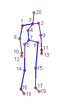
Figure 3: MSR-Action3D Dataset sample

method	accuracy
Recurrent Neural Network [18, 10, 20]	42.5%
Dynamic Temporal Warping [18, 12, 20]	54.0%
Hidden Markov Model [9, 20, 18]	63.0%
Latent-Dynamic CRF [11, 20]	64.8%
Latent-Dynamic Canonical Poses [20]	65.7%
Action Graph on Bag of 3D Points [18, 20]	74.7%
EigenJoints [20]	81.4%
Actionlet Ensemble [18]	88.2%
MP [20]	91.7%
Coordinates Stats-Calculus	89.6%

9.3 MSR Daily Activity 3D Dataset [18]

”The MSR Daily Activity 3D dataset is a most widely applied benchmark dataset in human behavior understanding tasks. This dataset contains 16 human activities, performed by 10 subjects. Each subject performs each activity twice, once in standing position and once in sitting position.”

9.3.1 3D Skeletal Action Recognition

method	accuracy
Dynamic Temporal Warping [12, 20]	54.0%
Actionlet Ensemble (3D pose only) [18, 20]	68.0%
MP [20]	73.8%
Rela-Centro-Stats-Calculus DCT-AMDF	87.5%

9.4 Florence 3D actions Dataset [16, 4]

”The dataset collected at the University of Florence during 2012, has been captured using a Kinect camera. It includes 9 activities: wave, drink from a bottle, answer phone,clap, tight lace, sit down, stand up, read watch, bow. During acquisition, 10 subjects were asked to perform the above actions for 2/3 times. This resulted in a total of 215 activity samples.”
* Experimental Setup: using 17 instance of each action for training and the remaining for testing

9.4.1 3D Skeletal Action Recognition

descriptor	accuracy
Bag-of-poses[16]	82%
Rela-Centro-Stats-Calculus DCT-AMDF	58.065%
Rela-Centro-Stats-Calculus DCT	68.8889%
Rela-Centro-Stats-Calculus	74.194%
Angular-Stats-Calculus	74.194%

3D Skeletal actions Detection using unsegemented sequences

adapted from the idea of segementation $-$ free OCR [15]

10 Methodology

Algorithm 2 Stats-Calculus HMM Detection

1:Bone Normalization

2:Features Extraction

3:Dimension Reduction

4:Vector Quantization

5:Training HMMs

6:Parallel Connections of HMMs

10.1 Dimension Reduction

10.2 Vector Quantization

•

Affinity-Propagation [5] clustering algorithm is used to cluster similar pose descriptors, in order to use clusters identifiers as a representative to all its cluster pose descriptors during training and testing using Hidden Markov Model.

10.3 Training and testing Hidden Markov Model (HMM)

•

Hidden Markov Model is trained using sequences of cluster labels of each frame descriptor for each performed action using Expectation-Maximization algorithm (so-called Baum-Welch) to maximize likelihood of sample learned features to get a Hidden Markov Model recognizer for each action.
•

Observations feed to Hidden Markov Model are sequences of clusters identifiers.
•

Viterbi (Dynamic Programming) algorithm is used to decode Hidden Markov Models system.

10.4 Parallel Connections of Hidden Markov Models (HMM)

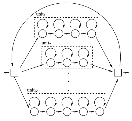
as in segmentation-free OCR [15] where each action previously trained Hidden Markov Model is a unit in the structure of a bigger Hidden Markov Model as showed in Figure 4

11 Detection Experiments using unsegemented sequences

This technique is tested on different data-sets:

•

UTKinect-Action Dataset [19, 3]
•

MSR-Action3D Dataset [18, 7]
•

Florence 3D actions Dataset [16, 4]

11.1 UTKinect-Action Dataset [19, 3]

* Experimental Setup: using subjects 1-3 for training and subjects 4-10 for testing.
* using a sliding-window of width = 7 frames, an Hidden MArkov Model (HMM) system of 3 states for each action. using Angular Stats-Calculus Pose Descriptor.
* Results:

precision=0.9984,recall=0.9753,F_{1}-Score=0.9867

11.2 MSR-Action3D Dataset

* Experimental Setup: using subjects 1-3 for training and subjects 4-10 for testing.
* using a sliding-window of width = 3 frames, an Hidden MArkov Model (HMM) system of 3 states for each action. using Angular Stats-Calculus Pose Descriptor.
* Results:

•

AS1:

precision=1.0,recall=1.0,F_{1}-Score=1.0

•

AS2:

precision=1.0,recall=0.9996,F_{1}-Score=0.9998

•

AS3:

precision=1.0,recall=0.9996,F_{1}-Score=0.9998

11.3 Florence 3D actions Dataset [16, 4]

* Experimental Setup: using instances 1-4 for training and instances 5-18 for testing.
* using a sliding-window of width = 3 frames, an Hidden MArkov Model (HMM) system of 3 states for each action. using Stats-Calculus Pose Descriptor.
* Results:

precision=1.0,recall=0.4210,F_{1}-Score=0.5926

12 Conclusion and Comparison

* A novel of Stats-Calculus Moving Pose descriptors framework is presented for both 3D skeletal action detection and recognition which uses pose, calculus kinematic information and statistical measures.

12.1 3D Skeleton actions Detection

method	Stats-Calculus	MP [20]
MSR-Action 3D [18, 7]	0.9998	0.892

13 Future Enhancement

* adding 2 extra angles for efficient Head-gestures as nodding

•

angle of: head—Shoulder Center—Shoulder Left.
•

angle of: head—Shoulder Center—Shoulder Right.

References

Apte [2012] Dr Shaila D Apte. Speech and audio processing, 2012.
Borse [1996] Garold J Borse. Numerical methods with MATLAB: A resource for scientists and engineers. International Thomson Publishing, 1996.
Devanne et al. [2013] Maxime Devanne, Hazem Wannous, Stefano Berretti, Pietro Pala, Mohamed Daoudi, and Alberto Del Bimbo. Space-time pose representation for 3d human action recognition. In New Trends in Image Analysis and Processing–ICIAP 2013, pages 456–464. Springer, 2013.
Devanne et al. [2014] Maxime Devanne, Hazem Wannous, Stefano Berretti, Pietro Pala, Meroua Daoudi, and Alberto Del Bimbo. 3-d human action recognition by shape analysis of motion trajectories on riemannian manifold. 2014.
Frey and Dueck [2007] Brendan J. Frey and Delbert Dueck. Clustering by passing messages between data points. Science, 315:972–976, 2007. URL www.psi.toronto.edu/affinitypropagation.
Gowayyed et al. [2013] Mohammad Gowayyed, Marwan Torki, Mohamed Hussein, and Motaz El-Saban. Histogram of oriented displacements (hod): Describing trajectories of human joints for action recognition. In International Joint Conference on Artificial Intelligence (IJCAI), Beijing, China, August 2013.
Hussein et al. [2013] Mohamed Hussein, Marwan Torki, Mohammad Gowayyed, and Motaz El-Saban. Human action recognition using a temporal hierarchy of covariance descriptors on 3d joint locations. In International Joint Conference on Artificial Intelligence (IJCAI), Beijing, China, August 2013.
Li et al. [2010] Wanqing Li, Zhengyou Zhang, and Zicheng Liu. Action recognition based on a bag of 3d points. In Computer Vision and Pattern Recognition Workshops (CVPRW), 2010 IEEE Computer Society Conference on, pages 9–14. IEEE, 2010.
Lv and Nevatia [2006] Fengjun Lv and Ramakant Nevatia. Recognition and segmentation of 3-d human action using hmm and multi-class adaboost. In Computer Vision–ECCV 2006, pages 359–372. Springer, 2006.
Martens and Sutskever [2011] James Martens and Ilya Sutskever. Learning recurrent neural networks with hessian-free optimization. In Proceedings of the 28th International Conference on Machine Learning (ICML-11), pages 1033–1040, 2011.
Morency et al. [2007] Louis-Philippe Morency, Ariadna Quattoni, and Trevor Darrell. Latent-dynamic discriminative models for continuous gesture recognition. In Computer Vision and Pattern Recognition, 2007. CVPR’07. IEEE Conference on, pages 1–8. IEEE, 2007.
Müller and Röder [2006] Meinard Müller and Tido Röder. Motion templates for automatic classification and retrieval of motion capture data. In Proceedings of the 2006 ACM SIGGRAPH/Eurographics symposium on Computer animation, pages 137–146. Eurographics Association, 2006.
Oreifej and Liu [2013] Omar Oreifej and Zicheng Liu. Hon4d: Histogram of oriented 4d normals for activity recognition from depth sequences. In Computer Vision and Pattern Recognition (CVPR), 2013 IEEE Conference on, pages 716–723. IEEE, 2013.
Padilla-López et al. [2014] José Ramón Padilla-López, Alexandros André Chaaraoui, and Francisco Flórez-Revuelta. A discussion on the validation tests employed to compare human action recognition methods using the msr action3d dataset. arXiv preprint arXiv:1407.7390, 2014.
Plötz and Fink [2009] Thomas Plötz and Gernot A Fink. Markov models for offline handwriting recognition: a survey. International Journal on Document Analysis and Recognition (IJDAR), 12(4):269–298, 2009.
Seidenari et al. [2013] Lorenzo Seidenari, Vincenzo Varano, Stefano Berretti, Alberto Del Bimbo, and Pietro Pala. Recognizing actions from depth cameras as weakly aligned multi-part bag-of-poses. In Computer Vision and Pattern Recognition Workshops (CVPRW), 2013 IEEE Conference on, pages 479–485. IEEE, 2013.
Sharaf et al. [2015] Amr Sharaf, Marwan Torki, Mohamed E. Hussein, and Motaz El-Saban. Real-time multi-scale action detection from 3d skeleton data. In IEEE Winter Conference on Applications of Computer Vision (WACV), Waikoloa Beach, HI, January 2015.
Wang et al. [2012] Jiang Wang, Zicheng Liu, Ying Wu, and Junsong Yuan. Mining actionlet ensemble for action recognition with depth cameras. In Computer Vision and Pattern Recognition (CVPR), 2012 IEEE Conference on, pages 1290–1297. IEEE, 2012.
Xia et al. [2012] L. Xia, C.C. Chen, and JK Aggarwal. View invariant human action recognition using histograms of 3d joints. In Computer Vision and Pattern Recognition Workshops (CVPRW), 2012 IEEE Computer Society Conference on, pages 20–27. IEEE, 2012.
Zanfir et al. [2013] Mihai Zanfir, Marius Leordeanu, and Cristian Sminchisescu. The moving pose: An efficient 3d kinematics descriptor for low-latency action recognition and detection. 2013.

Author

Rofael Emil Fayez Behnam

Computer and Systems Engineering

Faculty of Engineering

Alexandria University- Egypt

rofaelemil@gmail.com

Bachelor of Computer and Systems Engineering, $4^{th}$ year, Computer and Systems Engineering department, Faculty of Engineering, Alexandria University [2011- 2016]

expected July 2016 (86.8% $-$ Distinction)