The NANOGrav Nine-year Data Set: Astrometric Measurements of 37 Millisecond Pulsars

Abstract

Using the nine-year radio-pulsar timing data set from the North American Nanohertz Observatory for Gravitational Waves (NANOGrav), collected at Arecibo Observatory and the Green Bank Telescope, we have measured the positions, proper motions, and parallaxes for 37 millisecond pulsars. We report twelve significant parallax measurements and distance measurements, and eighteen lower limits on distance. We compare these measurements to distances predicted by the NE2001 interstellar electron density model and find them to be in general agreement. We use measured orbital-decay rates and spin-down rates to confirm two of the parallax distances and to place distance upper limits on other sources; these distance limits agree with the parallax distances with one exception, PSR J1024$-$0719, which we discuss at length. Using the proper motions of the 37 NANOGrav pulsars in combination with other published measurements, we calculate the velocity dispersion of the millisecond pulsar population in Galactocentric coordinates. We find the radial, azimuthal, and perpendicular dispersions to be $46$, $40$, and $24$ km s^-1, respectively, in a model that allows for high-velocity outliers; or $81$, $58$, and $62$ km s^-1 for the full population. These velocity dispersions are far smaller than those of the canonical pulsar population, and are similar to older Galactic disk populations. This suggests that millisecond pulsar velocities are largely attributable to their being an old population rather than being artifacts of their birth and evolution as neutron star binary systems. The components of these velocity dispersions follow similar proportions to other Galactic populations, suggesting that our results are not biased by selection effects.

1. Introduction

Distance and velocity measurements of millisecond pulsars can be used to constrain models of supernova dynamics, binary star evolution, pulsar emission physics, and the ionized interstellar medium. They can characterize the millisecond pulsar population as a whole, and they can be used to probe the kinematic evolution of the millisecond pulsar population in the Galaxy and its relation to other stellar populations.

Pulsar timing allows for high precision measurement of millisecond pulsar positions, parallaxes, and proper motions. Pulse times of arrival (TOAs) measured over the course of a year vary in part due to the changing time-of-flight of the pulses across the solar system, i.e., the Roemer delay. This variation is approximately sinusoidal with a period of one year. The phase and amplitude of this pattern can be used to infer the ecliptic longitude and latitude of the pulsar, respectively. For many millisecond pulsars, TOAs can be measured to a precision well under a microsecond, yielding position measurements with precision of order milliarcseconds or better. Measurements of positions over several years can be used to infer proper motions with precision of milliarcseconds per year. Such highly precise TOA measurements can also be used to infer pulsar parallaxes, and hence distances, out to distances of order a kiloparsec. Proper motions and distances combine to yield two components of the pulsar velocity vectors.

Canonical (non-millisecond) pulsars are well known to be high velocity objects. For example, the proper motion study of Hobbs et al. (2005) found that canonical pulsars have mean speeds of $152\pm 10$ km s^-1when measured in one dimension and $246\pm 22$ km/s when measured in two dimensions; from this they inferred that pulsars are formed in a thin disk with a mean birth speed of $400\pm 40$ km/s. These high velocities presumably result from asymmetries in supernova explosions, possibly combined with pre-supernova orbital and space motion of the pulsar progenitor.

In contrast, early studies of millisecond pulsars showed their space velocities to be much lower than those of canonical pulsars (Nice & Taylor, 1995; Cordes & Chernoff, 1997). This has been confirmed by, among others, Hobbs et al. (2005), whose analysis of recycled pulsars (which they defined as having spin periods $P<100$ ms and spin-down rates $\dot{P}<10^{-17}$) found their one-dimensional and two-dimensional mean speeds to be $54\pm 6$ km s^-1and $87\pm 13$ km s^-1, respectively. Gonzalez et al. (2011), whose analysis of millisecond pulsars (which they defined to have spin periods $P<10$ ms) found their mean two-dimensional speed to be $108\pm 15$ km/s.

The relatively small space velocities of millisecond pulsars are likely a byproduct of their formation process. According to the conventional scenario, a millisecond pulsar is formed as a canonical pulsar and then spun-up to its millisecond rotational period via mass accretion from a binary companion, (Alpar et al., 1982). If a neutron star in a binary system is formed with a large kick, the binary is likely to be disrupted, and the binary accretion needed to form a millisecond pulsar cannot take place. Only binary systems with small or fortuitously oriented kicks survive and allow formation of millisecond pulsars. Alternatively, low-velocity kicks may result from electron-capture supernovae, and the millisecond pulsars may be formed via accretion-induced collapse of a white dwarf during mass transfer in a binary (e.g., van den Heuvel, 2011; Freire & Tauris, 2014).

One might expect correlations between millisecond pulsar kinematics and orbital properties, i.e., different velocity distributions for isolated and binary millisecond pulsars; and, among binary millisecond pulsars, a dependence of velocity on orbital period or mass function (e.g., Tauris & Bailes, 1996). Indeed, Ng et al. (2014) found greater Galactic heights for lower-mass binary millisecond pulsar systems. Lommen et al. (2006) compared isolated and binary millisecond pulsars and found that they had indistinguishable velocity distributions, but that observed binary pulsars had a larger Galactic scale height, leading to speculation that the two populations have different luminosity distributions, with isolated pulsars weaker and therefore more difficult to detect at large distances; however, Lorimer et al. (2007) argue that this could arise from selection effects in pulsar searches. Gonzalez et al. (2011), analyzing a larger sample of millisecond pulsars, also found the velocity distributions of binary and isolated millisecond pulsars to be indistinguishable.

Stellar populations in the solar neighborhood have ellipsoidal velocity distributions. Cordes & Chernoff (1997) show that analysis of these velocity distributions can give insight into the dynamical history of millisecond pulsars, including both the magnitudes of any kicks received at formation and the diffusion of these pulsars through the Galaxy. We adopt Galactocentric coordinates, with $v_{R}$, $v_{\phi}$, and $v_{z}$ in the direction of the Galactic center, the direction of Galactic rotation, and the direction perpendicular to the Galactic disk, respectively, and we denote their velocity dispersions by $\sigma_{R}$, $\sigma_{\phi}$, and $\sigma_{z}$. It is well established theoretically and observationally that, for any given stellar population, $\sigma_{R}>\sigma_{\phi}>\sigma_{z}$, with typical ratios $\sigma_{z}/\sigma_{R}\simeq 0.5$ and $\sigma_{\phi}/\sigma_{R}\simeq 0.55\ {\rm to}\ 0.7$ (Binney & Merrifield, 1998, §10.3.2; for simplicity, we ignore vertex deviation). Analyzing millisecond pulsar velocities in Galactocentric coordinates has three advantages. (i) It facilitates comparisons with other stellar populations. (ii) The consistency of the magnitudes of the different components can be used to cross-check the measured velocity distributions. (iii) If a component were biased by selection effects—in particular, pulsar searches are preferentially made along the Galactic plane, and one could imagine this biasing the distribution of $v_{z}$—the other components might still give unbiased results.

The NANOGrav collaboration is undertaking long-term timing of several dozen millisecond pulsars for the purpose of detecting and characterizing gravitational waves via their perturbation of millisecond pulsar TOAs on time scales of tens of years (frequencies of nanohertz). The detection of gravitational wave signals requires the modeling and removal of all other phenomena that influence pulse arrival times, including solar system time-of-flight effects which yield the astrometric measurements described above. The NANOGrav nine-year data release (Arzoumanian et al., 2015) reports timing observations of 37 pulsars collected over nine years, and includes pulse timing models for all of these pulsars. In the present paper, we analyze the astrometric parameters from that work.

In § 2, we summarize the observations. In § 3, we list the parameters resulting from the timing analysis. In § 4, we discuss the distances inferred from the timing measurements. In § 5, we combine our newly measured millisecond pulsar velocities with previous measurements to analyze the kinematics of the millisecond pulsar population as a whole. In § 6, we summarize our results.

Except where otherwise specified, we define a millisecond pulsar to be a pulsar with rotational period of 20 ms or less, and a spin-down rate of less than $10^{-17}\,{\rm s}\,{\rm s}^{-1}$, a definition that includes all pulsars observed in the NANOGrav program. We exclude pulsars in globular clusters from our study, because no NANOGrav sources are in globular clusters, and because the formation and dynamics of millisecond pulsars in globular clusters are different than those of millisecond pulsars in the Galactic disk.

2. Observations

2.1. Overview of the NANOGrav nine-year data set

We use data from the NANOGrav nine-year data set, which we briefly summarize here. For full details see Arzoumanian et al. (2015). Observations of 37 millisecond pulsars were made using the Arecibo Observatory (AO) and the Green Bank Telescope (GBT). The project began with 15 pulsars in 2004, and new pulsars were added to the project as they were discovered or when wide-band data acquisition systems enabled sources previously deemed unreliable to be precisely timed. Pulsars were chosen based on high timing precision, detectability over a wide frequency range, and expected timing stability. The nine-year data set includes observations through 2013. Observed time spans of individual pulsars range from 0.6 yr to 9.2 yr.

Each pulsar was observed at approximately monthly intervals. At every epoch, each pulsar was observed for approximately $25$ minutes each using two different radio telescope receivers at widely separated frequencies. Such dual-receiver observations allow for measurement and removal of interstellar and solar-system dispersive effects. (In a small number of cases, dual-receiver observations were not available, but single-receiver observations were made over a wide observing band.)

Observations in early years of the project used the Astronomical Signal Processor (ASP) at AO and the Green Bank Astronomical Signal Processor (GASP) at the GBT; each sampled up to 64 MHz bandwidth, depending on telescope receiver capability. In the later years, observations used the Puerto Rican Ultimate Pulsar Processor (PUPPI) at AO and the Green Bank Ultimate Pulsar Processor (GUPPI) at the GBT; each provided up to 800 MHz bandwidth, again depending on telescope receiver capability.

The data were polarization-calibrated, cleaned of radio frequency interference, and analyzed to produce TOAs using a standardized pipeline that made extensive use of the psrchive software package (van Straten et al., 2012). The sets of TOAs were fit to timing models using the tempo and tempo2 packages. We found that these packages yielded essentially identical results, and we used tempo for the work in the present paper .

The timing models contain standard spin-down, astrometric, and (where appropriate) binary models. The astrometric parameter measurements are the basis for the present paper and are described in more detail in §3. Criteria for inclusion of specific parameters in the timing model for each pulsar are given in Arzoumanian et al. (2015).

In the timing analysis, Earth motion around the solar-system barycenter was modeled using the JPL DE421 planetary ephemeris (Folkner et al., 2009). TOAs were measured using hydrogen-maser clocks at the observatories and were transformed to Universal Time and then to Barycentric Dynamical Time using standard techniques.

Separate values of dispersion measure were fit independently at every observing epoch, with a few exceptions (see Arzoumanian et al. (2015) for details). This results in timing parameter uncertainties that are larger than would be found using smoothed dispersion measure models, but is necessary to avoid contamination of our results by variations in interstellar and solar wind dispersion. The latter, in particular, is not easily modeled, and is highly covariant with the astrometric parameters of interest to this paper.

A novel noise model was used to account for any aspects of the timing data that did not fit the standard timing model within the expected measurement uncertainties. The noise model incorporated white noise, correlated noise in simultaneously collected TOAs, and red noise (as needed for a few sources). Details are given in Arzoumanian et al. (2015).

The full data set, including TOAs and timing parameters of all pulsars, is available online.

2.2. Data set modifications for this work

We made a small number of modifications to the NANOGrav nine-year data set for the present work.

The data sets of PSRs J1741+1351, J1853+1303, J1910+1256, J1944+0907, and B1953+29 contain lengthy spans in which observations were made using only a single, narrow-band receiver, eliminating the possibility of monitoring and correcting for dispersion measure variation over those spans. We excised the TOA measurements from those data spans. We re-evaluated the timing models for these pulsars using the remaining TOAs, following the same guidelines used by Arzoumanian et al. (2015) for noise models, parameter inclusion, etc.

The timing solution for PSR J2317+1439 in the NANOGrav nine-year data release included secular variations of the Laplace-Lagrange orbital elements, which are formally significant in the fit, but which are physically implausible. We removed those parameters from the timing solution. We then re-evaluated the timing model using the guidelines of Arzoumanian et al. (2015), following which we added Shapiro delay parameters (now significant) and eliminated the secular variation in the projected orbital semi-major axis (now not significant). Details of the analysis of this and other binaries will be given in a forthcoming paper (Fonseca et al., in preparation).

The modified timing solutions used for this paper are bundled with the NANOGrav nine-year data release files.

3. Measured astrometric parameters

3.1. Positions

The timing analysis of the NANOGrav nine-year data set parameterizes pulsar positions in ecliptic coordinates. These are natural coordinates for pulsar timing astrometry, as ecliptic longitude and latitude are nearly orthogonal parameters in the timing fit. Table 1 lists the ecliptic and equatorial positions of all of the pulsars in the data set. The epoch of each position was chosen near the middle of its data set in order to minimize covariance between position and proper motion parameters. The reference frame for these position measurements is the reference frame of JPL planetary ephemeris DE421, which is oriented to the International Celestial Reference Frame (Folkner et al., 2009). The ephemeris coordinates were transformed into ecliptic coordinates by a rotation of $23^{\circ}26\arcmin 21\farcs 406$, the IERS2010 obliquity of the ecliptic.

For observational convenience, Table 1 also lists the positions in equatorial coordinates. The equatorial positions were determined by fitting timing solutions without rotating the planetary ephemeris into ecliptic coordinates. As shown in Figure 1, uncertainties in equatorial coordinates are generally larger than uncertainties in ecliptic coordinates. This is particularly true when one ecliptic coordinate is measured much more precisely than the other (e.g., for pulsars along the ecliptic).

3.2. Proper Motions

Proper motion, $\mu_{\alpha}=\dot{\alpha}~{}{\rm cos}\delta$ and $\mu_{\delta}=\dot{\delta}$, was included in the timing model for 35 of the 37 pulsars in our data set. The two pulsars for which proper motion was excluded have less than one year of timing measurements in our data set, making it impossible to measure their proper motions. Lengths of all of the data sets are given in Table 2.

The proper motions from timing analyses in both ecliptic and equatorial coordinates are listed in Table 2. As with the position measurements, ecliptic coordinates provide the best separation of proper motion into orthogonal components, and hence the smallest uncertainties. The table also includes proper motions in Galactic coordinates.

The best previous proper motion measurements in ecliptic coordinates are listed in Table 2. All the new and previous measurements agree to within $3\sigma$ except for two pulsars (PSRs J1909$-$3744 and J2145$-$0750) which have discrepancies between $3\sigma$ and $4\sigma$ for at least one component of proper motion. The proper motions of these two pulsars are known to high precision, and these small discrepancies have little practical impact. We speculate that the differences may be due to differences in dispersion measure variation models (as we discuss for parallax measurements in § 3.3.1), or differences in solar system ephemerides used in the timing analysis.

Our measured proper motions are illustrated in Figure 2. We discuss the derivation of two- and three-dimensional space velocities from these proper motions in § 5.

3.3. Parallaxes

We included parallax, $\varpi$, as a free parameter in the timing model for each pulsar, whether or not the measurement was statistically significant. The timing analysis allowed both negative and positive parallaxes. Although negative parallaxes are non-physical, allowing them in the timing solutions provides a useful a check on the reliability of the measurements (§3.3.2). The measured parallax values are listed in Table 3 and shown in Figure 3. Previous measurements for these pulsars are also included in the Table and Figure.

There were no previously reported parallax measurements or limits for 20 of the 37 pulsars. Of these 20 sources, two provided significant new parallax measurements: PSR J1918$-$0642, $\varpi=1.1\pm 0.2$ mas; and PSR J2043+1711, $\varpi=0.8\pm 0.2$ mas.

3.3.1 Comparison with previous measurements

Of the 17 pulsars with previous measurements or limits, we improved the precision of four measurements by a factor of two or better: PSRs J0030+0451, J0613$-$0200, J1600$-$3053, and J1614$-$2230.

For PSR J1713+0747, in addition to the previous timing parallax value of 0.94(5) given in Table 3, there are two other previous measurements of interest. One is from an analysis of 21 years of data from this pulsar by Zhu et al. (2015), which obtained a parallax of $\varpi=0.85\pm 0.03$ mas, identical to our own measurement. This is not surprising, as the vast majority of the TOAs in the Zhu et al. (2015) analysis were from the same NANOGrav nine-year data set that is being used for the present work. The other previous parallax measurement of J 1713+0747 is from the interferometric VLBA measurements of Chatterjee et al. (2009), which obtained $\varpi=0.95\pm 0.06$ mas, in reasonable agreement ($1.5\sigma$) with our value.

In most other cases, our parallax values also agree with previous measurements. However, there are discrepancies of 2$\sigma$ or more (i.e., disagreement at 95% confidence) between our measurements and the previous measurements for three sources: PSRs J1643$-$1224, B1855+09, and J1909$-$3744. A possible explanation for these discrepancies is the difference in treatment of dispersion measure (DM) variations. Small variations in the ionized component of the interstellar medium and the solar wind along the pulsar–Earth line-of-sight significantly affect TOAs. To minimize contamination of the timing analysis from DM variations on the half-yearly time scale of the parallax signal (as well as other time scales of interest to pulsar modeling), we fit for DM at every epoch of observation. Since the DM variations are covariant with the parallax signal in the timing fit, this increases formal uncertainties on our parallax measurements, but it also makes the measurements more robust.

The previous parallax analysis of two of the discrepant sources—PSRs J1643$-$1224, and B1855+09—assumed a constant value of DM over the entire data set (see references in Table 3). The third, PSR J1909$-$3744 (Verbiest et al., 2009), used the smoothed DM time series model of You et al. (2007), which includes a smoothing time scale longer than the half-year period of the parallax signature in the timing model. To test the effect of using constant or smoothed DM variation models, we ran trials of timing analyses of these sources fitting (i) a constant DM and (ii) a model of DM as a up-to-fifth-order polynomial in time over the entire data sets. These tests yielded changes in measured parallax values by amounts ranging from $0.2\sigma$ to $10\sigma$, with three of the four values moving by at least $1\sigma$. We therefore believe that limited DM variation modeling is a plausible explanation for the discrepancies between previously measured parallax values and our measurements.

3.3.2 Measurements with low significance

The timing analyses of a majority of the pulsars we analyzed did not yield significant parallax detections. To illustrate the nature of these non-detections, we sorted the pulsars by parallax measurement significance, $\varpi/\sigma_{\varpi}$, and plotted the cumulative distribution of these values in Figure 4. Of the 37 parallax measurements, 12 are significant positive detections of parallax, $\varpi/\sigma_{\varpi}>3$. No sources had significant negative detections of parallax, $\varpi/\sigma_{\varpi}<-3$. (Although negative parallax values are unphysical, corresponding to pulse wavefronts with concave rather than convex curvature relative to the pulsar, they were allowed in the timing analysis. A significant negative parallax measurement would indicate a problem with the data or the timing model.) Of the 25 pulsars with non-detections, only 7 measurements are negative, all but two within $1\sigma$ of zero, and the remaining 18 are positive. This bias toward positive values indicates that most of these are indeed real, physical measurements, and significant parallax values should be attainable for many of them with only moderately larger data sets.

4. Distances

4.1. Distances from parallax measurements

We now use the parallaxes in Table 3 to analyze distances to 30 of the 37 pulsars. The timing data sets of the other 7 pulsars span less than 2 years, which is typically not sufficient time to disentangle position, proper motion, and parallax in the timing analysis. Indeed, none of these sources had nominally significant parallax measurements, and 3 of them had negative parallaxes.

For the 12 pulsars with significant parallax measurements, $\varpi/\sigma_{\varpi}>3$, we calculated distances as listed in the upper portion of Table 4. For each of these pulsars, the central distance value, upper limit, and lower limit given in the table were calculated using $d=\varpi^{-1}$, where $\varpi$ was the 84%, 50%, and 16% points in the measured parallax distribution, respectively, corresponding to the 16%, 50% and 84% points in the distance distribution.

For the 18 remaining pulsars, we used 95% confidence upper limits on parallax to compute 95% confidence lower limits on distance. To find the upper limits on parallax, we first verified that changes in assumed parallax values in the timing solution yielded changes in goodness-of-fit $\chi^{2}$ values appropriate for parallax values drawn from a Gaussian distribution. We then found the 95% confidence upper limits on $\varpi$ by calculating the value of $\varpi$ at which 95% of the area under the Gaussian distribution of the parallax was at lower values, but restricting the integral to positive values of parallax. The resulting parallax limits are listed in Table 4. The corresponding $95\%$ confidence lower limit on distance for each source was then calculated to be the reciprocal of this value. These are also listed in Table 4.

The Lutz-Kelker bias (Lutz & Kelker, 1973) may be significant for the distance measurements of pulsars with large uncertainties on parallax. The bias can be incorporated as a correction to parallax and distance values through methods outlined by Verbiest et al. (2010) and Verbiest et al. (2012). The Bayesian analysis used under these methods assumes a uniform prior distribution of a pulsar’s position throughout three-dimensional space. Since there is more three-dimensional space at larger distances than at smaller distances, this has the effect of moving the posterior distribution of a pulsar’s distance to values larger than that calculated from $d=\varpi^{-1}$. This is problematic for pulsars for which there are only upper limits on parallax, as this allows a finite probability of $\varpi_{\rm measured}=0$, which corresponds to infinitely large distances, at which there is infinite parameter space. To achieve a tractable result, some additional prior must be invoked to cut off the likelihood of the pulsar being at a large distance. One possibility is to use a model of the Galactic distribution of millisecond pulsars, but we want our results to stand independent of a priori beliefs about the Galactic distribution of millisecond pulsars; further, we found that attempts to use prior Galactic distribution models tended to give results that were dominated by the details of the model. Another possibility is to model the sensitivity of pulsar search programs, which find nearby pulsars more readily than distant pulsars; however, we found that use of such a prior gave results that were highly dependent on the choice of millisecond pulsar luminosity distribution, which is not well known.

For these reasons, we elected not to apply any corrections to the distances in Table 4. For sources for which we give lower limits on distances (lower portion of Table 4), this is a conservative approach from a Lutz-Kelker perspective, in the sense that the Lutz-Kelker bias would place these pulsars still further than our lower-limit distances. For the twelve sources for which we give distance measurements (upper portion of Table 4), we tested the effect of Lutz-Kelker corrections by running the measurements through the Lutz-Kelker bias code from Verbiest et al. (2012). We found the differences in calculated distances to be small; for example, six of the central distance measurement values were unchanged, and the other six all changed by less than $1\sigma$ (typically much less).

4.2. Distances from orbital period derivatives

In addition to timing parallax, there are other means by which distances can be inferred from pulsar timing. One such approach uses the observed properties of binary pulsars. The observed orbital period, $P_{\rm b}$, of a binary pulsar undergoes a time change $\dot{P}_{\rm b}$ due to mass loss from the system (negligible here), general relativistic phenomena, and kinematic effects (Damour & Taylor, 1991),

$$\left(\frac{\dot{P}_{\rm b}}{{P}_{\rm b}}\right)_{\rm obs}=\left(\frac{\dot{P}_{\rm b}}{{P}_{\rm b}}\right)_{\rm GR}+\left(\frac{\dot{P}_{\rm b}}{{P}_{\rm b}}\right)_{\rm kin}.$$ (1)

The relativistic term, $\left(\dot{P}_{b}/P_{b}\right)_{\rm GR}$, is the orbital decay due to emission of gravitational radiation, which depends on the component masses and other orbital elements. The kinematic term, $\left(\dot{P}_{b}/P_{b}\right)_{\rm kin}$, is due to the relative acceleration of the binary system and the Sun, which causes changes in the Doppler shift of the observed period. The relevant expression from Damour & Taylor (1991), here modified to apply to pulsars off the Galactic plane (Nice & Taylor, 1995), is

$$\left(\frac{\dot{P}_{\rm b}}{{P}_{\rm b}}\right)_{\rm kin}=\frac{a_{z}(z)}{c}-\cos b\left(\frac{\Theta_{0}^{2}}{cR_{0}}\right)\left(\cos l+\frac{\beta}{\sin^{2}l+\beta^{2}}\right)+\frac{\mu^{2}d}{c},$$ (2)

where the terms on the right hand side are as follows. The first term is the acceleration of the binary system in the Galactic potential perpendicular to the disk, $a_{z}$, which depends on the perpendicular distance $z=d\sin b$ , where $b$ is the Galactic latitude, and $c$ is the speed of light. The second term is the line-of-sight acceleration due to differential rotation in the Galaxy; here $R_{0}$ is the Galactocentric distance of the solar system; $\Theta_{0}$ is the circular rotation speed of the Galaxy at $R_{0}$; $l$ is the Galactic longitude; and $\beta=(d/R_{0})\cos b-\cos l$. The third term is the apparent acceleration due to proper motion (Shklovskii, 1970). Each of these terms depends on the distance to the pulsar; as Bell & Bailes (1996) pointed out, given a measurement $(\dot{P}_{\rm b}/{P}_{\rm b})_{\rm obs}$ and a calculated $(\dot{P}_{\rm b}/{P}_{\rm b})_{\rm GR}$, one can solve equations 1 and  2 to infer the distance to the pulsar. This method has been used to compute high-precision distances to PSRs J0437-4715 (Verbiest et al., 2008) and B1534+12 (Fonseca et al., 2014). In cases where the measurement of $\dot{P}_{\rm b}$ is marginal or not significant, this method can be used to place an upper limit on the pulsar distance.

There are 25 binary pulsars in the NANOGrav nine-year data set. A full analysis of these systems will be presented in Fonseca et al. (in preparation). For the present work, we considered 22 of these pulsars which have been observed for at least two years. For each of these, we (i) fit for $\dot{P}_{\rm b}$ in the timing solution of the pulsar, (ii) calculated the expected $\dot{P}_{\rm b}$ as a function of distance according to equations 1 and 2, (iii) compared the calculated $\dot{P}_{\rm b}$ values with the measured value and its uncertainty to find a probability associated with that distance, and (iv) used the probabilities to calculate either the distance and its uncertainty or a 95% upper limit on the distance. For the $\dot{P}_{\rm b}$ calculations, the GR term is negligible for wide binary systems; for tight binaries, we estimated $(\dot{P}_{\rm b})_{\rm GR}$ using masses from analysis of the Shapiro delay in each system (Fonseca et al., in prep), except for the case of PSR J1012+5307, where we used masses derived from the optical measurements of Callanan et al. (1998). For the acceleration toward the Galactic disk, $a_{z}(z)$, we used the model of the Galactic potential given in equation 17 of Lazaridis et al. (2009), based on the Galactic potential of Holmberg & Flynn (2004); other Galactic potential models, such as that of Kuijken & Gilmore (1989), give essentially identical results. We used $R_{0}=8.34$ kpc and $\Theta_{0}$=240 km s^-1 (Reid et al., 2014). For the proper motion term in the $\dot{P}_{\rm b}$ calculations, we used the proper motions given in Table 2.

We found that 15 of the 22 pulsars had distance upper limits greater than 15 kpc. Since such limits are of little interest, and since this is beyond any reasonable extrapolation of the Galactic rotation and acceleration models, we did not analyze these further. Of the seven remaining pulsars, we measured significant distance constraints (at least $2\sigma$) for two sources, and we placed distance upper limits on the other five sources ($d_{\dot{P}_{b}}$ in Table 5.) In all cases, these measurements are consistent with the distance measurements or limits we found via parallax measurement (Table 4).

The most precise $\dot{P}_{\rm b}$ distance measurement is that of PSR J1909$-$3744, $1.11\pm 0.02$ kpc. This is a good match for our parallax distance of $1.07\pm 0.03$ kpc. The best previous parallax measurement, $\varpi=0.79\pm 0.04$ mas ($2\sigma$, Verbiest et al., 2009) gave a somewhat larger distance of $1.26\pm 0.03$ kpc ($1\sigma$, Verbiest et al., 2012). As discussed above, we suggest the difference between previous and presently measured parallaxes may result from differences in the dispersion measure model used in the timing analysis. The distance derived from $\dot{P}_{\rm b}$ is relatively impervious to changes in the dispersion measure model, so it provides a good verification of our parallax distance measurement.

Finally, we note that $\dot{P}_{\rm b}$ values of two sources, PSRs J1012+5307 and J1713+0747, have been measured more precisely than in the present paper (Lazaridis et al., 2009; Zhu et al., 2015). Those works focused on the use of $\dot{P}_{\rm b}$ measurements to test relativistic gravity rather than measuring distances. Using those $\dot{P}_{\rm b}$ measurements in our distance algorithms above gives distance upper limits of $d<4.8$ kpc and $d<17$ kpc, for PSRs J1012+5307 and J1713+0747, respectively. These constraints, while weak, are consistent with our parallax distance measurements and limits.

4.3. Distance constraints from rotation period derivatives

Another set of constraints on pulsar distances arises from their spin-down rates (Nice & Taylor, 1995). A variant on equation 1 can be applied to a pulsar rotation period, $P$, and spin-down rate, $\dot{P}$. The observed spin-down rate, $\dot{P}_{\rm obs}$ depends on both the intrinsic spin-down rate, $\dot{P}_{\rm int}$, and kinematic corrections:

$$\left(\frac{\dot{P}}{P}\right)_{\rm obs}=\left(\frac{\dot{P}}{P}\right)_{\rm int}+\left(\frac{\dot{P}}{P}\right)_{\rm kin}.$$ (3)

The kinematic term, $(\dot{P}/P)_{\rm kin}$, obeys the same expression as equation 2, substituting rotational for orbital parameters,

$$\left(\frac{\dot{P}}{P}\right)_{\rm kin}=\frac{a_{z}(z)}{c}-\cos b\left(\frac{\Theta_{0}^{2}}{cR_{0}}\right)\left(\cos l+\frac{\beta}{\sin^{2}l+\beta^{2}}\right)+\frac{\mu^{2}d}{c}.$$ (4)

If we presume that millisecond pulsars are powered by rotational energy loss, then $(\dot{P}/P)_{\rm int}>0$. From this, equation 3 implies $(\dot{P}/P)_{\rm kin}<(\dot{P}/P)_{\rm obs}$, so the observed spin parameters place an upper limit on this kinematic term. The right hand side of equation 4 is generally a monotonically increasing function of distance, so the upper limit on $(\dot{P}/P)_{\rm kin}$ sets an upper limit on distance.

We used equations 3 and 4 to place upper limits on distances to the 30 pulsars in the NANOGrav nine-year data set that have been observed for at least 2 years, so that they have well-measured proper motions. We used the Galactic rotation and acceleration parameters described in §4.2. We found that 12 of these pulsars had distance limits greater than 15 kpc; we did not pursue these further. The spin-down distance limits, $d_{\dot{P}}$, of the remaining 17 pulsars are listed in Table 6.

Most of the spin-down distance constraints agree with the distances derived from parallax measurements. Indeed, all of the parallax distances measured with at least 3$\sigma$ precision (Table 4) fall within the spin-down distance limit constraints (Table 6). The pulsar for which the spin-down distance limit comes closest to the parallax distance is PSR J1909$-3744$, for which the spin-down limit is $d_{\dot{P}}<1.375$ kpc and the parallax distance is $d_{\varpi}=1.07\pm 0.03$ kpc, providing a good check on the parallax distance.

For the pulsars for which we have only an upper limit on parallax, and therefore a lower limit on distance (Table 4), all but one are in agreement with the spin-down distance limits. In these cases, the pair of distance constraints bracket the actual distance to the pulsar.

For PSR J1024$-$0719, the spin-down distance upper limit, $d_{\dot{P}}<0.427$ kpc, disagrees with the parallax distance lower limit, $d_{\varpi}>0.91$ kpc. This is perplexing. The spin-down distance limit should be robust, presuming that the pulsar is losing energy and not subject to external acceleration. We have run several tests on our parallax measurement, and we consistently find low parallax upper limits (i.e., large distance lower limits). We discuss this source further in Appendix A.

4.4. Distances and Galactic electron density

In Figures 5 and 6, we compare our measured distances and limits with the predictions of the NE2001 Galactic electron density model (Cordes & Lazio, 2002) given the measured DMs of these pulsars. Note that previous parallax measurements or limits for PSRs J1713+0747, J1744-1134, B1855+09, and B1937+21 were used as input data to the NE2001 model, generally with much larger uncertainties than in the present work (J. Cordes, private communication).

We find that, in large part, distances predicted based upon dispersion measure and the NE2001 model were in agreement with parallax derived distances and limits. Among the pulsars for which we have distance measurements (not just limits), there were only two pulsars for which there is no possible distance that is both within the $2\sigma$ parallax distance measurement range and within $25\%$ of the NE2001 distance prediction, PSRs J1614$-$2230 and J1909$-$3744 (Figure 5). In the case of parallax distance lower limits, the NE2001 electron density model fared equally as well. Apart from a few outlying pulsars, the limits were not too far from the distance derived via dispersion measure and the NE2001 model.

We calculated the dispersion measures for which the NE2001 model yields the distance measurements we derived from parallax. For PSR J1614$-$2230, the dispersion measure required for agreement would shift from $34.5$ to $10.8~{}{\rm pc\,cm}^{-3}$, and for PSR J1909$-$3744 it would shift from $10.4$ to $34.4~{}{\rm pc\,cm}^{-3}$.

Recent work on the Galactic electron distribution can be found in, e.g., Cordes (2013), Schnitzeler (2012), and references therein. New and refined pulsar distance measurements can contribute to this effort. For example, Chatterjee et al. (2009) reported that NE2001 underestimated distances to some pulsars at high Galactic latitudes, implying the need for a larger disk scale height or disk electron density (see also Schnitzeler, 2012). In Figure 7, we plot $d_{\rm NE2001}/d_{\varpi}$ vs. Galactic latitude. No trends are apparent in our measurements, though we have fewer high Galactic latitude sources than Chatterjee et al. (2009) and are limited by small number statistics. For those pulsars with dispersion distances that did not agree within two standard deviations of the parallax-derived measurements, we find no correlation between their sky positions. The sources that disagree are at varying Galactic longitudes, although all are greater than $18^{\circ}$ from the Galactic plane.

5. Millisecond pulsar population kinematics

5.1. Galactocentric velocity components

To analyze the kinematics of the millisecond pulsars, we used the measured proper motions and distances to calculate velocity vectors in galactocentric coordinates at the pulsars’ standards of rest. Because there are not line-of-sight velocity measurements for most pulsars, complete three-dimensional velocity vectors are not obtainable, and our analysis for such pulsars uses only velocity components that are close to orthogonal to the line-of-sight; we describe this further below.

For this analysis, we used both measurements from the present work and previously reported measurements found in the literature. We included all millisecond pulsars for which proper motions were available with 5$\sigma$ significance in two orthogonal components. When available, we used our proper motion measurements (Table 2); for PSRs J1012+5307, J1738+0333, and J1949+3106, although they are included among our measurements, higher-precision measurements are available in the literature. For these and other pulsars, we used the values listed in Table 7.

For distances, we used measured parallax distances with 3$\sigma$ or greater significance from our measurements (Table 4) or from the literature (Table 8). For pulsars without parallax distances, we estimated distances from dispersion measures and the NE2001 electron density model.

For each pulsar, we calculated a two-dimensional velocity in the reference frame of the Sun and transformed it to the galactocentric coordinates at the location of the pulsar. For this transformation, we used solar motion $U_{\odot}=11.1\mbox{ km~{}s${}^{-1}$}$, $V_{\odot}=12.24\mbox{ km~{}s${}^{-1}$}$, and $W_{\odot}=7.25\mbox{ km~{}s${}^{-1}$}$, (Schönrich et al., 2010), and we used solar galactocentric distance $R_{\odot}=8.34\mbox{ kpc}$ and Galactic rotation velocity $\Theta_{0}=240\mbox{ km~{}s${}^{-1}$}$ (Reid et al., 2014).

The line-of-sight (LOS) velocity has been measured via optical observations for three pulsars of interest (Table 9), allowing three-dimensional galactocentric velocities to be calculated for these pulsars. For the remaining pulsars, we calculated and removed the line-of-sight velocity expected for the pulsar if at rest in its standard of rest. This LOS correction is only a reasonable approximation for components of the galactocentric velocity that are nearly perpendicular to the LOS. In the calculations below, we only include measurements of galactocentric velocity components that are at least $70^{\circ}$ from the direction of the LOS to the pulsar.

5.2. Dispersion of millisecond pulsar velocities

Using the algorithm and criteria describe above, we calculated Galactic radial velocities of 18 pulsars (Figure 8), azimuthal velocities of 12 pulsars (Figure 9), and perpendicular velocities of 28 pulsars (Figure 10). The component values included in each velocity dispersion calculation are listed in Table 10.

Using the values in Table 10, we find the dispersions of these velocity measurements to be:

$$\sigma_{R}=81\mbox{ km~{}s${}^{-1}$}\hskip 12.0pt\sigma_{\phi}=58\mbox{ km~{}s${}^{-1}$}\hskip 12.0pt\sigma_{z}=62\mbox{ km~{}s${}^{-1}$}.$$ (5)

(All measurements)

Visual examination suggests that there are four outliers in the velocity component distributions: PSRs B1957+20 ($v_{R}$, Figure 8); J1909$-$3744 ($v_{\phi}$, Figure 9); and J1944+0907 and J0610-2100 ($v_{z}$, Figure 10). We used the median absolute deviation as a robust method, under the assumption of a Gaussian velocity distribution, to test whether these points are outliers (Leys et al., 2013; Press et al., 2007). For each pulsar, we calculated $|v-M|/\mbox{MAD}$, where $v$ is the velocity component of the pulsar of interest, $M$ is the median of all such measurements, and MAD is the median absolute deviation. We obtained values of $7.2$, $3.6$, $14.2$, and $16.7$ for PSRs B1957+20, J1909$-$3744, J1944+0907, and J0610-2100, respectively. Based on the criterion $|v-M|/\mbox{MAD}>3$, we argue that these are indeed outliers. We discuss possible physical mechanisms for such outliers in Section 6. If we exclude these three outlier pulsars from all velocity dispersion calculations, the dispersions of the velocity measurements are:

$$\sigma_{R}=46\mbox{ km~{}s${}^{-1}$}\hskip 12.0pt\sigma_{\phi}=40\mbox{ km~{}s${}^{-1}$}\hskip 12.0pt\sigma_{z}=24\mbox{ km~{}s${}^{-1}$}.$$ (6)

(Excluding outliers)

Using these dispersions, PSR B1957+20 is $6.1$ sigma from the mean, PSR J1909$-$3744 is $3.6$ sigma from the mean, PSR J1944+0907 is $8.2$ sigma from the mean, and PSR J0610-2100 is $9.5$ sigma from the mean, reinforcing their status as outliers.

A possible concern with the velocity dispersion measurements is selection effects due to non-uniform sky coverage of pulsar surveys. Search programs such as the PALFA (Lazarus et al., 2015) and PMB (Lorimer et al., 2006) surveys have concentrated on low Galactic latitudes. As an old population, millisecond pulsars found close to $b=0^{\circ}$ are more likely to have smaller velocities in the direction away from the plane. Thus, surveys focusing on the Galactic plane might be susceptible to biased velocity distributions. However, there is no similar reason to expect azimuthal or radial velocity distributions to be susceptible to such selection effects, so the latter components are more robust measurements of the true underlying kinematics of the millisecond pulsar population.

Velocity dispersions of other stellar populations in the Galaxy are observed to have $\sigma_{R}>\sigma_{\phi}>\sigma_{z}$, with typical ratios $\sigma_{z}/\sigma_{R}\simeq 0.5$ and $\sigma_{\phi}/\sigma_{R}\simeq 0.55\ {\rm to}\ 0.7$ (Binney & Merrifield, 1998). The velocity dispersions of equation 6 (outliers excluded) follow this pattern, suggesting that these calculated dispersions are relatively free of bias due to pulsar search selection effects and hence represent the intrinsic velocity dispersions of this population. The velocity dispersions of equation 5 (all measurements) don’t strictly follow these patterns: they have $\sigma_{R}>\sigma_{\phi}\simeq\sigma_{z}$, and $\sigma_{z}/\sigma_{R}$ is a bit higher than for typical stellar populations. However, this could easily be a case of small-number statistics: removing a single high-velocity source from the $\sigma_{z}$ calculation would bring these numbers into alignment with other stellar populations.

5.3. Isolated vs. binary millisecond pulsars

Previous works have studied the velocities distributions for isolated and binary millisecond pulsars and found no significant difference (Gonzalez et al., 2011). To test whether there exists a difference in velocities between isolated and binary millisecond pulsars with our new proper motion values, we calculated the radial, azimuthal and perpendicular velocity dispersions for each subpopulation, recognizing that small number statistics allow only a rough comparison. We obtained velocity dispersions of 55 and 43 km s^-1 for the radial velocity dispersions of isolated and binary millisecond pulsars, respectively. We obtained dispersions of 33 and 42 km s^-1 for the isolated and binary azimuthal velocity dispersions and 18 and 25 km s^-1 for the isolated and binary perpendicular velocity dispersions. In all cases the similarities between the isolated and binary dispersion values imply there is little to no difference between the two subpopulations.

These calculations excluded the outliers described above. Including the outliers for each velocity component significantly changes the dispersions. Since the binary and isolated dispersions are calculated separately, including an outlier only affects either isolated or binary pulsar dispersion for a given component. For the radial component, the binary dispersion becomes 87 km s^-1. For the azimuthal component, the binary dispersion becomes 63 km s^-1. For the perpendicular component, the isolated dispersion becomes 72 km s^-1and the binary dispersion becomes 55 km s^-1. The consistency between the binary and isolated dispersions when the outliers are excluded, and the inconsistency (with no underlying pattern) when the outliers are included lends itself well to arguing that these pulsars are indeed outliers.

5.4. Comparison of millisecond pulsar velocity dispersion with other populations

Millisecond pulsars are an old population. Characteristic spin-down ages, $\tau=P/2\dot{P}$, of the pulsars in the NANOGrav nine-year data set calculated using the observed spin parameters range from 0.2 to 29 Gyr, with a median of 5 Gyr. Correcting for kinematic effects to estimate intrinsic spin-down ages (§4.3) gives larger ages: 0.2 to 46 Gyr with a median of 8 Gyr for the 30 of our pulsars with more than two years of data (and hence well-measured proper motions, as needed for the kinematic correction). Obviously, pulsars cannot be older than a Hubble time; some, perhaps all of these ages must be overestimates, which is easily explained if millisecond pulsar spin periods at formation are not much shorter than their present-day spin periods (e.g., Kiziltan & Thorsett, 2010; Tauris et al., 2012). Nevertheless, it seems reasonable to assume that millisecond pulsars are typically at least several Gyr old. We will use ages of $\tau\sim 5$ and 10 Gyr in the comparisons below.

Velocity dispersions of stellar populations are well known to correlate with age (e.g., Binney & Merrifield, 1998; Dehnen & Binney, 1998), with younger stars described as a thin disk and older stars described as a thick disk, although the mechanism behind the correlation is not well established (e.g., Sharma et al., 2014). Cordes & Chernoff (1997) pointed out that the diffusion of millisecond pulsars into a thick disk contributes a significant portion of their observed velocities. Here we consider our millisecond pulsar velocity dispersion measurements in the context of dispersion-age relations developed from studies of optical stellar populations. A caveat to this comparison is that optical stellar population modeling tends to use stars in the solar neighborhood, whereas our millisecond pulsar population is spread over a larger volume. Nevertheless, we have already seen that the ratios $\sigma_{R}:\sigma_{\phi}:\sigma_{z}$ for millisecond pulsars follow those of other stellar populations, so it seems plausible that the magnitudes of the dispersions may be comparable as well.

Aumer & Binney (2009) use local stellar data to fit equations of the form $\sigma(\tau)=v_{10}[(\tau+\tau_{1})/(10~{}{\rm Gyr}+\tau_{1})]^{\beta}$ for each component of velocity dispersion. For radial, azimuthal, and perpendicular components, they found $\beta=0.307$, 0.430, and 0.445; $\tau_{1}=0.001$, 0.715, and 0.001; and $v_{10}=41.899$, 28.823, and 23.831 km s^-1, respectively. For an age of $\tau\sim 5~{}{\rm Gyr}$, this gives $\sigma_{R}=34$ km s^-1, $\sigma_{\phi}=22$ km s^-1, and $\sigma_{z}=18$ km s^-1. For an age of $\tau\sim 10~{}{\rm Gyr}$, it gives $\sigma_{R}=42$ km s^-1, $\sigma_{\phi}=28$ km s^-1, and $\sigma_{z}=24$ km s^-1.

Dawson & Schröder (2010), fit an equation to binned $z$-velocity vs. age data and find an empirical relation $\sigma_{z}=10.1(1+\tau/{\rm Gyr})^{0.45}$ km s^-1. For ages of $\tau\sim 5$ and 10 Gyr, this gives $\sigma_{z}\sim 23$ km s^-1and 30 km s^-1respectively.

For typical millisecond pulsar ages, then, the velocity dispersions from the model of Aumer & Binney (2009) are only modestly different than our velocity dispersions in the measurements that exclude outliers (Equation 6), and the velocity dispersions of Dawson & Schröder (2010) are a nearly perfect match.

We conclude that, if this characterization of millisecond pulsar kinematics as a Gaussian velocity distribution with a small number of outliers is correct, then the bulk of these objects need essentially no velocity boost to reach their observed velocities, since they are comparable to other stars of similar ages. It is generally accepted that most neutron stars receive a kick at birth (e.g., Hobbs et al., 2005). When the neutron star has a stellar-mass companion, the resulting space motion of the center of mass will generally be smaller than in the case of an isolated neutron star due to the mass of the binary. However, the observed outliers in our sample could be the result of fortuitously directed kicks that produce significant center-of-mass velocities. Furthermore, it has been proposed that O-Ne-Mg-core stars undergo electron capture supernovae with small velocity kicks, whereas iron-core stars undergo supernovae with large velocity kicks (Podsiadlowski et al., 2004; van den Heuvel, 2011; Tauris et al., 2013) . This dichotomy may also contribute to our observed velocity distribution.

On the other hand, if the outlier model is incorrect, and the velocity dispersions in Equation 5 are a more appropriate measure of the millisecond pulsar population, then their velocities are moderately larger than other stars of similar ages, but a significant portion of their velocities must still be attributable to the same mechanism that increases other stellar velocities over time (whatever that mechanism is).

In either model, unlike canonical pulsars, millisecond pulsar velocities are very low, and require small velocity boosts at most during their formation.

6. Conclusion

We have measured and refined distances to twelve millisecond pulsars and found distance limits on eighteen more (Table 4). These distances will find uses in a variety of applications, from the physics of pulsars themselves (e.g., the distance is needed if using a measured flux density to calculate its luminosity), to the analysis of the ionized interstellar medium. In §4.4 we focused on the latter application and found the distances predicted by the NE2001 electron density model in general agreement with those calculated from parallax.

For 7 of the 37 NANOGrav millisecond pulsars, we also calculated distance or a $95\%$ upper limit on distance from the change in orbital period, $\dot{P}_{\rm b}$. This independent calculation of distance is in good agreement with the distances derived from parallax. As an additional independent method of calculating distances, we derived upper limits on distance for 17 of the NANOGrav millisecond pulsars from the rotational spin down rate, $\dot{P}$. Apart from PSR J1024$-$0719 (§A), these upper limits are in agreement with the parallax distances and $95\%$ lower limits.

We have measured proper motions of 35 millisecond pulsars. We used 30 of these (from pulsars observed for more than two years), in combination with distance estimates and measurements found in the literature, to analyze pulsar motion in Galactocentric coordinates. We found the velocity dispersion components to follow similar proportions as other stellar populations (Equations 5 and 6). We propose two mathematical models of the velocity dispersion magnitudes. In one model, the bulk of the millisecond pulsar population has essentially the same velocity distribution as other stellar populations with ages of several Gyr, and a small number of pulsars are high-speed outliers. We speculate that the outlier velocities could be due to fortuitously directed kicks during neutron-star formation, though we cannot rule out either a different formation mechanism than the bulk of the millisecond pulsar population or an origin in a different dynamical population (e.g., halo stars). In the other model, the millisecond pulsars come from a single velocity distribution, which has dispersion much smaller than canonical pulsars, but moderately larger than other stellar populations with ages of several Gyr. In this model, the pulsar velocities derive from a combination of their dynamical origin as thick disk objects and from modest velocity boosts during millisecond pulsar formation, presumably at the time they were formed as neutron stars in supernovae.

Our goal has been to develop an empirical description of millisecond pulsar dynamics based on measured pulsar parameters alone. A more comprehensive study would take into account the directions and sensitivities of pulsar search programs, the luminosity distribution of millisecond pulsars, millisecond pulsar birth locations and dynamical evolution, Lutz-Kelker bias, uncertainties in the dispersion distance model, and so on. Such studies are typically done via Monte Carlo simulations; see Lorimer (2013) for an overview and further references. A conclusion from the present work is that the analysis of velocities in such studies should take into account the significant dispersion in millisecond pulsar velocities due simply to their large ages, and that the separation of velocities into galactocentric components (not just total velocities) is important.

Appendix A PSR J1024$-$0719

As described in §4.3, we have derived two distance limits for PSR J1024$-$0719 that contradict one other: an upper limit on distance from spin-down, $d_{\dot{P}}<0.427$ kpc, and a lower limit on distance from parallax, $d_{\varpi}>0.91$ kpc. To quantify this discrepancy, note that if the pulsar lies within the bound established by the spin-down distance, then the parallax measurement, $\varpi=0.6\pm 0.3$ mas is in error by at least $6\sigma$. The resolution of this conflict is not clear. In this appendix, we summarize the reasons the spin-down distance measurement is robust, we describe tests of our parallax measurement, we summarize other observations of this pulsar, and we present an orbital model which is a candidate for resolving this discrepancy.

PSR J1024$-$0719 is isolated (non-binary) and has rotation properties typical of millisecond pulsars. It has the largest proper motion among the sources in this paper, and one of the smallest dispersion measures.

A.1. Spin-down distance

In §4.3, the spin-down distance was calculated from equation 4 assuming the observed spin-down, $\dot{P}=(1.8551\pm 0.0001)\times 10^{-20}$, is entirely due to kinematic effects. Similar spin-down distance upper limits have been previously calculated for this pulsar (Toscano et al., 1999; Espinoza et al., 2013).

At the upper limit distance, 0.427 kpc, the contributions to $\dot{P}$ of the three terms of the right hand side of equation 4 are $-0.036\times 10^{-20}$ for the $a_{z}$ term; $-0.009\times 10^{-20}$ for the Galactic rotation term; and $1.900\times 10^{-20}$ for the proper motion term, where we have used the pulsar period $P=5.162$ ms. The proper motion term dominates the calculation, so the calculation is robust against uncertainties in the Galactic potential and rotation and we can write, with error of no more than 2%, $d_{\dot{P}}\lesssim\dot{P}c/P\mu^{2}$. As shown in Table 11, our measurements of $\dot{P}$ and $\mu$ are in agreement with two previously published timing solutions for this pulsar. For these reasons, this upper limit determination is robust, as long as the pulsar is spinning down.

A.2. Parallax measurement

The distance upper limit from $\dot{P}$ implies a parallax lower limit of $\varpi>d_{\dot{P}}^{-1}=2.3$ mas.

Our parallax measurement for PSR J1024$-$0719 is $\varpi=0.6\pm 0.3$ mas. There was one previously reported measurement, $\varpi=1.9\pm 0.9$ mas Hotan et al. (2006), which differs by $1.5\sigma$ from our value. While this previous value is compatible with the parallax implied by the $\dot{P}$ measurement, it has a large uncertainty and is only marginally significant.

To test the validity of our parallax measurement, we performed a series of tests on the data set as detailed below and as summarized in Table 12. For each test, the table shows the best-fit parallax; the $\chi^{2}$ of the fit; the number of degrees of freedom, $n_{\rm dof}$; and the reduced $\chi^{2}$. Each of our tests used the noise model values for this source as determined by Arzoumanian et al. (2015), which consists only of white-noise terms. In all tests, we found the parallax to be consistent with our standard measured value and to be lower than that implied by the $\dot{P}$ distance limit.

Data subset tests. Our data set consists of measurements taken with two instruments, GASP and GUPPI (§2). GASP data were collected at three epochs, in years 2009.8 through 2010.1, and GUPPI data were collected at 49 epochs, 2010.2 through 2013.8. (There are also a very small number of GASP TOAs within the GUPPI date range covering frequencies without good GUPPI TOAs.) We ran independent timing solutions on (i) the GUPPI data only; (ii) the first half of the data set, 2009.8 through 2011.8; and (iii) the second half of the data set, 2011.8 through 2013.8.

Timing noise tests. Arzoumanian et al. (2015) found no evidence for red noise in this data set. Nevertheless, as a test, we ran independent timing solutions with extra spin frequency derivatives as a proxy for timing noise. Defining $f_{i}\equiv d^{i}f/dt^{i}$, we ran tests fitting for all the usual parameters and additionally (i) $f_{2}$; (ii) $f_{2}$ and $f_{3}$; (iii) $f_{2}$ through $f_{6}$.

Dispersion measure tests. Our standard solution fits for independent values of dispersion measure at every epoch. These dispersion measure values are dominated by a linear trend (Arzoumanian et al., 2015, Fig. 14). We ran two tests in which we fit dispersion measure as a linear trend combined with a solar wind electron density with a $1/r^{2}$ falloff, with electron density at 1 AU of $n_{0,{\rm solar}}$ of 0 and 10 cm^-3 in the two tests. In such models, the solar wind electron density is highly covariant with the best-fit parallax value, so in principle one can adjust $n_{0,{\rm solar}}$ to attain any derived parallax value; however, we found that the quality of the fit diminished significantly if $n_{0,{\rm solar}}$ was increased beyond 10 cm^-3.

A.3. Other observations of this pulsar

Espinoza et al. (2013) noted that the gamma-ray emission of this pulsar would be unusually high at this distance (they used 0.410 kpc), and that a closer distance (0.350 kpc) would be needed for its gamma-ray luminosity to be similar to other millisecond pulsars. This pulsar has also been detected in X-rays (Espinoza et al., 2013; Zavlin, 2006).

Sutaria et al. (2003) presented optical observations of the field of PSR J1024$-$0719. They detected two sources near the pulsar. One was bright ($U=22.11$, $V=19.82$, $R=18.89$, $I=18.17$), with a spectrum similar to a K-type dwarf star. One was faint ($U=23.8$, $V=24.9$, $R=24.4$, $I=24.2$). The bight star may have a proper motion in a direction similar to the pulsar, although uncertainties are large. Since the pulsar is isolated, the bright source may be unassociated with the pulsar, but its presence is an interesting coincidence.

The NE2001 electron density model predicts a distance of $d_{\rm DM}=0.39$ kpc (Table 4).

A.4. Discussion

Here we speculate what circumstances could reconcile the measurements if the pulsar is at the parallax lower limit distance, $d_{\varpi}=0.91$ kpc. At this distance, according to equation 4, the observed period derivative would be biased upward by $4.0\times 10^{-20}$, i.e., this is a lower limit to the observed period derivative if equation 2 fully describes the biases to the observed period derivative. Since the actual observed period derivative is $1.8\times 10^{-20}$, under this model, the terms of equation 2 are not sufficient to explain the observed value. An additional bias of $\dot{P}_{\rm bias}=2.2\times 10^{-20}$ is needed, which could arise from an additional acceleration of order $a/c=\dot{P}_{\rm bias}/P=4\times 10^{-18}~{}{\rm s}^{-1}$.

Such an acceleration could be caused by the potential of a globular cluster—indeed, millisecond pulsars in globular cluster cores have a wide range of observed positive and negative $\dot{P}$ values. However, there is no cluster in the direction of PSR J1024-$0719$.

Such an acceleration could also be caused by binary motion in a wide orbit. The acceleration would change over the course of the orbit, causing a change in the observed $\dot{P}$, i.e., a nonzero $\ddot{P}=d\dot{P}/dt$. The difference in observed $\dot{P}$ between Verbiest et al. (2009) and the NANOGrav nine-year value is $\Delta\dot{P}=(3\pm 8)\times 10^{-23}$ over a time span of 9.6 yr (using the centers of the observing data spans); this corresponds to an approximate upper limit $\ddot{P}\lesssim 1\times 10^{-23}~{}{\rm yr}^{-1}$. An orbit would have to involve $\dot{P}$ values that varied on the scale of $\dot{P}_{\rm bias}=2.2\times 10^{-20}$, so the time scale of such variations would be $\Delta t\gtrsim\dot{P}_{\rm bias}/\ddot{P}=2000$ yr, or an orbital period of $T\simeq 2\pi\Delta t\gtrsim 14000$ yr. For acceleration $a=\omega^{2}r$, where $\omega=2\pi/T$, this gives pulsar orbital radius $r\gtrsim 2\times 10^{4}~{}{\rm s}=40~{}{\rm AU}$. For a 1.4 M_⊙ pulsar, this would require a companion star of mass $m_{2}\gtrsim 0.1~{}{\rm M}_{\odot}$. Much larger masses would also satisfy the constraints; intriguingly, this includes the mass of a K-type star as observed by Sutaria et al. (2003) (§A.3).

Placing the pulsar at this large distance would present challenges, though. Its two-dimensional space velocity derived from proper motion would be 260 km s^-1, higher than typical millisecond pulsars; its DM would be much lower than that predicted by the NE2001 electron density model; and its gamma-ray efficiency would be very high, much greater than the value calculated in Espinoza et al. (2013).

Table 1Positions

PSR	Ecliptic Coordinates			Equatorial Coordinates		Epoch (MJD)
	$\lambda$ (∘)	$\beta$ (∘)		$\alpha$ (hh:mm:ss)	$\delta$ (dd:mm:ss)
J$0023+0923$	$\phantom{0}\phantom{0}9.07039784(4)\phantom{0}$	+0$6.3091086(3)\phantom{0}\phantom{0}$		00:23:16.87910(3)	09:23:23.871(1)	$56179$
J$0030+0451$	$\phantom{0}\phantom{0}8.91035630(1)\phantom{0}$	+0$1.4456962(5)\phantom{0}\phantom{0}$		00:30:27.42826(5)	04:51:39.711(2)	$54997$
J$0340+4130$	$\phantom{0}62.61406221(5)\phantom{0}$	+$21.3344746(2)\phantom{0}\phantom{0}$		03:40:23.28818(2)	41:30:45.2903(5)	$56279$
J$0613-0200$	$\phantom{0}93.79900655(2)\phantom{0}$	$-25.40713269(4)\phantom{0}$		06:13:43.975631(3)	$-$02:00:47.2223(1)	$54890$
J$0645+5158$	$\phantom{0}98.05854629(3)\phantom{0}$	+$28.85264422(3)\phantom{0}$		06:45:59.081898(9)	51:58:14.9208(1)	$56143$
J$0931-1902$	$152.376967(2)\phantom{0}\phantom{0}\phantom{0}$	$-31.776719(2)\phantom{0}\phantom{0}\phantom{0}$		09:31:19.1180(4)	$-$19:02:55.015(6)	$56469$
J$1012+5307$	$133.3610921(1)\phantom{0}\phantom{0}$	+$38.7553210(2)\phantom{0}\phantom{0}$		10:12:33.43745(6)	53:07:02.3071(7)	$54902$
J$1024-0719$	$160.73435621(2)\phantom{0}$	$-16.04470826(8)\phantom{0}$		10:24:38.670189(9)	$-$07:19:19.5396(3)	$55800$
J$1455-3330$	$231.34753657(5)\phantom{0}$	$-16.0447988(2)\phantom{0}\phantom{0}$		14:55:47.97069(2)	$-$33:30:46.3833(6)	$55500$
J$1600-3053$	$244.347677636(9)$	$-10.07183655(5)\phantom{0}$		16:00:51.903261(4)	$-$30:53:49.3830(2)	$55416$
J$1614-2230$	$245.78829040(1)\phantom{0}$	0$-1.2567952(5)\phantom{0}\phantom{0}$		16:14:36.50708(2)	$-$22:30:31.233(2)	$55655$
J$1640+2224$	$243.98908853(2)\phantom{0}$	+$44.05852004(2)\phantom{0}$		16:40:16.744825(3)	22:24:08.84178(6)	$54971$
J$1643-1224$	$251.08721841(6)\phantom{0}$	+0$9.7783298(4)\phantom{0}\phantom{0}$		16:43:38.16140(2)	$-$12:24:58.676(1)	$54902$
J$1713+0747$	$256.668693195(2)$	+$30.700361575(4)$		17:13:49.5331505(5)	07:47:37.49284(2)	$54971$
J$1738+0333$	$264.09490912(9)\phantom{0}$	+$26.8842354(1)\phantom{0}\phantom{0}$		17:38:53.96744(2)	03:33:10.8824(5)	$55800$
J$1741+1351$	$264.36467815(3)\phantom{0}$	+$37.21119890(4)\phantom{0}$		17:41:31.144770(5)	13:51:44.12241(15)	$56176$
J$1744-1134$	$266.11939556(1)\phantom{0}$	+$11.80520366(6)\phantom{0}$		17:44:29.407190(3)	$-$11:34:54.6925(2)	$54900$
J$1747-4036$	$267.57913419(5)\phantom{0}$	$-17.2015392(2)\phantom{0}\phantom{0}$		17:47:48.71665(1)	$-$40:36:54.7795(7)	$56281$
J$1832-0836$	$278.2920105(1)\phantom{0}\phantom{0}$	+$14.59073(1)\phantom{0}\phantom{0}\phantom{0}\phantom{0}$		18:32:27.5936(2)	$-$08:36:54.98(4)	$56475$
J$1853+1303$	$286.25730609(3)\phantom{0}$	+$35.74335172(8)\phantom{0}$		18:53:57.318423(7)	13:03:44.0596(3)	$56155$
B$1855+09$	$286.86348933(2)\phantom{0}$	+$32.32148776(3)\phantom{0}$		18:57:36.390614(4)	09:43:17.2075(1)	$54978$
J$1903+0327$	$287.5625804(1)\phantom{0}\phantom{0}$	+$25.9379873(3)\phantom{0}\phantom{0}$		19:03:05.79287(3)	03:27:19.194(1)	$55712$
J$1909-3744$	$284.220863589(4)$	$-15.15549085(2)\phantom{0}$		19:09:47.434674(1)	$-$37:44:14.46667(7)	$54500$
J$1910+1256$	$291.04141433(5)\phantom{0}$	+$35.10722400(7)\phantom{0}$		19:10:09.70147(1)	12:56:25.4727(2)	$55741$
J$1918-0642$	$290.31464011(2)\phantom{0}$	+$15.35106344(7)\phantom{0}$		19:18:48.033256(5)	$-$06:42:34.8877(3)	$54901$
J$1923+2515$	$297.98095593(9)\phantom{0}$	+$46.6962061(1)\phantom{0}\phantom{0}$		19:23:22.49331(2)	25:15:40.6164(5)	$56100$
B$1937+21$	$301.97324443(1)\phantom{0}$	+$42.29675249(1)\phantom{0}$		19:39:38.561227(2)	21:34:59.12567(5)	$54931$
J$1944+0907$	$299.99545059(3)\phantom{0}$	+$29.89102681(8)\phantom{0}$		19:44:09.329903(7)	09:07:23.0362(3)	$56176$
J$1949+3106$	$308.657405(2)\phantom{0}\phantom{0}\phantom{0}$	+$50.930913(2)\phantom{0}\phantom{0}\phantom{0}$		19:49:29.6379(4)	31:06:03.795(5)	$56367$
B$1953+29$	$309.6913457(3)\phantom{0}\phantom{0}$	+$48.6845469(2)\phantom{0}\phantom{0}$		19:55:27.87546(5)	29:08:43.4464(5)	$56176$
J$2010-1323$	$301.92448717(2)\phantom{0}$	+0$6.4909501(1)\phantom{0}\phantom{0}$		20:10:45.920937(8)	$-$13:23:56.0755(5)	$55657$
J$2017+0603$	$308.26117978(7)\phantom{0}$	+$25.0444945(1)\phantom{0}\phantom{0}$		20:17:22.70503(1)	06:03:05.5686(4)	$56200$
J$2043+1711$	$318.86848854(1)\phantom{0}$	+$33.96432619(3)\phantom{0}$		20:43:20.882230(3)	17:11:28.92694(9)	$56175$
J$2145-0750$	$326.02462112(3)\phantom{0}$	+0$5.3130554(3)\phantom{0}\phantom{0}$		21:45:50.46089(3)	$-$07:50:18.491(1)	$54903$
J$2214+3000$	$348.8091355(8)\phantom{0}\phantom{0}$	+$37.7131533(9)\phantom{0}\phantom{0}$		22:14:38.85097(2)	30:00:38.1976(2)	$56222$
J$2302+4442$	$\phantom{0}\phantom{0}9.7804392(2)\phantom{0}\phantom{0}$	+$45.66543639(7)\phantom{0}$		23:02:46.97878(3)	44:42:22.0928(3)	$56279$
J$2317+1439$	$356.12940547(2)\phantom{0}$	+$17.68023064(7)\phantom{0}$		23:17:09.236644(9)	14:39:31.2557(2)	$54977$

Table 2Proper Motions

PSR	Span	$\mu_{\lambda}=\dot{\lambda}\mbox{ cos }\beta$	$\mu_{\beta}=\dot{\beta}$	$\mu_{\alpha}=\dot{\alpha}\mbox{ cos }\delta$	$\mu_{\delta}=\dot{\delta}$	$\mu_{l}=\dot{l}\mbox{ cos }b$	$\mu_{b}=\dot{b}$	Best Previous Measurement
	(y)	(mas yr-1)	(mas yr-1)	(mas yr-1)	(mas yr-1)	(mas yr-1)	(mas yr-1)	$\mu_{\alpha}=\dot{\alpha}\mbox{ cos }\delta$	$\mu_{\delta}=\dot{\delta}$	Reference
								(mas yr-1)	(mas yr-1)
J$0023+0923$	2.3	$-13.9(2)\phantom{0}\phantom{0}$	0$-1\phantom{.}(1)\phantom{0}\phantom{0}\phantom{0}$	$-12.3(6)\phantom{0}\phantom{0}\phantom{0}$	0$-6.7(9)\phantom{0}\phantom{0}$	$-13.19$	0$-4.60$	$\cdots$	$\cdots$	$\cdots$
J$0030+0451$	8.8	0$-5.52(1)\phantom{0}$	+0$3.0(5)\phantom{0}\phantom{0}$	0$-6.3(2)\phantom{0}\phantom{0}\phantom{0}$	+0$0.6(5)\phantom{0}\phantom{0}$	0$-6.13$	+0$1.42$	00$-5.3(9)\phantom{0}\phantom{0}\phantom{0}$	00$-2\phantom{.}(2)\phantom{0}\phantom{0}\phantom{0}\phantom{0}$	1∗
J$0340+4130$	1.7	0$-2.4(8)\phantom{0}\phantom{0}$	0$-4\phantom{.}(1)\phantom{0}\phantom{0}\phantom{0}$	0$-1.3(7)\phantom{0}\phantom{0}\phantom{0}$	0$-5\phantom{.}(1)\phantom{0}\phantom{0}\phantom{0}$	+0$1.86$	0$-4.52$	$\cdots$	$\cdots$	$\cdots$
J$0613-0200$	8.6	+0$2.12(2)\phantom{0}$	$-10.34(4)\phantom{0}$	+0$1.85(2)\phantom{0}\phantom{0}$	$-10.39(4)\phantom{0}$	+$10.08$	0$-3.15$	+00$1.84(4)\phantom{0}\phantom{0}$	0$-10.6(1)\phantom{0}\phantom{0}\phantom{0}$	2∗
J$0645+5158$	2.4	+0$2.1(1)\phantom{0}\phantom{0}$	0$-7.3(2)\phantom{0}\phantom{0}$	+0$1.4(1)\phantom{0}\phantom{0}\phantom{0}$	0$-7.5(2)\phantom{0}\phantom{0}$	+0$7.52$	0$-0.98$	+00$1.2(1)\phantom{0}\phantom{0}\phantom{0}$	00$-7.5(2)\phantom{0}\phantom{0}\phantom{0}$	3∗
J$0931-1902$	0.6	$\cdots$	$\cdots$	$\cdots$	$\cdots$	$\cdots$	$\cdots$	$\cdots$	$\cdots$	$\cdots$
J$1012+5307$	9.2	+$13.9(1)\phantom{0}\phantom{0}$	$-21.7(3)\phantom{0}\phantom{0}$	+0$2.5(2)\phantom{0}\phantom{0}\phantom{0}$	$-25.6(2)\phantom{0}\phantom{0}$	+$21.89$	+$13.57$	+00$2.562(14)$	0$-25.61(2)\phantom{0}\phantom{0}$	4∗
J$1024-0719$	4.0	$-14.36(6)\phantom{0}$	$-57.8(3)\phantom{0}\phantom{0}$	$-35.2(1)\phantom{0}\phantom{0}\phantom{0}$	$-48.0(2)\phantom{0}\phantom{0}$	+0$7.73$	$-59.03$	0$-35.3(1)\phantom{0}\phantom{0}\phantom{0}$	0$-48.2(2)\phantom{0}\phantom{0}\phantom{0}$	2∗
J$1455-3330$	9.2	+0$8.16(7)\phantom{0}$	+0$0.5(3)\phantom{0}\phantom{0}$	+0$7.9(1)\phantom{0}\phantom{0}\phantom{0}$	0$-2.0(3)\phantom{0}\phantom{0}$	+0$5.85$	0$-5.71$	+00$5\phantom{.}(6)\phantom{0}\phantom{0}\phantom{0}\phantom{0}$	+0$24\phantom{.}(12)\phantom{0}\phantom{0}\phantom{0}$	5∗
J$1600-3053$	6.0	+0$0.47(2)\phantom{0}$	0$-7.0(1)\phantom{0}\phantom{0}$	0$-0.95(3)\phantom{0}\phantom{0}$	0$-7.0(1)\phantom{0}\phantom{0}$	0$-5.47$	0$-4.42$	00$-1.06(5)\phantom{0}\phantom{0}$	00$-7.1(2)\phantom{0}\phantom{0}\phantom{0}$	2∗
J$1614-2230$	5.1	+0$9.46(2)\phantom{0}$	$-31\phantom{.}(1)\phantom{0}\phantom{0}\phantom{0}$	+0$3.8(2)\phantom{0}\phantom{0}\phantom{0}$	$-32\phantom{.}(1)\phantom{0}\phantom{0}\phantom{0}$	$-21.19$	$-24.65$	$\cdots$	$\cdots$	$\cdots$
J$1640+2224$	8.9	+0$4.20(1)\phantom{0}$	$-10.73(2)\phantom{0}$	+0$2.09(1)\phantom{0}\phantom{0}$	$-11.33(2)\phantom{0}$	$-10.12$	0$-5.5$	+00$2.10(3)\phantom{0}\phantom{0}$	0$-11.20(7)\phantom{0}\phantom{0}$	6∗
J$1643-1224$	9.0	+0$5.56(8)\phantom{0}$	+0$5.3(5)\phantom{0}\phantom{0}$	+0$6.2(1)\phantom{0}\phantom{0}\phantom{0}$	+0$4.5(5)\phantom{0}\phantom{0}$	+0$7.27$	0$-2.39$	+00$5.99(5)\phantom{0}\phantom{0}$	+00$4.1(2)\phantom{0}\phantom{0}\phantom{0}$	2∗
J$1713+0747$	8.8	+0$5.260(2)$	0$-3.442(5)$	+0$4.918(2)\phantom{0}$	0$-3.914(5)$	0$-1.29$	0$-6.15$	+00$4.915(3)\phantom{0}$	00$-3.914(5)\phantom{0}$	7∗
J$1738+0333$	4.0	+0$6.6(2)\phantom{0}\phantom{0}$	+0$6.0(4)\phantom{0}\phantom{0}$	+0$6.9(2)\phantom{0}\phantom{0}\phantom{0}$	+0$5.8(4)\phantom{0}\phantom{0}$	+0$8.28$	0$-3.43$	+00$7.037(5)\phantom{0}$	+00$5.073(12)$	8∗
J$1741+1351$	2.3	0$-8.8(1)\phantom{0}\phantom{0}$	0$-7.6(2)\phantom{0}\phantom{0}$	0$-9.1(1)\phantom{0}\phantom{0}\phantom{0}$	0$-7.2(2)\phantom{0}\phantom{0}$	$-10.35$	+0$5.27$	$\cdots$	$\cdots$	$\cdots$
J$1744-1134$	9.2	+$19.01(2)\phantom{0}$	0$-8.68(8)\phantom{0}$	+$18.76(2)\phantom{0}\phantom{0}$	0$-9.20(8)\phantom{0}$	+0$1.56$	$-20.84$	+0$18.804(8)\phantom{0}$	00$-9.40(3)\phantom{0}\phantom{0}$	2∗
J$1747-4036$	1.7	+0$0.1(8)\phantom{0}\phantom{0}$	0$-6\phantom{.}(1)\phantom{0}\phantom{0}\phantom{0}$	+0$0\phantom{.}(1)\phantom{0}\phantom{0}\phantom{0}\phantom{0}$	0$-6\phantom{.}(1)\phantom{0}\phantom{0}\phantom{0}$	0$-5.10$	0$-2.96$	$\cdots$	$\cdots$	$\cdots$
J$1832-0836$	0.6	$\cdots$	$\cdots$	$\cdots$	$\cdots$	$\cdots$	$\cdots$	$\cdots$	$\cdots$	$\cdots$
J$1853+1303$	2.3	0$-1.82(15)$	0$-2.9(4)\phantom{0}\phantom{0}$	0$-1.48(2)\phantom{0}\phantom{0}$	0$-3.1(4)\phantom{0}\phantom{0}$	0$-3.40$	0$-0.07$	00$-1.68(4)\phantom{0}\phantom{0}$	00$-2.94(6)\phantom{0}\phantom{0}$	9∗
B$1855+09$	8.9	0$-3.27(1)\phantom{0}$	0$-5.10(3)\phantom{0}$	0$-2.651(15)$	0$-5.45(3)\phantom{0}$	0$-6.06$	0$-0.15$	00$-2.64(2)\phantom{0}\phantom{0}$	00$-5.46(2)\phantom{0}\phantom{0}$	2∗
J$1903+0327$	4.0	0$-3.5(3)\phantom{0}\phantom{0}$	0$-6.2(9)\phantom{0}\phantom{0}$	0$-2.7(3)\phantom{0}\phantom{0}\phantom{0}$	0$-6.5(9)\phantom{0}\phantom{0}$	0$-7.07$	0$-0.59$	00$-2.06(7)\phantom{0}\phantom{0}$	00$-5.21(12)\phantom{0}$	10∗
J$1909-3744$	9.1	$-13.868(4)$	$-34.34(2)\phantom{0}$	0$-9.518(4)\phantom{0}$	$-35.79(2)\phantom{0}$	$-36.91$	0$-3.04$	00$-9.510(4)\phantom{0}$	0$-35.859(10)$	2∗
J$1910+1256$	4.7	0$-0.7(1)\phantom{0}\phantom{0}$	0$-7.2(2)\phantom{0}\phantom{0}$	+0$0.3(1)\phantom{0}\phantom{0}\phantom{0}$	0$-7.2(2)\phantom{0}\phantom{0}$	0$-6.20$	0$-3.66$	+00$0.21(5)\phantom{0}\phantom{0}$	00$-7.25(6)\phantom{0}\phantom{0}$	9∗
J$1918-0642$	9.0	0$-7.93(2)\phantom{0}$	0$-4.85(9)\phantom{0}$	0$-7.18(3)\phantom{0}\phantom{0}$	0$-5.90(9)\phantom{0}$	0$-8.50$	+0$3.75$	00$-7.20(10)\phantom{0}$	00$-5.7(3)\phantom{0}\phantom{0}\phantom{0}$	11∗
J$1923+2515$	2.2	0$-9.5(2)\phantom{0}\phantom{0}$	$-12.8(5)\phantom{0}\phantom{0}$	0$-6.6(2)\phantom{0}\phantom{0}\phantom{0}$	0$-14.5(5)\phantom{0}\phantom{0}$	$-15.88$	0$-1.04$	00$-6.2(24)\phantom{0}\phantom{0}$	0$-23.5(70)\phantom{0}\phantom{0}$	12∗
B$1937+21$	9.1	0$-0.02(1)\phantom{0}$	0$-0.41(2)\phantom{0}$	+0$0.07(1)\phantom{0}\phantom{0}$	0$-0.40(2)\phantom{0}$	0$-0.31$	0$-0.27$	+00$0.072(1)\phantom{0}$	00$-0.415(2)\phantom{0}$	2∗
J$1944+0907$	2.3	+0$9.42(13)$	$-25.5(4)\phantom{0}\phantom{0}$	+$14.37(11)\phantom{0}$	$-23.1(4)\phantom{0}\phantom{0}$	$-13.03$	$-23.88$	+0$12.0(7)\phantom{0}\phantom{0}\phantom{0}$	0$-18\phantom{.}(3)\phantom{0}\phantom{0}\phantom{0}\phantom{0}$	13∗
J$1949+3106$	1.2	+$13\phantom{.}(15)\phantom{0}\phantom{0}$	+$10\phantom{.}(13)\phantom{0}\phantom{0}$	+$10\phantom{.}(11)\phantom{0}\phantom{0}\phantom{0}$	+$13\phantom{.}(16)\phantom{0}\phantom{0}$	+$16.50$	0$-1.79$	00$-2.94(6)\phantom{0}\phantom{0}$	00$-5.17(8)\phantom{0}\phantom{0}$	14∗
B$1953+29$	2.3	0$-1.8(9)\phantom{0}\phantom{0}$	0$-4.4(14)\phantom{0}$	0$-0.4(12)\phantom{0}\phantom{0}\phantom{0}$	0$-5\phantom{.}(1)\phantom{0}\phantom{0}\phantom{0}$	0$-4.24$	0$-2.11$	00$-0.9(1)\phantom{0}\phantom{0}\phantom{0}$	00$-4.1(1)\phantom{0}\phantom{0}\phantom{0}$	9∗
J$2010-1323$	4.1	+0$1.16(4)\phantom{0}$	0$-7.3(4)\phantom{0}\phantom{0}$	+0$2.71(9)\phantom{0}\phantom{0}$	0$-6.9(4)\phantom{0}\phantom{0}$	0$-5.13$	0$-5.29$	$\cdots$	$\cdots$	$\cdots$
J$2017+0603$	1.7	+0$2.3(6)\phantom{0}\phantom{0}$	0$-0.1(7)\phantom{0}\phantom{0}$	+0$2.2(7)\phantom{0}\phantom{0}\phantom{0}$	+0$0.5(6)\phantom{0}\phantom{0}$	+0$1.55$	0$-1.7$	$\cdots$	$\cdots$	$\cdots$
J$2043+1711$	2.3	0$-8.97(7)\phantom{0}$	0$-8.5(1)\phantom{0}\phantom{0}$	0$-5.85(7)\phantom{0}\phantom{0}$	$-10.9(1)\phantom{0}\phantom{0}$	$-12.26$	0$-1.67$	00$-7\phantom{.}(2\phantom{0}\phantom{0}\phantom{0}\phantom{0}$	0$-11\phantom{.}(2)\phantom{0}\phantom{0}\phantom{0}\phantom{0}$	15∗
J$2145-0750$	9.1	$-12.04(4)\phantom{0}$	0$-3.7(4)\phantom{0}\phantom{0}$	$-10.1(1)\phantom{0}\phantom{0}\phantom{0}$	0$-7.5(4)\phantom{0}\phantom{0}$	$-11.55$	+0$4.90$	00$-9.66(8)\phantom{0}\phantom{0}$	00$-8.9(2)\phantom{0}\phantom{0}\phantom{0}$	2∗
J$2214+3000$	2.1	+$17.1(5)\phantom{0}\phantom{0}$	$-10.5(9)\phantom{0}\phantom{0}$	+$20.0(6)\phantom{0}\phantom{0}\phantom{0}$	0$-1.7(8)\phantom{0}\phantom{0}$	+$15.07$	$-13.25$	$\cdots$	$\cdots$	$\cdots$
J$2302+4442$	1.7	0$-3.3(6)\phantom{0}\phantom{0}$	0$-1\phantom{.}(2)\phantom{0}\phantom{0}\phantom{0}$	0$-2\phantom{.}(1)\phantom{0}\phantom{0}\phantom{0}\phantom{0}$	0$-3\phantom{.}(2)\phantom{0}\phantom{0}\phantom{0}$	0$-2.97$	0$-1.98$	$\cdots$	$\cdots$	$\cdots$
J$2317+1439$	8.9	+0$0.19(2)\phantom{0}$	+0$3.80(7)\phantom{0}$	0$-1.39(3)\phantom{0}\phantom{0}$	+0$3.55(6)\phantom{0}$	+0$0.44$	+0$3.78$	00$-1.7(15)\phantom{0}\phantom{0}$	+00$7.4(31)\phantom{0}\phantom{0}$	16∗

Note. — Numbers in parentheses are 1$\sigma$ uncertainties in the last digit quoted. In references 2 and 9, 2$\sigma$ uncertainties were reported; we quote half those uncertainties here except in circumstances when the uncertainty digit was reported as 1.) References: (1) Abdo et al. (2009), (2) Verbiest et al. (2009), (3) Stovall et al. (2014), (4) Lazaridis et al. (2009), (5) Toscano et al. (1999), (6) Hou et al. (2014), (7) Zhu et al. (2015), (8) Freire et al. (2012), (9) Gonzalez et al. (2011), (10) Freire et al. (2011), (11) Janssen et al. (2010), (12) Lynch et al. (2013), (13) Champion et al. (2005), (14) Deneva et al. (2012), (15) Guillemot et al. (2012), (16) Camilo et al. (1996), References marked by asterisks used some of the same data as the present work.

Table 3Parallaxes

PSR	Parallax	Best Previous Measurement
	(mas)	Parallax	Reference
		(mas)
J$0023+0923$	+$0.4(3)\phantom{0}$	$\cdots$	$\cdots$
J$0030+0451$	+$3.3(2)\phantom{0}$	$\phantom{<}3.3(5)\phantom{0}$	1
J$0340+4130$	+$0.7(7)\phantom{0}$	$\cdots$	$\cdots$
J$0613-0200$	+$0.9(2)\phantom{0}$	$\phantom{<}0.8(4)\phantom{0}$	2
J$0645+5158$	+$1.3(3)\phantom{0}$	$\phantom{<}1.4(4)\phantom{0}$	3
J$0931-1902$	+$8\phantom{.}(8)\phantom{0}\phantom{0}$	$\cdots$	$\cdots$
J$1012+5307$	+$1\phantom{.}(3)\phantom{0}\phantom{0}$	$\phantom{<}1.2(3)\phantom{0}$	4
J$1024-0719$	+$0.6(3)\phantom{0}$	$\phantom{<}1.9(8)\phantom{0}$	5
J$1455-3330$	+$0.2(6)\phantom{0}$	$\cdots$	$\cdots$
J$1600-3053$	+$0.34(9)$	$\phantom{<}0.2(2)\phantom{0}$	2
J$1614-2230$	+$1.5(1)\phantom{0}$	$\phantom{<}1.5(1)\phantom{0}$	6
J$1640+2224$	$-1.0(6)\phantom{0}$	${<}3.7\phantom{0(0)}$	7
J$1643-1224$	+$0.7(6)\phantom{0}$	$\phantom{<}2.2(4)\phantom{0}$	2
J$1713+0747$	+$0.85(3)$	$\phantom{<}0.94(5)$	2
J$1738+0333$	+$0.4(5)\phantom{0}$	$\phantom{<}0.68(5)$	8,9
J$1741+1351$	+$0.0(5)\phantom{0}$	$\cdots$	$\cdots$
J$1744-1134$	+$2.4(1)\phantom{0}$	$\phantom{<}2.4(1)\phantom{0}$	2
J$1747-4036$	$-0.4(7)\phantom{0}$	$\cdots$	$\cdots$
J$1832-0836$	+$5\phantom{.}(5)\phantom{0}\phantom{0}$	$\cdots$	$\cdots$
J$1853+1303$	+$0.1(5)\phantom{0}$	$\phantom{<}1.0(6)\phantom{0}$	10
B$1855+09$	+$0.3(2)\phantom{0}$	$\phantom{<}1.1(1)\phantom{0}$	2
J$1903+0327$	+$0.4(8)\phantom{0}$	$\cdots$	$\cdots$
J$1909-3744$	+$0.94(3)$	$\phantom{<}0.79(2)$	2
J$1910+1256$	$-0.3(7)\phantom{0}$	${<}0.7\phantom{0(0)}$	10
J$1918-0642$	+$1.1(2)\phantom{0}$	$\cdots$	$\cdots$
J$1923+2515$	+$2\phantom{.}(1)\phantom{0}\phantom{0}$	$\cdots$	$\cdots$
B$1937+21$	+$0.1(1)\phantom{0}$	$\cdots$	$\cdots$
J$1944+0907$	+$0.0(4)\phantom{0}$	$\cdots$	$\cdots$
J$1949+3106$	$-6\phantom{.}(7)\phantom{0}\phantom{0}$	$\cdots$	$\cdots$
B$1953+29$	$-4\phantom{.}(2)\phantom{0}\phantom{0}$	$\cdots$	$\cdots$
J$2010-1323$	+$0.1(2)\phantom{0}$	$\cdots$	$\cdots$
J$2017+0603$	+$0.4(3)\phantom{0}$	$\cdots$	$\cdots$
J$2043+1711$	+$0.8(2)\phantom{0}$	$\cdots$	$\cdots$
J$2145-0750$	+$1.3(2)\phantom{0}$	+$1.6(3)\phantom{0}$	2
J$2214+3000$	+$1\phantom{.}(1)\phantom{0}\phantom{0}$	$\cdots$	$\cdots$
J$2302+4442$	$-2\phantom{.}(2)\phantom{0}\phantom{0}$	$\cdots$	$\cdots$
J$2317+1439$	+$0.7(2)\phantom{0}$	$\cdots$	$\cdots$

Note. — Numbers in parentheses are 1$\sigma$ uncertainties in the last digit quoted. (In references 1, 2, and 10, 2$\sigma$ uncertainties were reported; we quote half those uncertainties here.) References: (1) Lommen et al. (2006); (2) Verbiest et al. (2009); (3) Stovall et al. (2014); (4) Lazaridis et al. (2009); (5) Hotan et al. (2006); (6) Abdo et al. (2013); (7) Löhmer et al. (2005); (8) Antoniadis et al. (2012); (9) Freire et al. (2012); (10) Gonzalez et al. (2011).

Table 4Distances from Parallax Measurements

PSR	Parallax	Distance	NE2001 Distance
	(mas)	(kpc)	(kpc)
Distance Measurements
J$0030+0451$	$\phantom{<}3.3(2)\phantom{0}$	$\phantom{>}0.30^{+0.02}_{-0.01}$	$0.32$
J$0613-0200$	$\phantom{<}0.9(2)\phantom{0}$	$\phantom{>}1.1^{+0.2}_{-0.2}\phantom{0}$	$1.70$
J$0645+5158$	$\phantom{<}1.3(3)\phantom{0}$	$\phantom{>}0.8^{+0.3}_{-0.2}\phantom{0}$	$0.70$
J$1600-3053$	$\phantom{<}0.34(9)$	$\phantom{>}3.0^{+1.0}_{-0.6}\phantom{0}$	$1.63$
J$1614-2230$	$\phantom{<}1.5(1)\phantom{0}$	$\phantom{>}0.65^{+0.05}_{-0.04}$	$1.27$
J$1713+0747$	$\phantom{<}0.85(3)\phantom{0}$	$\phantom{>}1.18^{+0.04}_{-0.04}$	$0.89$
J$1744-1134$	$\phantom{<}2.4(1)\phantom{0}$	$\phantom{>}0.41^{+0.02}_{-0.02}$	$0.42$
J$1909-3744$	$\phantom{<}0.94(3)$	$\phantom{>}1.07^{+0.04}_{-0.03}$	$0.46$
J$1918-0642$	$\phantom{<}1.1(2)\phantom{0}$	$\phantom{>}0.9^{+0.2}_{-0.1}\phantom{0}$	$1.24$
J$2043+1711$	$\phantom{<}0.8(2)\phantom{0}$	$\phantom{>}1.3^{+0.4}_{-0.3}\phantom{0}$	$1.78$
J$2145-0750$	$\phantom{<}1.3(2)\phantom{0}$	$\phantom{>}0.8^{+0.2}_{-0.1}\phantom{0}$	$0.57$
J$2317+1439$	$\phantom{<}0.7(2)\phantom{0}$	$\phantom{>}1.3^{+0.4}_{-0.2}\phantom{0}$	$0.96$
Distance Lower Limits
J$0023+0923$	${<}1.00\phantom{(0)}$	${>}1.00$	$0.70$
J$1012+5307$	${<}6.08\phantom{(0)}$	${>}0.16$	$0.41$
J$1024-0719$	${<}1.10\phantom{(0)}$	${>}0.91$	$0.39$
J$1455-3330$	${<}1.36\phantom{(0)}$	${>}0.74$	$0.53$
J$1640+2224$	${<}0.69\phantom{(0)}$	${>}1.45$	$1.16$
J$1643-1224$	${<}1.67\phantom{(0)}$	${>}0.60$	$2.41$
J$1738+0333$	${<}1.22\phantom{(0)}$	${>}0.82$	$1.43$
J$1741+1351$	${<}0.98\phantom{(0)}$	${>}1.02$	$0.90$
J$1853+1303$	${<}1.02\phantom{(0)}$	${>}0.98$	$2.09$
B$1855+09$	${<}0.66\phantom{(0)}$	${>}1.52$	$1.17$
J$1903+0327$	${<}1.86\phantom{(0)}$	${>}0.54$	$6.36$
J$1910+1256$	${<}1.10\phantom{(0)}$	${>}0.91$	$2.33$
J$1923+2515$	${<}4.68\phantom{(0)}$	${>}0.21$	$1.63$
B$1937+21$	${<}0.31\phantom{(0)}$	${>}3.23$	$3.56$
J$1944+0907$	${<}0.74\phantom{(0)}$	${>}1.36$	$1.81$
B$1953+29$	${<}2.71\phantom{(0)}$	${>}0.37$	$4.64$
J$2010-1323$	${<}0.43\phantom{(0)}$	${>}2.33$	$1.03$
J$2214+3000$	${<}2.86\phantom{(0)}$	${>}0.35$	$1.58$

Table 5Distances from $\dot{P}_{b}$ Measurements

PSR	$P_{\rm b}$	$\dot{P}_{\rm b}$	$d_{\dot{P}_{\rm b}}$
	(days)	($10^{-12}$)	(kpc)
Distance Measurements
J$1614-2230$	008.687	$\phantom{-}\phantom{0}1.3(7)\phantom{0}\phantom{0}$	$\phantom{<}0.7(3)\phantom{0}$
J$1909-3744$	001.533	$\phantom{-}\phantom{0}0.506(8)$	$\phantom{<}1.11(2)$
Distance Upper Limits
J$0613-0200$	001.199	0$-0.00(3)\phantom{0}$	${<}\phantom{0}1.9\phantom{(0)}$
J$1012+5307$	000.604	0$-0.03(15)$	${<}\phantom{0}3.9\phantom{(0)}$
J$1640+2224$	175.461	$-15\phantom{.}(22)\phantom{0}\phantom{0}$	${<}10.2\phantom{(0)}$
J$1918-0642$	010.913	0$-0.5(5)\phantom{0}\phantom{0}$	${<}10.1\phantom{(0)}$
J$2145-0750$	006.839	0$-0.2(2)\phantom{0}\phantom{0}$	${<}\phantom{0}2.4\phantom{(0)}$

Table 6Distance Upper Limits from $\dot{P}$ Measurements

PSR	$P$	$\dot{P}$	$d_{\dot{P}}$
	(ms)	($10^{-21}$)	(kpc)
J0023+0923	03.050	11.421	${<}\phantom{0}7.1$
J0030+0451	04.865	10.174	${<}13.6$
J0613-0200	03.062	09.590	${<}10.3$
J0645+5158	08.853	04.920	${<}\phantom{0}3.3$
J1012+5307	05.256	17.127	${<}\phantom{0}2.1$
J1024-0719	05.162	18.552	${<}\phantom{0}0.4$
J1614-2230	03.151	09.624	${<}\phantom{0}1.2$
J1640+2224	03.163	02.818	${<}\phantom{0}3.4$
J1744-1134	04.075	08.934	${<}\phantom{0}1.9$
J1909-3744	02.947	14.025	${<}\phantom{0}1.4$
J1923+2515	03.788	09.553	${<}\phantom{0}4.8$
J1944+0907	05.185	17.339	${<}\phantom{0}2.0$
J2010-1323	05.223	04.824	${<}14.6$
J2043+1711	02.380	05.243	${<}\phantom{0}7.5$
J2145-0750	16.052	29.790	${<}\phantom{0}4.6$
J2214+3000	03.119	14.701	${<}\phantom{0}5.0$
J2317+1439	03.445	02.430	${<}12.6$

Table 7Non-NANOGrav Pulsar Proper Motion Measurements Used in our Analysis

Pulsar	$\mu_{\alpha}=\dot{\alpha}\mbox{ cos}\delta$	$\mu_{\delta}=\dot{\delta}$	$\mu_{l}=\dot{l}\mbox{ cos}b$	$\mu_{b}=\dot{b}$	Reference
	(mas/year)	(mas/year)	(mas/year)	(mas/year)
J$0101-6422$	+0$10\phantom{.}(1)\phantom{0}\phantom{0}\phantom{0}\phantom{0}$	$-12\phantom{.}(2)\phantom{0}\phantom{0}\phantom{0}\phantom{0}$	0$-9.03$	+0$12.75$	$1$
J$0218+4232$	+00$5.35(5)\phantom{0}\phantom{0}$	0$-3.74(12)\phantom{0}$	+0$6.32$	00$-1.62$	$2$
J$0437-4715$	+$121.679(52)$	$-71.820(86)$	+$64.84$	+$125.54$	$3$
J$0610-2100$	+00$9.0(2)\phantom{0}\phantom{0}\phantom{0}\phantom{0}$	+$17.1(2)\phantom{0}\phantom{0}\phantom{0}$	$-12.16$	+0$15.02$	$4$
J$0711-6830$	0$-15.55(8)\phantom{0}\phantom{0}$	+$14.23(7)\phantom{0}\phantom{0}$	$-17.94$	0$-11.07$	$5$
J$0751+1807$	00$-1.3(2)\phantom{0}\phantom{0}\phantom{0}$	0$-6\phantom{.}(2)\phantom{0}\phantom{0}\phantom{0}\phantom{0}$	+0$5.01$	00$-3.54$	$6$
J$1012+5307$	+00$2.562(14)$	$-25.61(2)\phantom{0}\phantom{0}$	+$21.86$	+0$13.58$	$7$
J$1017-7156$	00$-7.31(6)\phantom{0}\phantom{0}$	+0$6.76(5)\phantom{0}\phantom{0}$	0$-9.84$	+00$1.53$	$8$
J$1023+0038$	+00$4.76(3)\phantom{0}\phantom{0}$	$-17.34(4)\phantom{0}\phantom{0}$	+$16.25$	00$-7.70$	$9$
J$1045-4509$	00$-6.0(2)\phantom{0}\phantom{0}\phantom{0}$	+0$5.3(2)\phantom{0}\phantom{0}\phantom{0}$	0$-7.78$	+00$1.90$	$5$
J$1125-5825$	0$-10.0(3)\phantom{0}\phantom{0}\phantom{0}$	+0$2.4(3)\phantom{0}\phantom{0}\phantom{0}$	$-10.25$	00$-0.88$	$8$
J$1231-1411$	0$-60\phantom{.}(4)\phantom{0}\phantom{0}\phantom{0}\phantom{0}$	$14\phantom{.}(8)\phantom{0}\phantom{0}\phantom{0}\phantom{0}$	$-61.66$	00$7.95$	$4$
B$1257+12$	+0$45.50(5)\phantom{0}\phantom{0}$	$-84.70(7)\phantom{0}\phantom{0}$	+$30.80$	0$-91.08$	$10$
J$1446-4701$	00$-4.0(2)\phantom{0}\phantom{0}\phantom{0}$	0$-2.0(3)\phantom{0}\phantom{0}\phantom{0}$	0$-4.47$	00$-0.02$	$8$
J$1603-7202$	00$-2.52(6)\phantom{0}\phantom{0}$	0$-7.42(9)\phantom{0}\phantom{0}$	0$-6.94$	00$-3.64$	$5$
J$1738+0333$	+00$7.037(5)\phantom{0}$	+0$5.073(12)$	+0$7.76$	00$-3.88$	$11$
J$1745+1017$	+00$6\phantom{.}(1)\phantom{0}\phantom{0}\phantom{0}\phantom{0}$	0$-5\phantom{.}(1)\phantom{0}\phantom{0}\phantom{0}\phantom{0}$	0$-1.91$	00$-7.57$	$12$
J$1843-1113$	00$-2.17(7)\phantom{0}\phantom{0}$	0$-2.74(25)\phantom{0}$	0$-3.43$	+00$0.68$	$13$
J$1905+0400$	00$-3.80(18)\phantom{0}$	0$-7.3(4)\phantom{0}\phantom{0}\phantom{0}$	0$-8.23$	00$-0.02$	$6$
J$1949+3106$	00$-2.94(6)\phantom{0}\phantom{0}$	0$-5.17(8)\phantom{0}\phantom{0}$	0$-5.95$	00$-0.14$	$14$
B$1957+20$	0$-16.0(5)\phantom{0}\phantom{0}\phantom{0}$	$-25.8(6)\phantom{0}\phantom{0}\phantom{0}$	$-30.36$	00$-0.03$	$15$
J$2019+2425$	00$-9.41(12)\phantom{0}$	$-20.60(15)\phantom{0}$	$-22.32$	00$-3.86$	$16$
J$2033+1734$	00$-5.94(17)\phantom{0}$	$-11.0(3)\phantom{0}\phantom{0}\phantom{0}$	$-12.42$	00$-1.43$	$17$
J$2124-3358$	0$-14.15(8)\phantom{0}\phantom{0}$	$-49.9(25)\phantom{0}\phantom{0}$	$-51.04$	+00$9.06$	$4$
J$2129-5721$	+00$9.35(1)\phantom{0}\phantom{0}$	0$-9.47(1)\phantom{0}\phantom{0}$	$-11.99$	00$-5.77$	$5$
J$2322+2057$	0$-17\phantom{.}(2)\phantom{0}\phantom{0}\phantom{0}\phantom{0}$	$-18\phantom{.}(3)\phantom{0}\phantom{0}\phantom{0}\phantom{0}$	$-22.91$	00$-9.40$	$18$

Note. — (1) Kerr et al. (2012); (2) Du et al. (2014); (3) Deller et al. (2008); (4) Abdo et al. (2013); (5) Verbiest et al. (2009); (6) Gonzalez et al. (2011); (7) Lazaridis et al. (2009); (8) Ng et al. (2014); (9) Deller et al. (2012); (10) Konacki & Wolszczan (2003); (11) Freire et al. (2012); (12) Barr et al. (2013); (13) Hou et al. (2014); (14) Deneva et al. (2012); (15) Arzoumanian et al. (1994); (16) Nice et al. (2001); (17) Splaver (2004); (18) Nice & Taylor (1995)

Table 8Non-NANOGrav Parallax Measurements used in Velocity Analysis

PSR	Parallax (mas)	Reference
J$0437-4715$	$6.40(5)$	$1$
J$0636+5129$	$4.9(6)$0	$2$
J$1012+5307$	$1.2(3)$0	$3$
J$1017-7156$	$4\phantom{.}(1)$00	$4$
J$1023+0038$	$0.73(2)$	$5$
B$1257+12$	$1.3(4)$0	$6$
J$1738+0333$	$0.68(5)$	$7$
J$2124-3358$	$3.1(6)$0	$8$

Note. — (1) Deller et al. (2008); (2) Stovall et al. (2014); (3) Lazaridis et al. (2009); (4) Ng et al. (2014); Deller et al. (2012); (6) Wolszczan et al. (2000); (7) Freire et al. (2012); (8) Verbiest et al. (2009)

Table 9Line-of-sight Velocities Used in our Analysis

PSR	LOS Velocity (km s-1)	Reference
J$1012+5307$	+$44.0\pm 8.0$	1
J$1903+0327$	+$42.1\pm 2.5$	2
B$1957+20$	+$85.0\pm 5.0$	3

Note. — (1) Callanan et al. (1998); (2) Khargharia et al. (2012); (3) van Kerkwijk et al. (2011)

Table 10Galactic Components of Pulsar Velocities

PSR	Radial velocity	Azimuthal velocity	z velocity
	(km s-1)	(km s-1)	(km s-1)
NANOGrav Millisecond Pulsars
J$0023+0923$	0$-24.51$	$\cdots$	$\cdots$
J$0613-0200$	$\cdots$	$\cdots$	$-13.54$
J$0645+5158$	$\cdots$	+0$37.93$	$\cdots$
J$1024-0719$	00$-7.02$	$\cdots$	$\cdots$
J$1600-3053$	$\cdots$	$\cdots$	0$-63.06$
J$1614-2230$	$\cdots$	0$-46.86$	$\cdots$
J$1643-1224$	$\cdots$	0$-64.96$	$\cdots$
J$1744-1134$	$\cdots$	+00$6.35$	0$-34.56$
J$1853+1303$	$\cdots$	$\cdots$	+00$7.89$
B$1855+09$	$\cdots$	$\cdots$	+00$6.47$
J$1903+0327$	0$-30.61$	0$-37.44$	0$-11.44$
J$1909-3744$	$\cdots$	$-164.88$	00$-4.69$
J$1918-0642$	$\cdots$	$\cdots$	+0$23.21$
J$1923+2515$	$\cdots$	$\cdots$	00$-0.62$
B$1937+21$	00$89.16$	$\cdots$	+00$2.86$
J$1944+0907$	$\cdots$	$\cdots$	$-197.68$
J$2043+1711$	0$-43.41$	$\cdots$	00$-2.47$
J$2317+1439$	+0$16.01$	$\cdots$	$\cdots$
Other measurements used in this work
J$0101-6422$	00$-9.21$	$\cdots$	$\cdots$
J$0218+4232$	$\cdots$	$\cdots$	00$-4.19$
J$0437-4715$	+0$23.32$	$\cdots$	$\cdots$
J$0610-2100$	$\cdots$	$\cdots$	+$229.00$
J$0711-6830$	+0$31.77$	$\cdots$	$\cdots$
J$0751+1807$	$\cdots$	+$28.74$	$\cdots$
J$1012+5307$	+00$3.15$	+$72.16$	+0$74.74$
J$1017-7156$	00$-9.35$	$\cdots$	+00$7.69$
J$1045-4509$	+00$2.10$	$\cdots$	+0$25.41$
J$1125-5825$	+0$38.11$	$\cdots$	00$-4.14$
B$1257+12$	+00$7.21$	0$-4.92$	$\cdots$
J$1446-4701$	$\cdots$	$\cdots$	+00$2.35$
J$1603-7202$	$\cdots$	$\cdots$	00$-8.65$
J$1738+0333$	$\cdots$	$\cdots$	0$-18.26$
J$1745+1017$	$\cdots$	$\cdots$	0$-35.97$
J$1843-1113$	$\cdots$	$\cdots$	+0$12.36$
J$1905+0400$	$\cdots$	$\cdots$	+00$6.87$
J$1949+3106$	$\cdots$	$\cdots$	+00$2.35$
B$1957+20$	$-305.27$	+0$0.27$	00$-0.07$
J$2019+2425$	$-118.90$	$\cdots$	0$-19.82$
J$2033+1734$	0$-66.22$	$\cdots$	00$-7.39$
J$2124-3358$	$\cdots$	$-41.93$	$\cdots$
J$2129-5721$	$\cdots$	$-37.50$	$\cdots$
J$2322+2057$	0$-60.98$	$\cdots$	$\cdots$

Note. — Velocities listed here include only those components whose vector is within $20^{\circ}$ of perpendicular to the line-of-sight vector.

Table 11PSR J1024$-$0719 Comparison of Spin-down and Proper Motion Measurements

	$\dot{P}$	$\mu_{\alpha}$	$\mu_{\delta}$	Data Span
	$(10^{-20}$)	(mas yr-1)	(mas yr${}^{-1})$	(Years)
Hotan et al. (2006)	1.853(6)	-34.9(4)	-47(1)	2003.0-2005.3
Verbiest et al. (2009)	1.852(8)	-35.2(2)	-48.2(3)	1996.1-2008.2
NANOGrav Nine-year Release (this work)	1.8551(1)	-34.2(1)	-48.0(3)	2009.8-2013.8

Table 12PSR J1024$-$0719 Parallax Measurement Trials

Trial	$\varpi$ (mas)	$\chi^{2}$	$n_{\rm dof}$	$\chi^{2}/n_{\rm dof}$
Standard solution, full data set
Standard solution	$0.63\pm 0.29$	4762.18	4766	0.9992
Data subsets
GUPPI data only	$0.62\pm 0.29$	4686.30	4690	0.9992
2009.8-2011.8 data only	$0.71\pm 0.64$	1734.74	1697	1.0222
2011.8-2013.8 data only	$0.81\pm 0.38$	2957.44	3005	0.9842
Extra timing noise terms
Fit $f_{2}$	$0.72\pm 0.29$	4759.53	4765	0.9988
Fit $f_{2}$, $f_{3}$	$0.75\pm 0.29$	4758.32	4764	0.9988
Fit $f_{2},\dots,f_{6}$	$0.77\pm 0.30$	4756.11	4761	0.9990
Modified dispersion measure models
Linear DM; $n_{0,solar}=0~{}{\rm cm}^{3}$	$0.74\pm 0.12$	4921.10	4817	1.0216
Linear DM; $n_{0,solar}=10~{}{\rm cm}^{3}$	$1.11\pm 0.12$	4924.40	4817	1.0222

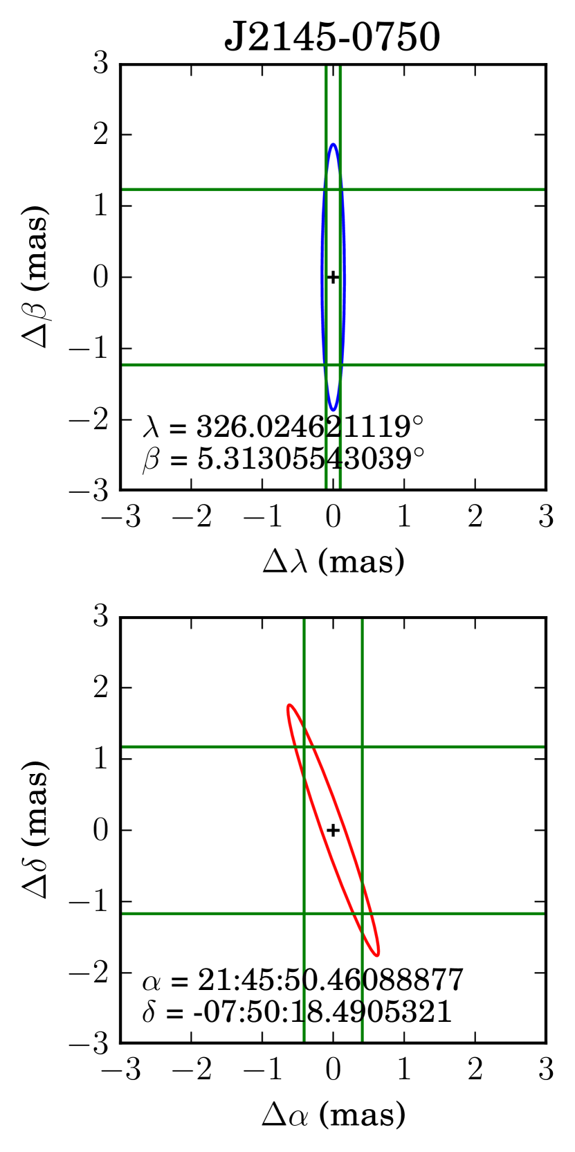
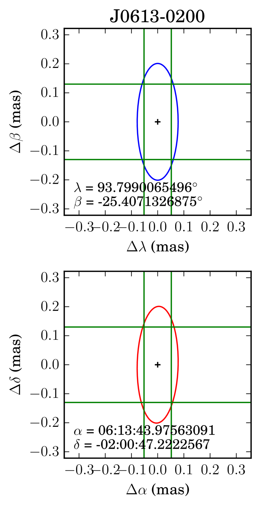
Figure 1.— Examples of $1\sigma$ error ellipses for pulsar position in equatorial coordinates, shown in red, and ecliptic coordinates, shown in blue. Green lines indicate $1\sigma$ uncertainties in mas, and hence they show the error region that can be inferred when the coordinates are reported in each coordinate system. For J2145-0750, $\sigma_{\lambda}=0.10$ mas, $\sigma_{\beta}=1.23$ mas, $\sigma_{\alpha}=0.41$ mas, and $\sigma_{\delta}=1.17$ mas. The error region is much larger in equatorial coordinates due to the covariance between right ascension and declination. For J0613-0200: $\sigma_{\lambda}=\sigma_{\alpha}=0.052$ mas, and $\sigma_{\beta}=\sigma_{\delta}=0.13$ mas, and the error regions are similar in size in the two coordinate systems. The severity of the covariance in equatorial coordinates, and hence the enlargement of the error ellipse when expressed in equatorial coordinates, depends on the pulsar’s ecliptic latitude and its proximity to the equinoxes.

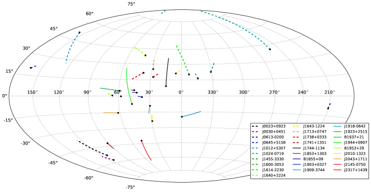
Figure 2.— Path of pulsar Galactic motion from 5 Myr ago to present, shown as black dots. Millisecond pulsars with greater than 5-sigma significant proper motion measured by NANOGrav are shown. Color and line style (solid or dashed) are used to identify individual pulsars but have no other significance.

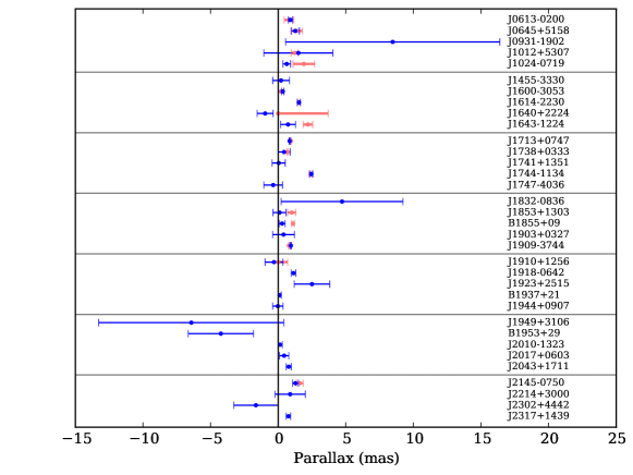
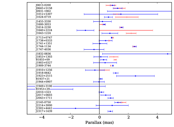
Figure 3.— Top: NANOGrav nine-year parallax values shown in blue in comparison to the previous best measurement or limit shown in faded red. Bottom: Top plot restricted to narrower parallax range.

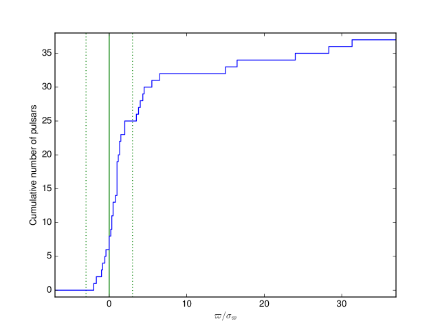
Figure 4.— Cumulative number of pulsars as a function of parallax measurement significance, $\varpi/\sigma_{\varpi}$. The dotted green lines delimit $\pm 3\sigma$.

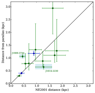
Figure 5.— Distances from parallax measurements versus distances from the NE2001 dispersion measure model for pulsars with significant parallax detections in our data set (upper part of Table 4). Parallax distances are plotted as $2\sigma$ uncertainties; NE2001 dispersion model distances are plotted with 25% uncertainties. Two pulsars for which there is no distance that is both within $2\sigma$ of the parallax distance and within 25% of the NE2001 distance are indicated by name and by light blue uncertainty boxes. Previous parallax measurements of PSRs J1713+0747 and J1744-1134 were used as input data to the NE2001 model; our measurements of these pulsars are shown in blue. All of our other measurements are shown in green.

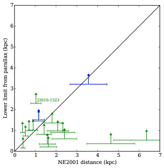
Figure 6.— Lower limits on distances from parallax measurements versus distances from the NE2001 dispersion measure model for pulsars without significant parallax detections in our data set (lower part of Table 4). Lower limit parallax distances are plotted as 95% confidence values; NE2001 dispersion model distances are plotted with 25% uncertainties. Previous parallax measurements or limits for PSRs B1855+09 and B1937+21 were used as input data to the NE2001 model; our limits for these pulsars are shown in blue. All of our other limits are shown in green.

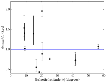
Figure 7.— Comparison of distances derived from dispersion measure via the NE2001 electron density model and parallax distances as a function of absolute Galactic latitude.

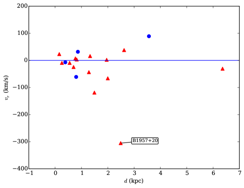
Figure 8.— Millisecond pulsar radial-velocities versus distance for pulsars whose radial velocity component was within $20^{\circ}$ of perpendicular to the line-of-sight. Isolated millisecond pulsars are shown as blue circles, while millisecond pulsars in binary systems are shown as red triangles.

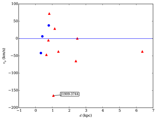
Figure 9.— Millisecond pulsar azimuthal-velocities versus distance for pulsars whose azimuthal velocity vector is within $\ 20^{\circ}$ of perpendicular to the line-of-sight. Isolated millisecond pulsars are sh own as blue circles, while millisecond pulsars in binary systems are shown as r ed triangles.

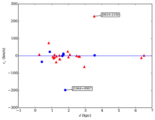
Figure 10.— Millisecond pulsar z-velocities versus distance for pulsars within $20^{\circ}$ latitude to the Galactic plane. Isolated millisecond pulsars are shown as blue circles, while millisecond pulsars in binary systems are shown as red triangles.

References

- Abdo et al. (2009) Abdo, A. A., Ackermann, M., Atwood, W. B., et al. 2009, ApJ, 699, 1171
- Abdo et al. (2013) Abdo, A. A., Ajello, M., Allafort, A., et al. 2013, ApJS, 208, 17
- Alpar et al. (1982) Alpar, M. A., Cheng, A. F., Ruderman, M. A., & Shaham, J. 1982, Nature, 300, 728
- Antoniadis et al. (2012) Antoniadis, J., van Kerkwijk, M. H., Koester, D., et al. 2012, MNRAS, 423, 3316
- Arzoumanian et al. (1994) Arzoumanian, Z., Fruchter, A. S., & Taylor, J. H. 1994, ApJ, 426, L85
- Arzoumanian et al. (2015) Arzoumanian, Z., Brazier, A., Burke-Spolaor, S., et al. 2015, ArXiv e-prints, arXiv:1505.07540
- Aumer & Binney (2009) Aumer, M., & Binney, J. J. 2009, MNRAS, 397, 1286
- Barr et al. (2013) Barr, E. D., Guillemot, L., Champion, D. J., et al. 2013, MNRAS, 429, 1633
- Bell & Bailes (1996) Bell, J. F., & Bailes, M. 1996, ApJ, 456, L33
- Binney & Merrifield (1998) Binney, J., & Merrifield, M. 1998, Galactic Astronomy (Princeton University Press)
- Callanan et al. (1998) Callanan, P. J., Garnavich, P. M., & Koester, D. 1998, MNRAS, 298, 207
- Camilo et al. (1996) Camilo, F., Nice, D. J., Shrauner, J. A., & Taylor, J. H. 1996, ApJ, 469, 819
- Champion et al. (2005) Champion, D. J., Lorimer, D. R., McLaughlin, M. A., et al. 2005, MNRAS, 363, 929
- Chatterjee et al. (2009) Chatterjee, S., Brisken, W. F., Vlemmings, W. H. T., et al. 2009, ApJ, 698, 250
- Cordes (2013) Cordes, J. M. 2013, in IAU Symposium, Vol. 291, IAU Symposium, ed. J. van Leeuwen, 211–216
- Cordes & Chernoff (1997) Cordes, J. M., & Chernoff, D. F. 1997, ApJ, 482, 971
- Cordes & Lazio (2002) Cordes, J. M., & Lazio, T. J. W. 2002, ArXiv Astrophysics e-prints, astro-ph/0207156
- Damour & Taylor (1991) Damour, T., & Taylor, J. H. 1991, ApJ, 366, 501
- Dawson & Schröder (2010) Dawson, S. A., & Schröder, K.-P. 2010, MNRAS, 404, 917
- Dehnen & Binney (1998) Dehnen, W., & Binney, J. J. 1998, MNRAS, 298, 387
- Deller et al. (2008) Deller, A. T., Verbiest, J. P. W., Tingay, S. J., & Bailes, M. 2008, ApJ, 685, L67
- Deller et al. (2012) Deller, A. T., Archibald, A. M., Brisken, W. F., et al. 2012, ApJ, 756, L25
- Deneva et al. (2012) Deneva, J. S., Freire, P. C. C., Cordes, J. M., et al. 2012, ApJ, 757, 89
- Du et al. (2014) Du, Y., Yang, J., Campbell, R. M., et al. 2014, ApJ, 782, L38
- Espinoza et al. (2013) Espinoza, C. M., Guillemot, L., Çelik, Ö., et al. 2013, MNRAS, 430, 571
- Folkner et al. (2009) Folkner, W. M., Williams, J. G., & Boggs, D. H. 2009, Interplanetary Network Progress Report, 178, C1
- Fonseca et al. (2014) Fonseca, E., Stairs, I. H., & Thorsett, S. E. 2014, ApJ, 787, 82
- Freire & Tauris (2014) Freire, P. C. C., & Tauris, T. M. 2014, MNRAS, 438, L86
- Freire et al. (2011) Freire, P. C. C., Bassa, C. G., Wex, N., et al. 2011, MNRAS, 412, 2763
- Freire et al. (2012) Freire, P. C. C., Wex, N., Esposito-Farèse, G., et al. 2012, MNRAS, 423, 3328
- Gonzalez et al. (2011) Gonzalez, M. E., Stairs, I. H., Ferdman, R. D., et al. 2011, ApJ, 743, 102
- Guillemot et al. (2012) Guillemot, L., Freire, P. C. C., Cognard, I., et al. 2012, MNRAS, 422, 1294
- Hobbs et al. (2005) Hobbs, G., Lorimer, D. R., Lyne, A. G., & Kramer, M. 2005, MNRAS, 360, 974
- Holmberg & Flynn (2004) Holmberg, J., & Flynn, C. 2004, MNRAS, 352, 440
- Hotan et al. (2006) Hotan, A. W., Bailes, M., & Ord, S. M. 2006, MNRAS, 369, 1502
- Hou et al. (2014) Hou, X., Smith, D. A., Guillemot, L., et al. 2014, A&A, 570, A44
- Janssen et al. (2010) Janssen, G. H., Stappers, B. W., Bassa, C. G., et al. 2010, A&A, 514, A74
- Kerr et al. (2012) Kerr, M., Camilo, F., Johnson, T. J., et al. 2012, ApJ, 748, L2
- Khargharia et al. (2012) Khargharia, J., Stocke, J. T., Froning, C. S., Gopakumar, A., & Joshi, B. C. 2012, ApJ, 744, 183
- Kiziltan & Thorsett (2010) Kiziltan, B., & Thorsett, S. E. 2010, ApJ, 715, 335
- Konacki & Wolszczan (2003) Konacki, M., & Wolszczan, A. 2003, ApJ, 591, L147
- Kuijken & Gilmore (1989) Kuijken, K., & Gilmore, G. 1989, MNRAS, 239, 571
- Lazaridis et al. (2009) Lazaridis, K., Wex, N., Jessner, A., et al. 2009, MNRAS, 400, 805
- Lazarus et al. (2015) Lazarus, P., Brazier, A., Hessels, J. W. T., et al. 2015, ArXiv e-prints, arXiv:1504.02294
- Leys et al. (2013) Leys, C., Ley, C., Klein, O., Bernard, P., & Licata, L. 2013, Journal of Experimental Social Psychology, 49, 764
- Löhmer et al. (2005) Löhmer, O., Lewandowski, W., Wolszczan, A., & Wielebinski, R. 2005, ApJ, 621, 388
- Lommen et al. (2006) Lommen, A. N., Kipphorn, R. A., Nice, D. J., et al. 2006, ApJ, 642, 1012
- Lorimer (2013) Lorimer, D. R. 2013, in IAU Symposium, Vol. 291, IAU Symposium, ed. J. van Leeuwen, 237–242
- Lorimer et al. (2007) Lorimer, D. R., McLaughlin, M. A., Champion, D. J., & Stairs, I. H. 2007, MNRAS, 379, 282
- Lorimer et al. (2006) Lorimer, D. R., Faulkner, A. J., Lyne, A. G., et al. 2006, MNRAS, 372, 777
- Lutz & Kelker (1973) Lutz, T. E., & Kelker, D. H. 1973, PASP, 85, 573
- Lynch et al. (2013) Lynch, R. S., Boyles, J., Ransom, S. M., et al. 2013, ApJ, 763, 81
- Manchester et al. (2005) Manchester, R. N., Hobbs, G. B., Teoh, A., & Hobbs, M. 2005, AJ, 129, 1993
- Ng et al. (2014) Ng, C., Bailes, M., Bates, S. D., et al. 2014, MNRAS, 439, 1865
- Nice et al. (2001) Nice, D. J., Splaver, E. M., & Stairs, I. H. 2001, ApJ, 549, 516
- Nice & Taylor (1995) Nice, D. J., & Taylor, J. H. 1995, ApJ, 441, 429
- Podsiadlowski et al. (2004) Podsiadlowski, P., Langer, N., Poelarends, A. J. T., et al. 2004, ApJ, 612, 1044
- Press et al. (2007) Press, W. H., Teukolsky, S. A., Vetterling, W. T., & Flannery, B. P. 2007, Numerical Recipes: The Art of Scientific Computing, 3nd edition (Cambridge: Cambridge University Press)
- Reid et al. (2014) Reid, M. J., Menten, K. M., Brunthaler, A., et al. 2014, ApJ, 783, 130
- Schnitzeler (2012) Schnitzeler, D. H. F. M. 2012, MNRAS, 427, 664
- Schönrich et al. (2010) Schönrich, R., Binney, J., & Dehnen, W. 2010, MNRAS, 403, 1829
- Sharma et al. (2014) Sharma, S., Bland-Hawthorn, J., Binney, J., et al. 2014, ApJ, 793, 51
- Shklovskii (1970) Shklovskii, I. S. 1970, Sov. Astron., 13, 562
- Splaver (2004) Splaver, E. M. 2004, PhD thesis, Princeton University
- Stovall et al. (2014) Stovall, K., Lynch, R. S., Ransom, S. M., et al. 2014, ApJ, 791, 67
- Sutaria et al. (2003) Sutaria, F. K., Ray, A., Reisenegger, A., et al. 2003, A&A, 406, 245
- Tauris & Bailes (1996) Tauris, T. M., & Bailes, M. 1996, A&A, 315, 432
- Tauris et al. (2012) Tauris, T. M., Langer, N., & Kramer, M. 2012, MNRAS, 425, 1601
- Tauris et al. (2013) Tauris, T. M., Sanyal, D., Yoon, S.-C., & Langer, N. 2013, A&A, 558, A39
- Toscano et al. (1999) Toscano, M., Sandhu, J. S., Bailes, M., et al. 1999, MNRAS, 307, 925
- van den Heuvel (2011) van den Heuvel, E. P. J. 2011, Bulletin of the Astronomical Society of India, 39, 1
- van Kerkwijk et al. (2011) van Kerkwijk, M. H., Breton, R. P., & Kulkarni, S. R. 2011, ApJ, 728, 95
- van Straten et al. (2012) van Straten, W., Demorest, P., & Oslowski, S. 2012, Astronomical Research and Technology, 9, 237
- Verbiest et al. (2010) Verbiest, J. P. W., Lorimer, D. R., & McLaughlin, M. A. 2010, MNRAS, 405, 564
- Verbiest et al. (2012) Verbiest, J. P. W., Weisberg, J. M., Chael, A. A., Lee, K. J., & Lorimer, D. R. 2012, ApJ, 755, 39
- Verbiest et al. (2008) Verbiest, J. P. W., Bailes, M., van Straten, W., et al. 2008, ApJ, 679, 675
- Verbiest et al. (2009) Verbiest, J. P. W., Bailes, M., Coles, W. A., et al. 2009, MNRAS, 400, 951
- Wolszczan et al. (2000) Wolszczan, A., Hoffman, I. M., Konacki, M., Anderson, S. B., & Xilouris, K. M. 2000, ApJ, 540, L41
- You et al. (2007) You, X. P., Hobbs, G., Coles, W. A., et al. 2007, MNRAS, 378, 493
- Zavlin (2006) Zavlin, V. E. 2006, ApJ, 638, 951
- Zhu et al. (2015) Zhu, W. W., Stairs, I. H., Demorest, P. B., et al. 2015, ArXiv e-prints, arXiv:1504.00662