Lorentz and CPT Violation in Top-Quark Production and Decay

Abstract

The prospects are explored for testing Lorentz and CPT symmetry in the top-quark sector. We present the relevant Lagrange density, discuss physical observables, and describe the signals to be sought in experiments. For top-antitop pair production via quark or gluon fusion with subsequent semileptonic or hadronic decays, we obtain the matrix element in the presence of Lorentz violation using the narrow-width approximation. The issue of testing CPT symmetry in the top-quark sector is also addressed. We demonstrate that single-top production and decay is well suited to a search for CPT violation, and we present the matrix elements for single-top production in each of the four tree-level channels. Our results are applicable to searches for Lorentz violation and studies of CPT symmetry in collider experiments, including notably high-statistics top-antitop and single-top production at the Large Hadron Collider.

I Introduction

The 1995 discovery of the top ($t$) quark at the Fermilab Tevatron d0cdf opened a new era for investigation of the Standard Model (SM) of particle physics. While experimental observations initially involved comparatively few events, the advent of the Large Hadron Collider (LHC) has radically changed the prospects for physics analyses involving the top quark. Indeed, the LHC can reasonably be viewed as a top-quark factory, since it is expected to produce several million single-top or single-antitop events and even more top-antitop pairs over the next few years, with ultimately another order of magnitude produced during the lifetime of the machine wb . The accompanying plethora of top-quark data, which is unlikely to be matched at another collider in the foreseeable future, offers a remarkable opportunity for precision measurements using the heaviest elementary fermion in the SM.

Most of the precision measurements involving the top quark that have been undertaken to date either attempt to verify basic predictions of the SM or search for new physics from models constructed within a conventional field-theoretic context. However, the high statistical power provided by the LHC dataset provides the opportunity to use top-quark physics to investigate profound issues involving the validity of underlying features of quantum field theory and the SM in the third generation. In the present work, we explore the prospects for studying the foundational Lorentz and CPT symmetries of the SM at the scale of the top quark.

Interest in precision tests of spacetime symmetries has grown significantly in recent years, following the observation that tiny violations of Lorentz and CPT invariance could arise naturally in an underlying unified theory such as strings and be described at accessible energy scales using effective field theory ksp . At this stage, numerous experiments using methods from a variety of subfields have sought evidence for Lorentz and CPT violation tables , but to date only one measurement investigating Lorentz symmetry in the top-quark sector has been performed D0top . Some theoretical motivation for top-quark studies comes from the notion that Lorentz violation in a complete spacetime theory involving gravity is expected to be spontaneous rather than explicit, as the latter is generically incompatible with conventional Riemann geometry or technically unnatural ak ; rb . Supposing that Lorentz violation indeed arises spontaneously through the vacuum expectation value of one or more tensor fields in the underlying theory, then the sizes of low-energy effects are governed in part by the couplings to these fields. If the latter follow the familiar pattern of Yukawa couplings in the SM determining the hierarchy of quark masses, then Lorentz- and CPT-violating effects might naturally be expected to be largest for the top quark. Moreover, since the top quark decays before hadronization, it offers a unique arena for studying Lorentz and CPT symmetry in essentially free quarks. In any case, independent of deeper potential theoretical motivations, as a matter of principle it is of interest to establish the laws of relativity for the top quark on as firm a footing as possible.

The comprehensive realistic effective field theory for Lorentz and CPT violation, called the Standard-Model Extension (SME), contains by construction the SM coupled to General Relativity along with all possible operators for Lorentz violation ak ; ck . In realistic effective field theories CPT violation is accompanied by Lorentz violation owg , so the SME also describes general CPT violation. A Lorentz-violating term in the Lagrange density of the SME is an observer scalar density formed by contracting a Lorentz-violating operator with a coefficient for Lorentz violation that controls the size of the associated effects. The operators can be classified systematically using their mass dimension $d$, with arbitrarily large values of $d$ appearing. The restriction of the SME to include only Lorentz-violating operators with $d\leq 4$, called the minimal SME, is a renormalizable theory in Minkowski spacetime. The SME provides a realistic and calculable framework for analyses of experimental data searching for deviations from Lorentz and CPT invariance reviews .

During recent years, many measurements have been performed of fundamental properties of the top quark, including its mass topmass , its charge topcharge , and its width topwidth . However, to date the sole search for Lorentz violation in the top-quark sector was performed by the D0 Collaboration D0top using data from the Fermilab Tevatron Collider and the theoretical formalism of the SME. The production of $t$-$\overline{t}$ pairs at the Tevatron is dominated by quark fusion, and the D0 Collaboration studied data corresponding to an integrated luminosity of 5.3 fb^-1 for processes with the $t$-$\overline{t}$ pairs decaying into leptonic and jet final states. These processes are primarily sensitive to certain dimensionless SME coefficients for CPT-even Lorentz violation, and the investigation constrains possible Lorentz violation involving these coefficients to below about the 10% level. The substantially greater statistical power available at the LHC offers the opportunity to improve significantly on this study. However, at the LHC the primary production mechanism for $t$-$\overline{t}$ pairs is gluon fusion, for which the matrix elements are different and more involved than those for quark fusion. One goal of the present work is to present the essential theory appropriate for $t$-$\overline{t}$ production by gluon fusion.

Another interesting issue is the extent to which CPT symmetry is respected by the top quark. Since CPT violation comes with Lorentz violation in realistic effective field theory ck ; owg , studies of CPT violation necessarily involve observables that change with energy and orientation. No experimental investigations of CPT symmetry for the top quark in this context have been performed to date. In this work, we partially address this gap in the literature by demonstrating that studies of single-top or single-antitop production at the LHC provide the basis for a search for CPT violation.

The structure of this paper is as follows. We begin in Sec. II by establishing the basic theory used in this work. The relevant parts of the SME Lagrange density are provided, the physical observables are identified, and the types of signals of relevance are discussed. We then turn in Sec. III to top-antitop pair production, where we present the matrix element for production and decay. The Lorentz-invariant result is given, followed by a demonstration that pair production is a CPT-even process. We give the explicit amplitudes for Lorentz-violating pair production and decay both via quark fusion, which was the dominant process for the D0 analysis, and via gluon fusion, which dominates at the LHC. In Sec. IV, we address CPT violation in the top-quark sector, showing that single-top production offers access to CPT observables. Four tree-level channels play a role, and we derive the matrix elements for each. Details of the spin sum required for calculations of the single-top matrix elements are relegated to appendix A. We conclude with a summary and discussion in Sec. V. Throughout this work, our conventions are those adopted in Ref. ck .

II Theory

This section provides some theoretical comments of relevance to the derivations in the remainder of the paper. We present the portion of the SME Lagrange density applicable to the top-quark searches studied here, discuss the issues of field redefinitions and physical observables, and offer some observations about generic signals that could be sought in experimental analyses.

II.1 SME Lagrange density for the top quark

In this paper, our focus is on the top-quark sector in the minimal SME. The part of the SME Lagrange density involving Lorentz and CPT violation in the top-quark sector can be extracted from Ref. ck . Denoting the left-handed quark doublets by $Q_{A}$ and the right-handed charge-2/3 singlets as $U_{A}$, the relevant piece of these equations describing CPT-even Lorentz violation is

$${\cal L}^{\rm CPT+} \supset {\textstyle{1\over 2}}i(c_{Q})_{\mu\nu AB}\overline{Q}_{A}\gamma^{\mu}\stackrel{{\scriptstyle\leftrightarrow}}{{D^{\nu}}}Q_{B}$$ (1)

$$+{\textstyle{1\over 2}}i(c_{U})_{\mu\nu AB}\overline{U}_{A}\gamma^{\mu}\stackrel{{\scriptstyle\leftrightarrow}}{{D^{\nu}}}U_{B}$$

$$-{\textstyle{1\over 2}}(H_{U})_{\mu\nu AB}\overline{Q}_{A}\phi^{c}\sigma^{\mu\nu}U_{B}+{\rm h.c.},$$

where $D_{\mu}$ is the gauge-covariant derivative and $\phi$ is the Higgs field. The piece governing CPT-odd Lorentz violation is

$${\cal L}^{\rm CPT-}\supset-(a_{Q})_{\mu AB}\overline{Q}_{A}\gamma^{\mu}Q_{B}-(a_{U})_{\mu AB}\overline{U}_{A}\gamma^{\mu}U_{B}.$$ (2)

The various coefficients in these equations determine the size of the Lorentz violation. The dimensionless coefficients $c_{\mu\nu AB}$ are traceless in spacetime indices $\mu,\nu$ and are hermitian in generation indices $A,B$, while the dimensionless coefficients $H_{\mu\nu AB}$ are antisymmetric in spacetime indices $\mu,\nu$. The coefficients $a_{\mu AB}$ have dimensions of mass and are hermitian in generation indices $A,B$.

In this work, which focuses on the top quark, we assume for definiteness and simplicity that the only relevant Lorentz and CPT violation involves the third generation, so that $A=B=3$. A more general treatment would also be of interest but lies outside our present scope. The coefficients of relevance here are therefore $(c_{Q})_{\mu\nu 33}$, $(c_{U})_{\mu\nu 33}$, $(H_{U})_{\mu\nu 33}$, $(a_{Q})_{\mu 33}$, and $(a_{U})_{\mu 33}$. The first three control CPT-even operators, while the last two control CPT-odd ones. All coefficients affect the propagator for the top-quark field $t$, while $(c_{Q})_{\mu\nu 33}$ and $(a_{Q})_{\mu 33}$ also affect the propagator for the bottom-quark field $b$, and $(c_{Q})_{\mu\nu 33}$ affects the $t$-$b$-$W$ vertex as well. For convenience in what follows, we introduce the abbreviated notation

$$(a_{L})_{\mu} = (a_{Q})_{\mu 33},\quad(a_{R})_{\mu}=(a_{U})_{\mu 33},$$

$$(c_{L})_{\mu\nu} = (c_{Q})_{\mu\nu 33},\quad(c_{R})_{\mu\nu}=(c_{U})_{\mu\nu 33},$$

$$H^{\prime}_{\mu\nu} = \langle{\phi}\rangle(H_{U})_{\mu\nu 33},\quad\widetilde{H}^{\prime}{}^{\mu\nu}={\textstyle{1\over 2}}\epsilon^{\mu\nu\rho\sigma}H^{\prime}_{\rho\sigma},$$ (3)

where $\langle{\phi}\rangle$ is the Higgs expectation value. It is also useful to define certain coefficient combinations as

$$a_{\mu} = {\textstyle{1\over 2}}[(a_{L})_{\mu}+(a_{R})_{\mu}],\quad b_{\mu}={\textstyle{1\over 2}}[(a_{L})_{\mu}-(a_{R})_{\mu}],$$

$$c_{\mu\nu} = {\textstyle{1\over 2}}[(c_{L})_{\mu\nu}+(c_{R})_{\mu\nu}],\quad d_{\mu\nu}={\textstyle{1\over 2}}[(c_{L})_{\mu\nu}-(c_{R})_{\mu\nu}],$$

$$H_{\mu\nu} = \hbox{Re}\,{H^{\prime}_{\mu\nu}}-\hbox{Im}\,{\widetilde{H}^{\prime}_{\mu\nu}}.$$ (4)

In these expressions, all coefficients are real except for $(H_{U})_{\mu\nu 33}$, $H^{\prime}_{\mu\nu}$, and its dual $\widetilde{H}^{\prime}{}^{\mu\nu}$, which may be complex.

For our purposes, the relevant part ${\cal L}_{t,b}^{\rm SM}$ of the matter Lagrange density for the conventional SM involves the $t$ and $b$ quark fields, their electroweak interactions with the $W^{\pm}_{\mu}$ bosons, and their strong interactions with the SU(3)-adjoint matrix $G_{\mu}$ of gluons. In what follows, the left- and right-handed fermion fields are defined by

$$\psi_{L}\equiv{\textstyle{1\over 2}}(1-\gamma_{5})\psi,\quad\psi_{R}\equiv{\textstyle{1\over 2}}(1+\gamma_{5})\psi,$$ (5)

as usual. Using this notation,

$${\cal L}_{t,b}^{\rm SM} = {\textstyle{1\over 2}}i\overline{t}\gamma^{\mu}\stackrel{{\scriptstyle\leftrightarrow}}{{\partial_{\mu}}}t-m_{t}\overline{t}t+{\textstyle{1\over 2}}i\overline{b}\gamma^{\mu}\stackrel{{\scriptstyle\leftrightarrow}}{{\partial_{\mu}}}b-m_{b}\overline{b}b$$ (6)

$$+({{gV_{tb}}\over{\sqrt{2}}}W_{\mu}^{-}\overline{b}_{L}\gamma^{\mu}t_{L}+{\rm h.c.})$$

$$+g_{\rm s}(\overline{t}\gamma^{\mu}G_{\mu}t+\overline{b}\gamma^{\mu}G_{\mu}b),$$

where $m_{t}$ and $m_{b}$ are the masses of the top and bottom quarks, respectively, $g$ is the electroweak coupling constant, $V_{tb}$ is an element of the Cabibbo-Kobayashi-Maskawa (CKM) matrix, and $g_{\rm s}$ is the strong coupling constant. The SME corrections involving CPT-even Lorentz violation can be extracted from Eq. (1) and written in various equivalent forms,

$${\cal L}^{\rm CPT+}_{t,b} = {\textstyle{1\over 2}}i(c_{L})_{\mu\nu}\overline{t}_{L}\gamma^{\mu}\stackrel{{\scriptstyle\leftrightarrow}}{{\partial^{\nu}}}t_{L}+{\textstyle{1\over 2}}i(c_{R})_{\mu\nu}\overline{t}_{R}\gamma^{\mu}\stackrel{{\scriptstyle\leftrightarrow}}{{\partial^{\nu}}}t_{R}$$ (7)

$$+{\textstyle{1\over 2}}i(c_{L})_{\mu\nu}\overline{b}_{L}\gamma^{\mu}\stackrel{{\scriptstyle\leftrightarrow}}{{\partial^{\nu}}}b_{L}$$

$$+({{gV_{tb}}\over{\sqrt{2}}}(c_{L})_{\mu\nu}W^{-\nu}\overline{b}_{L}\gamma^{\mu}t_{L}+{\rm h.c.})$$

$$-{\textstyle{1\over 2}}H_{\mu\nu}\overline{t}_{L}\sigma^{\mu\nu}t_{R}-{\textstyle{1\over 2}}H_{\mu\nu}\overline{t}_{R}\sigma^{\mu\nu}t_{L}$$

$$+g_{\rm s}c_{\mu\nu}(\overline{t}\gamma^{\mu}G^{\nu}t+\overline{b}\gamma^{\mu}G^{\nu}b),$$

$$= {\textstyle{1\over 2}}ic_{\mu\nu}\overline{t}\gamma^{\mu}\stackrel{{\scriptstyle\leftrightarrow}}{{\partial^{\nu}}}t+{\textstyle{1\over 2}}id_{\mu\nu}\overline{t}\gamma^{5}\gamma^{\mu}\stackrel{{\scriptstyle\leftrightarrow}}{{\partial^{\nu}}}t$$

$$+{\textstyle{1\over 2}}i(c_{L})_{\mu\nu}\overline{b}_{L}\gamma^{\mu}\stackrel{{\scriptstyle\leftrightarrow}}{{\partial^{\nu}}}b_{L}$$

$$+({{gV_{tb}}\over{\sqrt{2}}}(c_{L})_{\mu\nu}W^{-\nu}\overline{b}_{L}\gamma^{\mu}t_{L}+{\rm h.c.})$$

$$-{\textstyle{1\over 2}}H_{\mu\nu}\overline{t}\sigma^{\mu\nu}t+g_{\rm s}c_{\mu\nu}(\overline{t}\gamma^{\mu}G^{\nu}t+\overline{b}\gamma^{\mu}G^{\nu}b).\qquad$$

Similarly, the CPT-odd terms obtained from Eq. (2) can be written

$${\cal L}^{\rm CPT-}_{t,b} = -(a_{L})_{\mu}\overline{t}_{L}\gamma^{\mu}t_{L}-(a_{R})_{\mu}\overline{t}_{R}\gamma^{\mu}t_{R}$$ (8)

$$-(a_{L})_{\mu}\overline{b}_{L}\gamma^{\mu}b_{L}$$

$$= -a_{\mu}\overline{t}\gamma^{\mu}t-b_{\mu}\overline{t}\gamma^{5}\gamma^{\mu}t-(a_{L})_{\mu}\overline{b}_{L}\gamma^{\mu}b_{L}$$

$$= -a_{\mu}\overline{t}\gamma^{\mu}t-b_{\mu}\overline{t}\gamma^{5}\gamma^{\mu}t$$

$$-{\textstyle{1\over 2}}(a_{L})_{\mu}\overline{b}\gamma^{\mu}b-{\textstyle{1\over 2}}(a_{L})_{\mu}\overline{b}\gamma^{5}\gamma^{\mu}b.$$

In subsequent sections, the above expressions are used to derive the matrix elements for top-antitop production and decay and to explore the prospects for studying CPT violation in single-top production.

II.2 Observables

For top-quark production and decay, the Lorentz-violating terms listed above can affect Feynman diagrams through the production vertices, the $t$ and $\overline{t}$ propagators, the decay vertices, and the $b$ and $\overline{b}$ propagators. At leading order, each contribution from Lorentz violation arises as an insertion on a propagator or a vertex. The matrix element for a Lorentz-violating process can then be computed from the Feynman diagrams in the usual way, except perhaps for some technical issues involving external legs extleg . However, only a subset of the Lorentz-violating insertions lead to physically observable effects. Some terms can be absorbed into unobservable phases in the fields, choices for the spacetime coordinates, or redefinitions of the spinor basis ck ; ak ; akmm ; redefref . These terms therefore can be expected to cancel in matrix elements. To minimize calculations, it is useful to identify relevant terms beforehand. In this subsection, we outline the procedure for this.

For the analysis, one could in principle work with the SME prior to the SU(2)$\times$U(1) breaking, at the level of Eqs. (1) and (2). The relevant spinor fields subject to redefinitions would then be $Q_{A}$ and $U_{A}$, but care must be taken because the two components of each quark doublet can play independent roles. Here, we work instead with the terms (7) and (8) belonging to the SME Lagrange density after the SU(2)$\times$U(1) breaking, for which the relevant spinor fields are $t_{L}$, $t_{R}$, $b_{L}$, $b_{R}$. It suffices for present purposes to consider the observability of coefficients at leading order.

Consider first the terms (7) for CPT-even Lorentz violation. Each coefficient of the $c_{\mu\nu}$ and $d_{\mu\nu}$ type is a sum of three observer Lorentz irreducible pieces: a trace, a symmetric part, and an antisymmetric part. The traces of these coefficients are irrelevant for our purposes because they are Lorentz invariant and can be absorbed into overall normalizations of the fields, so they can be set to zero without loss of generality. Also, the symmetric parts of these coefficients are all physically observable in principle. Specifying the particle sector used to define the Minkowski metric normally removes one symmetric coefficient of the $c_{\mu\nu}$ type, but in the present instance we have already tacitly made such a choice by assuming that the light quark sectors are conventional. In contrast, only some of the antisymmetric parts of the coefficients of the $c_{\mu\nu}$ and $d_{\mu\nu}$ type can be physically observable due to the possibility of field redefinitions amounting to a choice of basis in spinor space.

As an explicit example, consider the redefinition $t_{L}\to(1+iv_{\mu\nu}\sigma^{\mu\nu})t_{L}$ where $v_{\mu\nu}$ is constant, and perform the same redefinition on $t_{R}$, $b_{L}$, $b_{R}$. We remark that although this redefinition superficially resembles an infinitesimal Lorentz transformation under which the Lagrange density is invariant, here only a subset of the fields are involved and so the form of the Lagrange density changes. Under this redefinition, the kinetic term for $t$ in Eq. (6) generates a term of the $c_{\mu\nu}$ type for $t$, while the $t$ mass term is invariant. Similarly, the $b$ kinetic term generates a term of the $c_{\mu\nu}$ type for $b$, and the $b$ mass term is invariant. The $W^{-}_{\mu}$ interaction term produces an interaction term involving $(c_{L})_{\mu\nu}$, while the gluon couplings are invariant. These results imply that all the antisymmetric parts of $c_{\mu\nu}$ appearing in Eq. (7) can be absorbed by a suitable choice of $v_{\mu\nu}$, at the cost of introducing a term of the form $i(c_{L})_{\mu\nu}\overline{b}_{R}\gamma^{\mu}\stackrel{{\scriptstyle\leftrightarrow}}{{\partial^{\nu}}}b_{R}$ for the $b_{R}$ field. It then follows, for example, that the antisymmetric part of $c_{\mu\nu}$ is irrelevant for top-quark production, and also that any effects on top decays can be attributed to the propagator terms for $b$ and $\overline{b}$. A similar line of reasoning reveals that the antisymmetric part of $d_{\mu\nu}$ can be absorbed into $H_{\mu\nu}$ and elsewhere in the Lagrange density, so it can therefore be viewed as irrelevant for present purposes as well.

Next, consider the terms (8) for CPT-odd Lorentz violation. Suppose first that $t_{L}$ is redefined by an unobservable position-dependent phase, $t_{L}\to\exp(-iv_{\mu}x^{\mu})t_{L}$, where $v_{\mu}$ is constant. The mass term for $t$ in Eq. (6) remains unaffected provided $t_{R}$ is redefined the same way. The kinetic term for $t$ in the SM Lagrange density then generates a term of the $a_{\mu}$ type for $t$. The $W_{\mu}^{-}$-interaction term is invariant if $b_{L}$ is redefined in this way, and the mass term for $b$ is unchanged if $b_{R}$ is too. The kinetic term for $b$ in the SM Lagrange density then generates a term of the $a_{\mu}$ type for $b$. These results imply that the freedom in choosing $v_{\mu}$ allows, for example, removing the term $-{\textstyle{1\over 2}}(a_{L})_{\mu}\overline{b}\gamma^{\mu}b$ from the last line of Eq. (8) without loss of generality. A useful option is to choose $v_{\mu}$ to cancel $(a_{L})_{\mu}$ in the first and third terms of the first line of Eq. (8), leaving the physically equivalent terms

$${\cal L}^{\rm CPT-}_{t,b} \equiv [(a_{L})_{\mu}-(a_{R})_{\mu}]\overline{t}_{R}\gamma^{\mu}t_{R}+(a_{L})_{\mu}\overline{b}_{R}\gamma^{\mu}b_{R}$$ (9)

$$= b_{\mu}\overline{t}\gamma^{\mu}t-b_{\mu}\overline{t}\gamma^{5}\gamma^{\mu}t$$

$$+{\textstyle{1\over 2}}(a_{L})_{\mu}\overline{b}\gamma^{\mu}b-{\textstyle{1\over 2}}(a_{L})_{\mu}\overline{b}\gamma^{5}\gamma^{\mu}b$$

in which only right-handed fields appear.

With the above choices, the description of CPT violation in the top-quark sector is reduced to considerations of insertions involving only right-handed fields, thereby simplifying both practical calculations and physical intuition. For the latter, for example, with the effects of CPT violation limited to the $t$ propagator according to Eq. (9), a top quark follows a geodesic in a pseudo-Finsler spacetime finsler . In a related vein, we remark in passing that no mass differences between $t$ and $\overline{t}$ appear, a result in accordance with Greenberg’s theorem owg and also with expectations for CPT violation in realistic effective field theory, where the antitop particle associated with the field $\overline{t}$ is defined as the antiparticle of $t$ and therefore by construction always has the same Lagrange-density mass.

Further simplifications affecting the observability of CPT violation appear if one or more of the quark masses can be neglected in a given process. For example, when the $b$ mass $m_{b}$ is negligible compared to the $b$ kinetic term, then the field $b_{R}$ can be independently redefined using a different phase, $b_{R}\to\exp(-iv^{\prime}_{\mu}x^{\mu})b_{R}$, while leaving unaffected the form of the SM Lagrange density except for generating a term of the $a_{\mu}$ type for $b$. A suitable choice of $v^{\prime}$ therefore can eliminate all $b$-quark terms in Eq. (9) when $m_{b}$ is negligible. Any observable CPT-violating effects on $t$ processes must then arise from insertions on $t$-quark propagators. Moreover, if the $t$ mass $m_{t}$ itself is also negligible in a given experimental process, then all $t$-quark terms in Eq. (9) can be removed via another independent field redefinition without changing the physics. For this special limiting case and under the assumptions leading to Eqs. (6) and (8), no top-quark CPT violation is observable at leading order.

II.3 Signals

Top-quark physics offers a rich variety of options for seeking Lorentz-invariant physics beyond the SM beyondSM . However, signals of Lorentz violation have unique features that cannot be associated with Lorentz-invariant effects. For example, in a given inertial frame, the presence of Lorentz violation means that the properties of each quark depend on its direction of travel and its boost. Moreover, if the Lorentz violation includes CPT violation, then the properties of the top and antitop can differ as well. These features lead to distinctive experimental signals that provide a basis for searches for Lorentz violation in the top-quark sector, as outlined in this subsection.

For ease of comparison between experiments, it is useful to introduce a standard inertial frame to report measurements of coefficients for Lorentz violation. The canonical frame adopted in the literature is a Sun-centered frame tables ; akmm ; sunframe . Cartesian coordinates $(T,X,Y,Z)$ in this frame are defined so that the $Z$ axis points along the direction of the Earth’s rotation, while the $X$ axis points from the Earth to the Sun at the vernal equinox 2000. Unlike any Earth-based reference frame, the Sun-centered frame can be taken as approximately inertial over a period of years. Its alignment also means that the transformation between the Sun-centered frame and a laboratory frame is comparatively simple. Suppose, for example, that cartesian coordinates $(t,x,y,z)$ in the laboratory are chosen such that the $x$-axis points south, the $y$-axis points east, and the $z$-axis points vertically upwards. Since the Earth rotates with sidereal frequency $\omega_{\oplus}\simeq 2\pi$/(23 h 56 m) the relationship mapping coefficients in the laboratory frame to those in the Sun-centered frame involves a time-dependent rotation $R^{jJ}$ between the two coordinate systems, which is given explicitly as akmm

$$R^{jJ}=\left(\begin{array}[]{ccc}\cos\chi\cos\omega_{\oplus}T&\cos\chi\sin\omega_{\oplus}T&-\sin\chi\\ -\sin\omega_{\oplus}T&\cos\omega_{\oplus}T&0\\ \sin\chi\cos\omega_{\oplus}T&\sin\chi\sin\omega_{\oplus}T&\cos\chi\end{array}\right),$$ (10)

where $\chi$ is the colatitude of the experiment.

For convenience of use, the expressions derived in the sections below for the various matrix elements for top-quark production and decay are expressed as observer Lorentz scalars, so they can be evaluated in any observer frame. For example, the laboratory frame can be chosen as the specified observer frame, and then the expressions for the matrix elements can be evaluated with all coefficients and 4-momenta taken in that frame. Since the coefficients in the laboratory frame can be obtained from those in the Sun-centered frame via the rotation (10), experimental results can readily be reported directly in terms of coefficients in the Sun-centered frame. The reader is cautioned here to distinguish the observer Lorentz invariance, which is merely an expression of coordinate independence of the physics, from the physical particle Lorentz violation arising through nonzero coefficients ck . For example, in the presence of Lorentz violation, physically boosting a particle of mass $m$ in any fixed observer frame produces behavior governed by a modified dispersion relation involving coefficients for Lorentz violation kl01 , instead of the standard dispersion relation $p^{2}=m^{2}$.

It is physically reasonable to take the coefficients for Lorentz violation as constant in the Sun-centered frame aksidereal . Since the transformation to the laboratory frame involves the time-dependent rotation (10), the laboratory-frame coefficients vary with sidereal time. Lorentz violation therefore can be expected to produce sidereal oscillations in the data, with amplitudes and phases governed by the coefficients for Lorentz violation. Most coefficients produce signals at the sidereal frequency $\omega_{\oplus}$, but the symmetric components of the coefficient $c_{\mu\nu}$ generate ones at the harmonic $2\omega_{\oplus}$ as well. Note also that the revolution of the Earth about the Sun introduces an extra time dependence in the laboratory-frame coefficients with an annual periodicity. However, this time dependence is suppressed relative to the previous one by the Earth’s boost $\beta_{\oplus}\simeq 10^{-4}$, which in practice reduces the experimental sensitivity to annual variations to below the level of interest here.

The above considerations reveal that the data for top-quark production and decay can be expected to contain information in the amplitudes and phases of the the sidereal and twice-sidereal harmonics. An analysis including many coefficients can be cumbersome, but in practice considerable insight can be gained by allowing only one component of a coefficient for Lorentz violation to be nonzero at a time, and extracting the sensitivity to it. This simplified procedure is common practice in the field tables . While it disregards possible interference or cancellation of effects between coefficient components, it does give a notion of the maximal sensitivity achieved to each component. Evidently, if a nonzero result is found for any component, the question of possible interference would need to be revisited. This type of analysis has been performed recently in the context of top-antitop production by the D0 Collaboration D0top , who report limits of about 10% on individual components of the $c_{\mu\nu}$-type coefficients in the canonical Sun-centered frame.

In addition to studying sidereal signals, which intrinsically include both CPT-even and CPT-odd Lorentz violation, an analysis can also seek to isolate CPT-odd effects. One method to achieve this is to work with a suitable asymmetry. If the rate for a process is found to be $R$ and the rate for the CPT-conjugate process is $\overline{R}$, then the asymmetry

$${\cal A}_{\rm CPT}\equiv{{R-\overline{R}}\over{R+\overline{R}}}$$ (11)

provides a measure of CPT violation for that process. Asymmetries of this type have been widely used in the context of SME studies of CPT violation in neutral-meson oscillations aksidereal ; akrvk , where coefficients for various combinations of non-top quarks have been experimentally constrained using $K^{0}$, $D^{0}$, $B^{0}_{d}$, and $B^{0}_{s}$ mesons KTEV ; KLOE ; FOCUS ; BABAR ; D0 . The asymmetry ${\cal A}_{\rm CPT}$ is proportional to coefficients for CPT-odd Lorentz violation, and typically it has both a constant term and a term oscillating with sidereal time. The experimental analysis therefore has several paths available to extract different information. Constructing the time-averaged asymmetry $\langle{{\cal A}_{\rm CPT}}\rangle$, for which oscillations average to zero over many sidereal days, permits constraints on coefficients enterng the constant term, while studying the amplitudes and phases of the oscillations provides independent measures of CPT symmetry.

III Top-antitop pair production

In this section we discuss the matrix elements for top-antitop pair production in the presence of Lorentz violation. We begin by outlining the Lorentz-invariant case, including top-antitop pair production both from quark fusion and from gluon fusion. We then consider the Lorentz-violating situation, showing that the process is CPT even and deriving the matrix elements for both quark fusion and gluon fusion at leading order in Lorentz violation.

III.1 Lorentz-invariant case

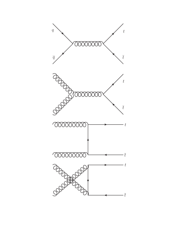
Figure 1: Tree-level Feynman diagrams for $t$-$\overline{t}$ production via quark fusion ($q\overline{q}\to t\overline{t}$) and gluon fusion ($gg\to t\overline{t}$).

Consider first the matrix element ${\cal M}$ for the case without Lorentz violation. The process of interest involves the production of a $t$-$\overline{t}$ pair, each component of which then decays. In quark fusion the production is via a single gluon in the $s$ channel, while in gluon fusion all three $s$, $t$, and $u$ channels contribute. The tree-level diagrams of relevance are shown in Fig. 1. Note that production via gluon fusion contributes only at the 15% level at Tevatron energies knk , while for production at LHC energies the situation is reversed with gluon fusion dominating the process.

In the standard narrow-width approximation nwa ; Berdine:2007uv ; Uhlemann:2008pm , the squared modulus of ${\cal M}$ can be written as the product of three parts,

$$|{\cal M}|^{2}=PF\overline{F}.$$ (12)

The quantities $P$, $F$, and $\overline{F}$ represent the factors from the $t$-$\overline{t}$ pair production, the $t$ decay, and the $\overline{t}$ decay, respectively. Next, we consider each factor in turn.

The production factor $P$ is different for quark fusion and gluon fusion. For quark fusion the production factor $P_{q\overline{q}}$ is given by

$$P_{q\overline{q}} = {g_{\rm s}^{4}\over 9}(2-\beta^{2}\sin^{2}\theta)$$ (13)

$$= {g_{\rm s}^{4}\over{18E^{4}}}\Big{[}(p_{q}\cdot p_{t})(p_{\overline{q}}\cdot p_{\overline{t}})+(p_{q}\cdot p_{\overline{t}})(p_{\overline{q}}\cdot p_{t})$$

$$\quad\qquad+(p_{q}\cdot p_{\overline{q}})m_{t}^{2}\Big{]},$$

where $\beta$ is the common speed of the $t$ and $\overline{t}$ quarks in the production center-of-mass frame, and $\theta$ is the scattering angle. The second equation above provides the expression in terms of the four-momenta of the various particles involved, with $E$ being the common energy of the quark or antiquark in the production center-of-mass frame, so that the usual Mandelstam variable for the subprocess is $s=4E^{2}$.

For gluon fusion, the production factor $P_{2g}$ with color and polarization averaged and spins summed can be expressed as a sum of six contributions arising from the three Feynman diagrams in the $s$, $t$, and $u$ channels Gluck:1977 ; Combridge:1978kx ; Ellis:1991qj ,

$$P_{2g} = \overline{\sum}\big{(}|{\cal M}_{ss}|^{2}+|{\cal M}_{tt}|^{2}+|{\cal M}_{uu}|^{2}$$ (14)

$$\qquad+|{\cal M}_{st}|^{2}+|{\cal M}_{su}|^{2}+|{\cal M}_{tu}|^{2}\big{)},$$

where

$$\overline{\sum}|{\cal M}_{ss}|^{2}={{3g_{\rm s}^{4}}\over 4}{{(t-m_{t}^{2})(u-m_{t}^{2})}\over{s^{2}}},$$

$$\overline{\sum}|{\cal M}_{tt}|^{2}={{g_{\rm s}^{4}}\over 6}{{(t-m_{t}^{2})(u-m_{t}^{2})-2m_{t}^{2}(t+m_{t}^{2})}\over{(t-m_{t}^{2})^{2}}},$$

$$\overline{\sum}|{\cal M}_{uu}|^{2}={{g_{\rm s}^{4}}\over 6}{{(u-m_{t}^{2})(t-m_{t}^{2})-2m_{t}^{2}(u+m_{t}^{2})}\over{(u-m_{t}^{2})^{2}}},$$

$$\overline{\sum}|{\cal M}_{st}|^{2}={{3g_{\rm s}^{4}}\over 8}{{(t-m_{t}^{2})(u-m_{t}^{2})+m_{t}^{2}(u-t)}\over{s(t-m_{t}^{2})}},$$

$$\overline{\sum}|{\cal M}_{su}|^{2}={{3g_{\rm s}^{4}}\over 8}{{(u-m_{t}^{2})(t-m_{t}^{2})+m_{t}^{2}(t-u)}\over{s(u-m_{t}^{2})}},$$

$$\overline{\sum}|{\cal M}_{tu}|^{2}=-{{g_{\rm s}^{4}}\over{24}}{{m_{t}^{2}(s-4m_{t}^{2})}\over{(t-m_{t}^{2})(u-m_{t}^{2})}}.$$ (15)

In these expressions, $s$, $t$, and $u$ are the usual Mandelstam variables,

$$s = (p_{1}+p_{2})^{2}=(p_{t}+p_{\overline{t}})^{2}$$

$$= 2p_{1}\cdot p_{2}=2p_{t}\cdot p_{\overline{t}}+2m_{t}^{2},$$

$$t = (p_{2}-p_{t})^{2}=(p_{1}-p_{\overline{t}})^{2}$$

$$= -2p_{2}\cdot p_{t}+m_{t}^{2}=-2p_{1}\cdot p_{\overline{t}}+m_{t}^{2},$$

$$u = (p_{1}-p_{t})^{2}=(p_{2}-p_{\overline{t}})^{2}$$ (16)

$$= -2p_{1}\cdot p_{t}+m_{t}^{2}=-2p_{2}\cdot p_{\overline{t}}+m_{t}^{2},$$

where $p_{1}$, $p_{2}$ are the 4-momenta of the two gluons. Each of the six expressions above represents either the squared modulus of an individual diagram or the interference between different channels. The calculation uses the trick of modifying the $s$-channel diagram to remove the contribution of the unphysical gluon polarizations Combridge:1978kx ; Feynman:1963ax ; Georgi:1978kx . If instead the unphysical polarizations are handled by including the contribution from Fadeev-Popov ghosts in the squared matrix elements, then the individual expressions above differ but their sum remains unchanged.

Within the narrow-width approximation, the decay factors $F$, $\overline{F}$ are independent of the production mechanism. Suppose for definiteness that the $t$ decays leptonically as

$$t\to W^{+}b\to\overline{l}\nu b$$ (17)

while the $\overline{t}$ decays hadronically as

$$\overline{t}\to W^{-}\overline{b}\to q\overline{q}^{\prime}\overline{b}.$$ (18)

The factor $F$ in Eq. (12) is then given by mp97

$$F={{g^{4}}\over 4}{{(m_{i}^{2}-m_{\overline{l}\nu}^{2})}\over{(m_{t}\Gamma_{t})^{2}}}\left[{{m_{i}^{2}(1-c_{\overline{l}b}^{2})+m_{\overline{l}\nu}^{2}(1+c_{\overline{l}b})^{2}}\over{(m_{\overline{l}\nu}^{2}-m_{W}^{2})^{2}+(m_{W}\Gamma_{W})^{2}}}\right]$$ (19)

while the factor $\overline{F}$ is given by

$$\overline{F}={{g^{4}}\over 4}{{(\overline{m}_{i}^{2}-m_{q\overline{q}^{\prime}}^{2})}\over{(m_{t}\Gamma_{t})^{2}}}\left[{{\overline{m}_{i}^{2}(1-c_{q\overline{b}}^{2})+m_{q\overline{q}^{\prime}}^{2}(1+c_{q\overline{b}})^{2}}\over{(m_{q\overline{q}^{\prime}}^{2}-m_{W}^{2})^{2}+(m_{W}\Gamma_{W})^{2}}}\right].$$ (20)

In these expressions, $m_{\overline{l}\nu}$ is the invariant mass of the lepton and neutrino from the $W^{+}$ decay, and $m_{q\overline{q}^{\prime}}$ is the 2-jet invariant mass from the $W^{-}$ decay. Also, $m_{i}$ is the invariant mass of the lepton, neutrino, and $b$ from the $t$ decay, while $\overline{m}_{i}$ is the 3-jet invariant mass from the $\overline{t}$ decay. The width of the $t$ quark is denoted by $\Gamma_{t}$, while the mass and width of the $W$ boson are $m_{W}$ and $\Gamma_{W}$. The quantity $c_{\overline{l}b}$ is the cosine of the angle between the lepton and the $b$ in the $W^{+}$ rest frame, and $c_{q\overline{b}}$ is the cosine of the angle between the light quarks from the $W^{-}$ and the $\overline{b}$ in the $W^{-}$ rest frame. For simplicity, we have omitted the CKM factors. To describe the top line shape, a correction to the denominator $(m_{t}\Gamma_{t})^{2}$ can be introduced d0-peak , which in principle would involve the modified top dispersion relation. In terms of four-momenta, the quantities $F$ and $\overline{F}$ become

$$F = -4g^{4}{{(p_{\nu}\cdot p_{b})(p_{\overline{\ell}}\cdot p_{t})}\over{(m_{t}\Gamma_{t})^{2}[(m_{\overline{\ell}\nu}^{2}-m_{W}^{2})^{2}+(m_{W}\Gamma_{W})^{2}]}}~{},$$

$$\overline{F} = -4g^{4}{{(p_{q}\cdot p_{b})(p_{\overline{q}^{\prime}}\cdot p_{\overline{t}})}\over{(m_{t}\Gamma_{t})^{2}[(m_{q\overline{q}^{\prime}}^{2}-m_{W}^{2})^{2}+(m_{W}\Gamma_{W})^{2}]}}.$$

For other decays of the $t$ and $\overline{t}$, the corresponding decay-product momenta can be substituted appropriately.

III.2 Lorentz-violating case

In the presence of Lorentz violation, additional Feynman diagrams contribute to the matrix element for $t$-$\overline{t}$ production and decay. As before, the narrow-width approximation factors the matrix element into a production part and two decay parts. The additional contributions to the Feynman diagrams for each of these parts arise as Lorentz-violating insertions on the propagators and vertices, in accordance with the general discussion given in Sec. II.2. The effects of each type of coefficient can be considered in turn.

Consider first the prospective contributions from the coefficients associated with CPT violation, which are contained in the Lagrange-density terms (8) or, equivalently, in Eq. (9). It turns out that these coefficients produce no relevant effects, as can be seen in several ways. A general line of reasoning considers the production process $q\overline{q}\to t\overline{t}$ or $gg\to t\overline{t}$ at all orders, assuming no polarizations or spins are detected. If this process were CPT violating, then its squared amplitude would necessarily have a contribution proportional to an odd power of coefficients for CPT violation and therefore should change sign under the CPT operation. However, the CPT-conjugate squared amplitude can be obtained by interchanging $q\leftrightarrow\overline{q}$ for all quarks including the top, which by inspection of the generic Feynman diagram yields the same squared amplitude as the original process. This is impossible unless no CPT violation occurs.

To understand more explicitly why CPT violation has no relevant effect for unpolarized $t$-$\overline{t}$ production and decay, we can consider various specific insertions in turn. Using the first line of Eq. (9), for example, we see that CPT violation involves only right-handed $t$ or $b$ fields. Inspection reveals that every diagram with a corresponding insertion on a $t$ or $b$ propagator is accompanied by a conjugate diagram yielding a contribution of the same magnitude but opposite sign. This cancellation also holds in the context of the narrow-width approximation. We can therefore disregard CPT violation in $t$-$\overline{t}$ production and decay without loss of generality.

Next, consider effects involving the coefficients associated with CPT-even Lorentz-violating operators given by Eq. (7). Consider first the coefficient $H_{{\mu\nu}}$. Insertion of the associated operator on the production side gives a vanishing matrix element. Insertion in the decay diagrams gives a nonzero matrix element, but the result vanishes when the phase-space integral is performed for the $t$ and $\overline{t}$ decays. This suggests that insertion of the $H_{{\mu\nu}}$ operator generates spin-correlation effects, which can be neglected for present purposes. Any real effects of this type could in principle be observed as angular information in the final state, but they are suppressed by the coefficients for Lorentz violation relative to the usual spin correlations that exist in the Lorentz-invariant top-quark production and decay and hence are unlikely to be candidates for precision measurement.

The Lorentz-violating contributions of interest are therefore those involving the $c_{\mu\nu}$-type coefficients. To express these effects, we write the square of the matrix element at first order in Lorentz violation in the form

$$|{{\cal M}}|^{2} = PF\overline{F}+(\delta_{p}P)F\overline{F}+(\delta_{v}P)F\overline{F}$$ (22)

$$+P(\delta F)\overline{F}+PF(\delta\overline{F}).$$

The first term is the Lorentz-invariant piece given in the previous section, while the other terms represent the corrections arising at leading order in the $c_{\mu\nu}$-type coefficients. The subscripts $p$ and $v$ refer to propagator and vertex insertions, respectively. In what follows, we discuss each of the Lorentz-violating corrections in turn.

III.2.1 Production via quark fusion

For production via quark fusion, the corrections can conveniently be expressed in terms of the coefficient $c_{\mu\nu}$ introduced in Eq. (4). The contribution from insertions on the $t$ and $\overline{t}$ propagators is

$$\delta_{p}P = {g_{\rm s}^{4}\over{18E^{4}}}c_{\mu\nu}\Big{[}(p_{q}\cdot p_{t})(p_{\overline{t}}^{\mu}p_{\overline{q}}^{\nu})+(p_{q}\cdot p_{\overline{t}})(p_{t}^{\mu}p_{\overline{q}}^{\nu})$$ (23)

$$+(p_{\overline{q}}\cdot p_{t})(p_{\overline{t}}^{\mu}p_{q}^{\nu})+(p_{\overline{q}}\cdot p_{\overline{t}})(p_{t}^{\mu}p_{q}^{\nu})\Big{]}.$$

The contribution from the production vertex is

$$\delta_{v}P = {g_{\rm s}^{4}\over{18E^{4}}}c_{\mu\nu}\Big{[}-(p_{q}\cdot p_{\overline{q}})(p_{t}^{\mu}p_{\overline{t}}^{\nu}+p_{\overline{t}}^{\mu}p_{t}^{\nu})$$ (24)

$$-(p_{t}\cdot p_{\overline{t}}+m_{t}^{2})(p_{q}^{\mu}p_{\overline{q}}^{\nu}+p_{\overline{q}}^{\mu}p_{q}^{\nu})$$

$$+(p_{q}\cdot p_{t})p_{\overline{q}}^{\mu}p_{\overline{t}}^{\nu}+(p_{q}\cdot p_{\overline{t}})p_{\overline{q}}^{\mu}p_{t}^{\nu}$$

$$+(p_{\overline{q}}\cdot p_{t})p_{q}^{\mu}p_{\overline{t}}^{\nu}+(p_{\overline{q}}\cdot p_{\overline{t}})p_{q}^{\mu}p_{t}^{\nu}\Big{]}.$$

The above expressions have been used by the D0 Collaboration to perform a search for Lorentz violation in the top-quark sector using data from the Fermilab Tevatron D0top . In principle, the statistical power of this analysis could be enhanced by incorporating also the production from gluon fusion described in the next section, which would give additional contributions suppressed at the 15% level relative to the ones above knk .

III.2.2 Production via gluon fusion

For production via gluon fusion, the correction from the propagators can be separated into six parts, three coming from squaring the amplitude of each Feynman diagram and three from the interference between the amplitudes of diagram pairs. These six contributions represent the dominant ones for $t$-$\overline{t}$ production at LHC energies and hence are well suited for a Lorentz-violation search using data from the LHC detectors.

Adopting the same notation as in Eq. (16), the squared moduli for the $s$, $t$, and $u$ channels give the three contributions

$$\delta_{p}\overline{\sum}|{\cal M}_{ss}|^{2} = {{3g_{\rm s}^{4}c_{\mu\nu}}\over{4s^{2}}}\big{[}s(p_{t}^{\mu}p_{\overline{t}}^{\nu}+p_{\overline{t}}^{\mu}p_{t}^{\nu})+(t-m_{t}^{2})(p_{1}^{\mu}p_{\overline{t}}^{\nu}+p_{2}^{\mu}p_{t}^{\nu})\ +(u-m_{t}^{2})(p_{1}^{\mu}p_{t}^{\nu}+p_{2}^{\mu}p_{\overline{t}}^{\nu})\big{]},$$ (25)

$$\delta_{p}\overline{\sum}|{\cal M}_{tt}|^{2} = {{g_{\rm s}^{4}c_{\mu\nu}}\over{6(t-m_{t}^{2})^{3}}}\big{[}(-t^{2}+tu-m_{t}^{2}u+3m_{t}^{2}t-10m_{t}^{4})(p_{1}^{\mu}p_{2}^{\nu}+p_{2}^{\mu}p_{1}^{\nu})$$ (26)

$$\hskip 50.0pt+(t^{2}+tu-m_{t}^{2}u-9m_{t}^{2}t)(p_{t}^{\mu}p_{\overline{t}}^{\nu}+p_{\overline{t}}^{\mu}p_{t}^{\nu})$$

$$\hskip 50.0pt+(-t^{2}-tu+m_{t}^{2}u+5m_{t}^{2}t+4m_{t}^{4})(p_{1}^{\mu}p_{t}^{\nu}+p_{t}^{\mu}p_{1}^{\nu}+p_{2}^{\mu}p_{\overline{t}}^{\nu}+p_{\overline{t}}^{\mu}p_{2}^{\nu})\big{]},$$

and

$$\delta_{p}\overline{\sum}|{\cal M}_{uu}|^{2} = {{g_{\rm s}^{4}c_{\mu\nu}}\over{6(u-m_{t}^{2})^{3}}}\big{[}(-u^{2}+tu-m_{t}^{2}t+3m_{t}^{2}u-10m_{t}^{4})(p_{1}^{\mu}p_{2}^{\nu}+p_{2}^{\mu}p_{1}^{\nu})$$ (27)

$$\hskip 50.0pt+(u^{2}+tu-m_{t}^{2}t-9m_{t}^{2}u)(p_{t}^{\mu}p_{\overline{t}}^{\nu}+p_{\overline{t}}^{\mu}p_{t}^{\nu})$$

$$\hskip 50.0pt+(-u^{2}-tu+m_{t}^{2}t+5m_{t}^{2}u+4m_{t}^{4})(p_{1}^{\mu}p_{\overline{t}}^{\nu}+p_{\overline{t}}^{\mu}p_{1}^{\nu}+p_{2}^{\mu}p_{t}^{\nu}+p_{t}^{\mu}p_{2}^{\nu})\big{]}.$$

The three interference terms yield the contributions

$$\delta_{p}\overline{\sum}|{\cal M}_{st}|^{2} = {{3g_{\rm s}^{4}c_{\mu\nu}}\over{32s(t-m_{t}^{2})^{2}}}\big{[}\{2ts-(t+m_{t}^{2})(u-m_{t}^{2})\}(p_{1}^{\mu}p_{t}^{\nu}+p_{t}^{\mu}p_{1}^{\nu}+p_{2}^{\mu}p_{\overline{t}}^{\nu}+p_{\overline{t}}^{\mu}p_{2}^{\nu})$$ (28)

$$\hskip 60.0pt+(t-m_{t}^{2})\{(3t-5m_{t}^{2})(p_{1}^{\mu}p_{\overline{t}}^{\nu}+p_{\overline{t}}^{\mu}p_{1}^{\nu}+p_{2}^{\mu}p_{t}^{\nu}+p_{t}^{\mu}p_{2}^{\nu})$$

$$\hskip 60.0pt+(t+3u-8m_{t}^{2})(p_{1}^{\mu}p_{2}^{\nu}-p_{2}^{\mu}p_{1}^{\nu}-p_{1}^{\mu}p_{\overline{t}}^{\nu}+p_{\overline{t}}^{\mu}p_{1}^{\nu}+p_{2}^{\mu}p_{\overline{t}}^{\nu}-p_{\overline{t}}^{\mu}p_{2}^{\nu})\}$$

$$\hskip 60.0pt-2\{8m_{t}^{4}+(t-3m_{t}^{2})(3t+u)\}(p_{1}^{\mu}p_{2}^{\nu}+p_{2}^{\mu}p_{1}^{\nu})$$

$$\hskip 60.0pt+4(2tu-3m_{t}^{2}t-m_{t}^{2}u+2m_{t}^{4})(p_{t}^{\mu}p_{\overline{t}}^{\nu}+p_{\overline{t}}^{\mu}p_{t}^{\nu})\big{]},$$

$$\delta_{p}\overline{\sum}|{\cal M}_{su}|^{2} = {{3g_{\rm s}^{4}c_{\mu\nu}}\over{32s(u-m_{t}^{2})^{2}}}\big{[}\{2us-(u+m_{t}^{2})(t-m_{t}^{2})\}(p_{1}^{\mu}p_{\overline{t}}^{\nu}+p_{\overline{t}}^{\mu}p_{1}^{\nu}+p_{2}^{\mu}p_{t}^{\nu}+p_{t}^{\mu}p_{2}^{\nu})$$ (29)

$$\hskip 60.0pt+(u-m_{t}^{2})\{(3u-5m_{t}^{2})(p_{1}^{\mu}p_{t}^{\nu}+p_{t}^{\mu}p_{1}^{\nu}+p_{2}^{\mu}p_{\overline{t}}^{\nu}+p_{\overline{t}}^{\mu}p_{2}^{\nu})$$

$$\hskip 60.0pt+(u+3t-8m_{t}^{2})(p_{1}^{\mu}p_{2}^{\nu}-p_{2}^{\mu}p_{1}^{\nu}-p_{1}^{\mu}p_{t}^{\nu}+p_{t}^{\mu}p_{1}^{\nu}+p_{2}^{\mu}p_{t}^{\nu}-p_{t}^{\mu}p_{2}^{\nu})\}$$

$$\hskip 60.0pt-2\{8m_{t}^{4}+(u-3m_{t}^{2})(3u+t)\}(p_{1}^{\mu}p_{2}^{\nu}+p_{2}^{\mu}p_{1}^{\nu})$$

$$\hskip 60.0pt+4(2tu-3m_{t}^{2}u-m_{t}^{2}t+2m_{t}^{4})(p_{t}^{\mu}p_{\overline{t}}^{\nu}+p_{\overline{t}}^{\mu}p_{t}^{\nu})\big{]},$$

and

$$\delta_{p}\overline{\sum}|{\cal M}_{tu}|^{2} = {{g_{\rm s}^{4}c_{\mu\nu}}\over{24(u-m_{t}^{2})^{2}(t-m_{t}^{2})^{2}}}\big{[}(2s+m_{t}^{2})(t-m_{t}^{2})(u-m_{t}^{2})(p_{1}^{\mu}p_{2}^{\nu}+p_{2}^{\mu}p_{1}^{\nu}-p_{t}^{\mu}p_{\overline{t}}^{\nu}-p_{\overline{t}}^{\mu}p_{t}^{\nu})$$ (30)

$$\hskip 100.0pt+m_{t}^{2}\{(s^{2}-7m_{t}^{2}s-3tu+3m_{t}^{4})(p_{1}^{\mu}p_{2}^{\nu}+p_{2}^{\mu}p_{1}^{\nu}+p_{t}^{\mu}p_{\overline{t}}^{\nu}+p_{\overline{t}}^{\mu}p_{t}^{\nu})$$

$$\hskip 100.0pt-(t-m_{t}^{2})(t-u+4m_{t}^{2})(p_{1}^{\mu}p_{\overline{t}}^{\nu}+p_{\overline{t}}^{\mu}p_{1}^{\nu}+p_{2}^{\mu}p_{t}^{\nu}+p_{t}^{\mu}p_{2}^{\nu})$$

$$\hskip 100.0pt+(u-m_{t}^{2})(t-u-4m_{t}^{2})(p_{1}^{\mu}p_{t}^{\nu}+p_{t}^{\mu}p_{1}^{\nu}+p_{2}^{\mu}p_{\overline{t}}^{\nu}+p_{\overline{t}}^{\mu}p_{2}^{\nu})\}\big{]},$$

arising from the $s$-$t$, $s$-$u$, and $t$-$u$ channel interferences, respectively.

The corrections arising via vertex insertions can similarly be written as the sum of six terms. The contributions from the squared moduli of each Feynman diagram are

$$\delta_{v}\overline{\sum}|{\cal M}_{ss}|^{2} = {{3g_{\rm s}^{4}c_{\mu\nu}}\over{4s^{2}}}\big{[}t(p_{\overline{t}}^{\mu}p_{1}^{\nu}+p_{t}^{\mu}p_{2}^{\nu}-p_{1}^{\mu}p_{2}^{\nu}-p_{2}^{\mu}p_{1}^{\nu})+u(p_{\overline{t}}^{\mu}p_{2}^{\nu}+p_{t}^{\mu}p_{1}^{\nu}-p_{1}^{\mu}p_{2}^{\nu}-p_{2}^{\mu}p_{1}^{\nu})$$ (31)

$$\hskip 40.0pt-m_{t}^{2}((p_{1}-p_{2})^{\mu}(p_{1}-p_{2})^{\nu})\big{]},$$

$$\delta_{v}\overline{\sum}|{\cal M}_{tt}|^{2} = {{g_{\rm s}^{4}c_{\mu\nu}}\over{3(t-m_{t}^{2})^{2}}}\big{[}(t-3m_{t}^{2})(p_{1}^{\mu}p_{t}^{\nu}+p_{t}^{\mu}p_{1}^{\nu}+p_{2}^{\mu}p_{\overline{t}}^{\nu}+p_{\overline{t}}^{\mu}p_{2}^{\nu})+4m_{t}^{2}(p_{t}^{\mu}p_{\overline{t}}^{\nu}+p_{\overline{t}}^{\mu}p_{t}^{\nu})\big{]},$$ (32)

and

$$\delta_{v}\overline{\sum}|{\cal M}_{uu}|^{2} = {{g_{\rm s}^{4}c_{\mu\nu}}\over{3(u-m_{t}^{2})^{2}}}\big{[}(u-3m_{t}^{2})(p_{1}^{\mu}p_{\overline{t}}^{\nu}+p_{\overline{t}}^{\mu}p_{1}^{\nu}+p_{2}^{\mu}p_{t}^{\nu}+p_{t}^{\mu}p_{2}^{\nu})+4m_{t}^{2}(p_{t}^{\mu}p_{\overline{t}}^{\nu}+p_{\overline{t}}^{\mu}p_{t}^{\nu})\big{]},$$ (33)

while the remaining contributions give

$$\delta_{v}\overline{\sum}|{\cal M}_{st}|^{2} = {{3g_{\rm s}^{4}c_{\mu\nu}}\over{32s(t-m_{t}^{2})}}\big{[}2(s+4m_{t}^{2})(p_{1}^{\mu}p_{2}^{\nu}+p_{2}^{\mu}p_{1}^{\nu})+(4t+3u-13m_{t}^{2})(p_{1}^{\mu}p_{t}^{\nu}+p_{t}^{\mu}p_{1}^{\nu}+p_{2}^{\mu}p_{\overline{t}}^{\nu}+p_{\overline{t}}^{\mu}p_{2}^{\nu})$$ (34)

$$+4(t-u)(p_{t}^{\mu}p_{\overline{t}}^{\nu}+p_{\overline{t}}^{\mu}p_{t}^{\nu})+(-2t-3u+7m_{t}^{2})(p_{\overline{t}}^{\mu}p_{1}^{\nu}+p_{t}^{\mu}p_{2}^{\nu})+(3u-9m_{t}^{2})(p_{1}^{\mu}p_{\overline{t}}^{\nu}+p_{2}^{\mu}p_{t}^{\nu})\big{]},$$

$$\delta_{v}\overline{\sum}|{\cal M}_{su}|^{2} = {{3g_{\rm s}^{4}c_{\mu\nu}}\over{32s(u-m_{t}^{2})}}\big{[}2(s+4m_{t}^{2})(p_{1}^{\mu}p_{2}^{\nu}+p_{2}^{\mu}p_{1}^{\nu})+(4u+3t-13m_{t}^{2})(p_{1}^{\mu}p_{\overline{t}}^{\nu}+p_{\overline{t}}^{\mu}p_{1}^{\nu}+p_{2}^{\mu}p_{t}^{\nu}+p_{t}^{\mu}p_{2}^{\nu})$$ (35)

$$+4(u-t)(p_{t}^{\mu}p_{\overline{t}}^{\nu}+p_{\overline{t}}^{\mu}p_{t}^{\nu})+(-2u-3t+7m_{t}^{2})(p_{t}^{\mu}p_{1}^{\nu}+p_{\overline{t}}^{\mu}p_{2}^{\nu})+(3t-9m_{t}^{2})(p_{1}^{\mu}p_{t}^{\nu}+p_{2}^{\mu}p_{\overline{t}}^{\nu})\big{]},$$

and

$$\delta_{v}\overline{\sum}|{\cal M}_{tu}|^{2} = {{g_{\rm s}^{4}c_{\mu\nu}}\over{6(t-m_{t}^{2})(u-m_{t}^{2})}}\big{[}m_{t}^{2}\{(p_{1}^{\mu}p_{2}^{\nu}+p_{2}^{\mu}p_{1}^{\nu})-2(p_{t}^{\mu}p_{\overline{t}}^{\nu}+p_{\overline{t}}^{\mu}p_{t}^{\nu})\}\big{]}$$ (36)

from the $s$-$t$, $s$-$u$, and $t$-$u$ channel interferences, respectively.

Note that the above individual expressions lack manifest symmetry in the indices $\mu$ and $\nu$, even though the discussion in Sec. II.2 reveals that the antisymmetric contribution must be unphysical. However, only the total sum of the contributions from all the Feynman diagrams represents a physical observable, and the symmetry of this sum can readily be verified. Note also that terms involving the trace $c^{\mu}_{\phantom{\mu}\mu}$ can be set to zero in all the expressions for the production process, for reasons outlined in Sec. II.2.

III.2.3 Semileptonic decay

For the $t$ and $\overline{t}$ decays, the Lorentz-violating effects involve only the coefficient $(c_{L})_{\mu\nu}$, as can be seen from Eq. (7). Assuming as before the decay channels (17) and (18), the decay contributions $\delta F$ and $\delta\overline{F}$ to the matrix element (22) are given by

$$\delta F = 2g^{4}{1\over{(m_{t}\Gamma_{t})^{2}}{[(m_{\overline{l}\nu}^{2}-m_{W}^{2})^{2}+(m_{W}\Gamma_{W})^{2}]}}(c_{L})_{\mu\nu}$$ (37)

$$\times\Big{[}(p_{b}\cdot p_{t})(p_{\nu}^{\mu}p_{\overline{\ell}}^{\nu}+p_{\overline{\ell}}^{\mu}p_{\nu}^{\nu})+(p_{b}\cdot p_{\nu})(p_{t}^{\mu}p_{\overline{\ell}}^{\nu}+p_{\overline{\ell}}^{\mu}p_{t}^{\nu})-(p_{b}\cdot p_{\overline{\ell}})(p_{t}^{\mu}p_{\nu}^{\nu}+p_{\nu}^{\mu}p_{t}^{\nu})-(p_{t}\cdot p_{\nu})(p_{b}^{\mu}p_{\overline{\ell}}^{\nu}+p_{\overline{\ell}}^{\mu}p_{b}^{\nu})$$

$$\qquad+(p_{t}\cdot p_{\overline{\ell}})(p_{b}^{\mu}p_{\nu}^{\nu}+p_{\nu}^{\mu}p_{b}^{\nu})+(p_{\nu}\cdot p_{\overline{\ell}})(p_{b}^{\mu}p_{t}^{\nu}+p_{t}^{\mu}p_{b}^{\nu})\Big{]}$$

and

$$\delta\overline{F} = 2g^{4}{1\over{(m_{t}\Gamma_{t})^{2}}{[(m_{\overline{l}\nu}^{2}-m_{W}^{2})^{2}+(m_{W}\Gamma_{W})^{2}]}}(c_{L})_{\mu\nu}$$ (38)

$$\times\Big{[}(p_{\overline{t}}\cdot p_{\overline{b}})(p_{q}^{\mu}p_{\overline{q}^{\prime}}^{\nu}+p_{\overline{q}^{\prime}}^{\mu}p_{q}^{\nu})+(p_{\overline{t}}\cdot p_{q})(p_{\overline{b}}^{\mu}p_{\overline{q}^{\prime}}^{\nu}+p_{\overline{q}^{\prime}}^{\mu}p_{\overline{b}}^{\nu})-(p_{\overline{t}}\cdot p_{\overline{q}^{\prime}})(p_{\overline{b}}^{\mu}p_{q}^{\nu}+p_{q}^{\mu}p_{\overline{b}}^{\nu})-(p_{\overline{b}}\cdot p_{q})(p_{\overline{t}}^{\mu}p_{\overline{q}^{\prime}}^{\nu}+p_{\overline{q}^{\prime}}^{\mu}p_{\overline{t}}^{\nu})$$

$$\qquad+(p_{\overline{b}}\cdot p_{\overline{q}^{\prime}})(p_{\overline{t}}^{\mu}p_{q}^{\nu}+p_{q}^{\mu}p_{\overline{t}}^{\nu})+(p_{q}\cdot p_{\overline{q}^{\prime}})(p_{\overline{t}}^{\mu}p_{\overline{b}}^{\nu}+p_{\overline{b}}^{\mu}p_{\overline{t}}^{\nu})\Big{]}.$$

Note that terms proportional to the trace $(c_{L})^{\mu}_{\phantom{\mu}\mu}$ are disregarded in the above equations because they can be set to zero without loss of generality, as described in Sec. II.2.

IV Single-top production

Given that no leading-order CPT violation appears in $t$-$\overline{t}$ production, an interesting issue is whether and how CPT symmetry can be studied in the top-quark sector. In this section, we address the prospects for searches for CPT violation using single-top production. Although thousands of single top or antitop quarks were produced at the Tevatron, their observation there is challenging tevatronsinglet and so we focus here on single top or antitop production at the LHC, where millions of single top or antitop quarks are eventually expected to be produced. Following remarks on the Lorentz-invariant case, we derive the matrix elements for each of the relevant tree-level channels and discuss some issues about extracting CPT observables from the LHC dataset. Our results demonstrate one path to a first test of CPT symmetry in the top-quark sector in the context of effective field theory.

IV.1 Lorentz-invariant case

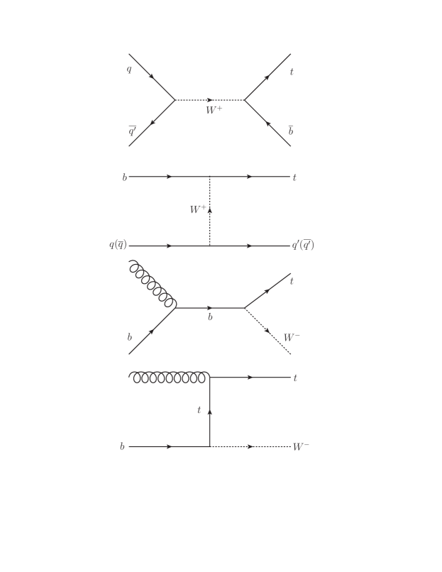
Figure 2: Tree-level Feynman diagrams for single-top production via the $s$ channel ($q\overline{q^{\prime}}\to t\overline{b}$), the $t$ channels ($bq\to tq^{\prime}$ and $b\overline{q}\to t\overline{q^{\prime}}$), and associated $t$-$W$ production ($bg\to tW^{-}$).

We are interested in the production and subsequent decay of a single top or antitop quark. Consider first the Lorentz- and CPT-invariant scenario in the usual SM. In parallel with the treatment of pair production in Sec. III.1 using the narrow-width approximation, the production and decay processes for a single top or antitop quark can be viewed as contributing distinct factors to the squared modulus of the matrix element. The decay factor is independent of the production mechanism, and examples of its form are given by the expressions (19) and (20). On the production side, four basic processes contribute to the tree-level amplitude for single-top production: $q\overline{q}$ annihilation via $W$ in the $s$ channel schan , $bq$ and $b\overline{q}$ weak interactions in the $t$ channel tchan , and $b$-gluon production of $tW$ wchan . In each case, the production factor is the squared matrix element for the process. The tree-level diagrams contributing to these processes are shown in Fig. 2.

Averaging over color and spin in the initial state and summing over color and spin in the final state, the squared matrix element for single-top production in $q\overline{q}$ annihilation via $W^{+}$ in the $s$ channel is given by

$$\overline{\sum}|{\cal M}_{q\overline{q}}|^{2}={\textstyle{{1}\over{4}}}{g^{4}}|V_{tb}|^{2}|V_{qq^{\prime}}|^{2}{{u(u-m_{t}^{2})}\over{(s-m_{W}^{2})^{2}}}.$$ (39)

In this expression, $V_{tb}$ and $V_{qq^{\prime}}$ are elements of the CKM matrix, $m_{t}$ is the mass of the top quark, $m_{W}$ is the mass of the $W^{+}$ boson, and the Mandelstam variables $s$, $t$, $u$ are given by

$$s=(p_{1}+p_{2})^{2}=(p_{3}+p_{4})^{2},$$

$$t=(p_{2}-p_{4})^{2}=(p_{1}-p_{3})^{2},$$

$$u=(p_{1}-p_{4})^{2}=(p_{2}-p_{3})^{2},$$ (40)

with $1,2,3,4=\overline{q^{\prime}},q,\overline{b},t$. Contributions to Eq. (39) from CKM-suppressed processes can also occur but are disregarded here for simplicity.

For single-top production via $bq$ weak interaction in the $t$ channel, the Lorentz-invariant squared matrix element is found to be

$$\overline{\sum}|{\cal M}_{bq}|^{2}={\textstyle{{1}\over{4}}}{g^{4}}|V_{tb}|^{2}|V_{qq^{\prime}}|^{2}{{s(s-m_{t}^{2})}\over{(t-m_{W}^{2})^{2}}},$$ (41)

where the Mandelstam variables (40) are defined with $1,2,3,4=q,b,q^{\prime},t$. The analogous result for single-top production via $b\overline{q}$ weak interaction in the $t$ channel is

$$\overline{\sum}|{\cal M}_{b\overline{q}}|^{2}={\textstyle{{1}\over{4}}}{g^{4}}|V_{tb}|^{2}|V_{qq^{\prime}}|^{2}{{u(u-m_{t}^{2})}\over{(t-m_{W}^{2})^{2}}},$$ (42)

where now $1,2,3,4=\overline{q},b,\overline{q^{\prime}},t$.

The fourth process, $bg$ associated production of $tW$, acquires contributions from the last two diagrams in Fig. 2. Including interference terms between the two diagrams, the squared matrix element is given in the SM by

$$\overline{\sum}|{{\cal M}_{bg}}|^{2} = \dfrac{g^{2}g_{\rm s}^{2}}{24}|V_{tb}|^{2}\bigg{\{}-\dfrac{2m_{t}^{2}}{m_{W}^{2}}-\bigg{(}\dfrac{m_{t}^{2}}{m_{W}^{2}}+2\bigg{)}$$

$$\hskip-35.0pt\times\bigg{[}\dfrac{s}{t-m_{t}^{2}}+\dfrac{m_{t}^{2}-2m_{W}^{2}+t}{s}$$

$$\hskip-25.0pt+\dfrac{2(m_{t}^{2}-m_{W}^{2})}{t-m_{t}^{2}}\bigg{(}\dfrac{m_{t}^{2}}{t-m_{t}^{2}}+\dfrac{m_{t}^{2}-m_{W}^{2}}{s}+1\bigg{)}\bigg{]}\bigg{\}},$$

where the Mandelstam variables (40) are defined using $1,2,3,4=b,g,W,t$.

The situation for single-antitop production can be studied in a similar way. The relevant diagrams for the available tree-level processes can be obtained by changing the charges on the $W$ bosons and reversing the direction of all the fermion lines in Fig. 2. The resulting squared matrix elements have the same forms as those given above, reflecting the CPT invariance of the SM.

At LHC energies, the cross section for single-top production in the $s$ channel is several times smaller than that for the $tW$ mode and more than an order of magnitude smaller than the dominant $t$ channels wb . Note that at the LHC the SM cross sections for the $tW$ and the $\overline{t}W$ modes are equal by CPT invariance. However, the cross section for single-$t$ production in either the $s$ or the $t$ channels is larger than that for single-$\overline{t}$ production because the LHC is a proton-proton collider. The CPT transformation in these channels relates results for the LHC to those for a hypothetical ‘anti-LHC’ involving antiprotons colliding with antiprotons.

The $s$-channel has features similar to the quark-annihilation $s$-channel calculation for $t$-$\overline{t}$ production. However, calculation of the cross sections for the $t$ channels and $tW$ mode faces a technical obstacle. The $b$ quark involved in these channels arises as part of the quark-gluon sea of the colliding proton, so even in the SM the diagrams shown in Fig. 2 are insufficient to yield accurate predictions for the cross sections. The $b$ quark can be viewed as emerging from $g\to b\overline{b}$ pair production in the sea, so in effect the $t$ channel involves $gq\to tq^{\prime}\overline{b}$ while the $tW$ mode involves $gg\to tW^{-}\overline{b}$. In these processes, when the $b$ quark moves collinear to its parent gluon, a divergence appears that is regulated by the $b$-quark mass. The effective perturbation expansion then contains large logarithms involving $\alpha_{\rm QCD}\ln(m_{W}/m_{b})$ and $\alpha_{\rm QCD}\ln(m_{t}/m_{b})$ instead of the usual $\alpha_{\rm QCD}$, so standard perturbation theory is unreliable. Instead, the $b$ quark must be handled via a parton distribution function obtained from perturbative QCD using gluons and parton distribution functions for the light quarks acot . Evolving the parton distribution function for the $b$-quark using the Altarelli-Parisi equation sums the large logarithms and enables calculation of the cross sections for these channels.

IV.2 CPT-violating case

Since single-top and $t$-$\overline{t}$ production involve distinct processes, it is reasonable to expect that studying the former would provide access to additional SME coefficients. In particular, as the results of Sec. III show that CPT violation is inaccessible in $t$-$\overline{t}$ production, single-top processes are of substantial potential interest for studies of CPT symmetry in the top-quark sector.

To investigate this possibility in a direct and comparatively simple way, we can restrict the SME Lagrange density for the top quark presented in Sec. II.1 to the special case where all coefficients for Lorentz violation are set to zero except those controlling CPT violation in the top-quark sector. Adopting the field redefinitions leading to Eq. (9), this corresponds to allowing only CPT violation involving the right-handed top quark, with the sole nonzero coefficient then being the coefficient $b_{\mu}$ introduced in Eq. (4). In this simplified model, all leading-order CPT-even Lorentz violation is absent. Also, CPT-violating effects are limited to right-handed contributions to the $t$ propagator.

Paralleling the CPT-invariant case described in Sec. IV.1, the squared modulus $|{\cal M}|^{2}$ of the amplitude can be written in the narrow-width approximation as the product of a production factor and a decay factor. The decay factor is comparatively straightforward to handle within the above scenario, since the only possible effect on the decay Feynman diagrams arises from a right-handed insertion on the initial $t$ propagator. However, direct calculation reveals that the CPT-violating contribution to the squared matrix element vanishes, in analogy with the zero contribution from $H_{\mu\nu}$ discussed in Sec. III.2. The decay factor for single-top production is therefore independent of CPT violation and can be taken to have a conventional form.

Determining the contributions to the production factor requires more effort. Within the above assumptions, the CPT-violating processes in the tree-level Feynman diagrams for single-top production involve right-handed insertions on the $t$ propagators in the diagrams shown in Fig. 2. At leading order, only one insertion is allowed at a time, yielding a total of five diagrams to consider. The corrections to the corresponding matrix element at leading order therefore involve the interference terms between these five diagrams and the Lorentz-invariant ones in Fig. 2. For example, the two Lorentz-invariant diagrams for the $tW$ mode are supplemented with three CPT-violating diagrams, each having an insertion on a $t$-quark line, so the corrections to the matrix element for this process contain six terms at leading order.

Several calculational simplifications emerge in the evaluation of the various contributions to the production matrix elements. Note first that in all diagrams for production the $t$ propagators are connected to a left-handed weak flavor-changing vertex. This means the right-handed $t$-quark insertions are partially cancelled by the projections, which reduces the complexity of some calculations. Another factor of relevance for simplifications is the ratio $m_{b}/m_{t}\simeq 1/40$, which means it is reasonable to neglect the $b$-quark mass in the calculations.

One complication appearing in the calculation of the squared matrix element is the determination of the spin sums over the top-quark states. The presence of CPT violation modifies these sums compared to the results for a conventional Dirac spinor. For the scenario of interest here, we find

$$\sum\limits_{\alpha=1,2}{u^{(\alpha)}\overline{u}^{(\alpha)}} = \not{p}+m_{t}+\not{b}-{{p\cdot b}\over{m_{t}^{2}}}(1+\gamma_{5})\not{p},$$

$$\sum\limits_{\alpha=1,2}{v^{(\alpha)}\overline{v}^{(\alpha)}} = \not{p}-m_{t}-\not{b}+{{p\cdot b}\over{m_{t}^{2}}}(1+\gamma_{5})\not{p},$$ (44)

where $u^{(\alpha)}(p)$ and $v^{(\alpha)}(p)$ are the eigenspinors of the modified Dirac equation. The derivation of this result is outlined in Appendix A.

With the above considerations, the calculation of the leading-order CPT-violating corrections to the squared matrix elements for the various single-top production processes can proceed in a straightforward manner. After some calculation, we find that the correction to the squared matrix element for single-top production in $q\overline{q}$ annihilation via $W^{+}$ in the $s$ channel takes the form

$$\delta\overline{\sum}|{\cal M}_{q\overline{q}}|^{2}=-{\textstyle{{1}\over{4}}}{g^{4}}|V_{tb}|^{2}|V_{qq^{\prime}}|^{2}{{2b\cdot p_{1}}\over{(s-m_{W}^{2})^{2}}},$$ (45)

where the Mandelstam variables (40) are defined with $1,2,3,4=\overline{q^{\prime}},q,\overline{b},t$ and contributions from CKM-suppressed analogues are disregarded as before. To obtain this result, we have averaged over color and spin in the initial state and summed over color and spin in the final state, as in the CPT-invariant case.

Similar calculations for single-top production via $bq$ and via $b\overline{q}$ weak interactions in the $t$ channel reveal that the corresponding CPT-violating corrections to the squared matrix elements are

$$\delta\overline{\sum}|{\cal M}_{bq}|^{2}={\textstyle{{1}\over{4}}}{g^{4}}|V_{tb}|^{2}|V_{qq^{\prime}}|^{2}{{2b\cdot p_{3}}\over{(t-m_{W}^{2})^{2}}},$$ (46)

where $1,2,3,4=q,b,q^{\prime},t$, and

$$\delta\overline{\sum}|{\cal M}_{b\overline{q}}|^{2}=-{\textstyle{{1}\over{4}}}{g^{4}}|V_{tb}|^{2}|V_{qq^{\prime}}|^{2}{{2b\cdot p_{1}}\over{(t-m_{W}^{2})^{2}}},$$ (47)

where $1,2,3,4=\overline{q},b,\overline{q^{\prime}},t$.

Finally, we can obtain the leading-order CPT-violating correction to $bg$ associated production of $tW$, which as mentioned above arises from the interference of three CPT-violating amplitudes with two Lorentz-invariant ones. The correction to the squared matrix element in this case is given by

$$\delta\overline{\sum}|{{\cal M}_{bg}}|^{2} = -{{g^{2}g_{\rm s}^{2}}\over{12}}|V_{tb}|^{2}b\cdot\bigg{\{}{{1}\over{m_{W}^{2}s}}\big{[}p_{2}(m_{t}^{2}-2m_{W}^{2})+p_{3}m_{t}^{2}+p_{4}t\big{]}+{{8m_{t}^{4}}\over{(t-m_{t}^{2})^{3}}}\bigg{(}{{m_{t}^{2}}\over{m_{W}^{2}}}p_{3}-p_{3}-p_{1}\bigg{)}$$ (48)

$$+{{1}\over{m_{W}^{2}s(t-m_{t}^{2})}}\big{[}p_{1}(2m_{t}^{4}-4m_{W}^{4}-m_{t}^{2}s)+p_{2}(3m_{t}^{4}-5m_{t}^{2}m_{W}^{2})$$

$$\hskip 100.0pt+(s+m_{t}^{2}-m_{W}^{2})(4m_{t}^{2}p_{3}-sp_{4})+m_{W}^{2}s(2p_{3}+p_{4})\big{]}$$

$$+{{m_{t}^{2}}\over{(t-m_{t}^{2})^{2}}}\bigg{[}p_{1}\bigg{(}{{3m_{t}^{2}}\over{m_{W}^{2}}}-3\bigg{)}+2p_{2}\bigg{(}{{m_{t}^{4}}\over{m_{W}^{2}s}}-{{m_{t}^{2}}\over{s}}+{{s}\over{m_{W}^{2}}}-{{m_{W}^{2}}\over{m_{t}^{2}}}\bigg{)}$$

$$+p_{3}\bigg{(}{{4m_{t}^{4}}\over{m_{W}^{2}s}}+{{8m_{W}^{2}-12m_{t}^{2}}\over{s}}+{{9m_{t}^{2}}\over{m_{W}^{2}}}-13\bigg{)}+p_{4}\bigg{(}{{4m_{W}^{2}-4m_{t}^{2}}\over{s}}-{{m_{t}^{2}+3s}\over{m_{W}^{2}}}+{{2s}\over{m_{t}^{2}}}-5\bigg{)}\bigg{]}\bigg{\}},$$

where now $1,2,3,4=b,g,W,t$.

The results for single-antitop production can be obtained in an analogous manner. The Feynman diagrams for the corresponding processes can be obtained by changing the charges on the $W$ bosons, reversing the direction of all the fermion lines in Fig. 2, and inserting the CPT-violating factor on the various $\overline{t}$ propagators in turn. Since the insertion involves a factor of $-b_{\mu}$, and since the leading-order contributions to the squared matrix elements arise through interference with the CPT-invariant SM diagrams, the corrections for single-antitop production are the negatives of those for single-top production given in Eqs. (45)-(48).

According to the discussion in Sec. II.3, the CPT-violating cross section for each process leading to single-top or single-antitop production exhibits sidereal variations that can in principle be used to extract constraints on components of the coefficient $b_{\mu}$ for CPT violation. At the LHC, the cross sections for single-top production in any one of the $s$ or $t$ channels is different from that for single-antitop production in the same channel because the LHC is a proton-proton collider and the light-quark content of the system changes under CPT. However, since the $tW^{-}$ and $\overline{t}W^{+}$ modes arise from $b$ and $\overline{b}$ quarks that in the SM are equally represented in the sea, the cross sections for the $tW^{-}$ and $\overline{t}W^{+}$ modes are equal in the SM. As a consequence, a comparison of the two cross sections via an asymmetry ${\cal A}_{\rm CPT}$ of the form (11) provides a distinct type of sensitivity to CPT violation. This asymmetry has both a time-independent piece and a sidereally varying piece, so careful study of its properties can provide information about the components $b_{Z}$ and $b_{T}$ that cannot readily be accessed via sidereal studies of any single process alone.

We remark in passing that all the production processes involve the weak interactions, and hence the single top or antitop quarks can be expected to emerge with a strong degree of polarization. An experimental analysis taking this into account might in principle achieve an enhanced sensitivity to CPT violation. However, we have shown above that interesting signals are already present in the comparatively simple spin-summed production rates. These therefore suffice to obtain a first measurement of the coefficient $b_{\mu}$ for CPT violation using the expected LHC statistics.

In a more general analysis using all the CPT-violating terms in Eq. (9), additional contributions from right-handed insertions on the $b$-quark propagators could also be included in the calculations. Most of the extra corrections arise in a straightforward way, generating numerous additional interference terms in the squared modulus of the matrix element. One additional complication arises in this more general case because any incoming $b$ quark in the production diagrams arises from the gluon sea via pair production. It is plausible a priori that including Lorentz and CPT violation in the $b$ sector affects the parton distribution function for the $b$ quark, which could require determining the CPT-violating corrections to the Altarelli-Parisi equation. Note, however, that at leading order the CPT-violating contributions to the $g\to b\overline{b}$ vertex appear in equal and opposite pairs because for every CPT-odd insertion associated with the $b$ line there is an equal and opposite contribution associated with the $\overline{b}$ line. This effect leads to cancellations in contributions from the quark-gluon sea of neutral mesons in the context of CPT violation in meson oscillations aksidereal . It suggests, for example, that in a narrow-width approximation for the $b$ production from the sea it may suffice for some data analyses to use the Lorentz-invariant parton distribution function for the $b$ quark in evaluating the CPT-violating contribution to the amplitude for the $tW$ channel. A detailed investigation of this intriguing issue lies outside our present scope but would be of definite interest for future work.

V Summary and Discussion

In this work, we investigated the prospects for tests of Lorentz and CPT invariance in the top-quark sector. The basic theory is introduced in Sec. II. Relevant terms involving the top-quark field are extracted from the general SME framework describing Lorentz and CPT violation using effective field theory and are presented in Eqs. (7) and (8). The issue of field and coordinate redefinitions is addressed in Sec. II.2, and a convenient choice limiting CPT violation to right-handed fields is presented in Eq. (9). Prospective signals to be sought are discussed in Sec. II.3, including both sidereal variations for Lorentz and CPT violation and asymmetries for CPT-violating rates.

The main results relevant to Lorentz violation in $t$-$\overline{t}$ pair production and decay are discussed in Sec. III. Both pair production by quark fusion and by gluon fusion are considered. The squared modulus of the matrix element for each case in the Lorentz-invariant limit is presented explicitly in the narrow-width approximation, where it factors according to Eq. (12). In Sec. III.2, CPT symmetry is shown to be preserved in $t$-$\overline{t}$ production and decay under the theoretical assumptions adopted in this work. The Lorentz-violating contributions to the squared modulus of the matrix element takes the form (22). The Lorentz-violating corrections due to production via quark fusion are presented in Sec. III.2.1, while those for gluon fusion can be found in Sec. III.2.2. The contributions on the decay side are obtained in Sec. III.2.3.

The issue of how to study CPT symmetry in the top-quark sector is addressed in Sec. IV. We show that single-top and antitop production offers interesting prospects to search for CPT violation, and we identify a limiting model for which calculations of the matrix element are simplified. Comments on the Lorentz-invariant case are provided in Sec. III.1, while the contributions to CPT violation for the various processes for single-top and single-antitop production are derived in Sec. IV.2.

Overall, the prospects appear good for studying Lorentz and CPT symmetry with the top quark. Already the D0 Collaboration has achieved a sensitivity of about 10% to components of the dimensionless SME coefficients $(c_{L})_{\mu\nu}$ and $(c_{R})_{\mu\nu}$ for CPT-even Lorentz violation, using a sidereal analysis of data from the Fermilab Tevatron. Our derivation of the matrix element for $t$-$\overline{t}$ production via gluon fusion given in Sec. III.2.2 now opens the door to a similar analysis at the LHC. Since the number of $t$-$\overline{t}$ pairs produced at the LHC is about an order of magnitude greater than that at the Tevatron, the attainable sensitivity to components of $(c_{L})_{\mu\nu}$ and $(c_{R})_{\mu\nu}$ can be expected to be of the order of a few percent.

Our proposed methodology for studying CPT symmetry via single-top production, described in Sec. IV.2, suggests access to the CPT-odd coefficient $b_{\mu}$ for the top quark via the LHC dataset now lies within reach for the first time. Since the statistical power in $t$-$\overline{t}$ production is around double that for single-top or antitop production, it is plausible that the observer-invariant dimensionless ratio $b_{\mu}p^{\mu}/s$ could be measured to around 5%. The relevant energy scale is set by the energy of the initial particles in the production process. These considerations suggest that the coefficient $b_{\mu}$, which has dimensions of mass, could be measured at a precision of order 100 GeV. A sidereal study would provide access to the components $b_{X}$ and $b_{Y}$ in the Sun-centered frame, while a comparison of single-top events with single-antitop events would give access to $b_{T}$ and $b_{Z}$.

The above crude estimate reveals that CPT violation in the top sector on a scale comparable to the $t$-quark mass remains a realistic experimental possibility. Comparatively large but experimentally viable Lorentz violation, known as countershaded Lorentz violation kt , is typically linked to weaker interactions that make it challenging to detect. Countershading is of theoretical interest in the context of the Lorentz hierarchy problem ksp because it has the potential to associate the scale of Lorentz violation to SM scales instead of ones suppressed by a power of the ratio of the weak scale to the Planck scale. Countershaded models include, for example, ones with Lorentz violation that appears only in matter-gravity couplings kt or in the pure-gravity sector bkx and hence is hidden by the comparatively feeble nature of the gravitational interaction, and ones in the neutrino sector involving oscillation-free Lorentz and CPT violation dkl that is hidden by the weak neutrino interactions.

For the top quark, the existence of countershaded CPT violation remains experimentally plausible due to the intrinsic difficulty of measuring properties of the top quark via single-top and single-antitop production, which in turn is a consequence of the weak interactions involved. Whether this scenario is realized in nature remains to be determined, but in any case it is evident that the top quark offers an intriguing open arena for future exploration of foundational properties of quantum field theory and the SM, including in particular Lorentz and CPT symmetry.

Appendix A Modified spin sums

In this appendix, we outline the derivation of the modified spin sums used in Sec. IV.2 in the derivation of the squared matrix elements for single-top production in the presence of CPT violation. The relevant terms in the Lagrange density are given by Eq. (9) with $(a_{L})_{\mu}$ set to zero, so all the CPT violation is controlled by the coefficient $b_{\mu}$. Leading-order solutions to the resulting modified Dirac equation can be obtained from the equations in Appendix A of the first paper in Ref. ck via the substitution $a_{\mu}\to-b_{\mu}$.

The spin sum can be readily calculated in the zero-momentum frame $S^{\prime}$. In what follows, variables with primes denote quantities in this frame. The spinors $u^{(\alpha)}(\vec{p}=0)$ and $v^{(\alpha)}(\vec{p}=0)$ have eigenenergies given to second order in Lorentz violation by

$$E^{(\alpha)\prime}_{u} = m_{t}+(-1)^{\alpha}|\vec{b^{\prime}}|-b^{\prime}_{0}+{{1}\over{2m_{t}}}\big{[}b^{\prime}_{0}-(-1)^{\alpha}|\vec{b^{\prime}}|\big{]}^{2},$$

$$E^{(\alpha)\prime}_{v} = E^{(\alpha)\prime}_{u}\big{|}_{b^{\prime}_{0}\to-b^{\prime}_{0}}.$$

The explicit forms of $u^{(\alpha)}(\vec{p}=0)$ and $v^{(\alpha)}(\vec{p}=0)$ at leading order in Lorentz violation are

$$u^{(\alpha)}(\vec{p}=0) = N_{u}^{(\alpha)}\left(\begin{array}[]{c}\phi_{u}^{(\alpha)}\\ X_{u}^{(\alpha)}\phi_{u}^{(\alpha)}\end{array}\right),$$ (52)

$$v^{(\alpha)}(\vec{p}=0) = N_{v}^{(\alpha)}\left(\begin{array}[]{c}X_{v}^{(\alpha)}\phi_{v}^{(\alpha)}\\ \phi_{v}^{(\alpha)}\end{array}\right).$$ (55)

In these expressions, the two-component spinors $\phi_{u,v}^{(\alpha)}$ take the form

$$\phi_{u,v}^{(\alpha)}=(\vec{\kappa}_{u,v}^{(\alpha)}\cdot\vec{\sigma}+\eta_{u,v}^{(\alpha)})\left(\begin{array}[]{c}0\\ 1\end{array}\right),$$ (56)

with

$${\vec{\kappa}}_{u}^{(\alpha)} = -4m_{t}\vec{b^{\prime}}\big{[}m_{t}-b^{\prime}_{0}+(-1)^{\alpha}|\vec{b^{\prime}}|\big{]},$$

$${\vec{\kappa}}_{v}^{(\alpha)} = -{\vec{\kappa}}_{u}^{(\alpha)}\big{|}_{b^{\prime}_{0}\to-b^{\prime}_{0}},$$

$$\eta_{u,v}^{(\alpha)} = -(-1)^{\alpha}|{\vec{\kappa}}_{u,v}^{(\alpha)}|,$$ (57)

where we have assumed that the components of $b^{\prime}_{\mu}$ are all smaller than $m_{t}$. Also, the matrices $X_{u,v}^{(\alpha)}$ in Eq. (55) are given by

$$X_{u}^{(\alpha)}=-X_{v}^{(\alpha)}={{1}\over{2m_{t}}}(\vec{b^{\prime}}\cdot\vec{\sigma}-b^{\prime}_{0}).$$ (58)

For the solutions (55), we adopt the normalization conditions

$$\overline{u}^{(\alpha)}u^{(\alpha)}=-\overline{v}^{(\alpha)}v^{(\alpha)}=2m_{t},$$ (59)

which imply

$$|N_{u,v}^{(\alpha)}|^{2}=\dfrac{2m_{t}}{\phi_{u,v}^{(\alpha)\dagger}\phi_{u,v}^{(\alpha)}}$$ (60)

at leading order.

Using the above results to evaluate the spin sums in the frame $S^{\prime}$ yields

$$\sum\limits_{\alpha=1,2}u^{(\alpha)}\overline{u}^{(\alpha)} = \left(\begin{array}[]{cc}2m_{t}&b^{\prime}_{0}-\vec{b^{\prime}}\cdot\vec{\sigma}\\ -b^{\prime}_{0}+\vec{b^{\prime}}\cdot\vec{\sigma}&0\end{array}\right),$$ (63)

$$\sum\limits_{\alpha=1,2}v^{(\alpha)}\overline{v}^{(\alpha)} = \left(\begin{array}[]{cc}0&-b^{\prime}_{0}+\vec{b^{\prime}}\cdot\vec{\sigma}\\ b^{\prime}_{0}-\vec{b^{\prime}}\cdot\vec{\sigma}&-2m_{t}\end{array}\right).\qquad$$ (66)

Unlike the Lorentz-invariant case, the difference of these two results is no longer proportional to the identity matrix, although each of the two spin sums still acts as a projection operator on its own subspace. However, the completeness relation between the two subspaces is guaranteed to hold only for the original hamiltonian, prior to the reinterpretation of negative-energy states. The CPT-violating shifts reflected in the eigenenergies (LABEL:eigenen) introduce nonorthogonal behavior of the two subspaces upon reinterpretation ck .

To obtain results valid for the frame $S$ in which the spinors have nonzero momentum $\vec{p}$, we can perform an observer Lorentz transformation. For rapidity $\vec{\zeta}$ in $S$, the boost takes the form

$$u^{(\alpha)}=Su^{\prime(\alpha)},\quad v^{(\alpha)}=Sv^{\prime(\alpha)},\quad S=\exp(i\zeta^{j}\sigma^{0j}/2),\quad$$ (67)

where as usual $\sigma^{0j}=i[\gamma^{0},\gamma^{j}]/2$. Under the observer transformation, the coefficients $b^{\prime}_{\mu}$ are related to those in the frame $S$ by

$$b^{\prime}_{0}=\gamma(b_{0}-\vec{v}\cdot\vec{b}),\quad\vec{b^{\prime}}=\vec{b}+\dfrac{\gamma-1}{v^{2}}(\vec{v}\cdot\vec{b})\vec{v}-\gamma b_{0}\vec{v},\quad$$ (68)

where $\vec{v}$ is the velocity of the particle in $S$ and $\gamma=1/{\sqrt{1-\vec{v}^{2}}}$, as usual. Note that the relationship between $\vec{p}$ and $\vec{v}$ acquires corrections involving the coefficients for Lorentz violation ck , but at leading order this has no effect on the present derivation. Note also that the transformations of the spinors and of the coefficients commute. Implementing these calculations leads to the modified spin sums (44), which hold in the frame $S$.

References

- (1) F. Abe et al., CDF Collaboration, Phys. Rev. Lett. 74, 2626 (1995); S. Abachi et al., D0 Collaboration, Phys. Rev. Lett. 74, 2422(1995).
- (2) For reviews of top-quark physics see, for example, W. Bernreuther, J. Phys. G 35, 083001 (2008); K. Lannon, F. Margaroli, and C. Neu, Eur. Phys. J. C 72, 2120 (2012); E. Boos, O. Brandt, D. Denisov, S. Denisov, and P. Grannis, arXiv:1509.03325.
- (3) V.A. Kostelecký and S. Samuel, Phys. Rev. D 39, 683 (1989); V.A. Kostelecký and R. Potting, Nucl. Phys. B 359, 545 (1991); Phys. Rev. D 51, 3923 (1995).
- (4) Data Tables for Lorentz and CPT Violation, 2015 edition, V.A. Kostelecký and N. Russell, arXiv:0801.0287v8.
- (5) V.M. Abazov et al., D0 Collaboration, Phys. Rev. Lett. 108, 261603 (2012).
- (6) V.A. Kostelecký, Phys. Rev. D 69, 105009 (2004).
- (7) R. Bluhm, Phys. Rev. D 91, 065034 (2015).
- (8) D. Colladay and V.A. Kostelecký, Phys. Rev. D 55, 6760 (1997); Phys. Rev. D 58, 116002 (1998).
- (9) O.W. Greenberg, Phys. Rev. Lett. 89, 231602 (2002).
- (10) For reviews see, for example, J.D. Tasson, Rept. Prog. Phys. 77, 062901 (2014); R. Bluhm, Lect. Notes Phys. 702, 191 (2006).
- (11) ATLAS Collaboration, Measurement of the Top Quark Mass from TeV ATLAS Data Using a 3-Dimensional Template Fit, ATLAS-CONF-2013-046, May 2013; S. Chatrchyan et al., CMS Collaboration, JHEP 1212, 105 (2012); T. Aaltonen et al., CDF Collaboration, Phys. Rev. Lett. 109, 152003 (2012); V.M. Abazov et al., D0 Collaboration, Phys. Rev. D 84, 032004 (2011).
- (12) G. Aad et al., ATLAS Collaboration, JHEP 1311, 031 (2013); S. Chatrchyan et al., CMS Collaboration, Constraints on the Top-Quark Charge from Top-Pair Events, CMS PAS TOP-11-031, March 2012; T. Aaltonen et al., CDF Collaboration, Phys. Rev. D 88, 032003 (2013); V.M. Abazov et al., D0 Collaboration, Phys. Rev. Lett. 98, 041801 (2007).
- (13) T. Aaltonen et al., CDF Collaboration, Phys. Rev. Lett. 111, 202001 (2013); V.M. Abazov et al., D0 Collaboration, Phys. Rev. D 85, 091104(R) (2012).
- (14) M. Cambiaso, R. Lehnert, and R. Potting, Phys. Rev. D 90, 065003 (2014); D. Colladay and V.A. Kostelecký, Phys. Lett. B 511, 209 (2001).
- (15) V.A. Kostelecký and M. Mewes, Phys. Rev. D 66, 056005 (2002).
- (16) D. Colladay and P. McDonald, J. Math. Phys. 43, 3554 (2002); Q.G. Bailey and V.A. Kostelecký, Phys. Rev. D 70, 076006 (2004); B. Altschul, J. Phys. A 39 13757 (2006); R. Lehnert, Phys. Rev. D 74, 125001 (2006); V.A. Kostelecký and N. Russell, Phys. Lett. B 693, 443 (2010) V.A. Kostelecký and J.D. Tasson, Phys. Rev. D 83, 016013 (2011); V.A. Kostelecký and M. Mewes, Phys. Rev. D 88, 096006 (2013).
- (17) V.A. Kostelecký and N. Russell, Phys. Lett. B 693, 443 (2010); V.A. Kostelecký, Phys. Lett. B 701, 137 (2011); D. Colladay and P. McDonald, Phys. Rev. D 85, 044042 (2012); V.A. Kostelecký, N. Russell, and R. Tso, Phys. Lett. B 716, 470 (2012); arXiv:1507.01018. J.E.G. Silva and C.A.S. Almeida, Phys. Lett. B 731, 74 (2014); M. Schreck, Phys. Rev. D 91, 105001 (2015); Eur. J. Phys. C 75, 187 (2015); arXiv:1508.00216; N. Russell, Phys. Rev. D 91, 045008 (2015); J. Foster and R. Lehnert, Phys. Lett. B 746, 164 (2015).
- (18) For reviews see, for example, J.R. Incandela, A. Quadt, W. Wagner, and D. Wicke, Prog. Part. Nucl. Phys. 63, 239 (2009); D. Chakraborty, J. Konigsberg, and D.L. Rainwater, Ann. Rev. Nucl. Part. Sci. 53, 301 (2003); T.M.P. Tait and C.-P. Yuan, Phys. Rev. D 63, 014018 (2000).
- (19) R. Bluhm, V.A. Kostelecký, C.D. Lane, and N. Russell, Phys. Rev. D 68, 125008 (2003); Phys. Rev. Lett. 88, 090801 (2002); V.A. Kostelecký and M. Mewes, Phys. Rev. D 66, 056005 (2002).
- (20) V.A. Kostelecký and R. Lehnert, Phys. Rev. D 63, 065008 (2001).
- (21) V.A. Kostelecký, Phys. Rev. Lett. 80, 1818 (1998).
- (22) V.A. Kostelecký, Phys. Rev. D 61, 016002 (1999); Phys. Rev. D 64, 076001 (2001); V.A. Kostelecký and R.J. Van Kooten, Phys. Rev. D 82, 101702(R) (2010).
- (23) H. Nguyen, KTeV Collaboration, hep-ex/0112046.
- (24) D. Babusci et al., KLOE Collaboration, Phys. Lett. B 730, 89 (2014).
- (25) J. Link et al., FOCUS Collaboration, Phys. Lett. B 556, 7 (2003).
- (26) B. Aubert et al., BaBar Collaboration, Phys. Rev. Lett. 100, 131802 (2008).
- (27) V.M. Abazov et al., D0 Collaboration, arXiv:1506.04123.
- (28) R. Kehoe, M. Narain, and A. Kumar, Int. J. Mod. Phys. A 23, 353 (2008).
- (29) H. Pilkuhn, The Interactions of Hadrons, North Holland, Amsterdam, 1967.
- (30) D. Berdine, N. Kauer, and D. Rainwater, Phys. Rev. Lett. 99, 111601 (2007).
- (31) C.F. Uhlemann and N. Kauer, Nucl. Phys. B 814, 195 (2009).
- (32) M. Gluck, J.F. Owens and E. Reya, Phys. Rev. D 17, 2324 (1978).
- (33) B.L. Combridge, Nucl. Phys. B 151, 429 (1979).
- (34) R.K. Ellis, W.J. Stirling and B.R. Webber, QCD and Collider Physics, Cambridge University Press, Cambridge, 2003.
- (35) R.P. Feynman, Acta Phys. Polon. 24, 697 (1963).
- (36) H.M. Georgi, S.L. Glashow, M.E. Machacek and D.V. Nanopoulos, Ann. Phys. 114, 273 (1978).
- (37) G. Mahlon and S. Parke, Phys. Lett. B 411, 173 (1997).
- (38) V.M. Abazov et al., D0 Collaboration, Phys. Rev. D 74, 092005 (2006).
- (39) V.M. Abazov et al., D0 Collaboration, Phys. Rev. Lett. 103, 092001 (2009); T. Aaltonen et al., CDF Collaboration, Phys. Rev. Lett. 103, 092002 (2009).
- (40) S. Cortese and R. Petronzio, Phys. Lett. B 253, 494 (1991); T. Stelzer and S. Willenbrock, Phys. Lett. B 357, 125 (1995).
- (41) S.S.D. Willenbrock and D.A. Dicus, Phys. Rev. D 34, 155 (1986); C.P. Yuan, Phys. Rev. D 41, 42 (1990); R.K. Ellis and S.J. Parke, Phys. Rev. D 46, 3785 (1992); D.O. Carlson and C.P. Yuan, Phys. Lett. B 306, 386 (1993).
- (42) S. Moretti, Phys. Rev. D 56, 7427 (1997); A.S. Belyaev, E.E. Boos, and L.V. Dudko, Phys. Rev. D 59, 075001 (1999); T.M.P. Tait, Phys. Rev. D 61, 034001 (1999); A. Belyaev and E. Boos, Phys. Rev. D 63, 034012 (2001).
- (43) M.A.G. Aivazis, J.C. Collins, F.I. Olness, and W.K. Tung, Phys. Rev. D 50, 3102 (1994).
- (44) V.A. Kostelecký and J.D. Tasson, Phys. Rev. Lett. 102, 010402 (2009).
- (45) Q.G. Bailey, V.A. Kostelecký, and R. Xu, Phys. Rev. D 91, 022006 (2015).
- (46) J.S. Díaz, V.A. Kostelecký, and R. Lehnert, Phys. Rev. D 88, 071902(R) (2013).