Vector-borne diseases models with residence times - a Lagrangian perspective

Derdei Bicharaa,b and Carlos Castillo-Chavezc
a Department of Mathematics, California State University, Fullerton,
b Center for Computational and Applied Mathematics,
800 N. State College Blvd, Fullerton, CA 92831.
c Simon A. Levin Mathematical, Computational and Modeling Science Center,
Arizona State University, Tempe, AZ 85287
E-mails: dbichara@fullerton.edu & ccchavez@asu.edu
Abstract

A multi-patch and multi-group modeling framework describing the dynamics of a class of diseases driven by the interactions between vectors and hosts structured by groups is formulated. Hosts’ dispersal is modeled in terms of patch-residence times with the nonlinear dynamics taking into account the effective patch-host size. The residence times basic reproduction number 0subscript0\mathcal{R}_{0} is computed and shown to depend on the relative environmental risk of infection. The model is robust, that is, the disease free equilibrium is globally asymptotically stable (GAS) if 01subscript01\mathcal{R}_{0}\leq 1 and a unique interior endemic equilibrium is shown to exist that is GAS whenever 0>1subscript01\mathcal{R}_{0}>1 whenever the configuration of host-vector interactions is irreducible. The effects of patchiness and groupness, a measure of host-vector heterogeneous structure, on the basic reproduction number 0subscript0\mathcal{R}_{0}, are explored. Numerical simulations are carried out to highlight the effects of residence times on disease prevalence.

Mathematics Subject Classification: 92D30, 34D23, 34A34, 34C12 .

Keywords:

Vector-borne diseases, Human dispersal, Basic reproduction number, Global stability, Nonlinear dynamical systems.

Introduction

Vector-borne diseases, a major public health problem around the world, are responsible for over one million death and hundreds of millions cases each year [55, 69] and so diminishing their impact is a worldwide priority. Travel, climate change and trade have significantly altered vector-borne diseases dynamics [10, 26, 41, 56, 57]. Sir Ronald Ross [60] was the first to model a vector borne disease dynamics. Ross’s paper [60] and follow up work [61, 62, 63] laid the foundation of what is known today as the field of mathematical or theoretical epidemiology. There is an extensive literature associated with the the study of vector-host interactions in the context of human diseases ([2, 4, 6, 14, 15, 16, 20, 21, 22, 23, 24, 33, 43, 45, 47, 48] and the references therein). Sparse theoretical results exist on the role of geographical heterogeneity on the spread of vector-borne diseases, mostly via metapopulation models [1, 3, 5, 18, 29, 70, 58, 65, 73], that assume that the movement of host is “permanent”; this approach has been referred as Eulerian [31, 52, 51]. A Lagrangian perspective considers the movement of individuals across patches in a framework where the hosts’ origin or identity are never lost. This approach, useful in the study of the role of movement of individuals in highly connected settings albeit it has received limited attention [18, 25, 36, 58, 64].

The concept of Langragian and Eulerian approaches were implemented by Okubo et al. [52, 51] in modeling the diffusion and aggregation of animal populations in ecology. This nomenclature has been used in the context of epidemic models by Cosner et al. [18]. The use of a Lagrangian approach in the study of the dynamics and control of vector-borne diseases has also been explored in [25, 33] prior this work. Specifically, Dye and Hasibeder [25, 33] considered the study of vector-born dynamics via SISSI𝑆𝐼𝑆𝑆𝐼SIS-SI type host-vector models in the context of n𝑛n patch systems. Rodriguez and Torres-Sorando [58] used a Lagrangian perspective via the incorporation of short-time visitations to multiple patches, also in the context of vector borne disease. In [64], authors also considered a patchy Ross-Macdonald model and derived patch specific basic reproduction number in order to identify which patch is a source or a sink. More recently, Iggidr et al. [36] introduced a general SIRSI𝑆𝐼𝑅𝑆𝐼SIR-SI multi group deriving necessary and sufficient conditions for the existence of a sharp threshold [36]. Their [36] abstract setting did not incorporate residence times explicitly, albeit their general infection terms technically may allow for their inclusion. The study in [36] and related papers, with the exception of [33, 25], assume that hosts and vectors are residents or members of particular patch or group. Our framework can handle multiple levels of organization including the host’s age or socio-economic structure (see [46, 68] for the age factors and [8, 39, 53] for the socio-economics’ role). Since vector transmission is often determined by the vectors’ place of residence, it is often useful to decouple the host’s structure from that of vectors’ population whenever possible.

In this paper, we consider a vector-host model where the host population is structured by groups/classes that interact with non-mobile vectors living in multiple patches/environments. The hosts’ groups may be defined by socioeconomic background, gender, or age. The vectors’ patches represent the vectors’ “space”, which include schools, farms, workplaces etc. Hosts, in general, will distribute their time in a multitude of vectors’ places of residence (patches). In our setup, we assume that the spatial scale under consideration is such that ignoring vector mobility across patches is acceptable. There are evidences that such an assumption is reasonable, for example, Dengue and Chikungunya’s urban vectors Aedes aegypti rarely travel more than a few tens of meters during their lifespan [1, 54]; the mainly rural but urban adapted vector Aedes albopictus have maximum dispersal of 400-600 meters [35, 49]; according to [9, 49], the vectors Aedes albopictus are unlikely to travel long distance due to wind speed variability, in fact, they exhibit a tendency to fly closer to the ground, desisting to fly during heavy winds; the adult Anopheles( vector of malaria) does not fly more than 2 kilometers [67]; and, Anopheles gambiae’s (the main malaria vector in Africa) maximal flight distance is 10 kilometer [38]. In short, the spread of vector-borne diseases, in many instances, is primarily due to hosts’ dispersal. Therefore, it is assumed here as in [5, 73] that vectors do not abandon their geographical environment or patch. There are alternative modes of mosquitoes dispersal like those generated by trade, including the used-tires’ trade [50, 59].

The host population is structured into n𝑛n groups with dispersal modeled via the residence times matrix =(pij)1in,1jmsubscriptsubscript𝑝𝑖𝑗1𝑖𝑛1𝑗𝑚\mathbb{P}=(p_{ij})_{\begin{subarray}{c}1\leq i\leq n,\\ 1\leq j\leq m\end{subarray}}, where pijsubscript𝑝𝑖𝑗p_{ij} denotes the proportion of time that a host member of Groups i𝑖i spends in Patch j𝑗j. The use of this approach impacts the temporal dynamics of the effective host population size in each patch. Host effective population size per patch, that is the number of hosts of each group at time t𝑡t in Patch j𝑗j, j=1,2,,m𝑗12𝑚j=1,2,\dots,m; is computed using the entries of the matrix \mathbb{P} as weights. The density of effective infected host per patch account for both effective population and effective infected population size in each patch.

The host effective population size has not been incorporated in the literature using a Lagrangian approach in the contet of vector-borne diseases before [18, 58] (but see [11]). Our formulation generalize the case where vectors and hosts are defined by jointly inhabited patches [18, 36, 58]. We prove that the disease free equilibrium is GAS if 01subscript01\mathcal{R}_{0}\leq 1 and that a unique endemic equilibrium exists and is GAS if 0>1subscript01\mathcal{R}_{0}>1 whenever the multi-patch, multi-group system is irreducible. This approach has been used in the study of a general SIS𝑆𝐼𝑆SIS model in the context of communicable diseases ([7]).

The paper is organized as follow. Section 1 is devoted to the derivation and basic properties of the model; Section 2 deals with the stability analysis of the disease free equilibrium (DFE) and the endemic equilibrium. Section 3, highlights the role of heterogeneity in term of patch and group variability on the basic reproduction number; Section 4 highlights tour results in the context of 2 groups, 2 patches and 2 groups and 3 patches via simulations. Section 5 collects our conclusions and thoughts on the usefulness of this approach and list possible extensions.

1 Derivation of the model

We consider the dynamics of human-vector interactions within a population composed of n𝑛n social groups and m𝑚m environments or patches. We denote by Nh,isubscript𝑁𝑖N_{h,i} the host population in social group i𝑖i, i=1,,i𝑖1𝑖i=1,\dots,i, and Nv,jsubscript𝑁𝑣𝑗N_{v,j} vector population in Patch j𝑗j, j=1,,m𝑗1𝑚j=1,\dots,m. The susceptible and infected host populations in group i𝑖i, i=1,,n𝑖1𝑛i=1,\dots,n , at time t𝑡t, are denoted by Sh,i(t)subscript𝑆𝑖𝑡S_{h,i}(t) and Ih,i(t)subscript𝐼𝑖𝑡I_{h,i}(t) respectively. It is assumed that the total host population in each group is constant, that is Nh,i=Sh,i(t)+Ih,i(t)subscript𝑁𝑖subscript𝑆𝑖𝑡subscript𝐼𝑖𝑡N_{h,i}=S_{h,i}(t)+I_{h,i}(t); that the disease in the host is captured by an SIS𝑆𝐼𝑆SIS epidemic model while the vectors’ dynamics follows an SI𝑆𝐼SI framework. The vector population in each patch is composed by Sv,jsubscript𝑆𝑣𝑗S_{v,j} and Iv,jsubscript𝐼𝑣𝑗I_{v,j}, the susceptible and infected vector populations in Patch j𝑗j, j=1,,m𝑗1𝑚j=1,\dots,m, respectively.

The entries of the residence times matrix \mathbb{P} denote the proportion of time that individuals of different groups spend in each patches; specifically pijsubscript𝑝𝑖𝑗p_{ij} represents the proportion of time that members of group i𝑖i spend in Patch j𝑗j (pij0subscript𝑝𝑖𝑗0p_{ij}\geq 0 for all j𝑗j and j=1mpij=1superscriptsubscript𝑗1𝑚subscript𝑝𝑖𝑗1\sum_{j=1}^{m}p_{ij}=1 for all i𝑖i). The susceptible individuals of group i𝑖i (Sh,isubscript𝑆𝑖S_{h,i}) are generated through birth at the per-capita rate μisubscript𝜇𝑖\mu_{i} and they recover from infection at the per-capita rate γisubscript𝛾𝑖\gamma_{i}. It is assumed that all offsprings are susceptible and that the disease does not confer immunity. The birth of susceptible individuals in group i𝑖i is compensated by deaths, maintaining constant host population size in each group. The host population is at risk of infection in every patches from its interaction with local infected vectors (Iv,j,j=1,,mformulae-sequencesubscript𝐼𝑣𝑗𝑗1𝑚I_{v,j},\;j=1,\dots,m). Hence, the dynamics of the the susceptible host of group i𝑖i, for i=1,,n𝑖1𝑛i=1,\dots,n, is given by:

S˙h,i=μiNh,i+γiIh,ij=1mbj(Nh,Nv,j)βv,hpijSh,iIv,jNv,jμiSh,isubscript˙𝑆𝑖subscript𝜇𝑖subscript𝑁𝑖subscript𝛾𝑖subscript𝐼𝑖superscriptsubscript𝑗1𝑚subscript𝑏𝑗subscript𝑁subscript𝑁𝑣𝑗subscript𝛽𝑣subscript𝑝𝑖𝑗subscript𝑆𝑖subscript𝐼𝑣𝑗subscript𝑁𝑣𝑗subscript𝜇𝑖subscript𝑆𝑖\dot{S}_{h,i}=\mu_{i}N_{h,i}+\gamma_{i}I_{h,i}-\sum_{j=1}^{m}b_{j}(N_{h},N_{v,j})\beta_{v,h}p_{ij}S_{h,i}\frac{I_{v,j}}{N_{v,j}}-\mu_{i}S_{h,i}

where bj(Nh,Nv,j)subscript𝑏𝑗subscript𝑁subscript𝑁𝑣𝑗b_{j}(N_{h},N_{v,j}) is the number of mosquito bites per human per unit of time [13, 15, 27, 30] in Patch j𝑗j. bj(Nh,Nv,j)subscript𝑏𝑗subscript𝑁subscript𝑁𝑣𝑗b_{j}(N_{h},N_{v,j}) is assumed to be a function of the number of host in Patch j𝑗j; a population that includes visitors from other patches.

The dynamics of infected hosts of group i𝑖i, i=1,,n𝑖1𝑛i=1,\dots,n, is modeled as follows

I˙h,i=j=1mbj(Nh,Nv,j)βvhpijSh,iIv,jNv,j(μi+γi)Ih,isubscript˙𝐼𝑖superscriptsubscript𝑗1𝑚subscript𝑏𝑗subscript𝑁subscript𝑁𝑣𝑗subscript𝛽𝑣subscript𝑝𝑖𝑗subscript𝑆𝑖subscript𝐼𝑣𝑗subscript𝑁𝑣𝑗subscript𝜇𝑖subscript𝛾𝑖subscript𝐼𝑖\dot{I}_{h,i}=\sum_{j=1}^{m}b_{j}(N_{h},N_{v,j})\beta_{vh}p_{ij}S_{h,i}\frac{I_{v,j}}{N_{v,j}}-(\mu_{i}+\gamma_{i})I_{h,i} (1)

The susceptible vectors in Patch j𝑗j are replenished via constant recruitment Λv,jsubscriptΛ𝑣𝑗\Lambda_{v,j}, subject to death at the per-capita rate μvsubscript𝜇𝑣\mu_{v} and removed (through harvesting and spraying) at the per-capita rate δjsubscript𝛿𝑗\delta_{j}. We suppose that the natural per-capita vectors’ death rates are the same in all patches. Though, the vectors do not move across patches, the susceptible mosquitoes in Patch j𝑗j (Sv,jsubscript𝑆𝑣𝑗S_{v,j}) may, of course, be infected by infected hosts of any group while visiting Patch j𝑗j. The effective proportion of infected individuals in Patch j𝑗j is therefore given by

i=1npijIh,ik=1npkjNh,ksuperscriptsubscript𝑖1𝑛subscript𝑝𝑖𝑗subscript𝐼𝑖superscriptsubscript𝑘1𝑛subscript𝑝𝑘𝑗subscript𝑁𝑘\frac{\sum_{i=1}^{n}p_{ij}I_{h,i}}{\sum_{k=1}^{n}p_{kj}N_{h,k}}

Hence, the dynamics of susceptible vector in Patch j𝑗j, j=1,,m𝑗1𝑚j=1,\dots,m in patch j𝑗j at time t𝑡t is given by

S˙v,j=Λv,iajβhvSv,ji=1npijIh,ik=1npkjNh,k(μv+δj)Sv,jsubscript˙𝑆𝑣𝑗subscriptΛ𝑣𝑖subscript𝑎𝑗subscript𝛽𝑣subscript𝑆𝑣𝑗superscriptsubscript𝑖1𝑛subscript𝑝𝑖𝑗subscript𝐼𝑖superscriptsubscript𝑘1𝑛subscript𝑝𝑘𝑗subscript𝑁𝑘subscript𝜇𝑣subscript𝛿𝑗subscript𝑆𝑣𝑗\dot{S}_{v,j}=\Lambda_{v,i}-a_{j}\beta_{hv}S_{v,j}\frac{\sum_{i=1}^{n}p_{ij}I_{h,i}}{\sum_{k=1}^{n}p_{kj}N_{h,k}}-(\mu_{v}+\delta_{j})S_{v,j}

where ajsubscript𝑎𝑗a_{j} is the number of bites per mosquito per unit of time in Patch j𝑗j, assumed to be constant.

The dynamics of infected vectors in Patch j𝑗j is given by

I˙v,j=ajβhvSv,ji=1npijIh,ik=1npkjNh,k(μv+δj)Iv,jsubscript˙𝐼𝑣𝑗subscript𝑎𝑗subscript𝛽𝑣subscript𝑆𝑣𝑗superscriptsubscript𝑖1𝑛subscript𝑝𝑖𝑗subscript𝐼𝑖superscriptsubscript𝑘1𝑛subscript𝑝𝑘𝑗subscript𝑁𝑘subscript𝜇𝑣subscript𝛿𝑗subscript𝐼𝑣𝑗\dot{I}_{v,j}=a_{j}\beta_{hv}S_{v,j}\frac{\sum_{i=1}^{n}p_{ij}I_{h,i}}{\sum_{k=1}^{n}p_{kj}N_{h,k}}-(\mu_{v}+\delta_{j})I_{v,j} (2)

We know that the total number of bites by mosquitoes (ajNv,jsubscript𝑎𝑗subscript𝑁𝑣𝑗a_{j}N_{v,j} in Patch j𝑗j) should equal the total number of bites received by humans (bj(Nh,Nv)k=1npkjNh,ksubscript𝑏𝑗subscript𝑁subscript𝑁𝑣superscriptsubscript𝑘1𝑛subscript𝑝𝑘𝑗subscript𝑁𝑘b_{j}(N_{h},N_{v})\sum_{k=1}^{n}p_{kj}N_{h,k}) [2, 13, 48]. In our case, this conservation of contact rates should be satisfied in each patch. Hence, for Patch j𝑗j, we have:

ajNv,j=bj(Nh,Nv,j)k=1npkjNh,k.subscript𝑎𝑗subscript𝑁𝑣𝑗subscript𝑏𝑗subscript𝑁subscript𝑁𝑣𝑗superscriptsubscript𝑘1𝑛subscript𝑝𝑘𝑗subscript𝑁𝑘a_{j}N_{v,j}=b_{j}(N_{h},N_{v,j})\sum_{k=1}^{n}p_{kj}N_{h,k}.

This implies that:

bj(Nh,Nv,j)=ajNv,jk=1npkjNh,ksubscript𝑏𝑗subscript𝑁subscript𝑁𝑣𝑗subscript𝑎𝑗subscript𝑁𝑣𝑗superscriptsubscript𝑘1𝑛subscript𝑝𝑘𝑗subscript𝑁𝑘b_{j}(N_{h},N_{v,j})=\frac{a_{j}N_{v,j}}{\sum_{k=1}^{n}p_{kj}N_{h,k}} (3)

Hence, the disease dynamics for n𝑛n host groups interacting in m𝑚m different environments subjected to resident vectors is completely described by the following system:

{S˙h,i=μiNh,i+γiIh,iβvhSh,ij=1majpijIv,jk=1npkjNh,kμiSh,iI˙h,i=βvhSh,ij=1majpijIv,jk=1npkjNh,k(μi+γi)Ih,iS˙v,j=Λv,jajβhvSv,ji=1npijIh,ik=1npkjNh,k(μv+δj)Sv,jI˙v,j=βhvSv,ji=1npijIh,ik=1npkjNh,k(μv+δj)Iv,j,casessubscript˙𝑆𝑖subscript𝜇𝑖subscript𝑁𝑖subscript𝛾𝑖subscript𝐼𝑖subscript𝛽𝑣subscript𝑆𝑖superscriptsubscript𝑗1𝑚subscript𝑎𝑗subscript𝑝𝑖𝑗subscript𝐼𝑣𝑗superscriptsubscript𝑘1𝑛subscript𝑝𝑘𝑗subscript𝑁𝑘subscript𝜇𝑖subscript𝑆𝑖missing-subexpressionmissing-subexpressionmissing-subexpressionmissing-subexpressionmissing-subexpressionmissing-subexpressionmissing-subexpressionsubscript˙𝐼𝑖subscript𝛽𝑣subscript𝑆𝑖superscriptsubscript𝑗1𝑚subscript𝑎𝑗subscript𝑝𝑖𝑗subscript𝐼𝑣𝑗superscriptsubscript𝑘1𝑛subscript𝑝𝑘𝑗subscript𝑁𝑘subscript𝜇𝑖subscript𝛾𝑖subscript𝐼𝑖missing-subexpressionmissing-subexpressionmissing-subexpressionmissing-subexpressionmissing-subexpressionmissing-subexpressionmissing-subexpressionsubscript˙𝑆𝑣𝑗subscriptΛ𝑣𝑗subscript𝑎𝑗subscript𝛽𝑣subscript𝑆𝑣𝑗superscriptsubscript𝑖1𝑛subscript𝑝𝑖𝑗subscript𝐼𝑖superscriptsubscript𝑘1𝑛subscript𝑝𝑘𝑗subscript𝑁𝑘subscript𝜇𝑣subscript𝛿𝑗subscript𝑆𝑣𝑗missing-subexpressionmissing-subexpressionmissing-subexpressionmissing-subexpressionmissing-subexpressionmissing-subexpressionmissing-subexpressionsubscript˙𝐼𝑣𝑗subscript𝛽𝑣subscript𝑆𝑣𝑗superscriptsubscript𝑖1𝑛subscript𝑝𝑖𝑗subscript𝐼𝑖superscriptsubscript𝑘1𝑛subscript𝑝𝑘𝑗subscript𝑁𝑘subscript𝜇𝑣subscript𝛿𝑗subscript𝐼𝑣𝑗missing-subexpressionmissing-subexpressionmissing-subexpression\left\{\begin{array}[]{llll}\dot{S}_{h,i}=\mu_{i}N_{h,i}+\gamma_{i}I_{h,i}-\beta_{vh}S_{h,i}\sum_{j=1}^{m}a_{j}p_{ij}\frac{I_{v,j}}{\sum_{k=1}^{n}p_{kj}N_{h,k}}-\mu_{i}S_{h,i}\\ \\ \dot{I}_{h,i}=\beta_{vh}S_{h,i}\sum_{j=1}^{m}a_{j}p_{ij}\frac{I_{v,j}}{\sum_{k=1}^{n}p_{kj}N_{h,k}}-(\mu_{i}+\gamma_{i})I_{h,i}\\ \\ \dot{S}_{v,j}=\Lambda_{v,j}-a_{j}\beta_{hv}S_{v,j}\frac{\sum_{i=1}^{n}p_{ij}I_{h,i}}{\sum_{k=1}^{n}p_{kj}N_{h,k}}-(\mu_{v}+\delta_{j})S_{v,j}\\ \\ \dot{I}_{v,j}=\beta_{hv}S_{v,j}\frac{\sum_{{i}=1}^{n}p_{ij}I_{h,i}}{\sum_{k=1}^{n}p_{kj}N_{h,k}}-(\mu_{v}+\delta_{j})I_{v,j},\end{array}\right. (4)

with i=1,,n𝑖1𝑛i=1,\dots,n and j=1,,m𝑗1𝑚j=1,\dots,m. The parameters used in Model (4) are defined in Table 1 and the flow diagram of the model is provided in Fig 1.
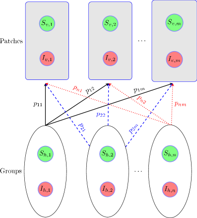
Refer to caption
Figure 1: Flow diagram of the model
Table 1: Description of the parameters used in System (4).
Parameters Description
βvhsubscript𝛽𝑣\beta_{vh} Infectiousness of human to mosquitoes per biting
βhvsubscript𝛽𝑣\beta_{hv} Infectiousness of mosquitoes to humans per biting
ajsubscript𝑎𝑗a_{j} Biting rate in Patch j𝑗j
μisubscript𝜇𝑖\mu_{i} Per capita humans’ birth and death rate for Group i𝑖i
γisubscript𝛾𝑖\gamma_{i} Per capita Recovery rate for Group i𝑖i
pijsubscript𝑝𝑖𝑗p_{ij} Proportion of time individual in Group i𝑖i spend in Patch j𝑗j
μvsubscript𝜇𝑣\mu_{v} Per capita natural death rate of mosquitoes
δjsubscript𝛿𝑗\delta_{j} Per capita death rate of control of mosquitoes in Patch j𝑗j.

The total host population is constant and since total vector population dynamics are given by

N˙v,j=Λv,j(μv+δj)Nv,j,subscript˙𝑁𝑣𝑗subscriptΛ𝑣𝑗subscript𝜇𝑣subscript𝛿𝑗subscript𝑁𝑣𝑗\dot{N}_{v,j}=\Lambda_{v,j}-(\mu_{v}+\delta_{j})N_{v,j},

we can deduce that

lim supt+Nv,j=Λv,jμv+δj:=N¯v,jsubscriptlimit-supremum𝑡subscript𝑁𝑣𝑗subscriptΛ𝑣𝑗subscript𝜇𝑣subscript𝛿𝑗assignsubscript¯𝑁𝑣𝑗\limsup_{t\to+\infty}N_{v,j}=\frac{\Lambda_{v,j}}{\mu_{v}+\delta_{j}}:=\bar{N}_{v,j}

And so, the vector population is asymptotically constant in each patch. The use of the asymptotic theory on triangular systems [12, 72], applied to System (4), leads to the following equivalent autonomous system:

{I˙h,i=βvh(Nh,iIh,i)j=1majpijIv,jk=1npkjNh,k(μi+γi)Ih,i,i=1,2.,n.I˙v,j=ajβhv(N¯v,jIv,j)i=1npijIh,ik=1npkjNh,k(μv+δj)Iv,j,j=1,2,,m.casesformulae-sequenceformulae-sequencesubscript˙𝐼𝑖subscript𝛽𝑣subscript𝑁𝑖subscript𝐼𝑖superscriptsubscript𝑗1𝑚subscript𝑎𝑗subscript𝑝𝑖𝑗subscript𝐼𝑣𝑗superscriptsubscript𝑘1𝑛subscript𝑝𝑘𝑗subscript𝑁𝑘subscript𝜇𝑖subscript𝛾𝑖subscript𝐼𝑖for-all𝑖12𝑛missing-subexpressionmissing-subexpressionmissing-subexpressionmissing-subexpressionmissing-subexpressionmissing-subexpressionmissing-subexpressionformulae-sequencesubscript˙𝐼𝑣𝑗subscript𝑎𝑗subscript𝛽𝑣subscript¯𝑁𝑣𝑗subscript𝐼𝑣𝑗superscriptsubscript𝑖1𝑛subscript𝑝𝑖𝑗subscript𝐼𝑖superscriptsubscript𝑘1𝑛subscript𝑝𝑘𝑗subscript𝑁𝑘subscript𝜇𝑣subscript𝛿𝑗subscript𝐼𝑣𝑗for-all𝑗12𝑚missing-subexpressionmissing-subexpressionmissing-subexpression\left\{\begin{array}[]{llll}\dot{I}_{h,i}=\beta_{vh}(N_{h,i}-I_{h,i})\sum_{j=1}^{m}a_{j}p_{ij}\frac{I_{v,j}}{\sum_{k=1}^{n}p_{kj}N_{h,k}}-(\mu_{i}+\gamma_{i})I_{h,i},\quad\forall i=1,2.\dots,n.\\ \\ \dot{I}_{v,j}=a_{j}\beta_{hv}(\bar{N}_{v,j}-I_{v,j})\frac{\sum_{i=1}^{n}p_{ij}I_{h,i}}{\sum_{k=1}^{n}p_{kj}N_{h,k}}-(\mu_{v}+\delta_{j})I_{v,j},\quad\forall j=1,2,\dots,m.\end{array}\right. (5)

Here, we have that human risk in Patch j𝑗j is defined by ajβvhsubscript𝑎𝑗subscript𝛽𝑣a_{j}\beta_{vh} and so, Patch j𝑗j is riskier than Patch l𝑙l whenever aj>alsubscript𝑎𝑗subscript𝑎𝑙a_{j}>a_{l}. The modeling framework is quite flexible. For example, the case n=m𝑛𝑚n=m covers the interactions between n𝑛n host groups (or classes) in n𝑛n patches or the case when hosts and vectors are co-residents. The case pij=0subscript𝑝𝑖𝑗0p_{ij}=0 for all ji𝑗𝑖j\neq i or pii=1subscript𝑝𝑖𝑖1p_{ii}=1 when n=m𝑛𝑚n=m leads to a collection of isolated classical Ross-Macdonal models. For nm𝑛𝑚n\neq m, hosts are structured in groups like children, farmers, retired people and vectors are distributed in patches or meeting places like home, school, farm, work place or mosquito breeding site, etc. People from the considered groups visit patches and spend certain amount of time and get possibly infected whereby.

Dye and Hasibeder [25, 33] models involve n𝑛n host and m𝑚m vector patches under the assumption that only the vectors move. The models in [18, 58, 64], have incorporated residence times explicitly but their modeling does not account for the effective patch population size. In fact, in[18, 58], the pattern of movement between patches does not produce any “net” change on the total population per patch at any given time. For example, it is assumed (in [58]), that the total population of patch j𝑗j is N/k𝑁𝑘N/k where N𝑁N the overall human population and k𝑘k the number of patches. In [18, 64], the total population in each patch j𝑗j is Njsubscript𝑁𝑗N_{j} (or Hjsubscript𝐻𝑗H_{j} in their notations) regardless of the movement of individuals between patches. Similar remarks hold for the Dengue’s two-patch model in [42]. In our case, the host population in each patch is the sum of visiting individuals of different groups weighted by the proportion of time they spend in each patch. This means that, at time t𝑡t, at any given Patch j𝑗j, the host population is p1jNh,1+p2jNh,2++pnjNh,nsubscript𝑝1𝑗subscript𝑁1subscript𝑝2𝑗subscript𝑁2subscript𝑝𝑛𝑗subscript𝑁𝑛p_{1j}N_{h,1}+p_{2j}N_{h,2}+\dots+p_{nj}N_{h,n}, the effective population size of Patch j𝑗j. Moreover, this approach is well suited for better intervention strategies through the knowledge of ajsubscript𝑎𝑗a_{j}, j=1,,m𝑗1𝑚j=1,\dots,m or the residence time matrix =(pij)1in,1jmsubscriptsubscript𝑝𝑖𝑗1𝑖𝑛1𝑗𝑚\mathbb{P}=(p_{ij})_{\begin{subarray}{c}1\leq i\leq n,\\ 1\leq j\leq m\end{subarray}}. For example, if a particular host group is more affected by the disease in consideration, that may lead to the patch within which the infection had occurred, that is the patch “source” of infection. That could help steer control measures such as DDT in the “infectious” patch or social distancing the “infected” group to mitigate the disease burden.

System (5), could be written in a compact form as follows

{I˙h=βvhdiag(NhIh)diag(a)diag(tNh)1Ivdiag(μ+γ)IhI˙v=βhvdiag(a)diag(NvIv)diag(tNh)1tIhdiag(μv+δ)Ivcasessubscript˙𝐼subscript𝛽𝑣diagsubscript𝑁subscript𝐼diag𝑎diagsuperscriptsuperscript𝑡subscript𝑁1subscript𝐼𝑣diag𝜇𝛾subscript𝐼missing-subexpressionmissing-subexpressionmissing-subexpressionmissing-subexpressionmissing-subexpressionmissing-subexpressionmissing-subexpressionsubscript˙𝐼𝑣subscript𝛽𝑣diag𝑎diagsubscript𝑁𝑣subscript𝐼𝑣diagsuperscriptsuperscript𝑡subscript𝑁1superscript𝑡subscript𝐼diagsubscript𝜇𝑣𝛿subscript𝐼𝑣missing-subexpressionmissing-subexpressionmissing-subexpression\left\{\begin{array}[]{llll}\dot{I}_{h}=\beta_{vh}\textrm{diag}(N_{h}-I_{h})\mathbb{P}\textrm{diag}(a)\textrm{diag}(\mathbb{P}^{t}N_{h})^{-1}I_{v}-\textrm{diag}(\mu+\gamma)I_{h}\\ \\ \dot{I}_{v}=\beta_{hv}\textrm{diag}(a)\textrm{diag}(N_{v}-I_{v})\textrm{diag}(\mathbb{P}^{t}N_{h})^{-1}\mathbb{P}^{t}I_{h}-\textrm{diag}(\mu_{v}+\delta)I_{v}\end{array}\right. (6)

where Ih=[Ih,1,Ih,2,,Ih,n]tsubscript𝐼superscriptsubscript𝐼1subscript𝐼2subscript𝐼𝑛𝑡I_{h}=[I_{h,1},I_{h,2},\dots,I_{h,n}]^{t}, Iv=[Iv,1,Iv,2,,Iv,m]tsubscript𝐼𝑣superscriptsubscript𝐼𝑣1subscript𝐼𝑣2subscript𝐼𝑣𝑚𝑡I_{v}=[I_{v,1},I_{v,2},\dots,I_{v,m}]^{t}, Nh=[Nh,1,Nh,2,,Nh,n]tsubscript𝑁superscriptsubscript𝑁1subscript𝑁2subscript𝑁𝑛𝑡N_{h}=[N_{h,1},N_{h,2},\dots,N_{h,n}]^{t}, N¯v=[N¯v,1,N¯v,2,,N¯v,m]tsubscript¯𝑁𝑣superscriptsubscript¯𝑁𝑣1subscript¯𝑁𝑣2subscript¯𝑁𝑣𝑚𝑡\bar{N}_{v}=[\bar{N}_{v,1},\bar{N}_{v,2},\dots,\bar{N}_{v,m}]^{t}, δ=[δ1,δ2,,δm]t𝛿superscriptsubscript𝛿1subscript𝛿2subscript𝛿𝑚𝑡\delta=[\delta_{1},\delta_{2},\dots,\delta_{m}]^{t}, a=[a1,a2,,am]t𝑎superscriptsubscript𝑎1subscript𝑎2subscript𝑎𝑚𝑡a=[a_{1},a_{2},\dots,a_{m}]^{t} and μ=[μ1,μ2,,μn]t𝜇superscriptsubscript𝜇1subscript𝜇2subscript𝜇𝑛𝑡\mu=[\mu_{1},\mu_{2},\dots,\mu_{n}]^{t}.

We end this section by showing that the solutions of Model (5) are positive and bounded, or in other words, that the model is biologically grounded.

Lemma 1.1.

The region defined by

Ω={(Ih,Iv)+n+m  IhNh,IvN¯v}\Omega=\left\{(I_{h},I_{v})\in\mathbb{R}^{n+m}_{+}\;\mbox{ \LARGE$\mid$ }\;I_{h}\leq N_{h},\;\;I_{v}\leq\bar{N}_{v}\right\}

is a compact attracting positively invariant set for System (6) .

Proof.

The set ΩΩ\Omega, a subset n+msuperscript𝑛𝑚\mathbb{R}^{n+m}, is clearly closed and bounded and hence a compact. The right-hand side of System (6) could be written as A(Ih,Iv)(Ih,Iv)t𝐴subscript𝐼subscript𝐼𝑣superscriptsubscript𝐼subscript𝐼𝑣𝑡A(I_{h},I_{v})(I_{h},I_{v})^{t} where

A(Ih,Iv)=(diag(μ+γ)βvhdiag(NhIh)diag(a)diag(tNh)1βhvdiag(a)diag(N¯vIv)diag(tNh)1tdiag(μv+δ))𝐴subscript𝐼subscript𝐼𝑣diag𝜇𝛾subscript𝛽𝑣diagsubscript𝑁subscript𝐼diag𝑎diagsuperscriptsuperscript𝑡subscript𝑁1subscript𝛽𝑣diag𝑎diagsubscript¯𝑁𝑣subscript𝐼𝑣diagsuperscriptsuperscript𝑡subscript𝑁1superscript𝑡diagsubscript𝜇𝑣𝛿A(I_{h},I_{v})=\left(\begin{array}[]{cc}-\textrm{diag}(\mu+\gamma)&\beta_{vh}\textrm{diag}(N_{h}-I_{h})\mathbb{P}\textrm{diag}(a)\textrm{diag}(\mathbb{P}^{t}N_{h})^{-1}\\ \beta_{hv}\textrm{diag}(a)\textrm{diag}(\bar{N}_{v}-I_{v})\textrm{diag}(\mathbb{P}^{t}N_{h})^{-1}\mathbb{P}^{t}&-\textrm{diag}(\mu_{v}+\delta)\end{array}\right)

Since, InNhsubscript𝐼𝑛subscript𝑁I_{n}\leq N_{h} and IvN¯vsubscript𝐼𝑣subscript¯𝑁𝑣I_{v}\leq\bar{N}_{v}, the matrix A(Ih,Iv)𝐴subscript𝐼subscript𝐼𝑣A(I_{h},I_{v}) is Metzler. Hence, the positive orthant +n+msubscriptsuperscript𝑛𝑚\mathbb{R}^{n+m}_{+} is invariant. At Ih=Nhsubscript𝐼subscript𝑁I_{h}=N_{h}, we have I˙h=diag(μ+γ)Ih0subscript˙𝐼diag𝜇𝛾subscript𝐼0\dot{I}_{h}=-\textrm{diag}(\mu+\gamma)I_{h}\leq 0. Similarly, at Iv=N¯vsubscript𝐼𝑣subscript¯𝑁𝑣I_{v}=\bar{N}_{v}, we have I˙v=diag(μv+δ)Iv0subscript˙𝐼𝑣diagsubscript𝜇𝑣𝛿subscript𝐼𝑣0\dot{I}_{v}=-\textrm{diag}(\mu_{v}+\delta)I_{v}\leq 0. Hence, the vector field of (6) is pointed inward from the faces of ΩΩ\Omega. ∎

2 Equilibria and Global Stability

In the absence of infected vectors in all patches, Model (6) supports a unique, disease free equilibrium (DFE), given by E0=0n+msubscript𝐸0subscript0superscript𝑛𝑚E_{0}=\textbf{0}_{\mathbb{R}^{n+m}}. The basic reproduction number, defined as the average number of secondary cases produced of by an infected individual during its lifetime, is computed using the next generation method [19, 71]. The right hand side of (6) could be written as +𝒱𝒱\mathcal{F}+\mathcal{V} where

(Ih,Iv)=(βvhdiag(Nh)diag(a)diag(tNh)1Ivβhvdiag(a)diag(Nv)diag(tNh)1tIh)and𝒱(Ih,Iv)=(diag(μ+γ)Ihdiag(μv+δ)Iv)formulae-sequencesubscript𝐼subscript𝐼𝑣subscript𝛽𝑣diagsubscript𝑁diag𝑎diagsuperscriptsuperscript𝑡subscript𝑁1subscript𝐼𝑣subscript𝛽𝑣diag𝑎diagsubscript𝑁𝑣diagsuperscriptsuperscript𝑡subscript𝑁1superscript𝑡subscript𝐼and𝒱subscript𝐼subscript𝐼𝑣diag𝜇𝛾subscript𝐼diagsubscript𝜇𝑣𝛿subscript𝐼𝑣\mathcal{F}(I_{h},I_{v})=\left(\begin{array}[]{c}\beta_{vh}\textrm{diag}(N_{h})\mathbb{P}\textrm{diag}(a)\textrm{diag}(\mathbb{P}^{t}N_{h})^{-1}I_{v}\\ \beta_{hv}\textrm{diag}(a)\textrm{diag}(N_{v})\textrm{diag}(\mathbb{P}^{t}N_{h})^{-1}\mathbb{P}^{t}I_{h}\end{array}\right)\quad\textrm{and}\quad\mathcal{V}(I_{h},I_{v})=\left(\begin{array}[]{c}-\textrm{diag}(\mu+\gamma)I_{h}\\ -\textrm{diag}(\mu_{v}+\delta)I_{v}\end{array}\right)

Let F=D(Ih,Iv)𝐹𝐷subscript𝐼subscript𝐼𝑣F=D\mathcal{F}(I_{h},I_{v}) and V=D𝒱(Ih,Iv)𝑉𝐷𝒱subscript𝐼subscript𝐼𝑣V=D\mathcal{V}(I_{h},I_{v}) evaluated at the DFE. We obtain:

F=(0βvhdiag(Nh)diag(a)diag(tNh)1βhvdiag(a)diag(Nv)diag(tNh)1t0)𝐹0subscript𝛽𝑣diagsubscript𝑁diag𝑎diagsuperscriptsuperscript𝑡subscript𝑁1subscript𝛽𝑣diag𝑎diagsubscript𝑁𝑣diagsuperscriptsuperscript𝑡subscript𝑁1superscript𝑡0F=\left(\begin{array}[]{cc}0&\beta_{vh}\textrm{diag}(N_{h})\mathbb{P}\textrm{diag}(a)\textrm{diag}(\mathbb{P}^{t}N_{h})^{-1}\\ \beta_{hv}\textrm{diag}(a)\textrm{diag}(N_{v})\textrm{diag}(\mathbb{P}^{t}N_{h})^{-1}\mathbb{P}^{t}&0\end{array}\right)

and

V=(Vh00Vv)𝑉subscript𝑉00subscript𝑉𝑣V=\left(\begin{array}[]{cc}-V_{h}&0\\ 0&-V_{v}\end{array}\right)

where Vh=diag(μ+γ)subscript𝑉diag𝜇𝛾V_{h}=\textrm{diag}(\mu+\gamma) and Vv=diag(μv+δ)subscript𝑉𝑣diagsubscript𝜇𝑣𝛿V_{v}=\textrm{diag}(\mu_{v}+\delta).
The basic reproduction number is the spectral radius of the next generation matrix:

FV1=(0n,nMvhMhv0m,m)𝐹superscript𝑉1subscript0𝑛𝑛subscript𝑀𝑣missing-subexpressionmissing-subexpressionsubscript𝑀𝑣subscript0𝑚𝑚missing-subexpressionmissing-subexpression-FV^{-1}=\left(\begin{array}[]{cccc}\textbf{0}_{n,n}&M_{vh}\\ M_{hv}&\textbf{0}_{m,m}\end{array}\right)

where

Mhv=βhvdiag(a)diag(tNh)1diag(Nv)tVh1subscript𝑀𝑣subscript𝛽𝑣diag𝑎diagsuperscriptsuperscript𝑡subscript𝑁1diagsubscript𝑁𝑣superscript𝑡superscriptsubscript𝑉1M_{hv}=\beta_{hv}\textrm{diag}(a)\textrm{diag}(\mathbb{P}^{t}N_{h})^{-1}\textrm{diag}(N_{v})\mathbb{P}^{t}V_{h}^{-1}

and

Mvh=βvhdiag(Nh)diag(tNh)1diag(a)Vv1subscript𝑀𝑣subscript𝛽𝑣diagsubscript𝑁diagsuperscriptsuperscript𝑡subscript𝑁1diag𝑎superscriptsubscript𝑉𝑣1M_{vh}=\beta_{vh}\textrm{diag}(N_{h})\mathbb{P}\textrm{diag}(\mathbb{P}^{t}N_{h})^{-1}\textrm{diag}(a)V_{v}^{-1}

Notice also that since (FV)2=diag(Mvh,Mhv)superscript𝐹𝑉2diagsubscript𝑀𝑣subscript𝑀𝑣(-FV)^{2}=\textrm{diag}(M_{vh},M_{hv}), we can deduce that the basic reproduction number is 02=ρ(MvhMhv)superscriptsubscript02𝜌subscript𝑀𝑣subscript𝑀𝑣\mathcal{R}_{0}^{2}=\rho(M_{vh}M_{hv}).

More precisely, we have that

Mhv=(a1βhvp11Nv,1i=1npi1Nh,i(μ1+γ1)a1βhvp21Nv,1i=1npi1Nh,i(μ2+γ2)a1βhvpn1Nv,1i=1npi1Nh,i(μn+γn)a2βhvp12Nv,2i=1npi2Nh,i(μ1+γ1)a2βhvp22Nv,2i=1npi2Nh,i(μ2+γ2)a2βhvpn2Nv,2i=1npi2Nh,i(μn+γn)amβhvp1mNv,mi=1npimNh,i(μ1+γ1)amβhvp2mNv,mi=1npimNh,i(μ2+γ2)amβhvpnmNv,mi=1npimNh,i(μn+γn))subscript𝑀𝑣subscript𝑎1subscript𝛽𝑣subscript𝑝11subscript𝑁𝑣1superscriptsubscript𝑖1𝑛subscript𝑝𝑖1subscript𝑁𝑖subscript𝜇1subscript𝛾1subscript𝑎1subscript𝛽𝑣subscript𝑝21subscript𝑁𝑣1superscriptsubscript𝑖1𝑛subscript𝑝𝑖1subscript𝑁𝑖subscript𝜇2subscript𝛾2subscript𝑎1subscript𝛽𝑣subscript𝑝𝑛1subscript𝑁𝑣1superscriptsubscript𝑖1𝑛subscript𝑝𝑖1subscript𝑁𝑖subscript𝜇𝑛subscript𝛾𝑛subscript𝑎2subscript𝛽𝑣subscript𝑝12subscript𝑁𝑣2superscriptsubscript𝑖1𝑛subscript𝑝𝑖2subscript𝑁𝑖subscript𝜇1subscript𝛾1subscript𝑎2subscript𝛽𝑣subscript𝑝22subscript𝑁𝑣2superscriptsubscript𝑖1𝑛subscript𝑝𝑖2subscript𝑁𝑖subscript𝜇2subscript𝛾2subscript𝑎2subscript𝛽𝑣subscript𝑝𝑛2subscript𝑁𝑣2superscriptsubscript𝑖1𝑛subscript𝑝𝑖2subscript𝑁𝑖subscript𝜇𝑛subscript𝛾𝑛subscript𝑎𝑚subscript𝛽𝑣subscript𝑝1𝑚subscript𝑁𝑣𝑚superscriptsubscript𝑖1𝑛subscript𝑝𝑖𝑚subscript𝑁𝑖subscript𝜇1subscript𝛾1subscript𝑎𝑚subscript𝛽𝑣subscript𝑝2𝑚subscript𝑁𝑣𝑚superscriptsubscript𝑖1𝑛subscript𝑝𝑖𝑚subscript𝑁𝑖subscript𝜇2subscript𝛾2subscript𝑎𝑚subscript𝛽𝑣subscript𝑝𝑛𝑚subscript𝑁𝑣𝑚superscriptsubscript𝑖1𝑛subscript𝑝𝑖𝑚subscript𝑁𝑖subscript𝜇𝑛subscript𝛾𝑛M_{hv}=\left(\begin{array}[]{cccc}\frac{a_{1}\beta_{hv}p_{11}N_{v,1}}{\sum_{i=1}^{n}p_{i1}N_{h,i}(\mu_{1}+\gamma_{1})}&\frac{a_{1}\beta_{hv}p_{21}N_{v,1}}{\sum_{i=1}^{n}p_{i1}N_{h,i}(\mu_{2}+\gamma_{2})}&\cdots&\frac{a_{1}\beta_{hv}p_{n1}N_{v,1}}{\sum_{i=1}^{n}p_{i1}N_{h,i}(\mu_{n}+\gamma_{n})}\\ \frac{a_{2}\beta_{hv}p_{12}N_{v,2}}{\sum_{i=1}^{n}p_{i2}N_{h,i}(\mu_{1}+\gamma_{1})}&\frac{a_{2}\beta_{hv}p_{22}N_{v,2}}{\sum_{i=1}^{n}p_{i2}N_{h,i}(\mu_{2}+\gamma_{2})}&\cdots&\frac{a_{2}\beta_{hv}p_{n2}N_{v,2}}{\sum_{i=1}^{n}p_{i2}N_{h,i}(\mu_{n}+\gamma_{n})}\\ \vdots&\vdots&\cdots&\vdots\\ \frac{a_{m}\beta_{hv}p_{1m}N_{v,m}}{\sum_{i=1}^{n}p_{im}N_{h,i}(\mu_{1}+\gamma_{1})}&\frac{a_{m}\beta_{hv}p_{2m}N_{v,m}}{\sum_{i=1}^{n}p_{im}N_{h,i}(\mu_{2}+\gamma_{2})}&\cdots&\frac{a_{m}\beta_{hv}p_{nm}N_{v,m}}{\sum_{i=1}^{n}p_{im}N_{h,i}(\mu_{n}+\gamma_{n})}\end{array}\right)

and

Mvh=(a1βvhp11Nh,1i=1npi1Nh,i(μv+δ1)a2βvhp12Nh,1i=1npi2Nh,i(μv+δ2)amβhvp1mNh,1i=1npimNh,i(μv+δm)a1βvhp21Nh,2i=1npi1Nh,i(μv+δ1)a2βvhp22Nh,2i=1npi2Nh,i(μv+δ2)amβvhp2mNh,2i=1npimNh,i(μv+δm)a1βvhpn1Nh,ni=1npi1Nh,i(μv+δ1)a2βvhpn2Nh,ni=1npi2Nh,i(μv+δ2)amβhvpnmNh,ni=1npimNh,i(μv+δm))subscript𝑀𝑣subscript𝑎1subscript𝛽𝑣subscript𝑝11subscript𝑁1superscriptsubscript𝑖1𝑛subscript𝑝𝑖1subscript𝑁𝑖subscript𝜇𝑣subscript𝛿1subscript𝑎2subscript𝛽𝑣subscript𝑝12subscript𝑁1superscriptsubscript𝑖1𝑛subscript𝑝𝑖2subscript𝑁𝑖subscript𝜇𝑣subscript𝛿2subscript𝑎𝑚subscript𝛽𝑣subscript𝑝1𝑚subscript𝑁1superscriptsubscript𝑖1𝑛subscript𝑝𝑖𝑚subscript𝑁𝑖subscript𝜇𝑣subscript𝛿𝑚subscript𝑎1subscript𝛽𝑣subscript𝑝21subscript𝑁2superscriptsubscript𝑖1𝑛subscript𝑝𝑖1subscript𝑁𝑖subscript𝜇𝑣subscript𝛿1subscript𝑎2subscript𝛽𝑣subscript𝑝22subscript𝑁2superscriptsubscript𝑖1𝑛subscript𝑝𝑖2subscript𝑁𝑖subscript𝜇𝑣subscript𝛿2subscript𝑎𝑚subscript𝛽𝑣subscript𝑝2𝑚subscript𝑁2superscriptsubscript𝑖1𝑛subscript𝑝𝑖𝑚subscript𝑁𝑖subscript𝜇𝑣subscript𝛿𝑚subscript𝑎1subscript𝛽𝑣subscript𝑝𝑛1subscript𝑁𝑛superscriptsubscript𝑖1𝑛subscript𝑝𝑖1subscript𝑁𝑖subscript𝜇𝑣subscript𝛿1subscript𝑎2subscript𝛽𝑣subscript𝑝𝑛2subscript𝑁𝑛superscriptsubscript𝑖1𝑛subscript𝑝𝑖2subscript𝑁𝑖subscript𝜇𝑣subscript𝛿2subscript𝑎𝑚subscript𝛽𝑣subscript𝑝𝑛𝑚subscript𝑁𝑛superscriptsubscript𝑖1𝑛subscript𝑝𝑖𝑚subscript𝑁𝑖subscript𝜇𝑣subscript𝛿𝑚M_{vh}=\left(\begin{array}[]{cccc}\frac{a_{1}\beta_{vh}p_{11}N_{h,1}}{\sum_{i=1}^{n}p_{i1}N_{h,i}(\mu_{v}+\delta_{1})}&\frac{a_{2}\beta_{vh}p_{12}N_{h,1}}{\sum_{i=1}^{n}p_{i2}N_{h,i}(\mu_{v}+\delta_{2})}&\cdots&\frac{a_{m}\beta_{hv}p_{1m}N_{h,1}}{\sum_{i=1}^{n}p_{im}N_{h,i}(\mu_{v}+\delta_{m})}\\ \frac{a_{1}\beta_{vh}p_{21}N_{h,2}}{\sum_{i=1}^{n}p_{i1}N_{h,i}(\mu_{v}+\delta_{1})}&\frac{a_{2}\beta_{vh}p_{22}N_{h,2}}{\sum_{i=1}^{n}p_{i2}N_{h,i}(\mu_{v}+\delta_{2})}&\cdots&\frac{a_{m}\beta_{vh}p_{2m}N_{h,2}}{\sum_{i=1}^{n}p_{im}N_{h,i}(\mu_{v}+\delta_{m})}\\ \vdots&\vdots&\cdots&\vdots\\ \frac{a_{1}\beta_{vh}p_{n1}N_{h,n}}{\sum_{i=1}^{n}p_{i1}N_{h,i}(\mu_{v}+\delta_{1})}&\frac{a_{2}\beta_{vh}p_{n2}N_{h,n}}{\sum_{i=1}^{n}p_{i2}N_{h,i}(\mu_{v}+\delta_{2})}&\cdots&\frac{a_{m}\beta_{hv}p_{nm}N_{h,n}}{\sum_{i=1}^{n}p_{im}N_{h,i}(\mu_{v}+\delta_{m})}\end{array}\right)

Note that the matrices Mhvsubscript𝑀𝑣M_{hv} and Mvhsubscript𝑀𝑣M_{vh} are of (m,n)𝑚𝑛(m,n) and (n,m)𝑛𝑚(n,m) size respectively. The matrix Mvhsubscript𝑀𝑣M_{vh} represents the new human cases due to infected mosquitoes whereas Mhvsubscript𝑀𝑣M_{hv} represents the new mosquito cases due to humans. In fact, the elements of Mvhsubscript𝑀𝑣M_{vh} and Mhvsubscript𝑀𝑣M_{hv} have specific biological interpretations, for instance,

  • For i=1,,n𝑖1𝑛i=1,\dots,n and j=1,,m𝑗1𝑚j=1,\dots,m, we have (mhv)ji=ajβhvpijN¯v,j(μi+γi)l=1npljNh,lsubscriptsubscript𝑚𝑣𝑗𝑖subscript𝑎𝑗subscript𝛽𝑣subscript𝑝𝑖𝑗subscript¯𝑁𝑣𝑗subscript𝜇𝑖subscript𝛾𝑖superscriptsubscript𝑙1𝑛subscript𝑝𝑙𝑗subscript𝑁𝑙(m_{hv})_{ji}=\frac{a_{j}\beta_{hv}p_{ij}\bar{N}_{v,j}}{(\mu_{i}+\gamma_{i})\sum_{l=1}^{n}p_{lj}N_{h,l}} represents the average number of secondary vector (of Patch j𝑗j) cases of infection produced by a single infected of group i𝑖i during his/her infectious period.

  • Similarly, for i=1,,n𝑖1𝑛i=1,\dots,n and j=1,,m𝑗1𝑚j=1,\dots,m, we have (mvh)ij=ajβhvpijNh,i(μv+δj)l=1npljNh,lsubscriptsubscript𝑚𝑣𝑖𝑗subscript𝑎𝑗subscript𝛽𝑣subscript𝑝𝑖𝑗subscript𝑁𝑖subscript𝜇𝑣subscript𝛿𝑗superscriptsubscript𝑙1𝑛subscript𝑝𝑙𝑗subscript𝑁𝑙(m_{vh})_{ij}=\frac{a_{j}\beta_{hv}p_{ij}N_{h,i}}{(\mu_{v}+\delta_{j})\sum_{l=1}^{n}p_{lj}N_{h,l}} represents the average number of secondary human (of group i𝑖i) cases generated by an infected vector (of Patch j𝑗j) during her infectious period.

  • The overall number of new cases produced by an infected mosquitoes in Patch j𝑗j is the sum of the elements of the jthsuperscript𝑗𝑡j^{th} column of Mvhsubscript𝑀𝑣M_{vh}, that is,

    i=1n(mvh)ijsuperscriptsubscript𝑖1𝑛subscriptsubscript𝑚𝑣𝑖𝑗\displaystyle\sum_{i=1}^{n}(m_{vh})_{ij} =\displaystyle= i=1najβhvpijNh,i(μv+δj)l=1npljNh,lsuperscriptsubscript𝑖1𝑛subscript𝑎𝑗subscript𝛽𝑣subscript𝑝𝑖𝑗subscript𝑁𝑖subscript𝜇𝑣subscript𝛿𝑗superscriptsubscript𝑙1𝑛subscript𝑝𝑙𝑗subscript𝑁𝑙\displaystyle\sum_{i=1}^{n}\frac{a_{j}\beta_{hv}p_{ij}N_{h,i}}{(\mu_{v}+\delta_{j})\sum_{l=1}^{n}p_{lj}N_{h,l}}
    =\displaystyle= ajβhv(μv+δj)l=1npljNh,li=1npijNh,isubscript𝑎𝑗subscript𝛽𝑣subscript𝜇𝑣subscript𝛿𝑗superscriptsubscript𝑙1𝑛subscript𝑝𝑙𝑗subscript𝑁𝑙superscriptsubscript𝑖1𝑛subscript𝑝𝑖𝑗subscript𝑁𝑖\displaystyle\frac{a_{j}\beta_{hv}}{(\mu_{v}+\delta_{j})\sum_{l=1}^{n}p_{lj}N_{h,l}}\sum_{i=1}^{n}p_{ij}N_{h,i}
    =\displaystyle= ajβhv(μv+δj).subscript𝑎𝑗subscript𝛽𝑣subscript𝜇𝑣subscript𝛿𝑗\displaystyle\frac{a_{j}\beta_{hv}}{(\mu_{v}+\delta_{j})}.

The overall new vector cases generated by an infected human of group i𝑖i is the sum of the first column of Mhvsubscript𝑀𝑣M_{hv}, namely,

j=1m(mhv)jisuperscriptsubscript𝑗1𝑚subscriptsubscript𝑚𝑣𝑗𝑖\displaystyle\sum_{j=1}^{m}(m_{hv})_{ji} =\displaystyle= j=1majβhvpijN¯v,j(μi+γi)l=1npljNh,lsuperscriptsubscript𝑗1𝑚subscript𝑎𝑗subscript𝛽𝑣subscript𝑝𝑖𝑗subscript¯𝑁𝑣𝑗subscript𝜇𝑖subscript𝛾𝑖superscriptsubscript𝑙1𝑛subscript𝑝𝑙𝑗subscript𝑁𝑙\displaystyle\sum_{j=1}^{m}\frac{a_{j}\beta_{hv}p_{ij}\bar{N}_{v,j}}{(\mu_{i}+\gamma_{i})\sum_{l=1}^{n}p_{lj}N_{h,l}}
=\displaystyle= βhv(μi+γi)j=1majpijN¯v,jl=1npljNh,l.subscript𝛽𝑣subscript𝜇𝑖subscript𝛾𝑖superscriptsubscript𝑗1𝑚subscript𝑎𝑗subscript𝑝𝑖𝑗subscript¯𝑁𝑣𝑗superscriptsubscript𝑙1𝑛subscript𝑝𝑙𝑗subscript𝑁𝑙\displaystyle\frac{\beta_{hv}}{(\mu_{i}+\gamma_{i})}\sum_{j=1}^{m}\frac{a_{j}p_{ij}\bar{N}_{v,j}}{\sum_{l=1}^{n}p_{lj}N_{h,l}}.

The matrix

(0MvhMvh0)0subscript𝑀𝑣subscript𝑀𝑣0\left(\begin{array}[]{cc}0&M_{vh}\\ M_{vh}&0\end{array}\right)

or equivalently the matrix

(0𝒩vh𝒩vh0)0subscript𝒩𝑣subscript𝒩𝑣0\left(\begin{array}[]{cc}0&\mathcal{N}_{vh}\\ \mathcal{N}_{vh}&0\end{array}\right)

where 𝒩vh=diag(Nh)diag(tNh)1diag(a)subscript𝒩𝑣diagsubscript𝑁diagsuperscriptsuperscript𝑡subscript𝑁1diag𝑎\mathcal{N}_{vh}=\textrm{diag}(N_{h})\mathbb{P}\textrm{diag}(\mathbb{P}^{t}N_{h})^{-1}\textrm{diag}(a) and 𝒩hv=diag(a)diag(tNh)1diag(N¯v)tsubscript𝒩𝑣diag𝑎diagsuperscriptsuperscript𝑡subscript𝑁1diagsubscript¯𝑁𝑣superscript𝑡\mathcal{N}_{hv}=\textrm{diag}(a)\textrm{diag}(\mathbb{P}^{t}N_{h})^{-1}\textrm{diag}(\bar{N}_{v})\mathbb{P}^{t} is what authors in [36] called host-vector network. It is proven in [36] that the matrix FV1𝐹superscript𝑉1-FV^{-1} is irreducible if and only if MhvMvhsubscript𝑀𝑣subscript𝑀𝑣M_{hv}M_{vh} and MvhMhvsubscript𝑀𝑣subscript𝑀𝑣M_{vh}M_{hv} are both irreducible. Notice that, even if n=m𝑛𝑚n=m, the irreducibility of \mathbb{P} is neither necessary nor sufficient to ensure the irreducibility of MhvMvhsubscript𝑀𝑣subscript𝑀𝑣M_{hv}M_{vh} and MvhMhvsubscript𝑀𝑣subscript𝑀𝑣M_{vh}M_{hv}. See the subsection 4.1 for counter examples.

Remark 2.1.

If we suppose that n=m𝑛𝑚n=m and pij=0,{i,j}{1,2,,n}2formulae-sequencesubscript𝑝𝑖𝑗0for-all𝑖𝑗superscript12𝑛2p_{ij}=0,\;\;\forall\{i,j\}\in\{1,2,\dots,n\}^{2} and ij𝑖𝑗i\neq j then =Insubscript𝐼𝑛\mathbb{P}=I_{n}. Hence, Mhvsubscript𝑀𝑣M_{hv} and Mvhsubscript𝑀𝑣M_{vh} are diagonal matrices and so is their product MhvMvhsubscript𝑀𝑣subscript𝑀𝑣M_{hv}M_{vh}. Hence,

02=max{(01)2,(02)2,,(0n)2}superscriptsubscript02superscriptsuperscriptsubscript012superscriptsuperscriptsubscript022superscriptsuperscriptsubscript0𝑛2\mathcal{R}_{0}^{2}=\max\{(\mathcal{R}_{0}^{1})^{2},(\mathcal{R}_{0}^{2})^{2},\dots,(\mathcal{R}_{0}^{n})^{2}\}

where

(0i)2=ai2βvhβhvN¯v,iμv(μi+γi)Nh,isuperscriptsuperscriptsubscript0𝑖2superscriptsubscript𝑎𝑖2subscript𝛽𝑣subscript𝛽𝑣subscript¯𝑁𝑣𝑖subscript𝜇𝑣subscript𝜇𝑖subscript𝛾𝑖subscript𝑁𝑖(\mathcal{R}_{0}^{i})^{2}=\frac{a_{i}^{2}\beta_{vh}\beta_{hv}\bar{N}_{v,i}}{\mu_{v}(\mu_{i}+\gamma_{i})N_{h,i}}

For each i𝑖i, the basic reproduction number (0i)2superscriptsuperscriptsubscript0𝑖2(\mathcal{R}_{0}^{i})^{2} is the one derived from the classical Ross model.

Theorem 2.1.

Under the assumption that the host-vector network is irreducible, we have that

  1. 1.

    If 01subscript01\mathcal{R}_{0}\leq 1, the DFE is globally asymptotically stable.

  2. 2.

    If 0>1subscript01\mathcal{R}_{0}>1, the DFE is unstable.

Theorem 2.2.

Under the assumption that the vector-host network is irreducible, we have that if 0>1subscript01\mathcal{R}_{0}>1 then there exists a unique endemic equilibrium that is globally asymptotically stable.

Theorems 2.1 and 2.2 can be obtained by using H. L. Smith’s results [66]. Indeed, it is immediate that System (6) is cooperative, strongly concave and its Jacobian is irreducible. Hence, the theorems can be obtained following Smith’s results [66] (Theorem 3.1 and Corollary 3.2). A similar method using Hirsch’s theorem [34] is outlined by Iggidr et al. in [37] for an SIS𝑆𝐼𝑆SIS metapopulation model.

A sharp threshold results of a multi-group vector-borne disease model has been obtained in [36] by using nicely crafted Lyapunov functions and elements of graph theory.

3 Effects of heterogeneity

In this section, we take a closer look to the effect of heterogeneity on the basic reproduction number and provide simple bounds for the basic reproduction number that may be useful in applications. We also compare the effects of patchiness (the role of variable number of patches/environments) and groupness (the role of variable hosts’ groups) on the basic reproduction number. We denote 02(m,n)superscriptsubscript02𝑚𝑛\mathcal{R}_{0}^{2}(m,n) the basic reproduction number for n𝑛n groups and m𝑚m patches.

The basic reproduction number is the spectral radius of MvhMhvsubscript𝑀𝑣subscript𝑀𝑣M_{vh}M_{hv}. This matrix is supposed irreducible with entries are given by:

rij=βvhβhvNh,iμj+γjk=1mak2pikpjkNv,k(l=1nplkNh,l)2(μv+δk)i,j=1,,n.formulae-sequencesubscript𝑟𝑖𝑗subscript𝛽𝑣subscript𝛽𝑣subscript𝑁𝑖subscript𝜇𝑗subscript𝛾𝑗superscriptsubscript𝑘1𝑚superscriptsubscript𝑎𝑘2subscript𝑝𝑖𝑘subscript𝑝𝑗𝑘subscript𝑁𝑣𝑘superscriptsuperscriptsubscript𝑙1𝑛subscript𝑝𝑙𝑘subscript𝑁𝑙2subscript𝜇𝑣subscript𝛿𝑘for-all𝑖𝑗1𝑛r_{ij}=\frac{\beta_{vh}\beta_{hv}N_{h,i}}{\mu_{j}+\gamma_{j}}\sum_{k=1}^{m}\frac{a_{k}^{2}p_{ik}p_{jk}N_{v,k}}{(\sum_{l=1}^{n}p_{lk}N_{h,l})^{2}(\mu_{v}+\delta_{k})}\quad\forall i,j=1,\dots,n. (7)

=(rij)subscript𝑟𝑖𝑗\mathbb{R}=(r_{ij}) is an n×n𝑛𝑛n\times n matrix. The basic reproduction number is also the spectral radius of MhvMvhsubscript𝑀𝑣subscript𝑀𝑣M_{hv}M_{vh}, a matrix with entries

r~ij=aiajβhvβvhNv,i(μv+δj)(l=1npliNh,l)(l=1npljNh,l)k=1npkipkjNh,kμk+γki,j=1,,m.formulae-sequencesubscript~𝑟𝑖𝑗subscript𝑎𝑖subscript𝑎𝑗subscript𝛽𝑣subscript𝛽𝑣subscript𝑁𝑣𝑖subscript𝜇𝑣subscript𝛿𝑗superscriptsubscript𝑙1𝑛subscript𝑝𝑙𝑖subscript𝑁𝑙superscriptsubscript𝑙1𝑛subscript𝑝𝑙𝑗subscript𝑁𝑙superscriptsubscript𝑘1𝑛subscript𝑝𝑘𝑖subscript𝑝𝑘𝑗subscript𝑁𝑘subscript𝜇𝑘subscript𝛾𝑘for-all𝑖𝑗1𝑚\tilde{r}_{ij}=\frac{a_{i}a_{j}\beta_{hv}\beta_{vh}N_{v,i}}{(\mu_{v}+\delta_{j})(\sum_{l=1}^{n}p_{li}N_{h,l})(\sum_{l=1}^{n}p_{lj}N_{h,l})}\sum_{k=1}^{n}\frac{p_{ki}p_{kj}N_{h,k}}{\mu_{k}+\gamma_{k}}\quad\forall i,j=1,\dots,m. (8)

The next theorem collects a set of inequalities that identify lower and upper bounds for the basic reproduction number.

Theorem 3.1.
  1. 1.

    minj=1,,nLj02(n,m)maxj=1,,nLjsubscript𝑗1𝑛subscript𝐿𝑗superscriptsubscript02𝑛𝑚subscript𝑗1𝑛subscript𝐿𝑗\displaystyle\min_{j=1,\dots,n}L_{j}\leq\mathcal{R}_{0}^{2}(n,m)\leq\max_{j=1,\dots,n}L_{j} where

    Lj=βhvβhvμj+γjk=1mak2pjkNv,k(l=1nplkNh,l)(μv+δk)subscript𝐿𝑗subscript𝛽𝑣subscript𝛽𝑣subscript𝜇𝑗subscript𝛾𝑗superscriptsubscript𝑘1𝑚superscriptsubscript𝑎𝑘2subscript𝑝𝑗𝑘subscript𝑁𝑣𝑘superscriptsubscript𝑙1𝑛subscript𝑝𝑙𝑘subscript𝑁𝑙subscript𝜇𝑣subscript𝛿𝑘L_{j}=\frac{\beta_{hv}\beta_{hv}}{\mu_{j}+\gamma_{j}}\sum_{k=1}^{m}\frac{a_{k}^{2}p_{jk}N_{v,k}}{(\sum_{l=1}^{n}p_{lk}N_{h,l})(\mu_{v}+\delta_{k})}
  2. 2.

    mini=1,,nLi02(n,m)maxi=1,,nLisubscript𝑖1𝑛superscriptsubscript𝐿𝑖superscriptsubscript02𝑛𝑚subscript𝑖1𝑛superscriptsubscript𝐿𝑖\displaystyle\min_{i=1,\dots,n}L_{i}^{\sharp}\leq\mathcal{R}_{0}^{2}(n,m)\leq\max_{i=1,\dots,n}L_{i}^{\sharp} where

    Li=k=1mak2βhvβhvpikNh,iNv,k(l=1nplkNh,l)2(μv+δk)(j=1npjkμj+γj)superscriptsubscript𝐿𝑖superscriptsubscript𝑘1𝑚superscriptsubscript𝑎𝑘2subscript𝛽𝑣subscript𝛽𝑣subscript𝑝𝑖𝑘subscript𝑁𝑖subscript𝑁𝑣𝑘superscriptsuperscriptsubscript𝑙1𝑛subscript𝑝𝑙𝑘subscript𝑁𝑙2subscript𝜇𝑣subscript𝛿𝑘superscriptsubscript𝑗1𝑛subscript𝑝𝑗𝑘subscript𝜇𝑗subscript𝛾𝑗L_{i}^{\sharp}=\sum_{k=1}^{m}\frac{a_{k}^{2}\beta_{hv}\beta_{hv}p_{ik}N_{h,i}N_{v,k}}{(\sum_{l=1}^{n}p_{lk}N_{h,l})^{2}(\mu_{v}+\delta_{k})}\left(\sum_{j=1}^{n}\frac{p_{jk}}{\mu_{j}+\gamma_{j}}\right)
  3. 3.

    minj=1,,mLj02(n,m)maxj=1,,mLjsubscript𝑗1𝑚superscriptsubscript𝐿𝑗superscriptsubscript02𝑛𝑚subscript𝑗1𝑚superscriptsubscript𝐿𝑗\displaystyle\min_{j=1,\dots,m}L_{j}^{\diamond}\leq\mathcal{R}_{0}^{2}(n,m)\leq\max_{j=1,\dots,m}L_{j}^{\diamond} where

    Lj=ajβhvβvh(μv+δj)(l=1npljNh,l)k=1npkjNh,kμk+γk(i=1maipkiNv,il=1npliNh,l)superscriptsubscript𝐿𝑗subscript𝑎𝑗subscript𝛽𝑣subscript𝛽𝑣subscript𝜇𝑣subscript𝛿𝑗superscriptsubscript𝑙1𝑛subscript𝑝𝑙𝑗subscript𝑁𝑙superscriptsubscript𝑘1𝑛subscript𝑝𝑘𝑗subscript𝑁𝑘subscript𝜇𝑘subscript𝛾𝑘superscriptsubscript𝑖1𝑚subscript𝑎𝑖subscript𝑝𝑘𝑖subscript𝑁𝑣𝑖superscriptsubscript𝑙1𝑛subscript𝑝𝑙𝑖subscript𝑁𝑙L_{j}^{\diamond}=\frac{a_{j}\beta_{hv}\beta_{vh}}{(\mu_{v}+\delta_{j})(\sum_{l=1}^{n}p_{lj}N_{h,l})}\sum_{k=1}^{n}\frac{p_{kj}N_{h,k}}{\mu_{k}+\gamma_{k}}\left(\sum_{i=1}^{m}\frac{a_{i}p_{ki}N_{v,i}}{\sum_{l=1}^{n}p_{li}N_{h,l}}\right)
  4. 4.

    mini=1,,mLi02(n,m)maxi=1,,mLisubscript𝑖1𝑚superscriptsubscript𝐿𝑖superscriptsubscript02𝑛𝑚subscript𝑖1𝑚superscriptsubscript𝐿𝑖\displaystyle\min_{i=1,\dots,m}L_{i}^{\dagger}\leq\mathcal{R}_{0}^{2}(n,m)\leq\max_{i=1,\dots,m}L_{i}^{\dagger} where

    Li=aiβhvβvhNv,il=1npliNh,lk=1npkiNh,kμk+γk(j=1majpkj(μv+δj)l=1npljNh,l)superscriptsubscript𝐿𝑖subscript𝑎𝑖subscript𝛽𝑣subscript𝛽𝑣subscript𝑁𝑣𝑖superscriptsubscript𝑙1𝑛subscript𝑝𝑙𝑖subscript𝑁𝑙superscriptsubscript𝑘1𝑛subscript𝑝𝑘𝑖subscript𝑁𝑘subscript𝜇𝑘subscript𝛾𝑘superscriptsubscript𝑗1𝑚subscript𝑎𝑗subscript𝑝𝑘𝑗subscript𝜇𝑣subscript𝛿𝑗superscriptsubscript𝑙1𝑛subscript𝑝𝑙𝑗subscript𝑁𝑙L_{i}^{\dagger}=\frac{a_{i}\beta_{hv}\beta_{vh}N_{v,i}}{\sum_{l=1}^{n}p_{li}N_{h,l}}\sum_{k=1}^{n}\frac{p_{ki}N_{h,k}}{\mu_{k}+\gamma_{k}}\left(\sum_{j=1}^{m}\frac{a_{j}p_{kj}}{(\mu_{v}+\delta_{j})\sum_{l=1}^{n}p_{lj}N_{h,l}}\right)
Proof.
  1. 1.

    Since MvhMhvsubscript𝑀𝑣subscript𝑀𝑣M_{vh}M_{hv} is a nonnegative irreducible matrix, the basic reproduction number 02=ρ(MvhMhv)superscriptsubscript02𝜌subscript𝑀𝑣subscript𝑀𝑣\mathcal{R}_{0}^{2}=\rho(M_{vh}M_{hv}) satisfy the Frobenius’ inequality:

    minjrj(MvhMhv)02(n,m)maxjrj(MvhMhv)subscript𝑗subscript𝑟𝑗subscript𝑀𝑣subscript𝑀𝑣superscriptsubscript02𝑛𝑚subscript𝑗subscript𝑟𝑗subscript𝑀𝑣subscript𝑀𝑣\min_{j}r_{j}(M_{vh}M_{hv})\leq\mathcal{R}_{0}^{2}(n,m)\leq\max_{j}r_{j}(M_{vh}M_{hv})

    where rj(MvhMhv)=i=1nrijsubscript𝑟𝑗subscript𝑀𝑣subscript𝑀𝑣superscriptsubscript𝑖1𝑛subscript𝑟𝑖𝑗r_{j}(M_{vh}M_{hv})=\sum_{i=1}^{n}r_{ij} and rijsubscript𝑟𝑖𝑗r_{ij} are given by (7). We have:

    rj(MvhMhv)subscript𝑟𝑗subscript𝑀𝑣subscript𝑀𝑣\displaystyle r_{j}(M_{vh}M_{hv}) =\displaystyle= i=1nrijsuperscriptsubscript𝑖1𝑛subscript𝑟𝑖𝑗\displaystyle\sum_{i=1}^{n}r_{ij}
    =\displaystyle= i=1nβvhβhvNh,iμj+γjk=1mak2pikpjkNv,k(l=1nplkNh,l)2(μv+δk)superscriptsubscript𝑖1𝑛subscript𝛽𝑣subscript𝛽𝑣subscript𝑁𝑖subscript𝜇𝑗subscript𝛾𝑗superscriptsubscript𝑘1𝑚superscriptsubscript𝑎𝑘2subscript𝑝𝑖𝑘subscript𝑝𝑗𝑘subscript𝑁𝑣𝑘superscriptsuperscriptsubscript𝑙1𝑛subscript𝑝𝑙𝑘subscript𝑁𝑙2subscript𝜇𝑣subscript𝛿𝑘\displaystyle\sum_{i=1}^{n}\frac{\beta_{vh}\beta_{hv}N_{h,i}}{\mu_{j}+\gamma_{j}}\sum_{k=1}^{m}\frac{a_{k}^{2}p_{ik}p_{jk}N_{v,k}}{(\sum_{l=1}^{n}p_{lk}N_{h,l})^{2}(\mu_{v}+\delta_{k})}
    =\displaystyle= βvhβhvμj+γjk=1mak2pjkNv,k(l=1nplkNh,l)2(μv+δk)i=1npikNh,isubscript𝛽𝑣subscript𝛽𝑣subscript𝜇𝑗subscript𝛾𝑗superscriptsubscript𝑘1𝑚superscriptsubscript𝑎𝑘2subscript𝑝𝑗𝑘subscript𝑁𝑣𝑘superscriptsuperscriptsubscript𝑙1𝑛subscript𝑝𝑙𝑘subscript𝑁𝑙2subscript𝜇𝑣subscript𝛿𝑘superscriptsubscript𝑖1𝑛subscript𝑝𝑖𝑘subscript𝑁𝑖\displaystyle\frac{\beta_{vh}\beta_{hv}}{\mu_{j}+\gamma_{j}}\sum_{k=1}^{m}\frac{a_{k}^{2}p_{jk}N_{v,k}}{(\sum_{l=1}^{n}p_{lk}N_{h,l})^{2}(\mu_{v}+\delta_{k})}\sum_{i=1}^{n}p_{ik}N_{h,i}
    =\displaystyle= βvhβhvμj+γjk=1mak2pjkNv,k(l=1nplkNh,l)(μv+δk)subscript𝛽𝑣subscript𝛽𝑣subscript𝜇𝑗subscript𝛾𝑗superscriptsubscript𝑘1𝑚superscriptsubscript𝑎𝑘2subscript𝑝𝑗𝑘subscript𝑁𝑣𝑘superscriptsubscript𝑙1𝑛subscript𝑝𝑙𝑘subscript𝑁𝑙subscript𝜇𝑣subscript𝛿𝑘\displaystyle\frac{\beta_{vh}\beta_{hv}}{\mu_{j}+\gamma_{j}}\sum_{k=1}^{m}\frac{a_{k}^{2}p_{jk}N_{v,k}}{(\sum_{l=1}^{n}p_{lk}N_{h,l})(\mu_{v}+\delta_{k})}
    :=assign\displaystyle:= Ljsubscript𝐿𝑗\displaystyle L_{j}
  2. 2.

    This inequality is obtained in the same way as 1 this time, by summing over the columns of MvhMhvsubscript𝑀𝑣subscript𝑀𝑣M_{vh}M_{hv} and using Frobenius’ inequality.

  3. 3.

    By considering the fact that 02(n,m)superscriptsubscript02𝑛𝑚\mathcal{R}_{0}^{2}(n,m) is also the spectral radius of matrix MhvMvhsubscript𝑀𝑣subscript𝑀𝑣M_{hv}M_{vh}, the Frobenius’ inequality leads to

    minjr~j(MhvMvh)02(n,m)maxjr~j(MhvMvh),subscript𝑗subscript~𝑟𝑗subscript𝑀𝑣subscript𝑀𝑣superscriptsubscript02𝑛𝑚subscript𝑗subscript~𝑟𝑗subscript𝑀𝑣subscript𝑀𝑣\min_{j}\tilde{r}_{j}(M_{hv}M_{vh})\leq\mathcal{R}_{0}^{2}(n,m)\leq\max_{j}\tilde{r}_{j}(M_{hv}M_{vh}),

    where r~j(MhvMvh)=i=1mr~ijsubscript~𝑟𝑗subscript𝑀𝑣subscript𝑀𝑣superscriptsubscript𝑖1𝑚subscript~𝑟𝑖𝑗\tilde{r}_{j}(M_{hv}M_{vh})=\sum_{i=1}^{m}\tilde{r}_{ij} and r~ijsubscript~𝑟𝑖𝑗\tilde{r}_{ij} are given by (8). It follows that,

    r~j(MhvMvh)subscript~𝑟𝑗subscript𝑀𝑣subscript𝑀𝑣\displaystyle\tilde{r}_{j}(M_{hv}M_{vh}) =\displaystyle= i=1mr~ijsuperscriptsubscript𝑖1𝑚subscript~𝑟𝑖𝑗\displaystyle\sum_{i=1}^{m}\tilde{r}_{ij}
    =\displaystyle= i=1maiajβhvβvhNv,i(μv+δj)(l=1npliNh,l)(l=1npljNh,l)k=1npkipkjNh,kμk+γksuperscriptsubscript𝑖1𝑚subscript𝑎𝑖subscript𝑎𝑗subscript𝛽𝑣subscript𝛽𝑣subscript𝑁𝑣𝑖subscript𝜇𝑣subscript𝛿𝑗superscriptsubscript𝑙1𝑛subscript𝑝𝑙𝑖subscript𝑁𝑙superscriptsubscript𝑙1𝑛subscript𝑝𝑙𝑗subscript𝑁𝑙superscriptsubscript𝑘1𝑛subscript𝑝𝑘𝑖subscript𝑝𝑘𝑗subscript𝑁𝑘subscript𝜇𝑘subscript𝛾𝑘\displaystyle\sum_{i=1}^{m}\frac{a_{i}a_{j}\beta_{hv}\beta_{vh}N_{v,i}}{(\mu_{v}+\delta_{j})(\sum_{l=1}^{n}p_{li}N_{h,l})(\sum_{l=1}^{n}p_{lj}N_{h,l})}\sum_{k=1}^{n}\frac{p_{ki}p_{kj}N_{h,k}}{\mu_{k}+\gamma_{k}}
    =\displaystyle= ajβhvβvh(μv+δj)(l=1npljNh,l)i=1maipkiNv,i(l=1npliNh,l)k=1npkjNh,kμk+γksubscript𝑎𝑗subscript𝛽𝑣subscript𝛽𝑣subscript𝜇𝑣subscript𝛿𝑗superscriptsubscript𝑙1𝑛subscript𝑝𝑙𝑗subscript𝑁𝑙superscriptsubscript𝑖1𝑚subscript𝑎𝑖subscript𝑝𝑘𝑖subscript𝑁𝑣𝑖superscriptsubscript𝑙1𝑛subscript𝑝𝑙𝑖subscript𝑁𝑙superscriptsubscript𝑘1𝑛subscript𝑝𝑘𝑗subscript𝑁𝑘subscript𝜇𝑘subscript𝛾𝑘\displaystyle\frac{a_{j}\beta_{hv}\beta_{vh}}{(\mu_{v}+\delta_{j})(\sum_{l=1}^{n}p_{lj}N_{h,l})}\sum_{i=1}^{m}\frac{a_{i}p_{ki}N_{v,i}}{(\sum_{l=1}^{n}p_{li}N_{h,l})}\sum_{k=1}^{n}\frac{p_{kj}N_{h,k}}{\mu_{k}+\gamma_{k}}
    :=assign\displaystyle:= Ljsuperscriptsubscript𝐿𝑗\displaystyle L_{j}^{\diamond}
  4. 4.

    Let ri(MhvMvh)subscript𝑟𝑖subscript𝑀𝑣subscript𝑀𝑣r_{i}(M_{hv}M_{vh}) denote the sum of the entries along the i𝑖i-th row of MhvMvhsubscript𝑀𝑣subscript𝑀𝑣M_{hv}M_{vh}. We have:

    r~i(MhvMvh)subscript~𝑟𝑖subscript𝑀𝑣subscript𝑀𝑣\displaystyle\tilde{r}_{i}(M_{hv}M_{vh}) =\displaystyle= j=1mr~ijsuperscriptsubscript𝑗1𝑚subscript~𝑟𝑖𝑗\displaystyle\sum_{j=1}^{m}\tilde{r}_{ij}
    =\displaystyle= j=1maiajβhvβvhNv,i(μv+δj)(l=1npliNh,l)(l=1npljNh,l)k=1npkipkjNh,kμk+γksuperscriptsubscript𝑗1𝑚subscript𝑎𝑖subscript𝑎𝑗subscript𝛽𝑣subscript𝛽𝑣subscript𝑁𝑣𝑖subscript𝜇𝑣subscript𝛿𝑗superscriptsubscript𝑙1𝑛subscript𝑝𝑙𝑖subscript𝑁𝑙superscriptsubscript𝑙1𝑛subscript𝑝𝑙𝑗subscript𝑁𝑙superscriptsubscript𝑘1𝑛subscript𝑝𝑘𝑖subscript𝑝𝑘𝑗subscript𝑁𝑘subscript𝜇𝑘subscript𝛾𝑘\displaystyle\sum_{j=1}^{m}\frac{a_{i}a_{j}\beta_{hv}\beta_{vh}N_{v,i}}{(\mu_{v}+\delta_{j})(\sum_{l=1}^{n}p_{li}N_{h,l})(\sum_{l=1}^{n}p_{lj}N_{h,l})}\sum_{k=1}^{n}\frac{p_{ki}p_{kj}N_{h,k}}{\mu_{k}+\gamma_{k}}
    =\displaystyle= aiβhvβvhNv,i(l=1npliNh,l)j=1majNv,i(μv+δj)(l=1npljNh,l)k=1npkipkjNh,kμk+γksubscript𝑎𝑖subscript𝛽𝑣subscript𝛽𝑣subscript𝑁𝑣𝑖superscriptsubscript𝑙1𝑛subscript𝑝𝑙𝑖subscript𝑁𝑙superscriptsubscript𝑗1𝑚subscript𝑎𝑗subscript𝑁𝑣𝑖subscript𝜇𝑣subscript𝛿𝑗superscriptsubscript𝑙1𝑛subscript𝑝𝑙𝑗subscript𝑁𝑙superscriptsubscript𝑘1𝑛subscript𝑝𝑘𝑖subscript𝑝𝑘𝑗subscript𝑁𝑘subscript𝜇𝑘subscript𝛾𝑘\displaystyle\frac{a_{i}\beta_{hv}\beta_{vh}N_{v,i}}{(\sum_{l=1}^{n}p_{li}N_{h,l})}\sum_{j=1}^{m}\frac{a_{j}N_{v,i}}{(\mu_{v}+\delta_{j})(\sum_{l=1}^{n}p_{lj}N_{h,l})}\sum_{k=1}^{n}\frac{p_{ki}p_{kj}N_{h,k}}{\mu_{k}+\gamma_{k}}
    :=assign\displaystyle:= Lisuperscriptsubscript𝐿𝑖\displaystyle L_{i}^{\dagger}

    We deduce the inequality as in 3.

Note that the bounds Ljsubscript𝐿𝑗L_{j} and Ljsuperscriptsubscript𝐿𝑗L_{j}^{\sharp} can be interpreted biologically. Ljsubscript𝐿𝑗L_{j} is the sum of the products of the number of secondary cases of infections on mosquitoes (of Patch k𝑘k, k=1,,m𝑘1𝑚k=1,\dots,m) produced by infected host of Group j𝑗j (akβhvN¯v,kμj+γjsubscript𝑎𝑘subscript𝛽𝑣subscript¯𝑁𝑣𝑘subscript𝜇𝑗subscript𝛾𝑗\frac{a_{k}\beta_{hv}\bar{N}_{v,k}}{\mu_{j}+\gamma_{j}}) and secondary cases of infections on hosts (of Group j𝑗j) produced by infected mosquitoes in Patch k𝑘k (akβvhμv+δkpjkl=1nplkNh,lsubscript𝑎𝑘subscript𝛽𝑣subscript𝜇𝑣subscript𝛿𝑘subscript𝑝𝑗𝑘superscriptsubscript𝑙1𝑛subscript𝑝𝑙𝑘subscript𝑁𝑙\frac{a_{k}\beta_{vh}}{\mu_{v}+\delta_{k}}\frac{p_{jk}}{\sum_{l=1}^{n}p_{lk}N_{h,l}}) for k=1,,m𝑘1𝑚k=1,\dots,m.

Similarly, Lsuperscript𝐿L^{\sharp} is the sum of the product between the number of secondary cases produced by infected mosquitoes (of Patch k𝑘k) on hosts, that is, akβhvpikNh,i(l=1nplkNh,l)(μv+δk)subscript𝑎𝑘subscript𝛽𝑣subscript𝑝𝑖𝑘subscript𝑁𝑖superscriptsubscript𝑙1𝑛subscript𝑝𝑙𝑘subscript𝑁𝑙subscript𝜇𝑣subscript𝛿𝑘\displaystyle\frac{a_{k}\beta_{hv}p_{ik}N_{h,i}}{(\sum_{l=1}^{n}p_{lk}N_{h,l})(\mu_{v}+\delta_{k})}, and the secondary mosquito cases of infection produced by infected hosts during their infectious period, that is, j=1nakμj+γjpjkl=1nplkNh,lsuperscriptsubscript𝑗1𝑛subscript𝑎𝑘subscript𝜇𝑗subscript𝛾𝑗subscript𝑝𝑗𝑘superscriptsubscript𝑙1𝑛subscript𝑝𝑙𝑘subscript𝑁𝑙\displaystyle\sum_{j=1}^{n}\frac{a_{k}}{\mu_{j}+\gamma_{j}}\frac{p_{jk}}{\sum_{l=1}^{n}p_{lk}N_{h,l}}.

Theorem 3.2.

If the residence time matrix is of rank one then an explicit expression of the basic reproduction number for the general system is given by

02(m,n)=βvhβhv(l=1nplNh,l)2k=1mak2Nv,k(μv+δk)(i=1npi2Nh,iμi+γi)superscriptsubscript02𝑚𝑛subscript𝛽𝑣subscript𝛽𝑣superscriptsuperscriptsubscript𝑙1𝑛subscript𝑝𝑙subscript𝑁𝑙2superscriptsubscript𝑘1𝑚superscriptsubscript𝑎𝑘2subscript𝑁𝑣𝑘subscript𝜇𝑣subscript𝛿𝑘superscriptsubscript𝑖1𝑛superscriptsubscript𝑝𝑖2subscript𝑁𝑖subscript𝜇𝑖subscript𝛾𝑖\mathcal{R}_{0}^{2}(m,n)=\frac{\beta_{vh}\beta_{hv}}{(\sum_{l=1}^{n}p_{l}N_{h,l})^{2}}\sum_{k=1}^{m}\frac{a_{k}^{2}N_{v,k}}{(\mu_{v}+\delta_{k})}\left(\sum_{i=1}^{n}\frac{p_{i}^{2}N_{h,i}}{\mu_{i}+\gamma_{i}}\right)
Proof.

Let us suppose that the residence time matrix \mathbb{P} is of rank 1. There exist x+n𝑥subscriptsuperscript𝑛x\in\mathbb{R}^{n}_{+} and y+m𝑦subscriptsuperscript𝑚y\in\mathbb{R}^{m}_{+} such that =xyT𝑥superscript𝑦𝑇\mathbb{P}=xy^{T}. Since \mathbb{P} is stochastic, we can deduce that xij=1myj=1subscript𝑥𝑖superscriptsubscript𝑗1𝑚subscript𝑦𝑗1x_{i}\sum_{j=1}^{m}y_{j}=1 for i=1,2,,n𝑖12𝑛i=1,2,\dots,n. Therefore, \mathbb{P} could be written as =𝟙pt1superscript𝑝𝑡\mathbb{P}=\mathbbm{1}p^{t} where pm𝑝superscript𝑚p\in\mathbb{R}^{m} and i=1mpi=1superscriptsubscript𝑖1𝑚subscript𝑝𝑖1\sum_{i=1}^{m}p_{i}=1. Hence, the matrices MvhMhvsubscript𝑀𝑣subscript𝑀𝑣M_{vh}M_{hv} and MhvMvhsubscript𝑀𝑣subscript𝑀𝑣M_{hv}M_{vh} are also of rank one. Therefore the trace of MvhMhvsubscript𝑀𝑣subscript𝑀𝑣M_{vh}M_{hv} is only positive eigenvalue of MvhMhvsubscript𝑀𝑣subscript𝑀𝑣M_{vh}M_{hv}. Hence, by using (7), we obtain:

02(m,n)subscriptsuperscript20𝑚𝑛\displaystyle\mathcal{R}^{2}_{0}(m,n) =\displaystyle= i=1nβvhβhvNh,iμi+γik=1mak2pi2Nv,k(l=1nplNh,l)2(μv+δk)superscriptsubscript𝑖1𝑛subscript𝛽𝑣subscript𝛽𝑣subscript𝑁𝑖subscript𝜇𝑖subscript𝛾𝑖superscriptsubscript𝑘1𝑚superscriptsubscript𝑎𝑘2superscriptsubscript𝑝𝑖2subscript𝑁𝑣𝑘superscriptsuperscriptsubscript𝑙1𝑛subscript𝑝𝑙subscript𝑁𝑙2subscript𝜇𝑣subscript𝛿𝑘\displaystyle\sum_{i=1}^{n}\frac{\beta_{vh}\beta_{hv}N_{h,i}}{\mu_{i}+\gamma_{i}}\sum_{k=1}^{m}\frac{a_{k}^{2}p_{i}^{2}N_{v,k}}{(\sum_{l=1}^{n}p_{l}N_{h,l})^{2}(\mu_{v}+\delta_{k})}
=\displaystyle= βvhβhv(l=1nplNh,l)2i=1npi2Nh,iμi+γik=1mak2Nv,k(μv+δk)subscript𝛽𝑣subscript𝛽𝑣superscriptsuperscriptsubscript𝑙1𝑛subscript𝑝𝑙subscript𝑁𝑙2superscriptsubscript𝑖1𝑛superscriptsubscript𝑝𝑖2subscript𝑁𝑖subscript𝜇𝑖subscript𝛾𝑖superscriptsubscript𝑘1𝑚superscriptsubscript𝑎𝑘2subscript𝑁𝑣𝑘subscript𝜇𝑣subscript𝛿𝑘\displaystyle\frac{\beta_{vh}\beta_{hv}}{(\sum_{l=1}^{n}p_{l}N_{h,l})^{2}}\sum_{i=1}^{n}\frac{p_{i}^{2}N_{h,i}}{\mu_{i}+\gamma_{i}}\sum_{k=1}^{m}\frac{a_{k}^{2}N_{v,k}}{(\mu_{v}+\delta_{k})}
=\displaystyle= βvhβhv(l=1nplNh,l)2k=1mak2Nv,k(μv+δk)(i=1npi2Nh,iμi+γi)subscript𝛽𝑣subscript𝛽𝑣superscriptsuperscriptsubscript𝑙1𝑛subscript𝑝𝑙subscript𝑁𝑙2superscriptsubscript𝑘1𝑚superscriptsubscript𝑎𝑘2subscript𝑁𝑣𝑘subscript𝜇𝑣subscript𝛿𝑘superscriptsubscript𝑖1𝑛superscriptsubscript𝑝𝑖2subscript𝑁𝑖subscript𝜇𝑖subscript𝛾𝑖\displaystyle\frac{\beta_{vh}\beta_{hv}}{(\sum_{l=1}^{n}p_{l}N_{h,l})^{2}}\sum_{k=1}^{m}\frac{a_{k}^{2}N_{v,k}}{(\mu_{v}+\delta_{k})}\left(\sum_{i=1}^{n}\frac{p_{i}^{2}N_{h,i}}{\mu_{i}+\gamma_{i}}\right)

If we assume that “virtual” dispersal does not induce any substantial change in the population of each patch, i.e piNh,i=Nh,isubscript𝑝𝑖subscript𝑁𝑖subscript𝑁𝑖p_{i}N_{h,i}=N_{h,i} at any time and that μi=μsubscript𝜇𝑖𝜇\mu_{i}=\mu and γi=γsubscript𝛾𝑖𝛾\gamma_{i}=\gamma for all i=1,2,,n𝑖12𝑛i=1,2,\dots,n, then we recover the result of Dye and Hasibeder [25, 33], namely,

02(m,n)=02(m,1),subscriptsuperscript20𝑚𝑛subscriptsuperscript20𝑚1\mathcal{R}^{2}_{0}(m,n)=\mathcal{R}^{2}_{0}(m,1),

where 02(m,1)subscriptsuperscript20𝑚1\mathcal{R}^{2}_{0}(m,1) is the basic reproduction number corresponding of m𝑚m patches of vectors and a single host group. Similarly, if δj=δsubscript𝛿𝑗𝛿\delta_{j}=\delta and aj=asubscript𝑎𝑗𝑎a_{j}=a for all j=1,2,,m𝑗12𝑚j=1,2,\dots,m, we obtain

02(m,n)=02(1,n),subscriptsuperscript20𝑚𝑛subscriptsuperscript201𝑛\mathcal{R}^{2}_{0}(m,n)=\mathcal{R}^{2}_{0}(1,n),

where 02(1,n)subscriptsuperscript201𝑛\mathcal{R}^{2}_{0}(1,n) is the basic reproduction number corresponding of n𝑛n host groups and a single patch of vectors.

For m𝑚m patches and one group, the basic reproduction number is given by

02(m,1)=βvhβhv(μ+γ)Nhk=1mak2p1k2Nv,k(μv+δk).superscriptsubscript02𝑚1subscript𝛽𝑣subscript𝛽𝑣𝜇𝛾subscript𝑁superscriptsubscript𝑘1𝑚superscriptsubscript𝑎𝑘2subscriptsuperscript𝑝21𝑘subscript𝑁𝑣𝑘subscript𝜇𝑣subscript𝛿𝑘\mathcal{R}_{0}^{2}(m,1)=\frac{\beta_{vh}\beta_{hv}}{(\mu+\gamma)N_{h}}\sum_{k=1}^{m}\frac{a_{k}^{2}p^{2}_{1k}N_{v,k}}{(\mu_{v}+\delta_{k})}.

The basic reproduction number associated with single group and single environment turns out to be the classical 02superscriptsubscript02\mathcal{R}_{0}^{2}, that is, 02(1,1)=a2βvhβhv(μ+γ)(μv+δ)NvNhsuperscriptsubscript0211superscript𝑎2subscript𝛽𝑣subscript𝛽𝑣𝜇𝛾subscript𝜇𝑣𝛿subscript𝑁𝑣subscript𝑁\mathcal{R}_{0}^{2}(1,1)=\frac{a^{2}\beta_{vh}\beta_{hv}}{(\mu+\gamma)(\mu_{v}+\delta)}\frac{N_{v}}{N_{h}}. We arrive at the following result:

Lemma 3.1.

We have

02(m,1)02(1,1)superscriptsubscript02𝑚1superscriptsubscript0211\mathcal{R}_{0}^{2}(m,1)\geq\mathcal{R}_{0}^{2}(1,1)
Proof.
02(m,1)superscriptsubscript02𝑚1\displaystyle\mathcal{R}_{0}^{2}(m,1) =\displaystyle= βvhβhv(μ+γ1)Nhk=1mak2p1k2N¯v,k(μv+δk)subscript𝛽𝑣subscript𝛽𝑣subscript𝜇subscript𝛾1subscript𝑁superscriptsubscript𝑘1𝑚superscriptsubscript𝑎𝑘2subscriptsuperscript𝑝21𝑘subscript¯𝑁𝑣𝑘subscript𝜇𝑣subscript𝛿𝑘\displaystyle\frac{\beta_{vh}\beta_{hv}}{(\mu_{+}\gamma_{1})N_{h}}\sum_{k=1}^{m}\frac{a_{k}^{2}p^{2}_{1k}\bar{N}_{v,k}}{(\mu_{v}+\delta_{k})}
\displaystyle\geq βvhβhv(μ+γ1)Nhak2p112N¯v,1(μv+δ1):=02(1,1)assignsubscript𝛽𝑣subscript𝛽𝑣subscript𝜇subscript𝛾1subscript𝑁superscriptsubscript𝑎𝑘2superscriptsubscript𝑝112subscript¯𝑁𝑣1subscript𝜇𝑣subscript𝛿1superscriptsubscript0211\displaystyle\frac{\beta_{vh}\beta_{hv}}{(\mu_{+}\gamma_{1})N_{h}}\frac{a_{k}^{2}p_{11}^{2}\bar{N}_{v,1}}{(\mu_{v}+\delta_{1})}:=\mathcal{R}_{0}^{2}(1,1)

since p11=1subscript𝑝111p_{11}=1 for a single patch and single host. ∎

Remark 3.1.

In Lemma 3.1, we are comparing the basic reproduction number of the m𝑚m patches and 1 group case with the one of 1 patch and 1 group case. And so, the p11subscript𝑝11p_{11} in the RHS of the inequality in the proof of Lemma 3.1, is seen both as the p11subscript𝑝11p_{11} of the single patch, single group case and the m𝑚m patches, single group case.

Lemma 3.1 states that, for a single group, the presence of patch/environmental heterogeneity might increase the basic reproduction number.

4 Special cases and Simulations

In this section, we provide examples of cases where the number of patches and number of groups are either equal or non-equal, that is, we highlight in a limited way the role of patchiness and groupness. We start off by the case of two patches and two groups to showcase that even when the residence times matrix \mathbb{P} is square, its irreducibility is neither necessary nor sufficient to ensure the irreducibility of the next generation matrix. This implies that the disease either dies out or persists in all patches and groups. We then consider the three patches and two groups for which the disease persists in all groups and patches in an attempt to see how the differential in residence times leads to a differential in the disease burden for hosts and vectors.

4.1 The two patches and two groups case

As stated at the derivation of the model (Section 1), this system could model either the case where there are two patches within which there are hosts and vectors or it could model the case where there are two groups of hosts interacting in two different patches. The basic reproduction number, for n=2,m=2formulae-sequence𝑛2𝑚2n=2,\;m=2 is ρ(MvhMhv)𝜌subscript𝑀𝑣subscript𝑀𝑣\rho(M_{vh}M_{hv}), where

Mhv=(a1βhvp11N¯v,1(p11Nh,1+p21Nh,2)(μ1+γ1)a1βhvp21N¯v,1(p11Nh,1+p21Nh,2)(μ2+γ2)a2βhvp12N¯v,2(p12Nh,1+p22Nh,2)(μ1+γ1)a2βhvp22N¯v,2(p12Nh,1+p22Nh,1)(μ2+γ2))subscript𝑀𝑣subscript𝑎1subscript𝛽𝑣subscript𝑝11subscript¯𝑁𝑣1subscript𝑝11subscript𝑁1subscript𝑝21subscript𝑁2subscript𝜇1subscript𝛾1subscript𝑎1subscript𝛽𝑣subscript𝑝21subscript¯𝑁𝑣1subscript𝑝11subscript𝑁1subscript𝑝21subscript𝑁2subscript𝜇2subscript𝛾2subscript𝑎2subscript𝛽𝑣subscript𝑝12subscript¯𝑁𝑣2subscript𝑝12subscript𝑁1subscript𝑝22subscript𝑁2subscript𝜇1subscript𝛾1subscript𝑎2subscript𝛽𝑣subscript𝑝22subscript¯𝑁𝑣2subscript𝑝12subscript𝑁1subscript𝑝22subscript𝑁1subscript𝜇2subscript𝛾2M_{hv}=\left(\begin{array}[]{cc}\frac{a_{1}\beta_{hv}p_{11}\bar{N}_{v,1}}{(p_{11}N_{h,1}+p_{21}N_{h,2})(\mu_{1}+\gamma_{1})}&\frac{a_{1}\beta_{hv}p_{21}\bar{N}_{v,1}}{(p_{11}N_{h,1}+p_{21}N_{h,2})(\mu_{2}+\gamma_{2})}\\ \frac{a_{2}\beta_{hv}p_{12}\bar{N}_{v,2}}{(p_{12}N_{h,1}+p_{22}N_{h,2})(\mu_{1}+\gamma_{1})}&\frac{a_{2}\beta_{hv}p_{22}\bar{N}_{v,2}}{(p_{12}N_{h,1}+p_{22}N_{h,1})(\mu_{2}+\gamma_{2})}\end{array}\right)

and

Mvh=(a1βvhp11Nh,1(p11Nh,1+p21Nh,2)(μv+δ1)a2βvhp12Nh,1(p12Nh,1+p22Nh,2)(μv+δ2)a1βvhp21Nh,2(p11Nh,1+p21Nh,2)(μv+δ1)a2βvhp22Nh,2(p12Nh,1+p22Nh,2)(μv+δ2))subscript𝑀𝑣subscript𝑎1subscript𝛽𝑣subscript𝑝11subscript𝑁1subscript𝑝11subscript𝑁1subscript𝑝21subscript𝑁2subscript𝜇𝑣subscript𝛿1subscript𝑎2subscript𝛽𝑣subscript𝑝12subscript𝑁1subscript𝑝12subscript𝑁1subscript𝑝22subscript𝑁2subscript𝜇𝑣subscript𝛿2missing-subexpressionsubscript𝑎1subscript𝛽𝑣subscript𝑝21subscript𝑁2subscript𝑝11subscript𝑁1subscript𝑝21subscript𝑁2subscript𝜇𝑣subscript𝛿1subscript𝑎2subscript𝛽𝑣subscript𝑝22subscript𝑁2subscript𝑝12subscript𝑁1subscript𝑝22subscript𝑁2subscript𝜇𝑣subscript𝛿2missing-subexpressionM_{vh}=\left(\begin{array}[]{ccc}\frac{a_{1}\beta_{vh}p_{11}N_{h,1}}{(p_{11}N_{h,1}+p_{21}N_{h,2})(\mu_{v}+\delta_{1})}&\frac{a_{2}\beta_{vh}p_{12}N_{h,1}}{(p_{12}N_{h,1}+p_{22}N_{h,2})(\mu_{v}+\delta_{2})}\\ \frac{a_{1}\beta_{vh}p_{21}N_{h,2}}{(p_{11}N_{h,1}+p_{21}N_{h,2})(\mu_{v}+\delta_{1})}&\frac{a_{2}\beta_{vh}p_{22}N_{h,2}}{(p_{12}N_{h,1}+p_{22}N_{h,2})(\mu_{v}+\delta_{2})}\\ \end{array}\right)

We have that

MvhMhv=(m11m12m21m22)subscript𝑀𝑣subscript𝑀𝑣subscript𝑚11subscript𝑚12subscript𝑚21subscript𝑚22M_{vh}M_{hv}=\left(\begin{array}[]{cc}m_{11}&m_{12}\\ m_{21}&m_{22}\end{array}\right)

where m11=a12βhvβvhp112N¯v,1Nh,1(p11Nh,1+p21Nh,2)2(μ1+γ1)(μv+δ1)+a22βhvβvhp122N¯v,2Nh,1(p12Nh,1+p22Nh,2)2(μ1+γ1)(μv+δ2)subscript𝑚11superscriptsubscript𝑎12subscript𝛽𝑣subscript𝛽𝑣superscriptsubscript𝑝112subscript¯𝑁𝑣1subscript𝑁1superscriptsubscript𝑝11subscript𝑁1subscript𝑝21subscript𝑁22subscript𝜇1subscript𝛾1subscript𝜇𝑣subscript𝛿1superscriptsubscript𝑎22subscript𝛽𝑣subscript𝛽𝑣superscriptsubscript𝑝122subscript¯𝑁𝑣2subscript𝑁1superscriptsubscript𝑝12subscript𝑁1subscript𝑝22subscript𝑁22subscript𝜇1subscript𝛾1subscript𝜇𝑣subscript𝛿2m_{11}=\frac{a_{1}^{2}\beta_{hv}\beta_{vh}p_{11}^{2}\bar{N}_{v,1}N_{h,1}}{(p_{11}N_{h,1}+p_{21}N_{h,2})^{2}(\mu_{1}+\gamma_{1})(\mu_{v}+\delta_{1})}+\frac{a_{2}^{2}\beta_{hv}\beta_{vh}p_{12}^{2}\bar{N}_{v,2}N_{h,1}}{(p_{12}N_{h,1}+p_{22}N_{h,2})^{2}(\mu_{1}+\gamma_{1})(\mu_{v}+\delta_{2})},

m12=a12βhvβvhp11p21N¯v,1Nh,1(p11Nh,1+p21Nh,2)2(μ2+γ2)(μv+δ1)+a22βhvβvhp12p22N¯v,2Nh,1(p12Nh,1+p22Nh,2)2(μ2+γ2)(μv+δ2),subscript𝑚12superscriptsubscript𝑎12subscript𝛽𝑣subscript𝛽𝑣subscript𝑝11subscript𝑝21subscript¯𝑁𝑣1subscript𝑁1superscriptsubscript𝑝11subscript𝑁1subscript𝑝21subscript𝑁22subscript𝜇2subscript𝛾2subscript𝜇𝑣subscript𝛿1superscriptsubscript𝑎22subscript𝛽𝑣subscript𝛽𝑣subscript𝑝12subscript𝑝22subscript¯𝑁𝑣2subscript𝑁1superscriptsubscript𝑝12subscript𝑁1subscript𝑝22subscript𝑁22subscript𝜇2subscript𝛾2subscript𝜇𝑣subscript𝛿2m_{12}=\frac{a_{1}^{2}\beta_{hv}\beta_{vh}p_{11}p_{21}\bar{N}_{v,1}N_{h,1}}{(p_{11}N_{h,1}+p_{21}N_{h,2})^{2}(\mu_{2}+\gamma_{2})(\mu_{v}+\delta_{1})}+\frac{a_{2}^{2}\beta_{hv}\beta_{vh}p_{12}p_{22}\bar{N}_{v,2}N_{h,1}}{(p_{12}N_{h,1}+p_{22}N_{h,2})^{2}(\mu_{2}+\gamma_{2})(\mu_{v}+\delta_{2})},
m21=a12βhvβvhp11p21N¯v,1Nh,2(p11Nh,1+p21Nh,2)2(μ1+γ1)(μv+δ1)+a22βhvβvhp12p22N¯v,2Nh,2(p12Nh,1+p22Nh,2)2(μ1+γ1)(μv+δ2),subscript𝑚21superscriptsubscript𝑎12subscript𝛽𝑣subscript𝛽𝑣subscript𝑝11subscript𝑝21subscript¯𝑁𝑣1subscript𝑁2superscriptsubscript𝑝11subscript𝑁1subscript𝑝21subscript𝑁22subscript𝜇1subscript𝛾1subscript𝜇𝑣subscript𝛿1superscriptsubscript𝑎22subscript𝛽𝑣subscript𝛽𝑣subscript𝑝12subscript𝑝22subscript¯𝑁𝑣2subscript𝑁2superscriptsubscript𝑝12subscript𝑁1subscript𝑝22subscript𝑁22subscript𝜇1subscript𝛾1subscript𝜇𝑣subscript𝛿2m_{21}=\frac{a_{1}^{2}\beta_{hv}\beta_{vh}p_{11}p_{21}\bar{N}_{v,1}N_{h,2}}{(p_{11}N_{h,1}+p_{21}N_{h,2})^{2}(\mu_{1}+\gamma_{1})(\mu_{v}+\delta_{1})}+\frac{a_{2}^{2}\beta_{hv}\beta_{vh}p_{12}p_{22}\bar{N}_{v,2}N_{h,2}}{(p_{12}N_{h,1}+p_{22}N_{h,2})^{2}(\mu_{1}+\gamma_{1})(\mu_{v}+\delta_{2})},

and

m22=a12βhvβvhp212N¯v,1Nh,2(p11Nh,1+p21Nh,2)2(μ2+γ2)(μv+δ1)+a22βhvβvhp222N¯v,2Nh,2(p12Nh,1+p22Nh,2)2(μ2+γ2)(μv+δ2)subscript𝑚22superscriptsubscript𝑎12subscript𝛽𝑣subscript𝛽𝑣superscriptsubscript𝑝212subscript¯𝑁𝑣1subscript𝑁2superscriptsubscript𝑝11subscript𝑁1subscript𝑝21subscript𝑁22subscript𝜇2subscript𝛾2subscript𝜇𝑣subscript𝛿1superscriptsubscript𝑎22subscript𝛽𝑣subscript𝛽𝑣superscriptsubscript𝑝222subscript¯𝑁𝑣2subscript𝑁2superscriptsubscript𝑝12subscript𝑁1subscript𝑝22subscript𝑁22subscript𝜇2subscript𝛾2subscript𝜇𝑣subscript𝛿2m_{22}=\frac{a_{1}^{2}\beta_{hv}\beta_{vh}p_{21}^{2}\bar{N}_{v,1}N_{h,2}}{(p_{11}N_{h,1}+p_{21}N_{h,2})^{2}(\mu_{2}+\gamma_{2})(\mu_{v}+\delta_{1})}+\frac{a_{2}^{2}\beta_{hv}\beta_{vh}p_{22}^{2}\bar{N}_{v,2}N_{h,2}}{(p_{12}N_{h,1}+p_{22}N_{h,2})^{2}(\mu_{2}+\gamma_{2})(\mu_{v}+\delta_{2})}

We observe, that even for the case n=m𝑛𝑚n=m, the irreducibility of \mathbb{P} is nor necessary not sufficient to ensure the irreducibility of MvhMhvsubscript𝑀𝑣subscript𝑀𝑣M_{vh}M_{hv} and MhvMvhsubscript𝑀𝑣subscript𝑀𝑣M_{hv}M_{vh}. Indeed, if p12=0subscript𝑝120p_{12}=0, p21>0subscript𝑝210p_{21}>0 and p22>0subscript𝑝220p_{22}>0, the residence time matrix is given by

(10p21p22)10subscript𝑝21subscript𝑝22\left(\begin{array}[]{cc}1&0\\ p_{21}&p_{22}\end{array}\right)

is reducible whereas

MvhMhv=(a12βhvβvhp112N¯v,1Nh,1(p11Nh,1+p21Nh,2)2(μ1+γ1)(μv+δ1)a12βhvβvhp11p21N¯v,1Nh,1(Nh,1+p21Nh,2)2(μ2+γ2)(μv+δ1)a12βhvβvhp21N¯v,1Nh,2(Nh,1+p21Nh,2)2(μ1+γ1)(μv+δ1)a12βhvβvhp212N¯v,1Nh,2(Nh,1+p21Nh,2)2(μ2+γ2)(μv+δ1)+a22βhvβvhN¯v,2Nh,2(μ2+γ2)(μv+δ2))subscript𝑀𝑣subscript𝑀𝑣superscriptsubscript𝑎12subscript𝛽𝑣subscript𝛽𝑣superscriptsubscript𝑝112subscript¯𝑁𝑣1subscript𝑁1superscriptsubscript𝑝11subscript𝑁1subscript𝑝21subscript𝑁22subscript𝜇1subscript𝛾1subscript𝜇𝑣subscript𝛿1superscriptsubscript𝑎12subscript𝛽𝑣subscript𝛽𝑣subscript𝑝11subscript𝑝21subscript¯𝑁𝑣1subscript𝑁1superscriptsubscript𝑁1subscript𝑝21subscript𝑁22subscript𝜇2subscript𝛾2subscript𝜇𝑣subscript𝛿1superscriptsubscript𝑎12subscript𝛽𝑣subscript𝛽𝑣subscript𝑝21subscript¯𝑁𝑣1subscript𝑁2superscriptsubscript𝑁1subscript𝑝21subscript𝑁22subscript𝜇1subscript𝛾1subscript𝜇𝑣subscript𝛿1superscriptsubscript𝑎12subscript𝛽𝑣subscript𝛽𝑣superscriptsubscript𝑝212subscript¯𝑁𝑣1subscript𝑁2superscriptsubscript𝑁1subscript𝑝21subscript𝑁22subscript𝜇2subscript𝛾2subscript𝜇𝑣subscript𝛿1superscriptsubscript𝑎22subscript𝛽𝑣subscript𝛽𝑣subscript¯𝑁𝑣2subscript𝑁2subscript𝜇2subscript𝛾2subscript𝜇𝑣subscript𝛿2M_{vh}M_{hv}=\left(\begin{array}[]{cc}\frac{a_{1}^{2}\beta_{hv}\beta_{vh}p_{11}^{2}\bar{N}_{v,1}N_{h,1}}{(p_{11}N_{h,1}+p_{21}N_{h,2})^{2}(\mu_{1}+\gamma_{1})(\mu_{v}+\delta_{1})}&\frac{a_{1}^{2}\beta_{hv}\beta_{vh}p_{11}p_{21}\bar{N}_{v,1}N_{h,1}}{(N_{h,1}+p_{21}N_{h,2})^{2}(\mu_{2}+\gamma_{2})(\mu_{v}+\delta_{1})}\\ \frac{a_{1}^{2}\beta_{hv}\beta_{vh}p_{21}\bar{N}_{v,1}N_{h,2}}{(N_{h,1}+p_{21}N_{h,2})^{2}(\mu_{1}+\gamma_{1})(\mu_{v}+\delta_{1})}&\frac{a_{1}^{2}\beta_{hv}\beta_{vh}p_{21}^{2}\bar{N}_{v,1}N_{h,2}}{(N_{h,1}+p_{21}N_{h,2})^{2}(\mu_{2}+\gamma_{2})(\mu_{v}+\delta_{1})}+\frac{a_{2}^{2}\beta_{hv}\beta_{vh}\bar{N}_{v,2}}{N_{h,2}(\mu_{2}+\gamma_{2})(\mu_{v}+\delta_{2})}\end{array}\right)

is irreducible. Similarly, the residence times matrix

=(0110)0110\mathbb{P}=\left(\begin{array}[]{cc}0&1\\ 1&0\end{array}\right)

is irreducible while the non-diagonal entries of MvhMhvsubscript𝑀𝑣subscript𝑀𝑣M_{vh}M_{hv} are equal to zero, that is, m12=m21=0subscript𝑚12subscript𝑚210m_{12}=m_{21}=0. Hence, MvhMhvsubscript𝑀𝑣subscript𝑀𝑣M_{vh}M_{hv} is not irreducible. If the matrices MhvMvhsubscript𝑀𝑣subscript𝑀𝑣M_{hv}M_{vh} and MvhMhvsubscript𝑀𝑣subscript𝑀𝑣M_{vh}M_{hv} are not both irreducible, we may obtain boundary equilibria for which the disease dies out in some hosts’ groups and vectors’ patches while persisting in others. See Fig 7(a) and 7(b) for instance.

4.2 The three patches and two groups case

As an illustrative example, we consider System (5) for the case n=2𝑛2n=2 groups and m=3𝑚3m=3 patches. The basic reproduction number is the spectral radius of

FV1=(0000MvhMhv000000)𝐹superscript𝑉1matrix0000subscript𝑀𝑣subscript𝑀𝑣000000-FV^{-1}=\begin{pmatrix}\begin{array}[]{cc}0&0\\ 0&0\end{array}&M_{vh}\\ M_{hv}&\begin{array}[]{ccc}0&0&0\\ 0&0&0\end{array}\end{pmatrix} (10)

where

Mhv=(a1βhvp11N¯v,1(p11Nh,1+p21Nh,2)(μ1+γ1)a1βhvp21N¯v,1(p11Nh,1+p21Nh,2)(μ2+γ2)a2βhvp12N¯v,2(p12Nh,1+p22Nh,2)(μ1+γ1)a2βhvp22N¯v,2(p12Nh,1+p22Nh,1)(μ2+γ2)a3βhvp13N¯v,3(p13Nh,1+p23Nh,2)(μ1+γ1)a3βhvp23N¯v,3(p13Nh,1+p23Nh,1)(μ2+γ2))subscript𝑀𝑣subscript𝑎1subscript𝛽𝑣subscript𝑝11subscript¯𝑁𝑣1subscript𝑝11subscript𝑁1subscript𝑝21subscript𝑁2subscript𝜇1subscript𝛾1subscript𝑎1subscript𝛽𝑣subscript𝑝21subscript¯𝑁𝑣1subscript𝑝11subscript𝑁1subscript𝑝21subscript𝑁2subscript𝜇2subscript𝛾2subscript𝑎2subscript𝛽𝑣subscript𝑝12subscript¯𝑁𝑣2subscript𝑝12subscript𝑁1subscript𝑝22subscript𝑁2subscript𝜇1subscript𝛾1subscript𝑎2subscript𝛽𝑣subscript𝑝22subscript¯𝑁𝑣2subscript𝑝12subscript𝑁1subscript𝑝22subscript𝑁1subscript𝜇2subscript𝛾2subscript𝑎3subscript𝛽𝑣subscript𝑝13subscript¯𝑁𝑣3subscript𝑝13subscript𝑁1subscript𝑝23subscript𝑁2subscript𝜇1subscript𝛾1subscript𝑎3subscript𝛽𝑣subscript𝑝23subscript¯𝑁𝑣3subscript𝑝13subscript𝑁1subscript𝑝23subscript𝑁1subscript𝜇2subscript𝛾2M_{hv}=\left(\begin{array}[]{cc}\frac{a_{1}\beta_{hv}p_{11}\bar{N}_{v,1}}{(p_{11}N_{h,1}+p_{21}N_{h,2})(\mu_{1}+\gamma_{1})}&\frac{a_{1}\beta_{hv}p_{21}\bar{N}_{v,1}}{(p_{11}N_{h,1}+p_{21}N_{h,2})(\mu_{2}+\gamma_{2})}\\ \frac{a_{2}\beta_{hv}p_{12}\bar{N}_{v,2}}{(p_{12}N_{h,1}+p_{22}N_{h,2})(\mu_{1}+\gamma_{1})}&\frac{a_{2}\beta_{hv}p_{22}\bar{N}_{v,2}}{(p_{12}N_{h,1}+p_{22}N_{h,1})(\mu_{2}+\gamma_{2})}\\ \frac{a_{3}\beta_{hv}p_{13}\bar{N}_{v,3}}{(p_{13}N_{h,1}+p_{23}N_{h,2})(\mu_{1}+\gamma_{1})}&\frac{a_{3}\beta_{hv}p_{23}\bar{N}_{v,3}}{(p_{13}N_{h,1}+p_{23}N_{h,1})(\mu_{2}+\gamma_{2})}\end{array}\right)

and

Mvh=(a1βvhp11Nh,1(p11Nh,1+p21Nh,2)(μv+δ1)a2βvhp12Nh,1(p12Nh,1+p22Nh,2)(μv+δ2)a3βvhp13Nh,1(p13Nh,1+p23Nh,2)(μv+δ3)a1βvhp21Nh,2(p11Nh,1+p21Nh,2)(μv+δ1)a2βvhp22Nh,2(p12Nh,1+p22Nh,2)(μv+δ2)a3βvhp23Nh,2(p13Nh,1+p23Nh,2)(μv+δ3))subscript𝑀𝑣subscript𝑎1subscript𝛽𝑣subscript𝑝11subscript𝑁1subscript𝑝11subscript𝑁1subscript𝑝21subscript𝑁2subscript𝜇𝑣subscript𝛿1subscript𝑎2subscript𝛽𝑣subscript𝑝12subscript𝑁1subscript𝑝12subscript𝑁1subscript𝑝22subscript𝑁2subscript𝜇𝑣subscript𝛿2subscript𝑎3subscript𝛽𝑣subscript𝑝13subscript𝑁1subscript𝑝13subscript𝑁1subscript𝑝23subscript𝑁2subscript𝜇𝑣subscript𝛿3subscript𝑎1subscript𝛽𝑣subscript𝑝21subscript𝑁2subscript𝑝11subscript𝑁1subscript𝑝21subscript𝑁2subscript𝜇𝑣subscript𝛿1subscript𝑎2subscript𝛽𝑣subscript𝑝22subscript𝑁2subscript𝑝12subscript𝑁1subscript𝑝22subscript𝑁2subscript𝜇𝑣subscript𝛿2subscript𝑎3subscript𝛽𝑣subscript𝑝23subscript𝑁2subscript𝑝13subscript𝑁1subscript𝑝23subscript𝑁2subscript𝜇𝑣subscript𝛿3M_{vh}=\left(\begin{array}[]{ccc}\frac{a_{1}\beta_{vh}p_{11}N_{h,1}}{(p_{11}N_{h,1}+p_{21}N_{h,2})(\mu_{v}+\delta_{1})}&\frac{a_{2}\beta_{vh}p_{12}N_{h,1}}{(p_{12}N_{h,1}+p_{22}N_{h,2})(\mu_{v}+\delta_{2})}&\frac{a_{3}\beta_{vh}p_{13}N_{h,1}}{(p_{13}N_{h,1}+p_{23}N_{h,2})(\mu_{v}+\delta_{3})}\\ \frac{a_{1}\beta_{vh}p_{21}N_{h,2}}{(p_{11}N_{h,1}+p_{21}N_{h,2})(\mu_{v}+\delta_{1})}&\frac{a_{2}\beta_{vh}p_{22}N_{h,2}}{(p_{12}N_{h,1}+p_{22}N_{h,2})(\mu_{v}+\delta_{2})}&\frac{a_{3}\beta_{vh}p_{23}N_{h,2}}{(p_{13}N_{h,1}+p_{23}N_{h,2})(\mu_{v}+\delta_{3})}\\ \end{array}\right)

For purposes of simulations, we use the following baseline parameters with the ranges given in parentheses.

βhv=0.5(0.0010.54),βvh=0.41(0.30.9)1μv=20(1030)days,1μ1=75×365daysformulae-sequenceformulae-sequencesubscript𝛽𝑣0.50.0010.54subscript𝛽𝑣0.410.30.91subscript𝜇𝑣201030days1subscript𝜇175365days\beta_{hv}=0.5(0.001-0.54),\;\;\;\beta_{vh}=0.41(0.3-0.9)\;\;\frac{1}{\mu_{v}}=20(10-30)\;\textrm{days},\frac{1}{\mu_{1}}=75\times 365\;\textrm{days}
a1=0.5day1,a2=0.4day1,a3=0.3day1formulae-sequencesubscript𝑎10.5superscriptday1formulae-sequencesubscript𝑎20.4superscriptday1subscript𝑎30.3superscriptday1a_{1}=0.5\;\textrm{day}^{-1},\;\;a_{2}=0.4\;\textrm{day}^{-1},\;\;a_{3}=0.3\;\textrm{day}^{-1}
1μ2=73×365daysdays,1γ1=7days,1γ2=6days,δ1=0.001day1,δ2=0.01,δ3=0.08day1.formulae-sequence1subscript𝜇273365day𝑠daysformulae-sequence1subscript𝛾17daysformulae-sequence1subscript𝛾26daysformulae-sequencesubscript𝛿10.001superscriptday1formulae-sequencesubscript𝛿20.01subscript𝛿30.08superscriptday1\frac{1}{\mu_{2}}=73\times 365\;\textrm{day}s\;\textrm{days},\;\frac{1}{\gamma_{1}}=7\;\textrm{days},\;\frac{1}{\gamma_{2}}=6\;\textrm{days},\;\delta_{1}=0.001\;\textrm{day}^{-1},\;\delta_{2}=0.01,\;\delta_{3}=0.08\;\textrm{day}^{-1}.

The values of βhvsubscript𝛽𝑣\beta_{hv}, βvhsubscript𝛽𝑣\beta_{vh} and μvsubscript𝜇𝑣\mu_{v} are taken from [17]. The host populations and the recruitments of vectors for the 3 patches are taken as

Nh,1=4000,Nh,2=4500,Λv,1=1000,Λv,2=1000,Λv,3=950.formulae-sequencesubscript𝑁14000formulae-sequencesubscript𝑁24500formulae-sequencesubscriptΛ𝑣11000formulae-sequencesubscriptΛ𝑣21000subscriptΛ𝑣3950N_{h,1}=4000,\;\;N_{h,2}=4500,\;\;\Lambda_{v,1}=1000,\;\;\Lambda_{v,2}=1000,\;\;\Lambda_{v,3}=950.

Unless otherwise stated, we fix p13=0.1subscript𝑝130.1p_{13}=0.1 and p23=0.2subscript𝑝230.2p_{23}=0.2, carrying out System (5) simulations that focus on the effects of non-fixed residence times matrix entries on the prevalence of hosts and vectors.
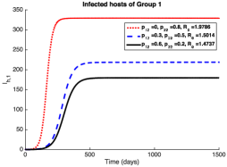
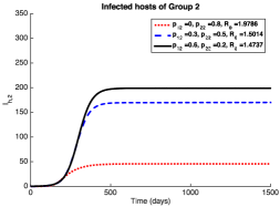
Refer to caption
(a) The level of prevalence of host of group 1 seems to decrease as p12subscript𝑝12p_{12} increases (and hence p11subscript𝑝11p_{11} decreases).
Refer to caption
(b) The level of prevalence of host of group 2 seems to decrease with respect to p22subscript𝑝22p_{22}.
Figure 2: Dynamics of Ih,1subscript𝐼1I_{h,1} and Ih,2subscript𝐼2I_{h,2} for different values of pijsubscript𝑝𝑖𝑗p_{ij}.

Figure 2 displays the dynamics of infected hosts of Group 1 (Fig 2(a)) and Group 2 (Fig 2(b)). The level of endemicity of individuals of Group 1 seems to decrease as proportion of time in Patch 2 (p12subscript𝑝12p_{12}) increases; probably because as p12subscript𝑝12p_{12} increases, p11subscript𝑝11p_{11} decreases. In other words, individuals of Group 1 spend more time in the less riskier Patch 2 (a2=0.4subscript𝑎20.4a_{2}=0.4) than in the riskier Patch 1 (a1=0.5subscript𝑎10.5a_{1}=0.5). We see that the less time that individuals spend in riskier environment the less likely that they will become infected, as one would expect.

In Figure 2(b), the level of endemicity of hosts in Group 2 seems to decrease as p22subscript𝑝22p_{22} increases or equivalently as p21subscript𝑝21p_{21} decreases ( p21+p22+p23=1subscript𝑝21subscript𝑝22subscript𝑝231p_{21}+p_{22}+p_{23}=1 and p23subscript𝑝23p_{23} is fixed). It is so because individuals are increasing their residence time in Patch 2 (a2=0.4subscript𝑎20.4a_{2}=0.4) rather than in Patch 1.

Refer to caption
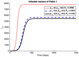
(a) The level of prevalence of vectors of Patch 1 is decreasing as p12subscript𝑝12p_{12} increases and p22subscript𝑝22p_{22} increases.
Refer to caption
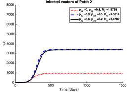
(b) The level of prevalence of host of group 2
Figure 3: Dynamics of Iv,1subscript𝐼𝑣1I_{v,1} and Iv,2subscript𝐼𝑣2I_{v,2} for different values of pijsubscript𝑝𝑖𝑗p_{ij}.

Figures 3 and 4 offer an overview on how the dynamics of vectors change as the proportion of time that individuals of Group 1 and Group 2 spend in environments 1, 2 and 3 varies. For the selected residence times matrix entries, the prevalence of vector in environment 1 (see Fig 3(a)) is at its highest if p12=0subscript𝑝120p_{12}=0 and p22=0.8subscript𝑝220.8p_{22}=0.8. With this configuration, p11=0.9subscript𝑝110.9p_{11}=0.9 and Patch 1 has the highest effective population size. Moreover, Patch 1 has the highest biting rate, leading to high level of vector infections in that patch.

Though Λv,1=Λv,2subscriptΛ𝑣1subscriptΛ𝑣2\Lambda_{v,1}=\Lambda_{v,2}, the prevalence of vectors Patch 2 (Fig 3(b)) is lower than of Patch 1 (Fig 3(a)), regardless of the combination of the chosen residence times entries. This is because the effective population of Patch 2 is less than the effective population of Patch 1 for all the three selected residence time configurations and also because a1>a2subscript𝑎1subscript𝑎2a_{1}>a_{2}.

Refer to caption
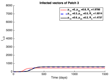
Figure 4: Dynamics of vectors in Patch 3 (Iv,3subscript𝐼𝑣3I_{v,3}) for different values of pijsubscript𝑝𝑖𝑗p_{ij}.

Figure 4 represent the dynamics of the vectors in Patch 3. The number of infected vector in this patch is much less when compared to the number of infected in Patch 1 and 2. Again, the effective population size of Patch 3, with p13=0.1subscript𝑝130.1p_{13}=0.1 and p23=0.2subscript𝑝230.2p_{23}=0.2, is much less when compared to those in Patch 1 and Patch 2. Additionally, we also have by assumption that a3<a2<a1subscript𝑎3subscript𝑎2subscript𝑎1a_{3}<a_{2}<a_{1}.

For the vectors’ prevalence, we obtain similar results as in Fig (3) and Fig (4) even if when biting rates are equal in all the three patches. This last comment highlights the role of the effective population per patch.

Remark 4.1.
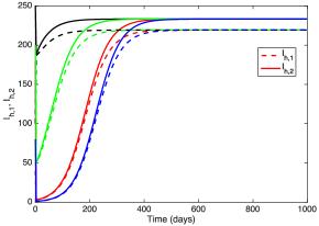
For all the selected combination of the residence times matrix entries in Fig 2-3-4, the matrices MvhMhvsubscript𝑀𝑣subscript𝑀𝑣M_{vh}M_{hv} and MhvMvhsubscript𝑀𝑣subscript𝑀𝑣M_{hv}M_{vh} are irreducible and 0>1subscript01\mathcal{R}_{0}>1 and so the curves of the infected hosts and vectors in those figures are reaching an endemic equilibrium level in accordance with Theorem 2.2.

Refer to caption
(a) Dynamics of infected hosts of Group 1 and Group 2.
Refer to caption
(b) Dynamics of infected vectors of Patch 1 and Patch 2.
Figure 5: Trajectories of System (5), with n=2𝑛2n=2 groups and m=3𝑚3m=3 patches with 4 different initial conditions. The trajectories are converging toward a unique interior endemic equilibrium.

In Figure 5 and 6, we consider the case where the residence time matrix is fixed as follows:

=(0.40.30.30.40.40.2)0.40.30.30.40.40.2\mathbb{P}=\left(\begin{array}[]{ccc}0.4&0.3&0.3\\ 0.4&0.4&0.2\end{array}\right)

In that case, the matrices MhvMvhsubscript𝑀𝑣subscript𝑀𝑣M_{hv}M_{vh} and MvhMhvsubscript𝑀𝑣subscript𝑀𝑣M_{vh}M_{hv} are both irreducible. We sketch the trajectories of System (5) for different initial conditions. Since, with these values of parameters and residence times matrix, the basic reproduction number is 0(3,2)=1.4771subscript0321.4771\mathcal{R}_{0}(3,2)=1.4771, and so the result of Theorem 2.2 should hold and Figure 5 confirms that. More precisely, Figure 5(a) shows that the trajectories of infected individuals of Group 1 and Group 2 converge to the same interior endemic equilibrium for four different initial conditions, namely IC1=[Ih,1(0)=180,Ih,2(0)=180,Iv,1(0)=0,Iv,2(0)=0,Iv,3(0)=0]𝐼subscript𝐶1delimited-[]formulae-sequencesubscript𝐼10180formulae-sequencesubscript𝐼20180formulae-sequencesubscript𝐼𝑣100formulae-sequencesubscript𝐼𝑣200subscript𝐼𝑣300IC_{1}=[I_{h,1}(0)=180,\;I_{h,2}(0)=180,\;I_{v,1}(0)=0,\;I_{v,2}(0)=0,\;I_{v,3}(0)=0] (solid red for Ih,1subscript𝐼1I_{h,1} and dashed red for Ih,2subscript𝐼2I_{h,2} in Fig 5(a).), IC2=[Ih,1(0)=100,Ih,2(0)=250,Iv,1(0)=6000,Iv,2(0)=1000,Iv,3(0)=200]𝐼subscript𝐶2delimited-[]formulae-sequencesubscript𝐼10100formulae-sequencesubscript𝐼20250formulae-sequencesubscript𝐼𝑣106000formulae-sequencesubscript𝐼𝑣201000subscript𝐼𝑣30200IC_{2}=[I_{h,1}(0)=100,\;I_{h,2}(0)=250,\;I_{v,1}(0)=6000,\;I_{v,2}(0)=1000,\;I_{v,3}(0)=200] (solid black for Ih,1subscript𝐼1I_{h,1} and dotted black for Ih,2subscript𝐼2I_{h,2} in 5(a).), IC3=[Ih,1(0)=80,Ih,2(0)=200,Iv,1(0)=1000,Iv,2(0)=500,Iv,3(0)=400]𝐼subscript𝐶3delimited-[]formulae-sequencesubscript𝐼1080formulae-sequencesubscript𝐼20200formulae-sequencesubscript𝐼𝑣101000formulae-sequencesubscript𝐼𝑣20500subscript𝐼𝑣30400IC_{3}=[I_{h,1}(0)=80,\;I_{h,2}(0)=200,\;I_{v,1}(0)=1000,\;I_{v,2}(0)=500,\;I_{v,3}(0)=400] (solid green for Ih,1subscript𝐼1I_{h,1} and dotted green for Ih,2subscript𝐼2I_{h,2} in 5(a).) and IC4=[Ih,1(0)=40,Ih,2(0)=80,Iv,1(0)=1,Iv,2(0)=2,Iv,3(0)=3]𝐼subscript𝐶4delimited-[]formulae-sequencesubscript𝐼1040formulae-sequencesubscript𝐼2080formulae-sequencesubscript𝐼𝑣101formulae-sequencesubscript𝐼𝑣202subscript𝐼𝑣303IC_{4}=[I_{h,1}(0)=40,\;I_{h,2}(0)=80,\;I_{v,1}(0)=1,\;I_{v,2}(0)=2,\;I_{v,3}(0)=3] (solid blue for Ih,1subscript𝐼1I_{h,1} and dotted blue for Ih,2subscript𝐼2I_{h,2} in 5(a).).
Similarly, Figure 5(b) displays the trajectories of infected vectors in the three considered environments. For all the above-mentioned initial conditions, these trajectories converge to their interior endemic equilibrium level.
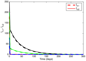
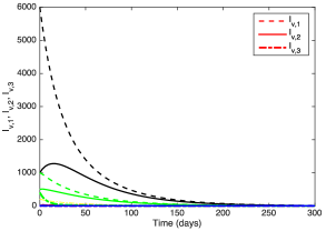
Refer to caption
(a) Dynamics of infected hosts of Group 1 and Group 2.
Refer to caption
(b) Dynamics of infected vectors of Patch 1 and Patch 2.
Figure 6: Trajectories of System (5), with n=2𝑛2n=2 groups and m=3𝑚3m=3 Patches with 4 different initial conditions. With βhv=0.2subscript𝛽𝑣0.2\beta_{hv}=0.2 and βvh=0.4subscript𝛽𝑣0.4\beta_{vh}=0.4, we have have 0(3,2)=0.6353subscript0320.6353\mathcal{R}_{0}(3,2)=0.6353 and the trajectories are converging toward the disease free equilibrium.

Figure 6 sketches the case where the values of all the parameters are the same as above but where βhv=0.2subscript𝛽𝑣0.2\beta_{hv}=0.2 and βvh=0.4subscript𝛽𝑣0.4\beta_{vh}=0.4. In this case, the basic reproduction number is 0=0.6353subscript00.6353\mathcal{R}_{0}=0.6353 which is less than one. As we can see in Fig 6(a) and 6(b), the trajectories of infected hosts of the two groups and the infected vectors of the three patches are converging to zero for the above four initial conditions. This suggests that the DFE is globally asymptotically stable and confirms the result of Theorem 2.1.

Now, we consider the case where the configuration of the Group-Patch network is not irreducible. If we assume that p12=p21=p23=0subscript𝑝12subscript𝑝21subscript𝑝230p_{12}=p_{21}=p_{23}=0, the residence times matrix becomes

=(0.700.3010).0.700.3010\mathbb{P}=\left(\begin{array}[]{ccc}0.7&0&0.3\\ 0&1&0\end{array}\right).

This imply that Mhv=(a1βvhN¯v,1Nh,1(μ1+γ1)00a2βvhN¯v,2Nh,2(μ2+γ2)a3βvhN¯v,3Nh,1(μ1+γ1)0)subscript𝑀𝑣subscript𝑎1subscript𝛽𝑣subscript¯𝑁𝑣1subscript𝑁1subscript𝜇1subscript𝛾100subscript𝑎2subscript𝛽𝑣subscript¯𝑁𝑣2subscript𝑁2subscript𝜇2subscript𝛾2subscript𝑎3subscript𝛽𝑣subscript¯𝑁𝑣3subscript𝑁1subscript𝜇1subscript𝛾10M_{hv}=\left(\begin{array}[]{cc}\frac{a_{1}\beta_{vh}\bar{N}_{v,1}}{N_{h,1}(\mu_{1}+\gamma_{1})}&0\\ 0&\frac{a_{2}\beta_{vh}\bar{N}_{v,2}}{N_{h,2}(\mu_{2}+\gamma_{2})}\\ \frac{a_{3}\beta_{vh}\bar{N}_{v,3}}{N_{h,1}(\mu_{1}+\gamma_{1})}&0\end{array}\right) and Mvh=(a1βhvμv+δ10a3βhvμv+δ30a2βhvμv+δ20)subscript𝑀𝑣subscript𝑎1subscript𝛽𝑣subscript𝜇𝑣subscript𝛿10subscript𝑎3subscript𝛽𝑣subscript𝜇𝑣subscript𝛿30subscript𝑎2subscript𝛽𝑣subscript𝜇𝑣subscript𝛿20M_{vh}=\left(\begin{array}[]{ccc}\frac{a_{1}\beta_{hv}}{\mu_{v}+\delta_{1}}&0&\frac{a_{3}\beta_{hv}}{\mu_{v}+\delta_{3}}\\ 0&\frac{a_{2}\beta_{hv}}{\mu_{v}+\delta_{2}}&0\end{array}\right). Hence, the matrices MvhMhvsubscript𝑀𝑣subscript𝑀𝑣M_{vh}M_{hv} and MhvMvhsubscript𝑀𝑣subscript𝑀𝑣M_{hv}M_{vh} are not both irreducible and hence Theorem 2.2 does not hold, as shown in Fig 7, where a boundary equilibrium appears. In this case, members of Group 2 spend all their time in Patch 2 and hence are isolated from the rest of groups and patches. The basic reproduction number of Group 2 in Patch 2 is (0(2,2))2=a22βvhβhvNv,2(μv+δ2)(μ2+γ2)Nh,2=0.8superscriptsubscript0222superscriptsubscript𝑎22subscript𝛽𝑣subscript𝛽𝑣subscript𝑁𝑣2subscript𝜇𝑣subscript𝛿2subscript𝜇2subscript𝛾2subscript𝑁20.8(\mathcal{R}_{0}(2,2))^{2}=\frac{a_{2}^{2}\beta_{vh}\beta_{hv}N_{v,2}}{(\mu_{v}+\delta_{2})(\mu_{2}+\gamma_{2})N_{h,2}}=0.8. The diseases dies out from the hosts of Group 2 (see 7(a), solid curves) and vectors of Patch 2 (7(b), solid curves). Members of Group 1 are connected to Patch 1 and Patch 3. Hence, the corresponding basic reproduction number is (01,1,3)2=a12βvhβhvNv,21(μv+δ1)(μ1+γ1)Nh,1+a32βvhβhvNv,3(μv+δ3)(μ1+γ1)Nh,1=1.8549superscriptsuperscriptsubscript01132superscriptsubscript𝑎12subscript𝛽𝑣subscript𝛽𝑣subscript𝑁𝑣21subscript𝜇𝑣subscript𝛿1subscript𝜇1subscript𝛾1subscript𝑁1superscriptsubscript𝑎32subscript𝛽𝑣subscript𝛽𝑣subscript𝑁𝑣3subscript𝜇𝑣subscript𝛿3subscript𝜇1subscript𝛾1subscript𝑁11.8549(\mathcal{R}_{0}^{1,{1,3}})^{2}=\frac{a_{1}^{2}\beta_{vh}\beta_{hv}N_{v,21}}{(\mu_{v}+\delta_{1})(\mu_{1}+\gamma_{1})N_{h,1}}+\frac{a_{3}^{2}\beta_{vh}\beta_{hv}N_{v,3}}{(\mu_{v}+\delta_{3})(\mu_{1}+\gamma_{1})N_{h,1}}=1.8549. Hence, the disease persists among the members of Group 1(see 7(a), dashed curves) and vectors of Patch 1 and 3 (see 7(b), dashed curves). This case offers a glimpse on how disease dynamics when some groups are strongly connected to some environments while other groups are isolated.
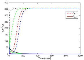
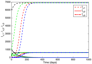
Refer to caption
(a) Dynamics of infected hosts of Group 1 and Group 2.
Refer to caption
(b) Dynamics of infected vectors of Patch 1, Patch 2 and Patch 3.
Figure 7: Trajectories of System (5), with n=2𝑛2n=2 groups and m=3𝑚3m=3 patches with 4 different initial conditions. The disease dies out for the host of Group 2 whereas it persists for those of Group 1. Similarly, the disease dies out for the vector of Patch 2 but persists for the vectors of Patch 1 and 3.

5 Conclusion and discussion

Modeling vector-borne interactions have often been based on well-mixed models that make it difficult to address effectively the role of host mobility on vector borne disease dynamics. Here, we consider a Lagrangian framework where hosts’ dispersal is modeled via the proportion of time that individuals spend in different environments. In the process, we are forced to account, for time variations in effective population size within each patch/environment. The kind of natural adjustment that can significantly alter the quantitative and qualitative dynamics of vector borne dynamics in geographically heterogeneous system; here within spatial scales that make it possible to neglect vector mobility.

And so, we consider a general SIS𝑆𝐼𝑆SIS framework to account for the host dynamics and an SI𝑆𝐼SI framework to account for the vector dynamics. The transmission terms must make adjustments to account for the effective population size generated by the residence time matrix. This is handled via the use of a modified frequency-dependent incidence model that accounts for the effective density of infected hosts within each patch at any time. We compute the basic reproduction number 02(,m,n)superscriptsubscript02𝑚𝑛\mathcal{R}_{0}^{2}(\mathbb{P},m,n) for the general host-vector model and prove that the disease free equilibrium is globally asymptotically stable (GAS) if 02(,m,n)1superscriptsubscript02𝑚𝑛1\mathcal{R}_{0}^{2}(\mathbb{P},m,n)\leq 1. We also show that there exists a unique interior endemic equilibrium that is GAS whenever 02(,m,n)>1superscriptsubscript02𝑚𝑛1\mathcal{R}_{0}^{2}(\mathbb{P},m,n)>1 in the irreducible case, that is, when the hosts’ groups and vector patches are strongly connected. When irreducibility does not hold, the existence of boundary equilibria is identified. In addition, we provide explicit expression for the basic reproduction number whenever the residence time matrix \mathbb{P} is of rank one. Finally, we briefly explore the role of variability in the number of patches and groups on the basic reproduction number, 02(,m,n)superscriptsubscript02𝑚𝑛\mathcal{R}_{0}^{2}(\mathbb{P},m,n) and in the process, bounds for 02(,m,n)superscriptsubscript02𝑚𝑛\mathcal{R}_{0}^{2}(\mathbb{P},m,n) are identified.

Our results generalize those of [18, 42, 58] since our models account for the time-dependant effective patch population size. The approach we considered here includes the case where the hosts’ structure is defined by residency ( see Subsection 4.1) as well as the case when the hosts’ structure is defined by groups or classes that are independent from the spatially explicit patches.

In short, the contributions of this manuscript are primarily tied to the effective population size, a function of the mobility matrix =(pij)1in,1jmsubscriptsubscript𝑝𝑖𝑗1𝑖𝑛1𝑗𝑚\mathbb{P}=(p_{ij})_{\begin{subarray}{c}1\leq i\leq n,\\ 1\leq j\leq m\end{subarray}}, where the pijsubscript𝑝𝑖𝑗p_{ij} denotes the proportion of time the host of group i𝑖i (or the member of a well defined class i𝑖i) spends in environment j𝑗j. We explicitly study the role of the matrix \mathbb{P} on 0subscript0\mathcal{R}_{0} and connected the dynamics to the reducibility and irreducibility structure of the system. Theorems were established and examples provided on the role of pachiness and groupness on the disease dynamics.

Acknowledgements

We are grateful to the handling editor and two anonymous reviewers for their helpful comments and suggestions which led to an improvement of this paper. C.C.C is supported in part grant #1R01GM100471-01 from the National Institute of General Medical Sciences (NIGMS) at the National Institutes of Health. The contents of this manuscript are solely the responsibility of the authors and do not necessarily represent the official views of DHS or NIGMS. The funders had no role in study design, data collection and analysis, decision to publish, or preparation of the manuscript.

References

  • [1] B. Adams and D. D. Kapan, Man bites mosquito: understanding the contribution of human movement to vector-borne disease dynamics, PloS One, 4 (2009).
  • [2] J. Arino, C. Bowman, A. Gumel, and S. Portet, Effect of pathogen-resistant vectors on the transmission dynamics of a vector-borne disease., J Biol. Dynamics, 1 (2007), pp. 320–346.
  • [3] J. Arino, A. Ducrot, and P. Zongo, A metapopulation model for malaria with transmission-blocking partial immunity in hosts, Journal of mathematical biology, 64 (2012), pp. 423–448.
  • [4] J. L. Aron and R. M. May, The population dynamics of malaria, in The population dynamics of infectious diseases: theory and applications, Springer, 1982, pp. 139–179.
  • [5] P. Auger, E. Kouokam, G. Sallet, M. Tchuente, and B. Tsanou, The ross-macdonald model in a patchy environment, Math. Biosci., 216 (2008), pp. 123–131.
  • [6] N. T. Bailey et al., The biomathematics of malaria. the biomathematics of diseases: 1., The biomathematics of malaria. The Biomathematics of Diseases: 1., (1982).
  • [7] D. Bichara, Y. Kang, C. Castillo-Chavez, R. Horan, and C. Perrings, Sis and sir epidemic models under virtual dispersal, arXiv preprint arXiv:1503.08881, (2015).
  • [8] R. Biritwum, J. Welbeck, and G. Barnish, Incidence and management of malaria in two communities of different socio–economic level, in accra, ghana, Annals of tropical medicine and parasitology, 94 (2000), pp. 771–778.
  • [9] D. D. Bonnet and D. J. Worcester, The dispersal of aedes albopictus in the territory of hawaii, The American journal of tropical medicine and hygiene, 1 (1946), pp. 465–476.
  • [10] C. Castillo-Chavez, R. Curtiss, P. Daszak, S. A. Levin, O. Patterson-Lomba, C. Perrings, G. Poste, and S. Towers, Beyond ebola: lessons to mitigate future pandemics, The Lancet Global Health, 3 (2015), pp. e354–e355.
  • [11] C. Castillo-Chavez, B. Song, and J. Zhangi, An epidemic model with virtual mass transportation: The case of smallpox, Bioterrorism: Mathematical Modeling Applications in Homeland Security, 28 (2003), p. 173.
  • [12] C. Castillo-Chavez and H. R. Thieme, Asymptotically autonomous epidemic models, in Mathematical Population Dynamics: Analysis of Heterogeneity, Volume One: Theory of Epidemics,, O. Arino, A. D.E., and M. Kimmel, eds., Wuerz, 1995.
  • [13] C. Castillo-Chavez, J. X. Velasco-Hernandez, and S. Fridman, Modeling contact structures in biology, in Frontiers in Mathematical Biology, S. A. Levin, ed., vol. 100, Springer, 1994, pp. 454–491.
  • [14] N. Chitnis, Using Mathematical models in controlling the spread of malaria, PhD thesis, University of Arizona, 2005.
  • [15] N. Chitnis, J. M. Cushing, and J. M. Hyman, Bifurcation analysis of a mathematical model for malaria transmission, SIAM J. Appl. Math., 67 (2006), pp. 24–45 (electronic).
  • [16] N. Chitnis, J. M. Hyman, and J. Cushing, Determining Important Parameters in the Spread of Malaria Through the Sensitivity Analysis of a Mathematical Model, Bull. Math. Biol., (2008).
  • [17] N. Chitnis, J. M. Hyman, and C. A. Manore, Modelling vertical transmission in vector-borne diseases with applications to rift valley fever, Journal of biological dynamics, 7 (2013), pp. 11–40.
  • [18] C. Cosner, J. Beier, R. Cantrell, D. Impoinvil, L. Kapitanski, M. Potts, A. Troyo, and S. Ruan, The effects of human movement on the persistence of vector-borne diseases, Journal of theoretical biology, 258 (2009), pp. 550–560.
  • [19] O. Diekmann, J. A. P. Heesterbeek, and J. A. J. Metz, On the definition and the computation of the basic reproduction ratio R0subscript𝑅0R_{0} in models for infectious diseases in heterogeneous populations, J. Math. Biol., 28 (1990), pp. 365–382.
  • [20] K. Dietz, transmission and control of arbovirus diseases, in SIMS 1974 Utah conference proceedings, D. Ludwig and K. Cooke, eds., 1975, pp. 104–121.
  • [21]  , Epidemiologic interference of virus population, J. Math. Biol., 8 (1979), pp. 291–300.
  • [22]  , Models for vector-borne parasitic diseases, in Vito Volterra Symposium on Mathematical Models in Biology (Rome, 1979), vol. 39 of Lecture Notes in Biomath., Springer, Berlin, 1980, pp. 264–277.
  • [23] Y. Dumont and F. Chiroleu, Vector control for the chikungunya disease, Math. Biosci. Eng, 7 (2010), pp. 313–345.
  • [24] Y. Dumont, F. Chiroleu, and C. Domerg, On a temporal model for the chikungunya disease: modeling, theory and numerics, Mathematical biosciences, 213 (2008), pp. 80–91.
  • [25] C. Dye and G. Hasibeder, Population dynamics of mosquito-borne disease: effects of flies which bite some people more frequently than others, Transactions of the Royal Society of Tropical Medicine and Hygiene, 80 (1986), pp. 69–77.
  • [26] A. Elbers, C. Koenraadt, and R. Meiswinkel, Mosquitoes and culicoides biting midges: vector range and the influence of climate change, Rev. Sci. Tech. Off. Int. Epiz, 34 (2015), pp. 123–137.
  • [27] F. Forouzannia and A. B. Gumel, Mathematical analysis of an age-structured model for malaria transmission dynamics, Mathematical biosciences, 247 (2014), pp. 80–94.
  • [28] D. Gao and S. Ruan, An sis patch model with variable transmission coefficients, Mathematical biosciences, 232 (2011), pp. 110–115.
  • [29]  , A multipatch malaria model with logistic growth populations, SIAM journal on applied mathematics, 72 (2012), pp. 819–841.
  • [30] S. M. Garba, A. B. Gumel, and M. A. Bakar, Backward bifurcations in dengue transmission dynamics, Mathematical biosciences, 215 (2008), pp. 11–25.
  • [31] D. Grünbaum, Translating stochastic density-dependent individual behavior with sensory constraints to an eulerian model of animal swarming, Journal of mathematical biology, 33 (1994), pp. 139–161.
  • [32] H. Guo, M. Li, and Z. Shuai, Global stability of the endemic equilibrium of multigroup models., Can. Appl. Math. Q., 14 (2006), pp. 259–284.
  • [33] G. Hasibeder and C. Dye, Population dynamics of mosquito-borne disease: persistence in a completely heterogeneous environment, Theoretical population biology, 33 (1988), pp. 31–53.
  • [34] M. Hirsch, The dynamical system approach to differential equations, Bull. AMS, 11 (1984), pp. 1–64.
  • [35] N. A. Honório, W. d. C. Silva, P. J. Leite, J. M. Gonçalves, L. P. Lounibos, and R. Lourenço-de Oliveira, Dispersal of aedes aegypti and aedes albopictus (diptera: Culicidae) in an urban endemic dengue area in the state of rio de janeiro, brazil, Memórias do Instituto Oswaldo Cruz, 98 (2003), pp. 191–198.
  • [36] A. Iggidr, G. Sallet, and M. O. Souza, On the dynamics of a class of multi-group models for vector-borne diseases, arXiv preprint arXiv:1409.1470, (2014).
  • [37] A. Iggidr, G. Sallet, and B. Tsanou, Global stability analysis of a metapopulation sis epidemic model, Mathematical Population Studies, 19 (2012), pp. 115–129.
  • [38] C. Kaufmann and H. Briegel, Flight performance of the malaria vectors anopheles gambiae and anopheles atroparvus, Journal of vector ecology, 29 (2004), pp. 140–153.
  • [39] K. Koram, S. Bennett, J. Adiamah, and B. Greenwood, Socio-economic risk factors for malaria in a peri-urban area of the gambia, Transactions of the royal society of tropical medicine and hygiene, 89 (1995), pp. 146–150.
  • [40] T. Kuniya and Y. Muroya, Global stability of a multi-group sis epidemic model for population migration., Discrete & Continuous Dynamical Systems-Series B, 19 (2014).
  • [41] G. Kuno, Review of the factors modulating dengue transmission, Epidemiologic reviews, 17 (1995), pp. 321–335.
  • [42] S. Lee and C. Castillo-Chavez, The role of residence times in two-patch dengue transmission dynamics and optimal strategies, Journal of theoretical biology, 374 (2015), pp. 152–164.
  • [43] G. Macdonald, Epidemiological basis of malaria control, Bulletin of the World Health Organization, 15 (1956), p. 613.
  • [44] G. Macdonald, Theory of the eradication of malaria, Bulletin of the World Health Organization, 15 (1956), p. 369.
  • [45] G. Macdonald et al., The epidemiology and control of malaria., The Epidemiology and Control of Malaria., (1957).
  • [46] P. Martens and L. Hall, Malaria on the move: human population movement and malaria transmission., Emerging infectious diseases, 6 (2000), p. 103.
  • [47] A. G. Ngwa, On the Population Dynamics of the Malaria Vector, Bull Math Biol, (2006).
  • [48] A. G. Ngwa and W. Shu, A mathematical model for Endemic Malaria with Variable Human and Mosquito Population, Math. Comput. Modelling, 32 (2000), pp. 747–763.
  • [49] M. Niebylski and G. Craig Jr, Dispersal and survival of aedes albopictus at a scrap tire yard in missouri., Journal of the American Mosquito Control Association, 10 (1994), pp. 339–343.
  • [50] R. Novak, A north american model to contain the spread of aedes albopictus through tire legislation., Parassitologia, 37 (1995), pp. 129–139.
  • [51] A. Okubo, Diffusion and ecological problems: Mathematical models, Biomathematics, 10 (1980).
  • [52] A. Okubo and S. A. Levin, Diffusion and ecological problems: modern perspectives, vol. 14, Springer Science & Business Media, 2013.
  • [53] O. Onwujekwe, B. Uzochukwu, S. Eze, E. Obikeze, C. Okoli, and O. Ochonma, Improving equity in malaria treatment: relationship of socio-economic status with health seeking as well as with perceptions of ease of using the services of different providers for the treatment of malaria in nigeria, Malar J, 7 (2008), pp. 1–10.
  • [54] W. H. Organization, Dengue control, World Health Organization, (September 23, 2015). http://www.who.int/denguecontrol/mosquito/en/.
  • [55] W. H. Organization et al., A global brief on vector-borne diseases, World Health Organization, (2014). http://www.who.int/campaigns/world-health-day/2014/global-brief/en/.
  • [56] C. Perrings, C. Castillo-Chavez, G. Chowell, P. Daszak, E. P. Fenichel, D. Finnoff, R. D. Horan, A. M. Kilpatrick, A. P. Kinzig, N. V. Kuminoff, et al., Merging economics and epidemiology to improve the prediction and management of infectious disease, EcoHealth, 11 (2014), pp. 464–475.
  • [57] P. Reiter, Climate change and mosquito-borne disease: knowing the horse before hitching the cart, Revue scientifique et technique-Office international des épizooties, 27 (2014).
  • [58] D. J. Rodríguez and L. Torres-Sorando, Models of infectious diseases in spatially heterogeneous environments, Bulletin of Mathematical Biology, 63 (2001), pp. 547–571.
  • [59] D. Roiz, R. Eritja, R. Escosa, J. Lucientes, E. Marques, R. Melero-Alcibar, S. Ruiz, and R. Molina, A survey of mosquitoes breeding in used tires in spain for the detection of imported potential vector species, Journal of Vector Ecology, 32 (2007), pp. 10–15.
  • [60] R. Ross, The prevention of malaria, John Murray, 1911.
  • [61] R. Ross, An application of the theory of probabilities to the study of a priori pathometry. part i, Proc. R. Soc. Lond. A, 92 (1916), pp. 204–230.
  • [62] R. Ross and H. Hudson, An application of the theory of probabilities to the study of a priori pathometry. part ii, Proc. R. Soc. Lond. A, 93 (1917), pp. 212–225.
  • [63] R. Ross and H. Hudson, An application of the theory of probabilities to the study of a priori pathometry. part iii, Proc. R. Soc. Lond. A, 93 (1917), pp. 225–240.
  • [64] N. W. Ruktanonchai, D. L. Smith, and P. De Leenheer, Parasite sources and sinks in a patched ross-macdonald malaria model with human and mosquito movement: implications for control, Mathematical Biosciences, 279 (2016), pp. 90–101.
  • [65] D. L. Smith, J. Dushoff, and F. E. McKenzie, The risk of a mosquito-borne infection in a heterogeneous environment, PLoS biology, 2 (2004), p. e368.
  • [66] H. Smith, Cooperative systems of differential equations with concave nonlinearities, Nonlinear Analysis: Theory, Methods & Applications, 10 (1986), pp. 1037–1052.
  • [67] M. P. Stürchler, The vector and measures against mosquito bites, in Travelers’ Malaria, P. Schlagenhauf-Lawlor, ed., BC Decker, 2001, ch. 8, pp. 88–105.
  • [68] M. M. Thiboutot, S. Kannan, O. U. Kawalekar, D. J. Shedlock, A. S. Khan, G. Sarangan, P. Srikanth, D. B. Weiner, and K. Muthumani, Chikungunya: a potentially emerging epidemic, PLoS Negl Trop Dis, 4 (2010), p. e623.
  • [69] M. A. Tolle, Mosquito-borne diseases, Current problems in pediatric and adolescent health care, 39 (2009), pp. 97–140.
  • [70] L. Torres-Sorando and D. J. Rodrìguez, Models of spatio-temporal dynamics in malaria, Ecological modelling, 104 (1997), pp. 231–240.
  • [71] P. van den Driessche and J. Watmough, reproduction numbers and sub-threshold endemic equilibria for compartmental models of disease transmission, Math. Biosci., 180 (2002), pp. 29–48.
  • [72] M. Vidyasagar, Decomposition techniques for large-scale systems with nonadditive interactions: Stability and stabilizability., IEEE Trans. Autom. Control, 25 (1980), pp. 773–779.
  • [73] Y. Xiao and X. Zou, Transmission dynamics for vector-borne diseases in a patchy environment, Journal of mathematical biology, 69 (2014), pp. 113–146.