Bayesian model averaging: A systematic review and conceptual classification

Abstract

Bayesian Model Averaging (BMA) is an application of Bayesian inference to the problems of model selection, combined estimation and prediction that produces a straightforward model choice criteria and less risky predictions. However, the application of BMA is not always straightforward, leading to diverse assumptions and situational choices on its different aspects. Despite the widespread application of BMA in the literature, there were not many accounts of these differences and trends besides a few landmark revisions in the late $1990$s and early $2000$s, therefore not taking into account any advancements made in the last $15$ years. In this work, we present an account of these developments through a careful content analysis of $587$ articles in BMA published between $1996$ and $2014$. We also develop a conceptual classification scheme to better describe this vast literature, understand its trends and future directions and provide guidance for the researcher interested in both the application and development of the methodology. The results of the classification scheme and content review are then used to discuss the present and future of the BMA literature.

math.PR/0000000

T1AMS 1991 subject classifications: 62F15; 62C10; key words and phrases: Bayesian Model Averaging; Systematic review; Conceptual classification scheme; Qualitative content analysis

and

t2To whom correspondence should be addressed. This work was partially funded by the Brazilian’s Ministry of Education Coordenação de Aperfeiçoamento de Pessoal de Nível Superior (CAPES) through a postdoctoral PNPD research grant

1 Introduction

It is very common in practice that multiple models provide adequate descriptions of the distributions generating the observed data. It is standard statistical practice that, in such situations, a better model must be selected according to some criteria, like model fit to the observed dataset, predictive capabilities or likelihood penalizations such as information criteria. After selection is performed, all inference is made and conclusions drawn assuming the selected model as the true model.

However, there are downsides to this approach. The selection of one particular model may lead to overconfident inferences and riskier decision making as it ignores the existent model uncertainty in favor of very particular distributions and assumptions on the model of choice. Therefore, modeling this source of uncertainty to appropriately select or combine multiple models is very desirable.

Using Bayesian inference to this purpose has been suggested as a framework capable of achieving these goals (Leamer, 1978). Bayesian Model Averaging (BMA) is an extension of the usual Bayesian inference methods in which one does not only models parameter uncertainty through the prior distribution, but also model uncertainty obtaining posterior parameter and model posteriors using Bayes’ theorem and therefore allowing for allow for direct model selection, combined estimation and prediction.

1.1 Background

Let each model in consideration be denoted by $M_{l}$, $l=1,\ldots,K$ representing a set of probability distributions encompassing the likelihood function $L(\boldsymbol{Y}|\theta_{l},M_{l})$ of the observed data $\boldsymbol{Y}$ in terms of model specific parameters $\theta_{l}$ and a set of prior probability densities for said parameters, denoted in general terms by $\pi(\theta_{l}|M_{l})$ on which we omit eventual prior hyperparameters for the sake of clarity. Notice that both the likelihood and priors are conditional on a particular model.

Given a model, one then obtains the posterior distribution using Bayes’ theorem, resulting in

$$\pi(\theta_{l}|\boldsymbol{Y},M_{l})=\frac{L(\boldsymbol{Y}|\theta_{l},M_{l})\pi(\theta_{l}|M_{l})}{\int L(\boldsymbol{Y}|\theta_{l},M_{l})\pi(\theta_{l}|M_{l})d\theta_{l}}$$ (1)

where the integral in the denominator is calculated over the support set for each prior distribution and represents the marginal distribution of the dataset over all parameter values specified in model $M_{l}$.

This quantity is essential for BMA applications as we will show momentarily and is called the model’s marginal likelihood or model evidence and is denoted by

$$\pi(\boldsymbol{Y}|M_{l})=\int L(\boldsymbol{Y}|\theta_{l},M_{l})\pi(\theta_{l}|M_{l})d\theta_{l}$$ (2)

Bayesian model averaging then adds a layer to this hierarchical modeling present in Bayesian inference by assuming a prior distribution over the set of all considered models describing the prior uncertainty over each model’s capability to accurately describe the data. If there is a probability mass function over all the models with values $\pi(M_{l})$ for $l=1,\ldots,K$, then Bayes’ theorem can be used to derive posterior model probabilities given the observed data by

$$\pi(M_{l}|\boldsymbol{Y})=\frac{\pi(\boldsymbol{Y}|M_{l})\pi(M_{l})}{\sum_{m=1}^{K}\pi(\boldsymbol{Y}|M_{m})\pi(M_{m})},$$ (3)

resulting in a straightforward posterior model probability, representing the backing of each considered model by the observed data.

There is also a link between these posterior model probabilities and the use of Bayes Factors. Given two models $l$ and $m$, the Bayes factor of model $l$ against model $m$ is given by

$$BF_{lm}=\frac{\pi(M_{l}|\boldsymbol{Y})}{\pi(M_{m}|\boldsymbol{Y})},$$ (4)

thus quantifying the relative strength of the evidence in favor of model $l$ against that of model $m$. Given a baseline model, which we arbitrarily fix as model $1$, it is clear that equation (3) can be written in terms of Bayes Factors by simply dividing by the baseline model’s evidence, resulting in

$$\pi(M_{l}|\boldsymbol{Y})=\frac{BF_{l1}\pi(M_{l})}{\sum_{m=1}^{K}BF_{m1}\pi(M_{m})},$$ (5)

which means that one can estimate the posterior model probabilities by using estimates for Bayes Factors and vice versa.

These model probabilities can mainly be used for two purposes. First, the posterior probabilities (3) can be used as a straightforward model selection criteria, with the most likely model being selected. Second, consider a quantity of interest $\Delta$ present in all models, such as a covariate or future observation, it follows that its marginal posterior distribution across all models is given by

$$\pi(\Delta|\boldsymbol{Y})=\sum_{l=1}^{K}\pi(\Delta|\boldsymbol{Y},M_{l})\pi(M_{l}|\boldsymbol{Y}),$$ (6)

which is an average of all posterior distributions weighted by each posterior model probability. Therefore, BMA allows for a direct combination of models to obtain combined parameter estimates or predictions (Roberts, 1965). This practice leads to predictions with lower risk under a logarithmic scoring rule (Madigan and Raftery, 1994) than using a single model.

However, the implementation and application of BMA is not without difficulties. A prior distribution over the considered models must be specified, which is non trivial in most applications. Additionally, calculating each model evidence (equation 2) is non-trivial. Except in simple settings like in some generalized linear models with conjugate distributions, the evidence does not present a closed form and must be approximated, which presents plenty of challenges and is an active research field (Friel and Wyse, 2012).

Despite these difficulties, BMA was extensively applied in the last $20$ years, mostly in combining multiple models for predictive purposes and selecting models, particularly covariate sets in regression models or network structure in Bayesian Network models. The latter application induces another pitfall in the form of large model spaces. For instance, consider a regression model with $p$ covariates. The number of possible models without any interaction coefficients is $2^{p}$, which represents a large number of models even for moderate values of $p$. This difficulty can be mostly addressed by prior filtering of all possible models or through stochastic search algorithms over the model space.

1.2 Objectives of this review

As mentioned before, the idea of selecting and combining models based on their posterior probabilities is not news, but a series of advances made in the $1990s$ made the implementation and application of these ideas a reality. Following Leamer (1978), most model selection and marginal probabilities were only obtainable for the linear model under very specific parameter priors. However, the seminal work by Raftery (1996) paved the way for a multitude of applications by providing a straightforward approximation for the evidence in generalized linear models.

There were also advances in the implementation of BMA in large model spaces, from a preliminary filtering based on posterior probability ratios called Occam’s Window (Madigan and Raftery, 1994) to a stochastic search algorithm inspired in the Reversible Chain Markov Chain Monte Carlo (Green, 1995) with trans-dimensional jumps based on posterior model probabilities (the MC³ algorithm Madigan et al. (1995)).

We also noticed that following the landmark reviews of Hoeting et al. (1999) and Wasserman (2000), there were no comprehensive reviews of the developments and applications of BMA in the last $15$ years, which does not account for the developments in Bayesian inference brought by the Markov Chain Monte Carlo revolution in the late $1990$s and $2000$s. With this paper, we aim to cover this undocumented period, specifically we have the following goals:

• To provide a conceptual classification scheme (CCS) to review and classify key components of the BMA literature

• To summarize research findings and identify research trends

• To obtain useful guidance for researchers interested in applying BMA to complex models

1.3 Outline

The remainder of this paper is structured as follows. In Section 2, we outline the literature search procedure and criteria employed to select the relevant BMA literature. The content of each selected article is then classified according to its main features using the Conceptual Classification Scheme described in Section 3, obtaining the patterns we describe and discuss in Section 4. We conclude in Section 5 with some guidance on the directions of the BMA literature.

2 Survey methodology

To better understand how BMA was applied, we chose to perform a content analysis of the published literature. The purpose of a content analysis is to systematically evaluate all forms of a recorded communication, identifying and classifying key contributions to a field and clarify trends, practice and indicate research possibilities. To achieve this objective, we formulated a systematic review following the guidelines in Moher et al. (2009) specifying objective criteria for defining the relevant literature to revise and appropriate ways to report our findings.

2.1 Literature search procedure

Aiming to perform a comprehensive search in the BMA literature, we combined four databases: Elsevier‘s Scopus and ScienceDirect (available at http://www.scopus.com and http://www.sciencedirect.com/ respectively), Thompsom Reuters‘s Web of Science (available at http://apps.webofknowledge.com) and the American Mathematical Society‘s MathSciNet database (available at http://www.ams.org/mathscinet/index.html).

We performed queries of the “Bayesian Model Averaging” term restricted to the $1996-2014$ period on the publications’ title, abstract and keywords for queries in Scopus and ScienceDirect, topic (encompassing title, abstract, keywords and proprietary “keywords plus”) in Web of Science and “Anywhere” in MathSciNet, as it presented fewer search options. The time period was chosen to cover most of the published literature not covered by previous works while still including seminal works.

Two exclusion criteria were employed over search results to select articles for further revision, namely:

1. Search results written in English, published in peer-reviewed journals as an article (which excludes conference proceedings, theses, dissertations, books, etc.) and available online.

2. Articles explicitly employing BMA, therefore excluding articles only listing BMA in keywords, alluding to BMA as a model combination procedure or applying BMA without further explanation or reference to the specific methodology employed.

Articles that did not comply with at least one of the criteria were excluded from the review. The articles were then selected according to the procedure illustrated in Figure 1. Using the aforementioned queries, $841$ articles were found in Scopus, $731$ in Web of Science, $167$ in ScienceDirect and $80$ in MathSciNet. After the removal of duplicates and application of the first exclusion criterion, $703$ articles were listed for further investigation and carefully revised, leading to the exclusion of $116$ articles based on the second exclusion criterion, leaving $587$ articles for classification.

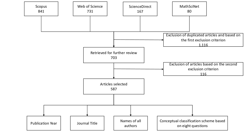
Figure 1: Literature search procedure and number of selected articles

2.2 Structure of the dataset

The final dataset consisting of $587$ eligible articles were then classified according to four main categories:

1. Publication year

2. Names of all authors

3. Journal title

4. Responses to the eight items of the Conceptual Classification Scheme (CCS)

3 A conceptual scheme for BMA

Besides the systematic review of the literature, we also aimed to employ a content analysis of our finding, aiming to provide further inside into the applications of BMA, identify research trends and elucidate possible research directions and opportunities. To achieve this objective, we immersed ourselves in the selected dataset to better define characteristics in which current research that can be used to better understand the literature. This conventional content analysis (Hsieh and Shannon, 2005) allows us to better understand the literature without preconceived notions.

We codified these formulated characteristics into a conceptual classification scheme inspired in the scheme developed in Hachicha and Ghorbel (2012), but adapted to characteristics relevant to the Bayesian Model Averaging literature. We then elaborated a Conceptual Classification Scheme (CCS) to classify the literature and refined the defined categories as we revised all articles. An article’s classification according to the CCS is useful to a researcher interested in the field, as it gives key characteristics on the methodology and formulation, leading to more efficient queries into the developments and applications of BMA. In the present work, we elaborated a CCS with $8$ items which, along with the possible responses can be found in Table 1 and thoroughly described below.

Table 1: List of questions and employed categories for the CCS

1. How is BMA used? 1.1. Model choice 1.2. Combined parameter estimation 1.3. Combined prediction 1.4. Conceptual discussion and methodological improvements 1.5. Review of current methods 2. What is the field of application? 2.1. Statistics and Machine Learning 2.2. Physical sciences and engineering 2.3. Biological and medical sciences 2.4. Economics and humanities 3. How are model prior specified? 3.1. Vague prior 3.2. Used verbatim from the literature 3.3. Elicitated from experts or from the problem 3.4. No explicit use or reference / not applicable 4. How is the evidence estimated? 4.1. Monte Carlo sampling and extensions 4.2. Analytical approximations 4.3. Markov Chain Monte Carlo 4.4. Ratio of densities 5. How do the authors real with high dimensionality? 5.1. Dimensionality reduction 5.2. Stochastic search via Markov Chain Monte Carlo 6. Are Markov Chain Monte Carlo based methods employed? 6.1. Yes 6.2. No 7. Is the method validated through simulation studies? 7.1. Yes 7.2. No 8. Is the application validated through data-driven procedures? 8.1. Cross validation and data splitting 8.2. Leave-one-out or K-fold cross validation 8.3. Posterior predictive checks 8.4. None / not applicable

3.1 Usage

Being a framework for model selection and combination, BMA can be used to solve a wide range of problems. As such, we first classified each eligible article with respect to usage. Our content search resulted in five main categories of BMA usage.

The derivation of posterior model probabilities make BMA a very straightforward model choice method. Said probabilities are easily interpretable under the Bayesian paradigm and the model space can be as wide as necessary and it requires no bookkeeping over the number of parameters or kind of penalty as required by the information criteria methods applied in the statistical literature. We therefore singled out articles that employ BMA as a model choice method.

Using the posterior model probabilities as weights, one can produce estimates averaged over all considered models (equation (6)), that can have a lower overall risk and take model uncertainty into consideration. There are two main kind of estimates. When $\Delta$ in equation (6) represents a parameter that is common to all considered models, one can obtain an averaged model estimate. On the other hand, when $\Delta$ represents a future observation or yet to be collected data point, equation (6) can be used to derive an average prediction. Albeit similar, both applications have distinct uses so we classified articles on its use of BMA to obtain joint estimation and prediction, respectively.

As we previously mentioned, BMA is not as direct to apply. As such, there is a considerable technical literature in theoretical aspects and extensions of BMA. There is also retrospective studies in which BMA or any one of the applications mentioned above are revised in a specific area (model selection methods in economics, for instance) so we classified these articles as conceptual discussions and review articles respectively.

3.2 Field of application

Given the wide array of possible uses, we also classified every selected article according to its field of application. We employed a vague classification of BMA applications for two reasons. First, as stated in Section 1.2, we aim to summarize and point research trends, not perform a detailed taxonomy of BMA usage. Second, as BMA (and Bayesian methods in general) find more penetration into applied research, we lack the expertise to discriminate between subfields. Restricting the present work to a more general view, we defined four fields of application.

An immediate field of application for BMA is the Statistics literature, which is in turn heavily borrowed and borrows upon the Machine Learning literature. Therefore, we classified papers more concerned with statistical modeling, theoretical developments and machine learning applications into a single category. After some pioneering works in the statistical literature, BMA found its way into the Biological and Life Sciences, comprising of the studies in the fields of Medicine, Epidemiology, Biological sciences such as Ecology and others. The seminal revision work by Geweke (1999) introduced BMA to the field of Economics and later on to other Humanities such as Political and Social sciences. After a few years, some works started to appear in the fields of Engineering and Physical sciences such as Meteorology and Physics.

3.3 Model priors

Much of the study in Bayesian methods is concerned with the elicitation of prior distributions, representing the uncertainty in place before any data is observed. Elicitating an appropriate prior is a non-trivial task in any Bayesian setting, and such difficulties are compounded in model averaging since a probability measure for the model space is not obvious in principle, which is probably reflected in the reluctance by many authors to explicitly state their priors. Throughout our review, we encountered four main categories.

One can simply assume prior ignorance about which model is correct through a vague prior (i.e., $\pi(M_{l})\propto 1$, $l=1,2,\ldots,K$), that assumes no model is more likely a priori than any other and let the observed data carry all the information. This is not always desirable and sometimes it is possible to perform some elicitation based on expert opinions or specific characteristics of a particular problem, resulting in elicitated priors.

In the case of elicitated, conjugate or simply convenient priors, sometimes a particular choice spreads through the literature, resulting in subsequent authors that use such priors verbatim, which we classified into a single category of a literature prior. Finally, as mentioned previously a number of authors bypass the problem entirely by neither explicitly stating their model priors nor providing references to clarify their assumptions yet still use BMA in some sense. We classified these cases as “not available” (NA).

3.4 Evidence estimation

The estimation of the marginal likelihood (equation (2)), also known as the model evidence is non-trivial in any general setting since it usually involves complicated multidimensional integrands with sometimes complex support sets that can make the integration unfeasible. As such, many solutions have been proposed, which we classified into five categories.

The integral can be approximated by Monte Carlo methods or extensions such as Importance Sampling. Namely, given an importance probability density $w(\theta)$ defined over the same integration domain of equation (2), the evidence can be approximated by taking $R$ random samples $\theta_{1},\ldots,\theta_{R}$ from the probability distribution determined by $w(\theta)$ and computing the weighted average

$$\widehat{\pi(\boldsymbol{Y}|M_{l})}=\frac{1}{R}\sum^{R}_{r=1}\frac{L(\boldsymbol{Y}|\theta_{r},M_{l})\pi(\theta_{r}|M_{l})}{w(\theta_{r})}$$ (7)

which is guaranteed to converge to the evidence by the Strong Law of Large Numbers. Clearly, the ordinary Monte Carlo approximation can be performed by using the parameter prior as an importance density. Further extensions of this idea exist in the form of Bridge sampling (Gelman and Meng, 1998) and other forms of integration. Relying on the same Monte Carlo framework, we classified these methods into one category,

Still in the spirit of Monte Carlo methods but very distinct in practice, one could also sample from a Markov Chain, using Markov Chain Monte Carlo (MCMC) methods to approximate the evidence. Let $\theta^{(1)}_{l},\ldots,\theta^{(R)}_{l}$ be $R$ posterior samples obtained from a MCMC chain and $w(\theta)$ an importance density as defined previously, then one can use the “Importance Sampling” estimator (Gelfand and Dey, 1994)

$$\widehat{\pi(\boldsymbol{Y}|M_{l})}=\left\{\frac{1}{R}\sum_{r=1}^{R}\frac{w(\theta^{(r)}_{l})}{L(\boldsymbol{Y}|\theta^{(r)}_{l},M_{l})\pi(\theta^{(r)}_{l}|M_{l})}\right\}^{-1},$$ (8)

which is, in turn, a generalization of the harmonic mean estimator of Newton and Raftery (1994) that uses the prior as an importance density. The estimator is shown to converge to the evidence as the sample size increases, but an importance function must be finely tuned to avoid estimators with unbounded variance.

Another flavor of MCMC posterior probability estimator comes through the use of trans-dimensional Markov Chain methods like the Reversible Jump MCMC (Green, 1995) or stochastic searches through the model space like variable selection through stochastic search (SSVS,George and McCulloch (1993, 1997)) employed in regression models.

In these methods, multiple models are sampled either through a Gibbs Sampler or a Metropolis jump on the same MCMC chain. Consider the output of a MCMC procedure of $R$ posterior samples and let $\gamma_{r}$ be a variable indicating which model the chain is visiting at step $r$, $\gamma_{r}\in\left\{1,\ldots,K\right\}$ . The model posterior is estimated commonly by the sample mean

$$\widehat{\pi(\boldsymbol{Y}|M_{l})}=\frac{1}{R}\sum_{r=1}^{R}I\left(\gamma_{r}=l\right)$$ (9)

where $I(\cdot)$ is the indicator function or by some Rao-Blackwellized estimator when available (Guan and Stephens, 2011). When using MCMC samples, the quality of the approximation is not guaranteed and there are more sophisticated results ensuring its good behavior (see Robert and Casella (2013) for a complete treatment). In this paper, we classified all MCMC based methods into a single category.

Also of particular interest is the ratio of densities method popularized by Chib (1995), in which one exploits the fact that equation (1) is valid for every parameter value, whereas the normalizing constant stays the same. Chib (1995) then suggests picking one particular parameter point $\theta^{*}$ and estimate the evidence as

$$\widehat{\pi(\boldsymbol{Y}|M_{l})}=\frac{L(\boldsymbol{Y}|\theta^{*}_{l},M_{l})\pi(\theta^{*}_{l}|M_{l})}{\pi(\theta^{*}_{l}|\boldsymbol{Y},M_{l})},$$ (10)

for $l=1,\ldots,K$ and the parameter value $\theta^{*}$ is chosen as to minimize estimation error.

Besides stochastic approximations, analytical approximations based on asymptotic results can be employed as shown in the seminal works by Kass and Raftery (1995) and Raftery (1996). Based on a Taylor expansion around the posterior mode and imposing some regularity conditions, one can approximate the evidence through the Laplace approximation. Namely, if $\tilde{\theta}_{l}$ is the posterior mode for model $l$, then

$$\pi(\boldsymbol{Y}|M_{l})\approx(2\pi)^{\frac{p_{l}}{2}}\sqrt{|\Psi_{l}|}L(\boldsymbol{Y}|\tilde{\theta}_{l},M_{l})\pi(\tilde{\theta}_{l}|M_{l}),$$ (11)

where $p_{k}$ is the number of parameters in model $l$ and $\Psi_{l}$ is minus the inverse Hessian matrix of the log-posterior given by $\log\left(L(\boldsymbol{Y}|\tilde{\theta}_{l},M_{l})\pi(\tilde{\theta}_{l}|M_{l})\right)$ for the model. Under regularity conditions, the approximation is $O(n^{-1})$. Let $\hat{\theta}_{l}$ denote the maximum likelihood estimator for model $l$, then the Bayes Factor between two models $l$ and $m$ can be reasonably approximated by the Bayesian information criteria (BIC), given by

$$2\log B_{lm}\approx 2\left(\log\left(L(\boldsymbol{Y}|\hat{\theta}_{l},M_{l})\right)-\log\left(L(\boldsymbol{Y}|\hat{\theta}_{m},M_{m})\right)\right)-(p_{l}-p_{m})\log N$$ (12)

when both models are used to fit the same dataset of sample size $N$. The BIC provides a good approximation for many generalized linear models and enjoys widespread use, even with the larger approximation error of $O(1)$. Both methods are very similar in spirit, and as such, were put into the same classification.

Finally, many authors were able to compute the evidence in closed form, either by the shape or their models and distributional assumptions (as in the linear model) or through the use of convenient parameter prior distributions. Since we were more interested in the approximation of complex evidences in general settings, we classified these cases as non-applicable (NA).

3.5 Dimensionality

It is very common in model selection settings to encounter extremely wide model spaces in which the exhaustive fit of all models is unfeasible. We illustrate the problem with one of the most popular applications of model choice, variable selection in regression models. Let $Y$ represent an observation and $\boldsymbol{X}$ represent a $p\times 1$ vector of covariates which we aim to investigate the degree of association to $Y$ through the linear model

$$Y=\beta\boldsymbol{X}+e,$$ (13)

where $\beta$ is a $1\times p$ parameter vector of fixed effects and $e$ is a random residual effect. It follows that finding the subset of covariates (most) associated with $Y$ induces a model selection problem.

However, not considering any interaction terms, the number of possible subsets (and therefore models) is $2^{p}$, which grows geometrically with the number of covariates resulting in very large model spaces even for a moderate number of covariates precluding an exhaustive investigation of all models. The BMA literature answered to this problem through two main approaches: dimensionality reductions of the model space and stochastic searches through MCMC.

One of the first dimensionality reduction techniques was the Leaps and Bounds algorithm (Furnival and Wilson, 1974). The algorithm aims to select the best performing regression models based on the residual sum of squares, with the model with smaller sum being selected as more fit to the data. Exploiting relationships on the linear model and the Branch and Bound optimization algorithm, the most parsimonious models can be obtained without an exhaustive search. In much of the literature, a preliminary search through the Leaps and Bounds algorithm is performed to subject only the most promising models to BMA.

Another popular criteria is the Occam’s Window (Madigan and Raftery, 1994). This criteria argues that only models with a relatively high posterior probability must be considered. As such, it reduces the model set comprised by the $K$ models to the reduced set

$$A=\left\{M_{k}:\frac{\max_{l}P(M_{l}|\boldsymbol{Y})}{P(M_{k}|\boldsymbol{Y})}\leq c\right\},$$ (14)

where $c$ is a tuning parameter chosen by the user. The Occam’s window excludes all models whose model probability is smaller than the most likely model by a factor of $c$, usually set to $20$ to emulate the popular $0.05$ cutoff employed when filtering models based on $p-$values. Note that, albeit straightforward to set up, the application of Occam’s Window relies on the easy calculation or approximation of the model posterior probabilities, which in turn relies on the model evidence. In our review, we classified all aforementioned preliminary filtering methods together.

Instead of reducing the model space beforehand, other approaches take the entire model head on and perform some kind of search, mostly through MCMC techniques. In these cases, not only the dimensionality problem is dealt with, but there is also a straightforward manner to estimate the posterior model probabilities through the proportion of times a model is visited throughout the search.

One of the first proposals for these searches in regression models was proposed by George and McCulloch (1993) called Stochastic Search Variable Selection (SSVS). The SSVS utilizes a set of auxiliary random variables $\gamma_{l}$, $l=1,\ldots,p$ such that

$$\gamma_{l}=\left\{\begin{array}[]{l}1,\text{ if variable $l$ belongs in the model}\\ 0,\text{ otherwise}\end{array}\right..$$ (15)

Along with all other parameters, a prior distribution is assigned to these variables and therefore a posterior distribution is obtained through MCMC procedures. The stochastic search is performed by the updating of the indicator variables, each configuration representing a distinct model. SSVS just expands over an already implemented MCMC algorithm, making it a widely used and flexible methodology.

A more general approach was proposed by Green (1995) in the Reversible Jump MCMC (RJMCMC) algorithm, which just like in the current BMA setting, insert all models into a larger space in which a Markov Chain is constructed. Model search is then performed using two components: a proposal probability density for a model $l$ given the current model $M_{m}$ and an invertible differentiable mapping between the two spaces defined by the models. The chain then moves through models by means of a Metropolis-Hastings step. The construction of the acceptance probability required for the MH step is not straightforward and we shall omit it for the sake of clarity. The interested reader is directed to Green (1995) for a complete treatment.

There is, however, a more straightforward and relatively general model search procedure in the literature. The Markov Chain Monte Carlo Model Composition (MC3,Madigan et al. (1995)) in which one applies the same idea of a Metropolis-Hastings step for model jumps from RJMCMC but in a simplified fashion. Let $M_{l}$ and $M_{m}$ be two models, MC3 performs a model change from model $M_{l}$ to model $M_{m}$ with acceptance probability

$$\alpha(m,l)=\min\left\{1,\frac{P(M_{m}|\boldsymbol{Y})}{P(M_{l}|\boldsymbol{Y})}\right\}.$$ (16)

Given that marginal probabilities are available, the implementation of MC3 is straightforward. For the purposes of our categorization scheme, we considered all methods employing MCMC based searches similar and therefore were classified into a single category.

Throughout our literature review, we also encountered applications in which dimensionality was not an issue. In these cases, all models were fit to the data and BMA performed posteriorly. As these articles obviously did not propose any way to mitigate dimensionality problems, we classified these articles as “not applicable” (NA).

3.6 Markov Chain Monte Carlo methods

It is impossible to ignore the revolution in Bayesian Inference sparked by the dissemination of MCMC methods and software. MCMC made it possible to perform inference with very complex likelihood and prior structures and obtain estimates of key posterior quantities based on straightforward outputs and grounded on solid theory, making it the default approach for many applied problems.

Such popularity comes in part from the popularization of out-of-the-box MCMC software containing robust MCMC implementations to a wide range of problems like the widely used “Bayesian inference Using the Gibbs Sampler” software (BUGS, Spiegelhalter et al. (1995)) and the “Just Another Gibbs Sampler” (JAGS, Plummer (2003)). These software, commonly integrated with the R Statistical Software, made MCMC methods and Bayesian inference available to a broad audience. We aimed to track this spread of MCMC methods through the BMA literature by classifying each article on its usage of MCMC methods.

3.7 Simulation studies

We classified articles on the practice of generating simulations from the proposed models or the use of artificial datasets. Simulation studies can be employed to investigate characteristics of the averaging process and desired properties like predictive power in the best case scenario, emulate physical systems to better understanding and generate predictions from diverse models for averaging. As such, we classified articles with respect to the presence of simulation studies.

3.8 Data-driven validation

After BMA was applied, we also investigated how the process was validated using real data. The most traditional data-driven validation procedure consists of simply splitting the dataset into at least two disjoint sets, fitting the model to the data on the former and validating the fitted model on the latter. This kind of cross validation is very commonly used and articles practicing this kind of validation were put into a single category.

Another category was made for more sophisticated kinds of cross validation like $K-$fold cross validation. In this procedure, the dataset is split into $K$ disjoint subsets and, for each subset, the model is fit over the combined remainder $K-1$ subsets. The chosen subset is then used as a validation set and the process is repeated in turn for the next subset. After going through all subsets, the validation measures employed (goodness-of-fit, predictive power, etc) are somehow combined for an overall conclusion. Being significantly more complex than simple data splitting, we classified articles using $K-$fold cross validation or special cases like the popular leave-one-out cross validation into the same category.

Being a Bayesian procedure in nature, it is not unexpected that applications of BMA might use Bayesian goodness-of-fit measures like Posterior Predictive Checks (Gelman et al., 1996). For the predictive check, one chooses a test statistic over the observed dataset and compares it with replicated data generated using the posterior distribution and a model is said do present good fit if, averaged over the posterior, the test statistic is not too extreme when compared to its value calculated over the observations. One usually generates the replicated data using posterior samples obtained from MCMC methods so that required averages are straightforward from the estimation procedure. This procedure is clearly distinct from the previous validation procedures mentioned and, therefore, categorized separately.

4 Results and discussion

We first performed some descriptive statistics to investigate the growth and some trends in the BMA literature and then investigated the patterns in the light of our proposed CCS.

4.1 Descriptive statistics for the BMA literature

We segmented our dataset with respect to publication year to investigate the growth of the literature in terms of the number of published articles throughout the considered period. Since peer-reviewed articles can take a significant time from submission to publication, we smoothed the temporal trends using a $3$ year moving average. The results can be observed in Figure 2.

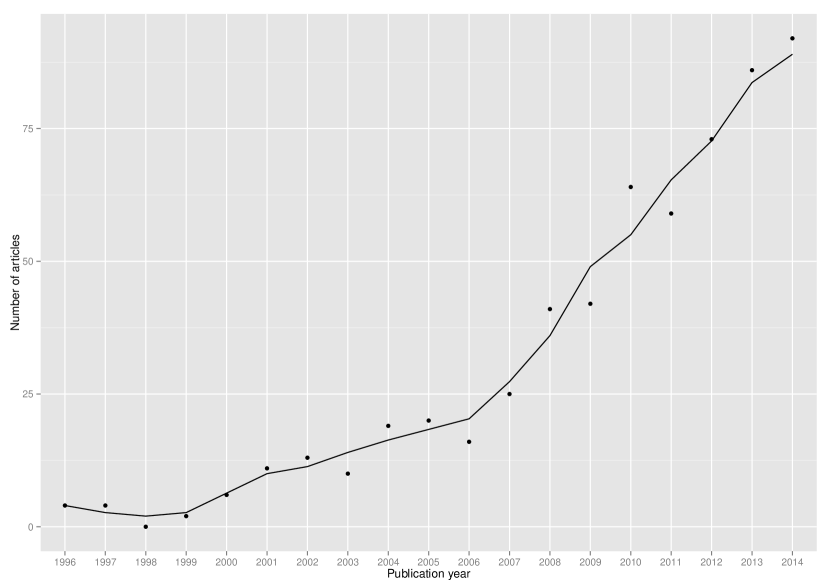
Figure 2: Number of published articles by year of publication and $3$-year moving average

One can interpret the growth shown in figure 2 in three stages. First, in the $1996-2000$ time period, there were a relatively small number of publications, not due to the lack of theoretical results, but rather for the absence of a systematic exposition to BMA and accessible computational tools. Then, with the publication of the revisions by Hoeting et al. (1999), Wasserman (2000) and Geweke (1999) and some computational tools implementing the results by Raftery (1996), Volinsky et al. (1997), Madigan and Raftery (1994) and Madigan et al. (1995) led to a popularization of BMA resulting in a growth in publications in the $2000-2005$ time period. Then, after $2005$, there was a veritable increase in the number of publications, probably due to the widespread use of the aforementioned computational tools, more easily accessible computer power and the increasing availability of ready-to-use MCMC software.

We then divided the database according to the journal title, to identify fields with a more widespread application of BMA. There was no single periodical responsible for most of the literature and it is clear that its applications have spread through diverse fields. The $100$ titles with the higher counts of publications are listed in Table LABEL:T:Periodicals.

There are some clusters representing some patterns in the diffusion and application of BMA. As it is expected from a statistical methodology, there were many articles published in Statistics and Machine Learning periodicals, adding up to $21$ periodicals in the top $100$. There is also a widespread application of BMA in the Economics literature, with $21$ titles in the top $100$ and a few periodicals in Meteorology and Climatology, following the seminal predictive framework proposed by Raftery et al. (2005).

Table 2: Number of publications on the $100$ periodicals with most BMA articles

Title	Articles published	Percentage
Weather Resources Research	18	3.07
Monthly Weather Research	15	2.56
Journal of the American Statistical Association	12	2.04
Journal of Applied Economics	11	1.87
Computational Statistics and Data Analysis	10	1.7
Journal of Hydrology	10	1.7
Biometrics	9	1.53
Economic Modeling	8	1.36
Canadian Journal of Fisheries and Aquatic Sciences	7	1.19
Journal of Econometrics	7	1.19
Statistics in Medicine	7	1.19
Biometrika	6	1.02
Journal of Applied Statistics	6	1.02
Ecological Economics	6	1.02
Journal of Forecasting	6	1.02
Journal of Hydrologic Engineering	6	1.02
Neuroimage	6	1.02
Public Library of Science - One (PLOS-ONE)	6	1.02
Advances in Water Research	5	0.85
International Journal of Forecasting	5	0.85
Journal of Agricultural Biological and Environmental Statistics	5	0.85
Journal of International Money and Finance	5	0.85
Journal of Macroeconomics	5	0.85
Risk Analysis	5	0.85
Stochastic Environmental Research and Risk Analysis	5	0.85
Annals of Applied Statistics	4	0.68
Applied Economics	4	0.68
Bioinformatics	4	0.68
Ecological Applications	4	0.68
Environmental Modeling and Software	4	0.68
Genetic Epidemiology	4	0.68
Hydrology and Earth System Sciences	4	0.68
Journal of Computational and Graphical Statistics	4	0.68
Journal of Machine Learning and Research	4	0.68
Journal of the Royal Statistical Society-B	4	0.68
Technometrics	4	0.68
Applied Economics Letters	3	0.51
BMC-Bioinformatics	3	0.51
Conservation Biology	3	0.51
Cerebral Cortex	3	0.51
Climate Dynamics	3	0.51
Economic Journal	3	0.51
Global and Planetary Change	3	0.51
Journal of Applied Metereology and Climatology	3	0.51
Journal of Business and Economic Statistics	3	0.51
Journal of Banking and Finance	3	0.51
Journal of Gerontology-A	3	0.51
Journal of Geophysical Research: Atmospheres	3	0.51
Machine Learning	3	0.51
Quarterly Journal of the Royal Metereological Society	3	0.51
The Review of Economics and Statistics	3	0.51
Statistics and Computing	3	0.51
Statistical Science	3	0.51
Tellus-A	3	0.51
Annals of Human Genetics	2	0.34
Asia and Pacific Journal of Atmospheric Sciences	2	0.34
Applied Stochastic Models in Business and Industry	2	0.34
Bayesian Analysis	2	0.34
BMC-Systems Biology	2	0.34
Biostatistics	2	0.34
Canadian Journal of Fisheries	2	0.34
Clinical Trials	2	0.34
Economics Bulletin	2	0.34
Environmetrics	2	0.34
Environmental Monitoring and Assessment	2	0.34
Econometric Reviews	2	0.34
Economic Systems	2	0.34
Ensayos sobre politica economica	2	0.34
Freshwater Biology	2	0.34
Forest Ecology and Management	2	0.34
Fisheries Research	2	0.34
Geophysical Research Letters	2	0.34
Genetics Selection Evolution	2	0.34
Human Heredity	2	0.34
Hydrological Processes	2	0.34
Institute of Electrical and Electronics Engineers-B	2	0.34
Institute of Electrical Engineers Transactions	2	0.34
International Journal of Distributed Sensor Networks	2	0.34
International Journal of Environmental Research and Public Health	2	0.34
Journal of Animal Science	2	0.34
Journal of Biogeography	2	0.34
Journal of Computational Physics	2	0.34
Journal of Environmental Economics and Management	2	0.34
Journal of Economic Growth	2	0.34
Journal of Economic Surveys	2	0.34
Journal of the Japanese Statistical Society	2	0.34
Journal of Money, Credit and Banking	2	0.34
Journal of the Royal Statistical Society-A	2	0.34
Journal of the Royal Statistical Society-C	2	0.34
Journal of the Royal Statistical Society-D	2	0.34
Marine Mammal Science	2	0.34
Monthly Notices of the Royal Astronomical Society	2	0.34
Political Analysis	2	0.34
Public Library of Science- Computational Biology	2	0.34
Physical Review D	2	0.34
The Review of Financial Studies	2	0.34
Regional Studies	2	0.34
Systematic Biology	2	0.34
Others	210	35.78
Total	587	100

We also classified each article with respect to the authors and co-authors and listed the top $10$ most productive authors in Table 3 to infer the most massive contributions to the literature. There were no authors overwhelmingly present in the literature given its size, but one can single out the contributions of Adrian Raftery from the University of Washington. Raftery authored or co-authored $34$ articles in our dataset, more than three times the second most productive author and contributed to the theoretical underpinnings of BMA (Kass and Raftery, 1995; Raftery, 1996) and to its applications, for instance in genetics (Yeung et al., 2005), engineering (Raftery et al., 2010), economics (Eicher et al., 2011) and proposed an ensemble prediction method in meteorology and climatology (Raftery et al., 2005) that enjoys widespread use.

Table 3: Top $10$ authors in the BMA literature in number of publications

Name	Institution	Number of authored/co-authored articles
Adrian E. Raftery	University of Washington	34
Tilmann Gneiting	Karlsruhe Institute of Technology	11
Merlyse Clyde	Duke University	10
Q. J. Wang	CSIRO Land and Water	9
Theo S. Eicher	University of Washington	8
Gary Koop	University of Strathclyde	8
David Madigan	Columbia University	7
Xuesong Zhang	Pacific Northwest National Laboratory	7
Edward L. Boone	Virginia Commonwealth University	6
Jesus Crespo-Cuaresma	Vienna University of Economics and Business	6

Following, there are Tilmann Gneiting who mainly contributed to ensemble methods in Meteorology, Merlyse Clyde, who applied BMA mostly in the context of variable selection for regression models using Stochastic Search Variable Selection, Q. J. Wang with contributions in Metereology, Theo S. Eicher and Gary Koop , who applied BMA to Economics, David Madigan, who was part of the seminal BMA works in the late $1990s$, Xuesong Zhang with contributions in Hydrology, Edward L. Boone who used BMA in Ecology and Jesus Crespo-Cuaresma in Economics.

4.2 Conceptual classification scheme

We present below some brief descriptive statistics and discussion on the classification patterns generated using the Conceptual Classification Scheme (CCS) to the dataset, with some notes to trends and guidance to specific applications of BMA. It is not useful to list the hundreds of revised articles, so we aim to provide illustrative works for each aspect of our revision as a the interested reader can follow through its references and citations for his own purposes. Furthermore, the dataset of all responses to the CCS can be obtained upon request from the corresponding author and full citations of the revised articles can be found as a Supplement to this article.

4.2.1 Usage

The most common usage of BMA in the revised literature was model choice, with $231$ works totaling almost $40\%$ of all articles and the overwhelming majority of the revised articles deal with model choice through variable selection in regression models. Overall, we could spot three overarching themes in model choice throughout the literature with eventual variations.

Firstly, there is the application of the background introduced by Adrian Raftery and collaborators in the first half of the $1990s$. These works perform dimensionality reduction of the model space through Occam’s Window or Leaps and Bounds and approximate the model evidence using BIC like Volinsky et al. (1997), in which variable selection and model averaging is performed for a Cox regression model. This set of techniques enjoy great popularity to this date due in part to its implementation in the BMA R package (Raftery and Painter, 2005).Secondly, there are many works concerned with model selection in the linear model, specially in economical applications. Either all $2^{p}$ possible models are considered or there is a stochastic search using MC3 and model evidences are derived explicitly from a conjugate priors (Fernandez et al., 2001b). Finally, there is model choice using stochastic search through MCMC methods, like Reversible Jump MCMC over spaces with different numbers of covariates (Lunn, 2008) and Stochastic Search Variable Selection (Brown et al., 2002).

After model choice, the most popular usage was the combination of multiple models for prediction, which was performed in $161$ articles (around $28\%$ of the dataset). While combining each model’s prediction is straightforward in principle, we identified at least three different trends.

First, there is the straightforward application of BMA by fitting all models to the data, calculating model evidences, generating a prediction from each model’s predictive distribution culminating in a combined prediction. This practice leads to lower risk predictions under a logarithmic loss (Madigan and Raftery, 1994) and is relatively widespread in the literature, with applications in Ecology (Wintle et al., 2003) and Genetics (Annest et al., 2009). Secondly, there is a compromise between variable selection and prediction through an application of BMA to select the models or covariates with highest posterior model probability and the selected model is then used to derive predictions. This procedure employs the machinery developed for variable selection in favor of prediction, like SSVS (Lamon and Clyde, 2000) or RJMCMC (Jacobson and Karlsson, 2004). Finally, there is an alternative use of BMA ideas proposed in Raftery et al. (2005) for meteorological applications that differs somewhat of usual applications and that we will briefly discuss below.

The authors consider the problem of combining forecasts from $K$ models, $f_{1},\ldots,f_{K}$ into one combined prediction. For each forecast there is a probability density function for the quantity one wished to forecast $y$ denoted by $g_{l}(y|f_{l})$ for $l=1,\ldots,K$. Raftery et al. (2005) then proposes to construct a combined density function using the weighted average

$$g(y|f_{1},\ldots,f_{K})=\sum_{l=1}^{K}w_{l}g_{l}(y|f_{l}),$$ (17)

in which $\sum_{l=1}^{K}w_{l}=1$, and the weights are interpreted in an analogous fashion to the posterior model probabilities in usual BMA. Assuming then each density as a normal, the authors estimate the weights using the EM Algorithm. This method has spread widely on the specialized literature, and albeit no strong theoretical optimality seems to exist, it enjoys adequate performance in Meteorological and Climatological applications.

Bayesian model averaging is used for combined estimation in $111$ articles (around $19\%$) throughout our revision. Albeit similar in purpose with combined prediction, we classified a work as a combined estimation article if its purpose was to estimate a common parameter to all models, but not a future observation. Combined estimators were employed to estimate a variety of quantities that might be appropriately modeled by plenty of models, such as population size (King and Brooks, 2001), toxicity in clinical trials (Yin and Yuan, 2009), breeding values in genetics (Habier et al., 2010) and the probability of an economic recession (Guarín et al., 2014).

Conceptual discussions and methodological articles ammounted for $65$ data points (around $11\%$ of the dataset). This category presents a clear heterogeneity, as it comprises theoretical and conceptual advances in many directions. Articles in this category are, however, very similar with respect to its purpose to introduce an application of BMA to an existing problem or extend BMA to overcome limitations in some settings.

The former articles refer to seminal theoretical works like Raftery (1996), that introduced the BIC approximation to the Bayes factor and paved the way for many subsequent works. There were also pioneer works discussing the introduction of BMA to applied fields, like the methodology discussed in Fernandez et al. (2001a) for variable selection in economical applications. Its use of Zellner’s $g-$prior (Zellner, 1986) for the regression coefficients (allowing for explicit model evidences) and MC3 composition for model space search were quickly adopted by many authors in very diverse economical studies. The introduction of BMA to the problem of selecting network structures in Bayesian Networks (Friedman and Koller, 2003) also had a great impact in the Machine Learning literature, spawning a wealth of approximations for the ideal Bayesian averaged network. Finally, there were also novel developments in BMA that made it usable within a field. For instance, the variational Bayes approximation for the evidence proposed in Friston et al. (2007) sparked plenty of BMA applications to neurological datasets. On the other hand, the latter articles deal with extensions of BMA to different Bayesian applications, like the BMA under sequential updating discussed in Raftery et al. (2010).

The last category we employed to classify articles on usage pertains to review articles on BMA or the applications of model averaging to specific fields or models. There are $18$ such articles in our dataset, amounting to less than $3\%$ of the total. Some of the revision articles sparked the application of BMA in general like the seminal works by Hoeting et al. (1999) and Wasserman (2000), whereas more specific revisions exposed the methodology in other fields like Economics (Geweke, 1999), Genetics (Fridley, 2009) and Physics (Parkinson and Liddle, 2013). There are also revisions on model selection (Kadane and Lazar, 2004) and model uncertainty (Clyde and George, 2004) in which BMA figures as a technique.

4.2.2 Field of application

As stated in Section 3.2, we classified the dataset into four main categories to give a broad idea of the application of BMA in different fields. We divided our dataset into four categories regarding applications in the Biological and Life Sciences, Humanities and Economics, Physical Sciences and Engineering and Statistics and Machine Learning, respectively in order to infer if there was an increased penetration of BMA in either field.

Figure 3: Usage of BMA by field of application

The field with most articles was Life Sciences and Medicine, with $201$ works corresponding to $34.24\%$ of all reviewed publications. Within these publications, there are some trends of note. In the medical sciences, BMA was used mostly for model choice purposes, as in variable selection of factors associated with false positives in diagnostic kits (Ranyimbo and Held, 2006), weight loss (Phelan et al., 2009), leukemia progression (Oehler et al., 2009), structure in Bayesian networks for patient-specific models (Visweswaran et al., 2010) and the combined estimation as in Yin and Yuan (2009). BMA was also used extensively in Ecology, with applications to landscape ecology and geographical information systems (Barber et al., 2006), prediction of species distribution (Thomson et al., 2007), capture-recapture models (Arnold et al., 2010) and evolution (Silvestro et al., 2014).

The massive number of genetic variables obtained from biomarkers like microarrays and Single Nucleotide Polymorphisms (SNPs) that relate with observed characteristics through complex interactions fostered a rich Bayesian model selection literature in Genetics. BMA was employed to combine and select genetic information from metabolic pathways (Conti et al., 2003), quantitative trait loci (Boone et al., 2008), candidate SNPs for lung cancer risk (Swartz et al., 2013) and a revision of Bayesian model selection models was performed in Fridley (2009). There is also the seminal work by Meuwissen and Goddard (2001) that introduced a class of SSVS-like estimation procedure in quantitative genetics that gained much traction in the Animal and Plant sciences literature, concerned with the prediction of genetic merit for selection (Kizilkaya et al., 2010; Boddhireddy et al., 2014). There also seems to be an increase of model averaging in neuroscience using the methods introduced by Penny et al. (2010).

The Humanities and Economy field had $149$ articles ($25.38\%$ of the dataset), with the overwhelming majority being in economical applications. The earliest application to economics in our dataset is the revision of Bayesian modeling by Geweke (1999). The most adopted framework for model selection using BMA was introduced in Fernandez et al. (2001a), describing conjugate priors and a model search procedure that enjoys a broad application to many economical questions to this date, although were also articles applying the framework introduced by Adrian Raftery and collaborators through the R package this group developed like done in Goenner (2010) and applications of SSVS (Vrontos et al., 2008). Forecasting using BMA in economical settings was discussed in Koop and Potter (2004) and was adopted by many subsequent articles. There were also some occasional applications to Political Science mostly on variable selection as in trade interdependence in conflict (Goenner, 2004) and some forecasting, like the study of the $2000$ american presidential election in Sidman et al. (2008).

The application of BMA in the Physical Sciences and Engineering amounted for $146$ articles, about $24.82\%$ of the total. Most of this field was made of applications to forecasting problems in Meteorology and Climatology stemming from the seminal work of Raftery et al. (2005) in the field, using the ideas of BMA into an ensemble forecast with posterior model probabilities estimated using the EM algorithm. There were also some works in Physics, like the study of dark matter in Liddle et al. (2006) and the revision of BMA methods in astrophysics in Parkinson and Liddle (2013).

Finally, there were $92$ articles in the Statistics and Machine Learning field. There are some methodological articles, like Raftery (1996) on the BIC approximation and revisions on BMA like the highly influential Hoeting et al. (1999) and Wasserman (2000) and model uncertainty (Kadane and Lazar, 2004; Clyde and George, 2004). There were also some developments in model choice to more statistically sophisticated models like Generalized Linear Models (GLMs, Morales et al. (2006)), transformations (Hoeting et al., 2002) and Generalized Auto-Regressive Conditional Heteroskedasticity (GARCH) models (Chen et al., 2011). In the Machine Learning literature, BMA was mostly used along with Bayesian Networks (Friedman and Koller, 2003), with theoretical developments allowing for the direct estimation of the averaged network without the necessity of the usual estimation procedure of estimating and combining all posteriors (Dash and Cooper, 2004; Cerquides and De Mántaras, 2005).

Since our revision spans through very diverse fields with very different questions, we investigated how these research questions were reflected in usage throughout the fields. A graphical summary can be observed in Figure 3. Combined prediction is more common in the Physical Sciences field, which is mostly explained by the abundance of prediction articles using the ensemble method by Raftery et al. (2005). Economics research questions seemed to focus more on the search for influent factors and determinants, leading to model and variable selection. Since economics dominated the Humanities and Economics field, one can observe a large number of model choice papers. Model selection was also very present in the Life Sciences and Medicine field, with more than half the revised articles. There is, however, an interest in combined estimation that is larger than other fields. Finally, most of the Statistics and Machine Learning literature revised concerns methodological advancements and discussions.

4.2.3 Model priors

Prior elicitation is a current and open research subject in Bayesian inference as a whole, with distinct currents advocating completely subjectivist researcher-driven prior distributions to completely agnostic and data-driven priors and many types of compromise in between. As discussed in Section 1.1, this problem is compounded in BMA settings, as the space of the conceivable models is a more abstract parametric space, thus harder to measure in terms of a probability measure.

The most common answer to this uncertainty is to assume an uniform distribution over the model space through a vague prior. Such practice is, by far the most common and is adopted by more than $50\%$ of the revised articles, in $297$ publications. Given a finite number of $K$ models, the authors simply assume $\pi(M_{l})=\frac{1}{K}$ for $l=1,\ldots,K$ or an equivalent formulation like assuming a Bernoulli prior with prior inclusions equal to $\frac{1}{2}$ in SSVS. In the case of an infinite number of models like in mixture problems, some authors adopt the alternative proposed in Richardson and Green (1997) of fixing a maximum number of classes and assuming an uniform distribution over the restricted model space.

Some authors circumvent the problem by adopting more traditional prior distributions verbatim from the literature. This practice was present in $98$ articles, around $16.6\%$ of all publications and there seems to be a few trends. Some of this adoption is caused by convenient conceptual frameworks - many authors in the economics literature simply adopted the prior, evidence estimation and model search proposed by Fernandez et al. (2001a) verbatim. With the diffusion of BMA software first by personal request to Adrian Raftery’s group with the S-Plus codes could be obtained by sending an email titled “send BMA from S” to the authors and then by the use of the bma R package, less attention was paid to the priors as many authors simply used whatever was default in these implementations.

We also observed $63$ articles that tackled the problem and derived model priors for posterior BMA. Some noteworthy examples in the literature include Medvedovic and Sivaganesan (2002) that elicited model priors by the expected behavior of the cell cultures under study, the analytical considerations of the Bayesian networks of interest in Friedman and Koller (2003), the combination of multiple stakeholders in Mäntyniemi et al. (2013) and the proposal of a cross-model correlations to elicit model priors in Garthwaite and Mubwandarikwa (2010).

The remainder $130$ articles amount to those that did not specify or apply any model priors. Albeit odd by Bayesian standards, these articles still apply BMA, but priors are not specified. The most common reason in our dataset is of the applications of the ensemble forecast method introduced in Raftery et al. (2005), that just estimates a “posterior” weight using the EM algorithm with no mention of priors. There is also the adoption of default options in software packages for BMA for which we tracked down the default settings when possible, but that was not always possible.

4.2.4 Evidence estimation

The estimation of the marginal likelihood leading to the posterior model probability presents a considerable difficulty to be overcome in the applications of model averaging. As datasets get more complex, thus requiring more complex models, we aimed to investigate how the BMA literature deals with the problem of estimating the model evidence.

The integral in equation (2) is not available in closed form for most likelihoods besides in the (generalized) linear regression model with conjugate priors. These models are however, very popular and its widespread adoption explains most of the $232$ articles we classified as “not applicable” (NA) in our CCS.

With respect to approximations, most revised articles approximated the evidence by analytical means, as done in $190$ articles. Although inferior to the Laplace approximation in theory (Kass and Raftery, 1995; Raftery, 1996) and simulations (Boone et al., 2005), most articles use the BIC approximation, as its value is given by most software available for parameter estimation in generalized linear models, making for a straightforward application of BMA. Its immediate availability from the maximum likelihood estimates, combined with some theory and available software for a wide class of GLMs justify its popularity. Its popularity also makes it the most widely misused approximation. We encountered “approximations” based on other information criteria as a way to improve over the BIC, frequently using the Akaike Information Criteria (AIC), the Deviance Information Criteria (DIC) and other more ad hoc information criteria.

Markov Chain Monte Carlo methods were used to estimate the evidence in $113$ articles. The vast majority of there works use RJMCMC or SSVS methods, and as such, the posterior model probabilities are estimated by the sample average of an indicator variable for each model. There were, however, plenty of articles that employed the Importance Sampling approach by Gelfand and Dey (1994) and the much criticized harmonic mean estimator (Newton and Raftery, 1994), as they are simpler to implement in complex models than the trans-dimensional proposals and transformation required for RJMCMC. Still in spirit with MCMC but using a different technique, $17$ articles used the ratio of densities (Chib, 1995) approach.

We also encountered $36$ articles in which the evidence was estimated through the use of Monte Carlo integration techniques (using independent samples, in constrast with the dependent Markov Chain samples used in MCMC), but there was no unifying trend over the practice. Most authors used importance methods, like Sampling-Importance-Resampling (SIR), in which a size $n$ sample is taken from the prior distributions and used to construct importance weights using the likelihood. Posterior samples are them obtained from resampling $m<n$ values with replacement using the constructed weights. With these samples, posterior inference and evidence estimation are direct even for complex models, like the stochastic differential equation model used in Bunnin et al. (2002).

4.2.5 Dimensionality

As datasets get more massive and models more complex to aggregate different sources of information, it is common that large model spaces emerge. For instance, in the Genomics literature, the development of high throughput marker chips generated millions of Single Nucleotide Polymorphism (SNP) variables one desires to associate with a response variable inducing a dimensionality problem. As mentioned in Section 3.5, we investigated two approaches: previous filtering and stochastic search through Markov Chains.

Between these two approaches, stochastic search was the most prevalent one, with $144$ articles. Among these papers, there are three main trends. With the abundance of BMA in regression models, plenty of the literature was concerned with variable selection, which led to the widespread application of dedicated methods like SSVS that allow for a direct measure of association strength through the marginal posterior inclusion probabilities. A typical example of SSVS can be encountered in Blattenberger et al. (2012) applied to the search for risk factors related to the use of cell phones while driving. The Markov Chain Monte Carlo Model Composition (MC3, Madigan et al. (1995)) was also widely applied in variable selection settings, mainly in the economics literature following the seminal work by Fernandez et al. (2001b). MC3 in turn is very similar in spirit with the Reversible Jump MCMC methods, which were mostly employed in our revision to choose between complex models instead of variable selection, like done in Wu and Drummond (2011).

Some authors chose to perform a prior dimensionality reduction in the model space and then apply the model averaging, as done in $103$ articles in our dataset, most of them on variable selection for regression models. Among these prior reductions, the most popular was the Occam’s Window criterion (Madigan and Raftery, 1994), probably due to its implementation in the bma R package. In some works, some applied the Leaps and Bounds algorithm (Furnival and Wilson, 1974) prior to the Occam’s Window to select highly likely variable subsets without the need of an exhaustive calculation.

However, there were cases where authors performed exhaustive calculations for all possible models and many cases where the number of models under consideration were small, leading to the $341$ articles marked as “not applicable” (NA) in our dataset.

4.2.6 Markov Chain Monte Carlo methods

We investigated the application of MCMC methods throughout our dataset. For this particular classification, we excluded $24$ works that either presented purely revisions or conceptual discussions and did not apply any estimation methodology and articles in which BMA was applied but poorly described to the point we could not tell whether MCMC methods were used anywhere. The remainder $563$ articles were classified to their usage of MCMC or lack thereof. In our dataset, $261$ articled applied MCMC methods, whereas $302$ did not.

The temporal pattern of MCMC usage, separated by publication year can be found in Figure 4. Although we suspected that MCMC would become more popular after the popularization of freely available software, it seems like MCMC methods were not as prevalent in the literature as expected and its usage did not increase much even with more available software and cheaper computational power. MCMC was applied in approximately half the articles published in any given year with the exception of the early years of the $2000$s.

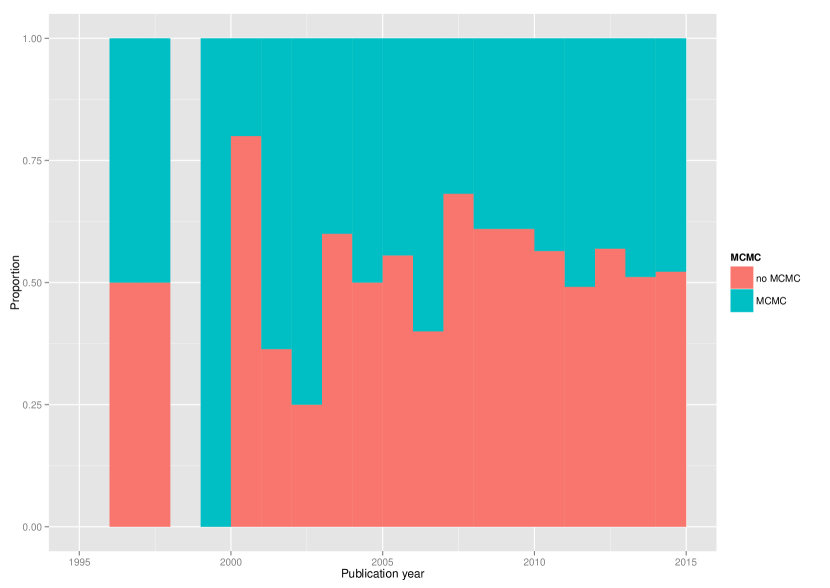
Figure 4: Markov Chain Monte Carlo methods usage in the dataset

4.2.7 Simulation studies

Our dataset was also classified with respect to the presence of simulation studies. Overall, $19$ articles were not clear on their usage of simulations, and were therefore excluded from this classification. Of the remaining articles, the majority composed of $375$ articles did not perform any form of simulations, whereas $193$ did some sort of simulation study.

A more detailed classification by year of publication can be encountered in Figure 5. As in the MCMC classification, the increased computational power did not seem to have an effect on the realization of simulation studies. One can also observe that simulations seem to be unpopular overall, never accounting for more than half the published papers in any given year.

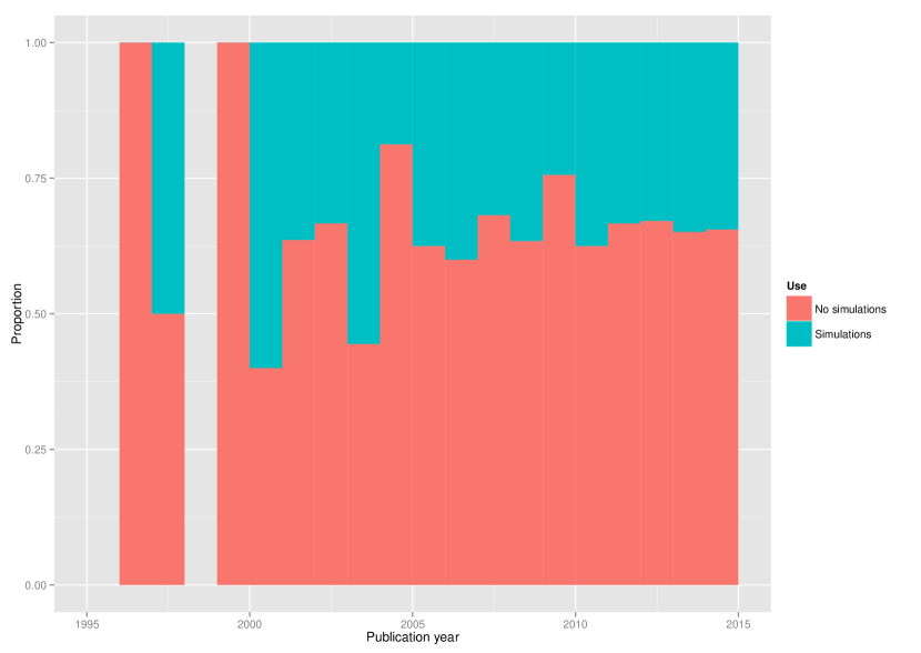
Figure 5: Proportion of simulation studies

4.2.8 Data-driven validation

We classified the literature on the use of data-driven validation of the results obtained by model averaging. The majority of articles ($358$ papers) did not perform any validation whatsoever. Among the articles that performed some kind of data-based validation, the overwhelming majority of $179$ articles used cross-validation by splitting the dataset into two disjoint subsets, fitting the desired models to one of the subsets and validating their performance on the other. The slightly more sophisticated K-fold cross-validation was only applied in $17$ articles.

Curiously, even though BMA is a Bayesian technique, there was only a single application of posterior predictive checks (Barber et al., 2006), a data-driven Bayesian goodness-of-fit criteria based on the posterior distribution deriving conclusions rooted in the Bayesian paradigm.

5 Concluding remarks

This work performed a methodical literature review of Bayesian Model Averaging studies in the $1996-2014$ time period. After a thorough search, we employed a conventional content analysis, and proposed a novel conceptual classification scheme that we applied to the literature, revising and classifying $587$ articles from a large variety of publications spanning a wide range of applications.

Although much was discussed in the formulation of the proposed classification scheme and its results when applied to the selected literature, some limitations to the present work still exist. First, our search was limited to peer-reviewed articles published in digitally available periodicals. As such, many developments in BMA possibly published in conference proceedings, dissertations or theses and books might have been overlooked. Secondly, said periodicals were restricted to the titles listed on the four databases mentioned in Section 2.1 and, albeit an effort was made to be as inclusive with the literature as possible, non-listed titles were not included except when cited in selected articles and passed the exclusion criteria. Finally, the search was initiated through specific queries on these databases, and as such, relevant articles might have been overlooked when we restricted terms.

Limitations aside, this revision can provide relevant insights into the current BMA literature and some indications of future developments. With no aspiration to be exhaustive, we point out a few. Namely, we have five observations:

1. The methodology provides for a very flexible account of model uncertainty which can in principle be applied to any problem, but not much was done in model choice using BMA aside from variable selection in regression models, with the exception of BMA in Bayesian Networks present in the Machine Learning literature of the early $2000$s.

2. Not much was done in methodological developments in the statistical literature aside from the seminal works in the late $1990$s, limiting its application mostly to (generalized) linear regression models in spite of more complex models being proposed in the same time period. For instance, the problem of evidence estimation is still either circumvented by using convenient likelihoods and conjugate priors or solved through the BIC approximation, which, being reliant on plenty of regularity conditions, might not be adequate for more complex models. Much of the developments in MCMC after the textbook algorithms (i.e. straightforward applications of the Gibbs’s Sampler and Metropolis-Hastings algorithms) were also mostly absent from our dataset.

3. There was no significant discussion on computational costs of BMA. There are distinct computational problems derived from dealing with very large datasets, very large and complex model spaces and in the fit of complex models that were not approached in the revised literature.

4. The vague prior is still the most used model prior and, albeit convenient it might not be the best choice for all problems. Not much was done in prior elicitation or the reference priors for BMA.

5. Neither simulation studies or validation methods were popular in the literature. This presents a very serious issue, as BMA usually deals with many models drawing from sometimes very distinct assumptions and therefore reaching distinct conclusions. Using BMA without any validation might lead to an overconfidence in the conclusions, the very problem model averaging is proposed to mitigate.

References

- (1)
- Annest et al. (2009) Annest, A., Bumgarner, R. E., Raftery, A. E. and Yeung, K. Y. (2009). Iterative bayesian model averaging: a method for the application of survival analysis to high-dimensional microarray data, BMC bioinformatics 10(1): 72.
- Arnold et al. (2010) Arnold, R., Hayakawa, Y. and Yip, P. (2010). Capture–recapture estimation using finite mixtures of arbitrary dimension, Biometrics 66(2): 644–655.
- Barber et al. (2006) Barber, J. J., Gelfand, A. E. and Silander, J. A. (2006). Modelling map positional error to infer true feature location, Canadian Journal of Statistics 34(4): 659–676.
- Blattenberger et al. (2012) Blattenberger, G., Fowles, R., Loeb, P. D. and Clarke, W. A. (2012). Understanding the cell phone effect on vehicle fatalities: a bayesian view, Applied Economics 44(14): 1823–1835.
- Boddhireddy et al. (2014) Boddhireddy, P., Kelly, M., Northcutt, S., Prayaga, K., Rumph, J. and DeNise, S. (2014). Genomic predictions in angus cattle: comparisons of sample size, response variables, and clustering methods for cross-validation, Journal of animal science 92(2): 485–497.
- Boone et al. (2008) Boone, E. L., Simmons, S. J., Bao, H. and Stapleton, A. E. (2008). Bayesian hierarchical regression models for detecting qtls in plant experiments, Journal of Applied Statistics 35(7): 799–808.
- Boone et al. (2005) Boone, E. L., Ye, K. and Smith, E. P. (2005). Assessment of two approximation methods for computing posterior model probabilities, Computational statistics & data analysis 48(2): 221–234.
- Brown et al. (2002) Brown, P. J., Vannucci, M. and Fearn, T. (2002). Bayes model averaging with selection of regressors, Journal of the Royal Statistical Society: Series B (Statistical Methodology) 64(3): 519–536.
- Bunnin et al. (2002) Bunnin, F. O., Guo, Y. and Ren, Y. (2002). Option pricing under model and parameter uncertainty using predictive densities, Statistics and Computing 12(1): 37–44.
- Cerquides and De Mántaras (2005) Cerquides, J. and De Mántaras, R. L. (2005). Tan classifiers based on decomposable distributions, Machine Learning 59(3): 323–354.
- Chen et al. (2011) Chen, C. W., Liu, F. C. and Gerlach, R. (2011). Bayesian subset selection for threshold autoregressive moving-average models, Computational Statistics 26(1): 1–30.
- Chib (1995) Chib, S. (1995). Marginal likelihood from the gibbs output, Journal of the American Statistical Association 90(432): 1313–1321.
- Clyde and George (2004) Clyde, M. and George, E. I. (2004). Model uncertainty, Statistical science pp. 81–94.
- Conti et al. (2003) Conti, D. V., Cortessis, V., Molitor, J. and Thomas, D. C. (2003). Bayesian modeling of complex metabolic pathways, Human heredity 56(1-3): 83–93.
- Dash and Cooper (2004) Dash, D. and Cooper, G. F. (2004). Model averaging for prediction with discrete bayesian networks, The Journal of Machine Learning Research 5: 1177–1203.
- Eicher et al. (2011) Eicher, T. S., Papageorgiou, C. and Raftery, A. E. (2011). Default priors and predictive performance in bayesian model averaging, with application to growth determinants, Journal of Applied Econometrics 26(1): 30–55.
- Fernandez et al. (2001b) Fernandez, C., Ley, E. and Steel, M. F. (2001b). Model uncertainty in cross-country growth regressions, Journal of applied Econometrics 16(5): 563–576.
- Fernandez et al. (2001a) Fernandez, C., Ley, E. and Steel, M. F. J. (2001a). Benchmark priors for bayesian model averaging, Journal of Econometrics 100(2): 381–427.
- Fridley (2009) Fridley, B. L. (2009). Bayesian variable and model selection methods for genetic association studies, Genetic epidemiology 33(1): 27–37.
- Friedman and Koller (2003) Friedman, N. and Koller, D. (2003). Being bayesian about network structure. a bayesian approach to structure discovery in bayesian networks, Machine learning 50(1-2): 95–125.
- Friel and Wyse (2012) Friel, N. and Wyse, J. (2012). Estimating the evidence–a review, Statistica Neerlandica 66(3): 288–308.
- Friston et al. (2007) Friston, K., Mattout, J., Trujillo-Barreto, N., Ashburner, J. and Penny, W. (2007). Variational free energy and the laplace approximation, Neuroimage 34(1): 220–234.
- Furnival and Wilson (1974) Furnival, G. M. and Wilson, R. W. (1974). Regressions by leaps and bounds, Technometrics 16(4): 499–511.
- Garthwaite and Mubwandarikwa (2010) Garthwaite, P. H. and Mubwandarikwa, E. (2010). Selection of weights for weighted model averaging, Australian & New Zealand Journal of Statistics 52(4): 363–382.
- Gelfand and Dey (1994) Gelfand, A. E. and Dey, D. K. (1994). Bayesian model choice: asymptotics and exact calculations, Journal of the Royal Statistical Society. Series B (Methodological) pp. 501–514.
- Gelman and Meng (1998) Gelman, A. and Meng, X. (1998). Simulating normalizing constants: From importance sampling to bridge sampling to path sampling, Statistical science pp. 163–185.
- Gelman et al. (1996) Gelman, A., Meng, X. and Stern, H. (1996). Posterior predictive assessment of model fitness via realized discrepancies, Statistica sinica 6(4): 733–760.
- George and McCulloch (1993) George, E. I. and McCulloch, R. E. (1993). Variable selection via gibbs sampling, Journal of the American Statistical Association 88(423): 881–889.
- George and McCulloch (1997) George, E. I. and McCulloch, R. E. (1997). Approaches for bayesian variable selection, Statistica sinica 7(2): 339–373.
- Geweke (1999) Geweke, J. (1999). Using simulation methods for bayesian econometric models: inference, development, and communication, Econometric Reviews 18(1): 1–73.
- Goenner (2004) Goenner, C. F. (2004). Uncertainty of the liberal peace, Journal of Peace Research 41(5): 589–605.
- Goenner (2010) Goenner, C. F. (2010). Discrimination and mortgage lending in boston: The effects of model uncertainty, The Journal of Real Estate Finance and Economics 40(3): 260–285.
- Green (1995) Green, P. J. (1995). Reversible jump markov chain monte carlo computation and bayesian model determination, Biometrika 82(4): 711–732.
- Guan and Stephens (2011) Guan, Y. and Stephens, M. (2011). Bayesian variable selection regression for genome-wide association studies and other large-scale problems, The Annals of Applied Statistics pp. 1780–1815.
- Guarín et al. (2014) Guarín, A., González, A., Skandalis, D. and Sánchez, D. (2014). An early warning model for predicting credit booms using macroeconomic aggregates, Ensayos Sobre Política Económica 32(SPE73): 77–86.
- Habier et al. (2010) Habier, D., Tetens, J., Seefried, F., Lichtner, P. and Thaller, G. (2010). The impact of genetic relationship information on genomic breeding values in german holstein cattle, Genetics Selection Evolution 42(1): 5.
- Hachicha and Ghorbel (2012) Hachicha, W. and Ghorbel, A. (2012). A survey of control-chart pattern-recognition literature (1991–2010) based on a new conceptual classification scheme, Computers & Industrial Engineering 63(1): 204–222.
- Hoeting et al. (1999) Hoeting, J. A., Madigan, D., Raftery, A. E. and Volinsky, C. T. (1999). Bayesian model averaging: a tutorial, Statistical science pp. 382–401.
- Hoeting et al. (2002) Hoeting, J. A., Raftery, A. E. and Madigan, D. (2002). Bayesian variable and transformation selection in linear regression, Journal of Computational and Graphical Statistics 11(3): 485–507.
- Hsieh and Shannon (2005) Hsieh, H.-F. and Shannon, S. E. (2005). Three approaches to qualitative content analysis, Qualitative health research 15(9): 1277–1288.
- Jacobson and Karlsson (2004) Jacobson, T. and Karlsson, S. (2004). Finding good predictors for inflation: A bayesian model averaging approach, Journal of Forecasting 23(7): 479–496.
- Kadane and Lazar (2004) Kadane, J. B. and Lazar, N. A. (2004). Methods and criteria for model selection, Journal of the American statistical Association 99(465): 279–290.
- Kass and Raftery (1995) Kass, R. E. and Raftery, A. E. (1995). Bayes factors, Journal of the american statistical association 90(430): 773–795.
- King and Brooks (2001) King, R. and Brooks, S. (2001). On the bayesian analysis of population size, Biometrika 88(2): 317–336.
- Kizilkaya et al. (2010) Kizilkaya, K., Fernando, R. and Garrick, D. (2010). Genomic prediction of simulated multibreed and purebred performance using observed fifty thousand single nucleotide polymorphism genotypes, Journal of animal science 88(2): 544–551.
- Koop and Potter (2004) Koop, G. and Potter, S. (2004). Forecasting in dynamic factor models using bayesian model averaging, The Econometrics Journal 7(2): 550–565.
- Lamon and Clyde (2000) Lamon, E. C. and Clyde, M. A. (2000). Accounting for model uncertainty in prediction of chlorophyll a in lake okeechobee, Journal of agricultural, biological, and environmental statistics pp. 297–322.
- Leamer (1978) Leamer, E. E. (1978). Specification searches, New York: Wiley.
- Liddle et al. (2006) Liddle, A. R., Mukherjee, P., Parkinson, D. and Wang, Y. (2006). Present and future evidence for evolving dark energy, Physical Review D 74(12): 123506.
- Lunn (2008) Lunn, D. J. (2008). Automated covariate selection and bayesian model averaging in population pk/pd models, Journal of pharmacokinetics and pharmacodynamics 35(1): 85–100.
- Madigan and Raftery (1994) Madigan, D. and Raftery, A. E. (1994). Model selection and accounting for model uncertainty in graphical models using occam’s window, Journal of the American Statistical Association 89(428): 1535–1546.
- Madigan et al. (1995) Madigan, D., York, J. and Allard, D. (1995). Bayesian graphical models for discrete data, International Statistical Review/Revue Internationale de Statistique pp. 215–232.
- Mäntyniemi et al. (2013) Mäntyniemi, S., Haapasaari, P., Kuikka, S., Parmanne, R., Lehtiniemi, M., Kaitaranta, J. and Hilborn, R. (2013). Incorporating stakeholders’ knowledge to stock assessment: Central baltic herring, Canadian Journal of Fisheries and Aquatic Sciences 70(4): 591–599.
- Medvedovic and Sivaganesan (2002) Medvedovic, M. and Sivaganesan, S. (2002). Bayesian infinite mixture model based clustering of gene expression profiles, Bioinformatics 18(9): 1194–1206.
- Meuwissen and Goddard (2001) Meuwissen, T. E. Hayes, B. J. and Goddard, M. E. (2001). Prediction of total genetic value using genome-wide dense marker maps, Genetics 157(4): 1819–1829.
- Moher et al. (2009) Moher, D., Liberati, A., Tetzlaff, J. and Altman, D. G. (2009). Preferred reporting items for systematic reviews and meta-analyses: the prisma statement, Annals of internal medicine 151(4): 264–269.
- Morales et al. (2006) Morales, K. H., Ibrahim, J. G., Chen, C.-J. and Ryan, L. M. (2006). Bayesian model averaging with applications to benchmark dose estimation for arsenic in drinking water, Journal of the American Statistical Association 101(473): 9–17.
- Newton and Raftery (1994) Newton, M. A. and Raftery, A. E. (1994). Approximate bayesian inference with the weighted likelihood bootstrap, Journal of the Royal Statistical Society. Series B (Methodological) pp. 3–48.
- Oehler et al. (2009) Oehler, V. G., Yeung, K., Choi, Y. E., Bumgarner, R. E., Raftery, A. E. and Radich, J. P. (2009). The derivation of diagnostic markers of chronic myeloid leukemia progression from microarray data, Blood 114(15): 3292–3298.
- Parkinson and Liddle (2013) Parkinson, D. and Liddle, A. R. (2013). Bayesian model averaging in astrophysics: a review, Statistical Analysis and Data Mining: The ASA Data Science Journal 6(1): 3–14.
- Penny et al. (2010) Penny, W. D., Stephan, K. E., Daunizeau, J., Rosa, M. J., Friston, K. J., Schofield, T. M. and Leff, A. P. (2010). Comparing families of dynamic causal models, PLoS Comput Biol 6(3): e1000709–e1000709.
- Phelan et al. (2009) Phelan, S., Liu, T., Gorin, A., Lowe, M., Hogan, J., Fava, J. and Wing, R. R. (2009). What distinguishes weight-loss maintainers from the treatment-seeking obese? analysis of environmental, behavioral, and psychosocial variables in diverse populations, Annals of Behavioral Medicine 38(2): 94–104.
- Plummer (2003) Plummer, M. (2003). Jags: A program for analysis of bayesian graphical models using gibbs sampling, Proceedings of the 3rd international workshop on distributed statistical computing, Vol. 124, Technische Universit at Wien, p. 125.
- Raftery (1996) Raftery, A. E. (1996). Approximate bayes factors and accounting for model uncertainty in generalised linear models, Biometrika 83(2): 251–266.
- Raftery et al. (2005) Raftery, A. E., Gneiting, T., Balabdaoui, F. and Polakowski, M. (2005). Using bayesian model averaging to calibrate forecast ensembles, Monthly Weather Review 133(5): 1155–1174.
- Raftery et al. (2010) Raftery, A. E., Kárnỳ, M. and Ettler, P. (2010). Online prediction under model uncertainty via dynamic model averaging: Application to a cold rolling mill, Technometrics 52(1): 52–66.
- Raftery and Painter (2005) Raftery, A. E. and Painter, I. S. (2005). Bma: an r package for bayesian model averaging, R news 5(2): 2–8.
- Ranyimbo and Held (2006) Ranyimbo, A. and Held, L. (2006). Estimation of the false negative fraction of a diagnostic kit through bayesian regression model averaging, Statistics in medicine 25(4): 653–667.
- Richardson and Green (1997) Richardson, S. and Green, P. J. (1997). On bayesian analysis of mixtures with an unknown number of components, Journal of the Royal Statistical Society. Series B (Methodological) pp. 731–792.
- Robert and Casella (2013) Robert, C. and Casella, G. (2013). Monte Carlo statistical methods, Springer Science & Business Media.
- Roberts (1965) Roberts, H. V. (1965). Probabilistic prediction, Journal of the American Statistical Association 60(309): 50–62.
- Sidman et al. (2008) Sidman, A. H., Mak, M. and Lebo, M. J. (2008). Forecasting non-incumbent presidential elections: Lessons learned from the 2000 election, International Journal of Forecasting 24(2): 237–258.
- Silvestro et al. (2014) Silvestro, D., Zizka, G. and Schulte, K. (2014). Disentangling the effects of key innovations on the diversification of bromelioideae (bromeliaceae), Evolution 68(1): 163–175.
- Spiegelhalter et al. (1995) Spiegelhalter, D. J., Thomas, A., Best, N. G. and Gilks, W. R. (1995). Bugs: Bayesian inference using gibbs sampling, version 0.50, MRC Biostatistics Unit, Cambridge .
- Swartz et al. (2013) Swartz, M. D., Peterson, C. B., Lupo, P. J., Wu, X., Forman, M. R., Spitz, M. R., Hernandez, L. M., Vannucci, M. and Shete, S. (2013). Investigating multiple candidate genes and nutrients in the folate metabolism pathway to detect genetic and nutritional risk factors for lung cancer, Plos one 8(1): 1–9.
- Thomson et al. (2007) Thomson, J. R., Mac Nally, R., Fleishman, E. and Horrocks, G. (2007). Predicting bird species distributions in reconstructed landscapes, Conservation Biology 21(3): 752–766.
- Visweswaran et al. (2010) Visweswaran, S., Angus, D. C., Hsieh, M., Weissfeld, L., Yealy, D. and Cooper, G. F. (2010). Learning patient-specific predictive models from clinical data, Journal of biomedical informatics 43(5): 669–685.
- Volinsky et al. (1997) Volinsky, C. T., Madigan, D., Raftery, A. E. and Kronmal, R. A. (1997). Bayesian model averaging in proportional hazard models: assessing the risk of a stroke, Journal of the Royal Statistical Society: Series C (Applied Statistics) 46(4): 433–448.
- Vrontos et al. (2008) Vrontos, S. D., Vrontos, I. D. and Giamouridis, D. (2008). Hedge fund pricing and model uncertainty, Journal of Banking & Finance 32(5): 741–753.
- Wasserman (2000) Wasserman, L. (2000). Bayesian model selection and model averaging, Journal of mathematical psychology 44(1): 92–107.
- Wintle et al. (2003) Wintle, B. A., McCarthy, M. A., Volinsky, C. T. and Kavanagh, R. P. (2003). The use of bayesian model averaging to better represent uncertainty in ecological models, Conservation Biology 17(6): 1579–1590.
- Wu and Drummond (2011) Wu, C.-H. and Drummond, A. J. (2011). Joint inference of microsatellite mutation models, population history and genealogies using transdimensional markov chain monte carlo, Genetics 188(1): 151–164.
- Yeung et al. (2005) Yeung, K. Y., Bumgarner, R. E. and Raftery, A. E. (2005). Bayesian model averaging: development of an improved multi-class, gene selection and classification tool for microarray data, Bioinformatics 21(10): 2394–2402.
- Yin and Yuan (2009) Yin, G. and Yuan, Y. (2009). Bayesian model averaging continual reassessment method in phase i clinical trials, Journal of the American Statistical Association 104(487): 954–968.
- Zellner (1986) Zellner, A. (1986). On assessing prior distributions and bayesian regression analysis with g-prior distributions., in A. Zellner (ed.), Bayesian Inference and Decision Techniques: Essays in Honor of Bruno de Finetti, North-Holland, Amsterdam.