Abstract

We investigate in this paper the structures of neutron and quark stars in $f(T)$ theory of gravity where $T$ denotes the torsion scalar. Attention is attached to the TOV type equations of this theory and numerical integrations of these equations are performed with suitable EoS. We search for the deviation of the mass-radius diagrams for power-law and exponential type correction from the $TT$ gravity. Our results show that for some values of the input parameters appearing in the considered models, $f(T)$ theory promotes more the structures of the relativistic stars, in consistency with the observational data.

Pacs numbers:

1 Introduction

The current acceleration of the universe is widely accepted through various independent observational data, as supernovae Ia [2]- [4], cosmic microwave background radiation [5]-[7], the large scale structure of the universe [8]-[9], cosmic shear through gravitational weak lensing surveys [10] and the Lyman alpha forest absorption lines [11]. The well known standard equivalent theories, the General Relativity (GR) and the Tele-parallel Theory, are the first theories used for explaining the acceleration of the universe, including the existence of the dark energy as a new component of the universe [12]-[20].

Another way of explaining this acceleration of the universe is modifying a standard theory, $GR$ or $TT$. In this theory we are interested to the modification of $TT$, getting the so-called $f(T)$ theory of gravity where $T$ denotes the torsion scalar. Instead of the Levi-Civita connection in the $GR$, the $TT$ and $f(T)$ are based on the Weitzenbock connection. Note that in $f(T)$ theory of gravity, new scalar degrees of freedom appear, constraining the consideration of the torsion scalar into dynamics way as effective new scalar field, instead of the torsion scalar in $TT$ defined by the pressure and the density inside the stars. In the theories based on the curvature scalar, the semi-classical approach to quantum gravity is often used where the higher and logarithmic terms are included in the action because their relevance for the strong field regime in the interior of the relativistic stars [21]-[23]. Neutron stars probe high baryon densities where baryon density in the stellar interior can be of the order of magnitude beyond the nuclear saturation density $(\rho_{c}=2.7\times 10^{17})$ k$\mathrm{g}m^{-3}$ [24].

In this paper, inspired by the fact that in dense medium the strong nuclear force play a crucial role, we consider the effect of corrections to the $TT$ action involving terms of power-law and exponential in $T$ on the observational features of the neutron stars and quark stars with suitable equations of state (EoS). For the neutron stars, we consider the polytropic EoS and the SLy EoS, while for the quark stars, we assume a simplest EoS in the so-called bag model. In this way, Tolman-Oppenheimer-Volkoff Equations are established from the generalized field equation in $f(T)$. First we consider diagonal tetrad and fall into the constraint where the algebraic action function is reduced to the $TT$ one. Since the goal is to introduce correction terms to the $TT$ theory, we consider in the second step a non-diagonal tetrad through which the previous constraint fall down. According to our results it comes that for some values of the input parameters $b_{1}$, $b_{2}$, $n$ and $q$, structures of relativistic stars, both neutron and quark stars, are able to be found within $f(T)$ theory of gravity.

The paper is organized as follows. The section $2$ is devoted to the generality on $f(T)$ gravity and the generalization of the TOV equations within diagonal tetrad fashion. The TOV equations are still developed in the section $3$ but within the non-diagonal fashion; then the structures of the relativistic stars, both neutron and quark stars, are analyzed through numerical integrations of the field TOV equations. Our conclusion and perspectives are presented in the section $4$.

2 Generality on $f(T)$ gravity and generalised TOV equations

The action $S$ of $f(T)$ gravity, is given by

$$S=\int d^{4}xe\left[\frac{f(T)}{2\kappa^{2}}+\mathcal{L}_{m}\right],$$ (1)

where $\mathcal{L}_{m}$ is the matter Lagrangian density assumed to depend only on the tetrad, and not on its covariant derivatives; $e$ is the determinant of the tetrad and $f$ a generic function depending on the scalar torsion.

The variation of the action (1) with respect to the tetrad leads to [25, 26]

$$S^{\;\;\;\nu\rho}_{\mu}\partial_{\rho}Tf_{TT}+[e^{-1}e^{i}_{\;\;\mu}\partial_{\rho}(ee^{\;\;\alpha}_{i}S^{\;\;\;\nu\lambda}_{\alpha})+T^{\alpha}_{\;\;\;\lambda\mu}S^{\;\;\;\nu\lambda}_{\alpha}]f_{T}+\frac{1}{4}\delta^{\nu}_{\mu}f=\frac{\kappa^{2}}{2}\mathcal{T}^{\nu}_{\mu},$$ (2)

where $\mathcal{T}^{\nu}_{\mu}$ is the energy-momentum tensor. We consider that the matter content is an isotropic fluid, such that the corresponding energy-momentum tensor reads

$$(\rho+p_{t})u_{\mu}u^{\nu}-p_{t}\delta^{\nu}_{\mu}+(p_{r}-p_{t})v_{\mu}v^{\nu},$$ (3)

with $u^{\mu}$, $v^{\mu}$ the four-velocity and the unit space-like vector in the radial direction. The parameters $\rho$, $p_{r}$ and $p_{t}$ denote the energy density, the pressure in the direction of $v^{\mu}$ (normal pressure) and $p_{t}$ the pressure orthogonal to $v^{\mu}$ (transversal pressure), respectively. In an isotropic case, one has the equality $p_{r}=p_{t}$.

In order to get solutions describing stellar objects, we assume a spherically symmetric metric with two independent functions $\alpha$ and $\beta$ both depending on the radial coordinate, as

$$ds^{2}=e^{\alpha(r)}dt^{2}-e^{\beta(r)}dr^{2}-r^{2}(d\theta^{2}+\sin^{2}\theta d\phi^{2}).$$ (4)

According to this metric, the field equation can be decoupled as

$$\frac{f}{4}-\left[T-\frac{1}{r^{2}}-\frac{e^{-\beta}}{r}\left(\alpha^{\prime}+\beta^{\prime}\right)\right]\frac{f_{T}}{2} = 4\pi\rho,$$ (5)

$$\left(T-\frac{1}{r^{2}}\right)\frac{f_{T}}{2}-\frac{f}{4} = 4\pi p_{r},$$ (6)

$$\Bigg{[}\frac{T}{2}+e^{-\beta}\Bigg{(}\frac{\alpha^{\prime\prime}}{2}+\left(\frac{\alpha^{\prime}}{4}+\frac{1}{2r}\right)(\alpha^{\prime}-\beta^{\prime})\Bigg{)}\Bigg{]}\frac{f_{T}}{2}-\frac{f}{4} = 4\pi p_{t},$$ (7)

$$\frac{\cot\theta}{2r^{2}}T^{\prime}f_{TT} = 0,$$ (8)

where the prime denotes the derivative with respect to the radial coordinate $r$. The torsion scalar reads

$$T=2\frac{e^{-\beta}}{r^{2}}\left(1+r\alpha^{\prime}\right).$$ (9)

From the conservation Law for the stress tensor, i.e, $\nabla_{\mu}\mathcal{T}^{\mu}_{\nu}=0$, one gets

$$\frac{dp_{r}}{dr}=-\frac{1}{2}\left(\rho+p_{r}\right)\frac{d\alpha}{dr}+\frac{2}{r}\left(p_{t}-p_{r}\right).$$ (10)

In the usual cases, i.e, with an isotropic fluid, where $p_{r}=p_{t}=p$, and setting $\alpha\rightarrow 2\alpha$, one gets $\frac{dp}{dr}=-(\rho+p)\frac{d\alpha}{dr}$.

By taking into account the trace of the field equations, one gets

$$\frac{e^{-\beta}}{4r^{2}}\left[4(e^{\beta}-3)+4r(\beta^{\prime}-3\alpha^{\prime})+r^{2}(\alpha^{\prime}\beta^{\prime}-2\alpha^{\prime\prime}-\alpha^{\prime 2})\right]f_{T}+f=4\pi(\rho-p_{r}-2p_{t}).$$ (11)

In order to get the TOV equations, it is suitable to replace the metric function by the following expression

$$e^{-\beta}=1-\frac{2GM}{r}$$ (12)

For the following considerations, it is convenient to adopt dimensional variables $M\rightarrow mM_{\odot}$ and $r\rightarrow r_{g}r$ with $r_{g}=GM_{\odot}$. Then, from (12) one can extract

$$e^{-\beta}=1-\frac{2m}{r}\Longrightarrow\beta^{\prime}=\frac{2m}{r^{2}}\frac{1-\frac{rm^{\prime}}{r}}{\frac{2m}{r}-1}.$$ (13)

Then it is easy to get stellar structures. It is important to note here that some asymptotic flatness are required as the radial coordinate evolves, that is

$$\lim_{r\rightarrow\infty}T(r)=0,\quad\quad\quad\lim_{r\rightarrow\infty}m(r)=cste$$ (14)

By making use of(9), (10) within the condition of isotropy $p_{r}=p_{t}=p$ and (13), one gets in terms of the mass, the pressure and the energy density, the following TOV equations

$$\left[\frac{2}{r(\rho+p)}\left(1-\frac{2m}{r}\right)\frac{dp}{dr}+\frac{1}{r^{2}}\frac{dm}{dr}-\frac{1}{2r^{2}}+\frac{m}{r^{3}}\right]f_{T}+\frac{1}{4}f-4\pi\rho=0$$ (15)

$$\left[-\frac{\alpha^{\prime}}{r}+\frac{2\alpha^{\prime}m}{r^{2}}-\frac{1}{2r^{2}}+\frac{2m}{r^{3}}\right]f_{T}+\frac{1}{4}f+4\pi p=0,$$ (16)

$$\Bigg{[}-\frac{2}{\rho+p}\left(\frac{1}{r}\frac{dm}{dr}-\frac{6}{r}+\frac{11m}{r^{2}}\right)\frac{dp}{dr}+\frac{4}{(\rho+p)^{2}}\left(\frac{2m}{r}-1\right)\left(\frac{dp}{dr}\right)^{2}$$

$$-2\left(\frac{2m}{r}-1\right)\frac{d}{dr}\left(\frac{1}{\rho+p}\frac{dp}{dr}\right)-\frac{2}{r^{2}}\frac{dm}{dr}-\frac{2}{r^{2}}+\frac{4m}{r^{3}}\Bigg{]}f_{T}+f-4\pi\left(\rho-3p\right)=0.$$ (17)

In order to solve the system (15)-(17), we need the expression of the algebraic function $f(T)$, an explicit form of the equation of state $p=f(\rho)$, and some initial conditions on the mass $m$ and the pressure. As initial conditions for the mass and the pressure one can assume $m(0)=0$ and $p(0)=f(\rho_{c})$, where $\rho_{c}=\rho(0)$. From the equation (8) two cases can be distinguished, i.e, $T=cste$ or $f(T)=T-2\Lambda$, where $\Lambda$ is view as the cosmological constant. Let us first work with the realistic case, that is $f(T)=T-2\Lambda$.

3 Stars structures through non-diagonal tetrad

In this section we consider a non-diagonal tetrad, in order to escape the constraint leading to the linear form of the algebraic function $f(T)$. We chose the non-diagonal tetrad as

$$\left\{e^{i}_{\;\;\mu}\right\}=\begin{pmatrix}e^{\alpha}&0&0&0\\ 0&e^{\beta}\sin\theta\cos\phi&r\cos\theta\cos\phi&-r\sin\theta\sin\phi\\ 0&e^{\beta}\sin\theta\sin\phi&r\cos\theta\sin\phi&r\sin\theta\cos\phi\\ 0&e^{\beta}\cos\theta&-r\sin\theta&0\end{pmatrix}$$ (18)

The TOV equations in this case read

$$-\frac{1}{r^{2}}\sqrt{r(r-2m)}\left(\sqrt{\frac{r-2m}{r}-1}\right)T^{\prime}f_{TT}$$

$$+\frac{1}{2r^{3}}\sqrt{\frac{r}{r-2m}}\Bigg{[}\left(\alpha^{\prime}r^{2}-2m^{\prime}r-2\alpha^{\prime}mr+2r-2m\right)\sqrt{\frac{r-2m}{r}}$$

$$-\alpha^{\prime}r^{2}+2\alpha^{\prime}mr-2r+4m\Bigg{]}f_{T}+\frac{1}{4}f=4\pi\rho$$ (19)

$$\frac{1}{2r^{3}}\sqrt{r(r-2m)}\Bigg{[}2(\alpha^{\prime}r+1)\sqrt{\frac{r-2m}{r}}-\alpha^{\prime}r-2\Bigg{]}f_{T}-\frac{1}{4}f=4\pi p_{r}$$ (20)

$$\frac{1}{4r^{2}}\sqrt{r(r-2m)}\Bigg{[}(\alpha^{\prime}r+2)\sqrt{\frac{r-2m}{r}-2}\Bigg{]}T^{\prime}f_{TT}-\frac{1}{8r^{3}}\Bigg{[}4r(\alpha^{\prime}r+2)\sqrt{\frac{r-2m}{r}}$$

$$-2\alpha^{\prime\prime}r^{3}-\alpha^{\prime 2}r^{3}+2\alpha^{\prime}m^{\prime}r^{2}+4\alpha^{\prime\prime}mr^{2}+2\alpha^{\prime 2}mr^{2}$$

$$-6\alpha^{\prime}r^{2}+4m^{\prime}r+10\alpha^{\prime}mr-8r+4m\Bigg{]}f_{T}-\frac{1}{4}f=4\pi p_{t}$$ (21)

where $p_{r}$ and $p_{t}$ mean the radial and tangential pressures respectively. In this case, the trace of the equation of motion leads to

$$\left[\frac{1}{r}\left(2\sqrt{1-\frac{2m}{r}}+\alpha^{\prime}m-2\right)+\frac{4m}{r^{2}}-\frac{\alpha^{\prime}}{2}\right]T^{\prime}f_{TT}+\Bigg{(}\frac{\alpha^{\prime}m^{\prime}}{2r}+\frac{\alpha^{\prime\prime}m}{r}+\frac{\alpha^{\prime 2}}{2r}-\frac{3\alpha^{\prime}}{r}$$

$$\frac{2m^{\prime}}{r^{2}}+\frac{11\alpha^{\prime}m}{2r^{2}}-\frac{4}{r^{2}}+\frac{4m}{r^{3}}-\frac{\alpha^{\prime\prime}}{2}-\frac{\alpha^{\prime 2}}{4}\Bigg{)}f_{T}+f=4\pi\left(\rho-p_{r}-2p_{t}\right)$$ (22)

In this rebric we will still work in the frame of MIT bag model where the simple equation of state for quark matter is (27). Here, we will distinguish two models, the power law and exponential models.

3.1 Stars structures within power-law and exponential gravities

In this subsection we assume the algebraic power-law action function as $f(T)=T+b_{1}T^{n}$ where $b_{1}$ is real constant and $n$ a real number with $n\neq 0$ and $n\neq 1$, such that $f_{T}(T)=1+nb_{1}T^{n-1}$ and $f_{TT}(T)=n(n-1)b_{1}T^{n-2}$. The exponential action function is assumed as $f(T)=b_{2}e^{qT}$, with ($b_{2}\neq 0$ and $q\neq 0$) such that $f_{T}(T)=b_{2}qe^{qT}$ and $f_{TT}(T)=b_{2}q^{2}e^{qT}$.

3.1.1 Neutron Stars

The structure of neutron stars has been developed in other kind of modified gravity, namely the $f(R)$ gravity [27]-[32]. In our case we will explore the observable features such as the mass-radius relation of the neutron stars. In order to solve the generalized field equations it is needed the relation between the energy density and the pressures. We will assume for simplicity an homogeneous matter content such that the tangential and radial pressures are equal, and equations of state will be assumed for the neutron stars driving the information of the matter inside the star. Two types of equation of state are considered: the simpler polytropic EoS and a more realistic SLy EoS [35].

1. Polytropic EoS

As simpler polytropic equation of state, we assume the following one

$$\zeta=2\xi+5$$ (23)

with

$$\xi=\log(\rho/\mathrm{g}\,cm^{-3}),\quad\quad\zeta=\log(p/dyn\,cm^{-2})$$ (24)

By making use of Runge-Kutta method we numerically solve the system formed by the equations (19), (20) and (24) through an integration from the center to the surface of the star. We assume that the density at the center of the star is increased from a non null value $\rho_{c}$, fixed to $\rho_{c}=2.7\times 10^{17}kgm^{-3}$, called nuclear saturation density. The numerical results are presented and the deviation from the $TT$ theory of gravity can be seen for large values, both positive and negative, of the parameters $b_{1}$ and $b_{2}$ for the power-law gravity and exponential gravity, respectively. The evolution the mass-radius diagram for neutron stars within polytropic EoS are represented in Fig $1$ for power-law correction and Fig $2$ for exponential correction to the $TT$ of gravity.

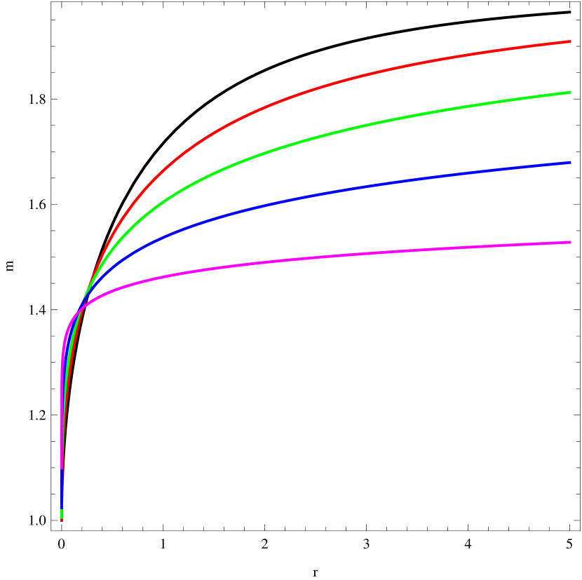
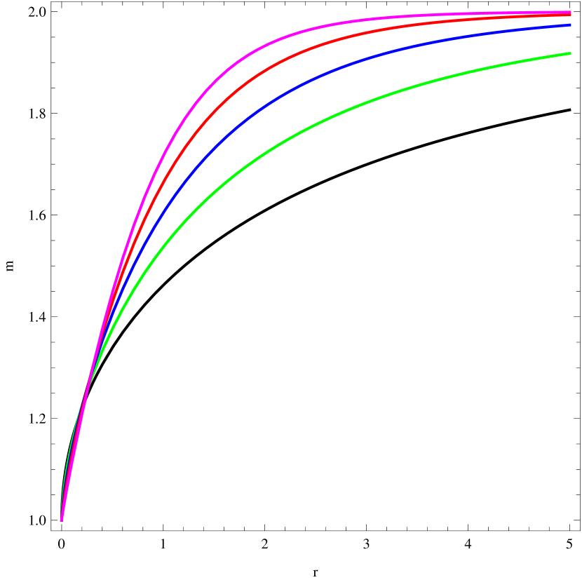
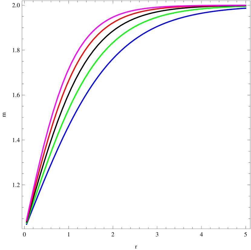
Figure 1: These figures show the evolution of the mass as the radius evolves for the case $n<0$, for instance $n=-0.5$ (left diagram); for the case $0<n<1$, for instance $n=0.5$ (middle diagram) and for the case $n>1$, for instance $n=2$ (right diagram). For the three diagrams, the representative of the $TT$ are the black ones $(b_{1}=0)$. The red, magenta, blue and green curves are plotted for $b_{1}=-2;-1;1;2$, respectively. The graphs here are related to neutron stars within polytropic EoS for power-law correction to $TT$.

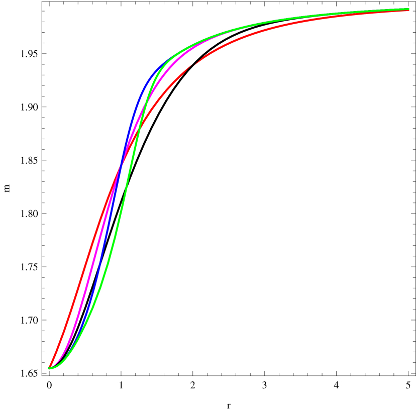
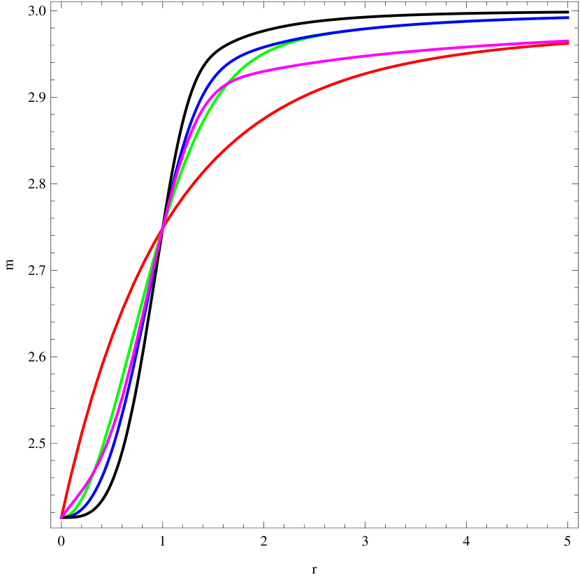
Figure 2: The figures show the evolution of the mass as the radius evolves for the case $q<0$, for instance $q=-1$ (left diagram) and for the case $q>0$, for instance $q=1$ (right diagram). For both diagrams, the representative of the $TT$ are the black ones $(b_{2}=0)$. The red, magenta, blue and green curves are plotted for $b_{2}=-1;-0.5;0.5;1$, respectively. The graphs here are related to neutron stars within polytropic EoS for exponential correction to $TT$.

2. SLy EoS

This type of equation of state characterizes the behaviour of nuclear matter at high densities and is expressed as

$$\zeta=\frac{a_{1}+a_{2}\xi+a_{3}\xi^{3}}{1+a_{4}\xi}f_{0}a_{5}\left(\xi-a_{6}\right)+f_{0}\left(a_{7}+a_{8}\xi\right)\left[a_{9}\left(a_{10}-\xi\right)\right]$$

$$+f_{0}\left(a_{11}+a_{12}\xi\right)\left[a_{13}\left(a_{14}-\xi\right)\right]+f_{0}\left(a_{15}+a_{16}\xi\right)\left[a_{17}\left(a_{18}-\xi\right)\right].$$ (25)

Here the parameters $\zeta$ and $\xi$ are defined as in (24) and the function $f_{0}$ is defined by

$$f_{0}(x)=\frac{1}{e^{x}+1}$$ (26)

The values of coefficients $a_{i}$ can be view in the Table $1$ [35].

Table 1
i	$a_{i}$(SLy)	i	$a_{i}$(SLy)
1	6.22	10	11.4950
2	6.121	11	-22.775
3	0.005925	12	1.5707
4	0.16326	13	4.3
5	6.48	14	14.08
6	11.4971	15	27.80
7	19.105	16	-1.653
8	0.8938	17	1.50
9	6.54	18	14.67

As in the previous case, we assume that the density at the center of star evolves from a critical $\rho_{c}$ to the total density at it surface. The deviation from the $TT$ is presented for the both power-law gravity and the exponential one for different values of the parameters $b_{1}$ and $b_{2}$. The evolution of the mass-radius diagram for neutron stars within SLy EoS are represented in Fig $3$ for power-law correction and Fig $4$ for exponential correction to the TT of gravity.

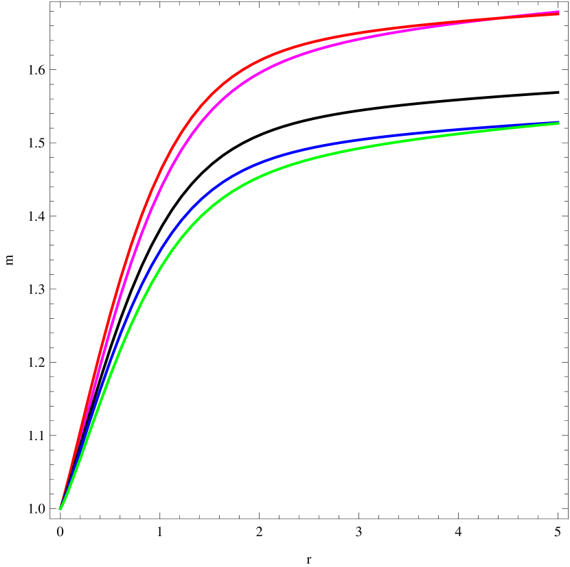
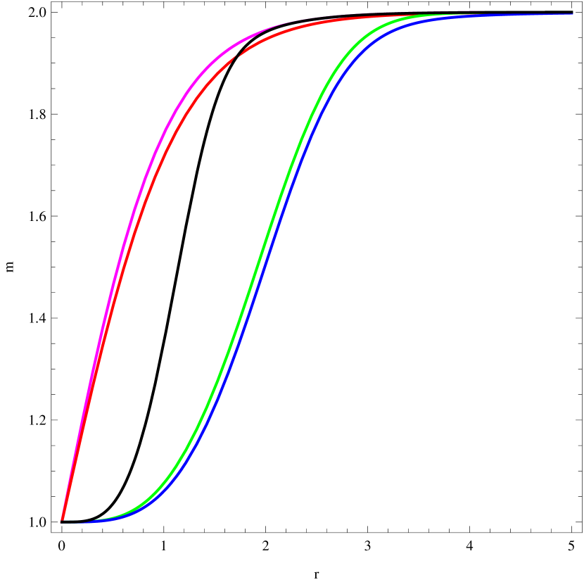
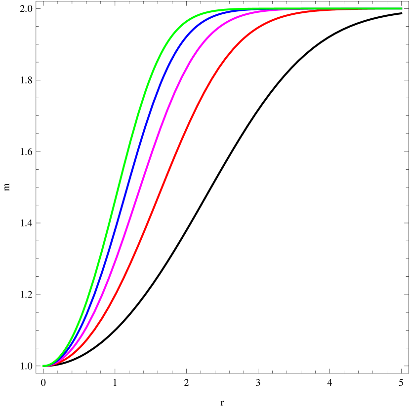
Figure 3: These figures show the evolution of the mass as the radius evolves for the case $n<0$, for instance $n=-0.5$ (left diagram); for the case $0<n<1$, for instance $n=0.5$ (middle diagram) and for the case $n>1$, for instance $n=2$ (right diagram). For the three diagrams, the representatives of the $TT$ are the black ones $(b_{1}=0)$. The red, magenta, blue and green curves are plotted for $b_{1}=-2;-1;1;2$, respectively. The graphs here are related to neutron stars within SLy EoS for power-law correction to $TT$.

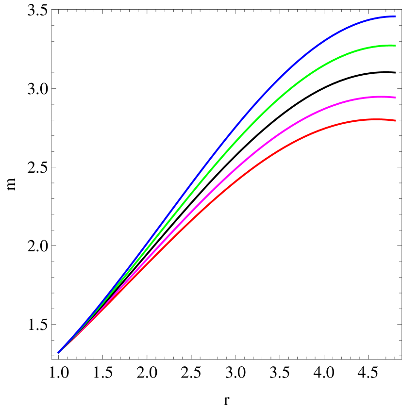
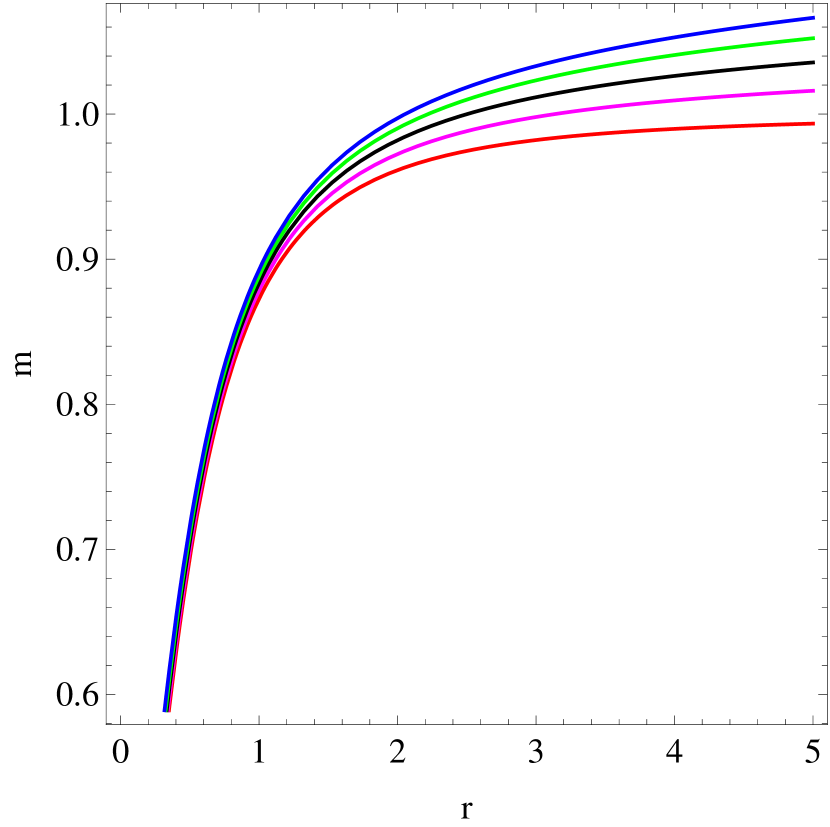
Figure 4: The figures show the evolution of the mass as the radius evolves for the case $q<0$, for instance $q=-1$ (left diagram) and for the case $q>0$, for instance $q=1$ (right diagram). For both diagrams, the representatives of the $TT$ are the black ones $(b_{2}=0)$. The red, magenta, blue and green curves are plotted for $b_{2}=-1;-0.5;0.5;1$, respectively. The graphs here are related to neutron stars within SLy EoS for exponential correction to $TT$.

3.1.2 Quark Stars

A quark star is a self-gravitating system consisting of deconfined $u$, $d$ and $s$ quarks and electrons [33]. These deconfined quarks are the fundamental elements of the color superconductor system. In the comparison with the standard hadron matter, they lead to a softer equation of state. In the frame of the so-called bag model, a simple equation of state is obtained for quark matter [34]

$$p=\omega(\rho-4\gamma)$$ (27)

where $\gamma$ is the bag constant. The value of the parameter $\omega$ depends on the mass $m_{s}$ of the strang quark. For the radiation, one has $m_{s}=0$ and the parameter is $\omega=0$, and for more realistic model where $m_{s}=250MeV$, the parameter is $\omega=0.28$. The parameter $\gamma$ belongs to the interval $58.8<B<91.2$ in the unit of $MeV/fm^{3}$ [11]. The evolution the mass-radius diagram for quark stars are represented in Fig $5$ for power-law correction and Fig $6$ for exponential correction to the TT of gravity.

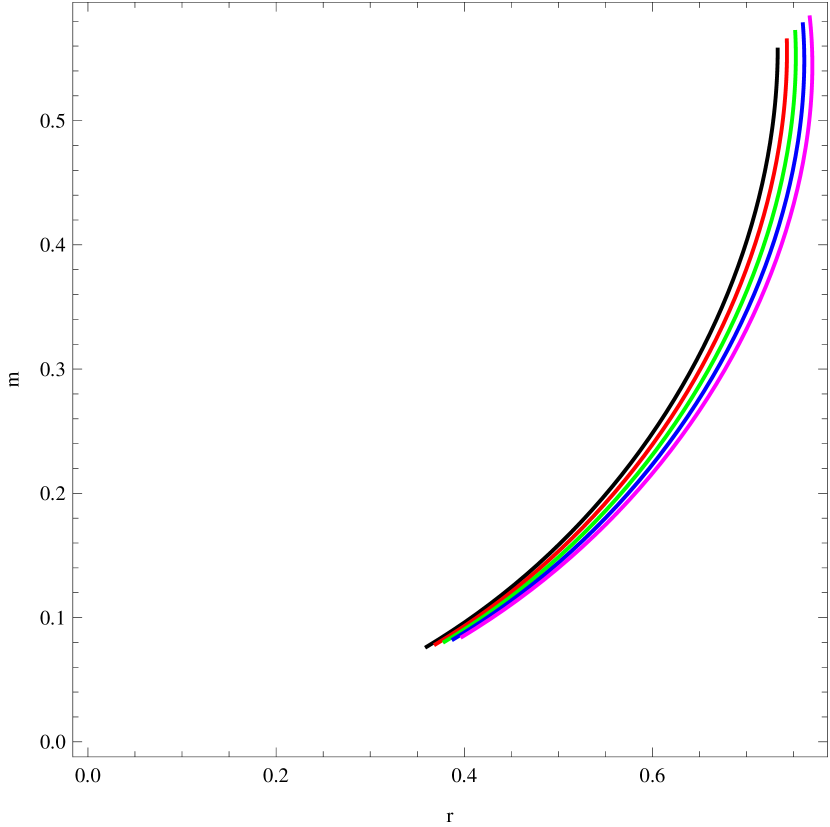
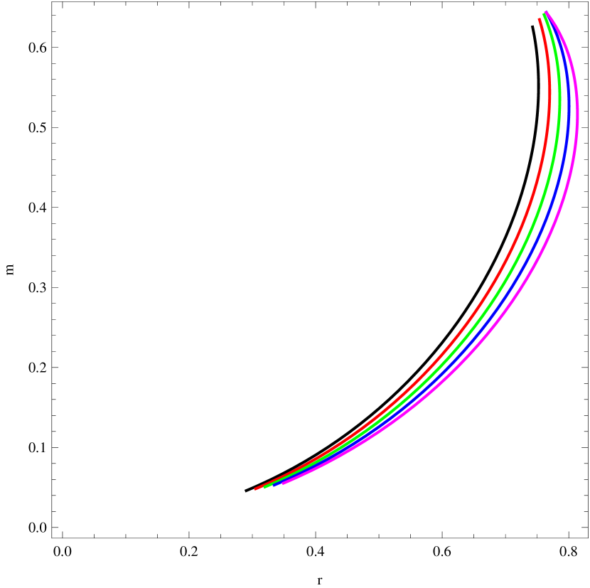
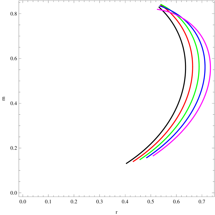
Figure 5: These figures show the evolution of the mass as the radius evolves for the case $n<0$, for instance $n=-0.5$ (left diagram); for the case $0<n<1$, for instance $n=0.5$ (middle diagram) and for the case $n>1$, for instance $n=2$ (right diagram). For the three diagrams, the representatives of the $TT$ are the black ones $(b_{1}=0)$. The red, magenta, blue and green curves are plotted for $b_{1}=-2;-1;1;2$, respectively. The graphs are related to the quark stars with the polytropic correction to TT.

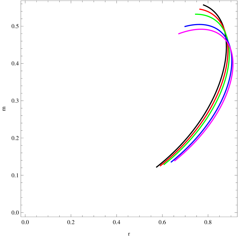
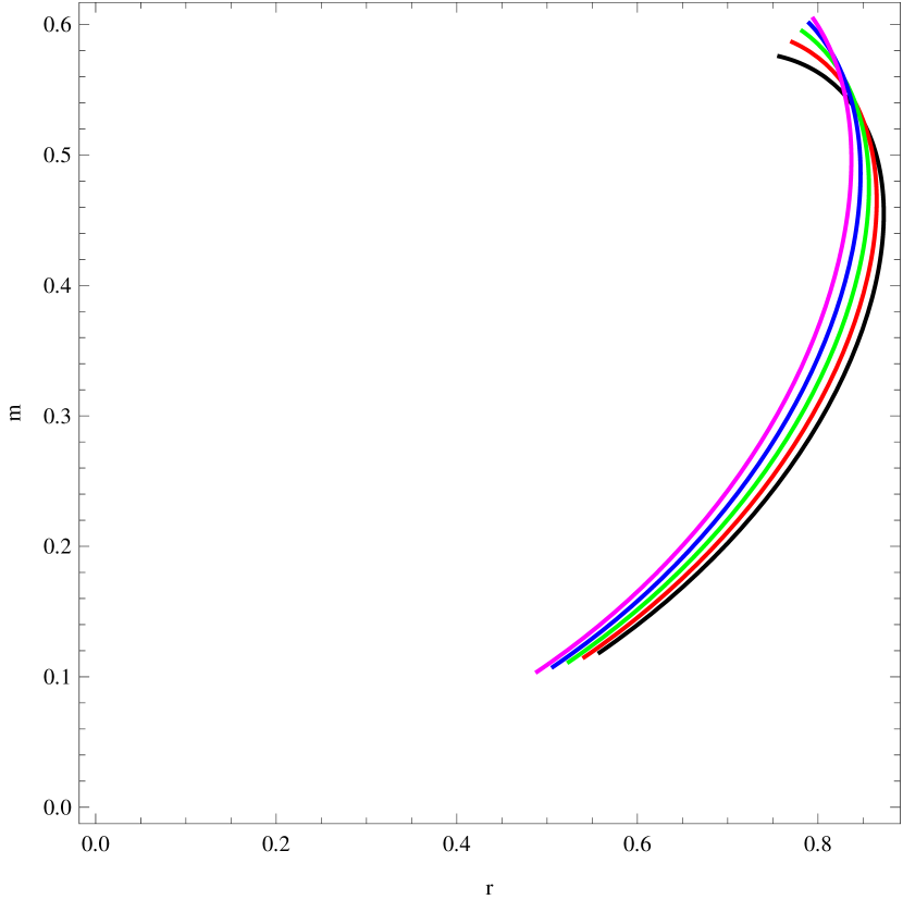
Figure 6: The figures show the evolution of the mass as the radius evolves for the case $q<0$, for instance $q=-1$ (left diagram) and for the case $q>0$, for instance $q=1$ (right diagram). For both diagrams, the representatives of the TT are the black ones ($b_{2}=0$). The red, magenta, blue and green curves are plotted for $b_{2}=-1;-0.5;0.5;1$, respectively. The graphs here are related to neutron stars within SLy EoS for exponential correction to TT.

4 Conclusion

The structures of neutron and quark stars structures have been analyzed in this work in the framework of $f(T)$, $T$ being the torsion scalar. The main goal here is searching the deviation of mass-radium diagram of both neutron and quark stars of the modified gravity, view as correction terms to the $TT$, from corresponding diagram of the $TT$. The first has been establishing the TOV equations for $f(T)$ theory. The fundamental fashion here is assuming the non-diagonal tetrad from which any constraint can occur about the choice of the algebraic action function. Therefore, we assume two interesting cases as correction terms; the power-law and exponential terms, including the parameters ($b_{1}$ and $n$) and ($b_{2}$ and $q$), respectively.

Our analysis are based on the numerical integration of the system formed by TOV equations and the different EoS, the polytropic and SLy EoS for neutron stars and a suitable EoS for the quark stars. Our results show that for some values of the input parameters in the neutron stars case, for both polytropic and SLy EoS, the deviation of the $f(T)$ terms from the TT is obvious for the beginning and the intermediate values of the radius. However, in some cases and for large values of the radius, the correction terms do not have effect on the evolution of the mass, with respect to the $TT$ case. In the quark stars case, it appears that for any value of the radius, the deviation of the $f(T)$ theory terms from the $TT$ is obvious.

Acknowledgments: A.V.Kpadonou and M.J.S.Houndjo thank Ecole Normale Supérieure de Natitingou for partial financial support. M.E.Rodrigues expresses his sincere gratitude do UFPA and CNPq for partial financial support during the elaboration of this work.

References

- [1]
- [2] A. S. Eddington, Mathematical Theory of Relativity (Cambridge University Press, Cambridge, 1923); H. Weyl, Annalen der Physik 364, 101 (1919).
- [3] A. Starobinsky, Physics Letters B 91, 99 (1980).
- [4] A. G. Riess et al. (Supernova Search Team), Astron.J. 116, 1009 (1998), arXiv:astro-ph/9805201 [astro-ph]; S. Perlmutter et al. (Supernova Cosmology Project), Astrophys. J. 517, 565 (1999), arXiv:astro-ph/9812133 [astro-ph].
- [5] T. P. Sotiriou and V. Faraoni, Rev.Mod.Phys. 82, 451 (2010), arXiv:0805.1726 [gr-qc].
- [6] A. De Felice and S. Tsujikawa, Living Reviews in Relativity 13, 3 (2010), arXiv:1002.4928 [gr-qc].
- [7] J. Khoury and A. Weltman, Phys. Rev. Lett. 93, 171104 (2004), arXiv:astro-ph/0309300 [astro-ph]; Phys. Rev. D 69, 044026 (2004), arXiv:astro-ph/0309411 [astro-ph].
- [8] P. Brax, C. van de Bruck, A.-C. Davis, and D. J. Shaw, Phys. Rev. D 78, 104021 (2008), arXiv:0806.3415 [astro-ph].
- [9] D. Psaltis, Living Reviews in Relativity 11 (2008), arXiv:0806.1531 [astro-ph].
- [10] C. Schimdt et al., Astron. Astrophys 463, 405 (2007).
- [11] D. N. Spergel et al. [WMAP Collaboration], Astrophys. J. Suppl. 148, 175 (2003) arXiv:astro-ph/0302209.
- [12] S. Capozziello, Int. J. Mod. Phys. D 11, 483 (2002).
- [13] S. Capozziello, S. Carloni, A. Troisi, Recent Res. Dev. Astron. Astrophys 1, 625 (2003).
- [14] S. Nojiri, S.D. Odintsov, Phys. Rev. D 68, 123512 (2003); Phys. Lett. B 576, 5 (2003).
- [15] S. M. Carroll, V. Duvvuri, M. Trodden and M. S. Turner, Phys. Rev. D. 70, 043528 (2004).
- [16] G. J. Olmo, Int.J.Mod.Phys. D 20, 413 (2011).
- [17] S. Nojiri and S. D. Odintsov, Phys. Rept. 505, 59 (2011) arXiv:1011.0544 [gr-qc]; eConf C 0602061, 06 (2006) Int. J. Geom. Meth. Mod. Phys. 4, 115 (2007)] [hep-th/0601213]; arXiv:1306.4426 [gr-qc].
- [18] S. Capozziello and V. Faraoni, Beyond Einstein Gravity (Springer) New York (2010).
- [19] S. Capozziello and M. De Laurentis, Phys. Rept. 509, 167 (2011) arXiv:1108.6266[gr-qc].
- [20] A. de la Cruz-Dombriz and D. Saez-Gomez, Entropy 14, 1717 (2012) arXiv:1207.2663 [gr-qc].
- [21] [22] S. Nojiri and S. D. Odintsov, Gen. Rel. Grav. 36, 1765 (2004), arXiv:hep-th/0308176 [hep-th].
- [22] M. B. Baibosunov, V. T. Gurovich, and U. M. Imanaliev, Soviet Journal of Experimental and Theoretical Physics 71, 636 (1990); A. Vilenkin, Phys. Rev. D 32, 2511 (1985); G. M. Shore, Annals of Physics 128, 376 (1980).
- [23] J.-Q. Guo and A. V. Frolov, (2013), arXiv:1305.7290 [astro-ph.CO].
- [24] Hamzeh Alavirad and Joel M. Weller, arXiv:1307.7977v2 [gr-qc]
- [25] M. Hamani Daouda, Manuel E. Rodrigues and M.J.S. Houndjo, Eur. Phys. J. C 72 (2012) 1890, arXiv:1109.0528 [physics.gen-ph].
- [26] M. Hamani Daouda, Manuel E. Rodrigues and M.J.S. Houndjo, Eur. Phys. J. C 71 (2011) 1817, arXiv:1108.2920 [astro-ph.CO].
- [27] E. Babichev and D. Langlois, Phys.Rev. D 81, 124051 (2010), arXiv:0911.1297 [gr-qc].
- [28] A. Cooney, S. DeDeo, and D. Psaltis, Phys.Rev. D 82, 064033 (2010), arXiv:0910.5480 [astro-ph.HE].
- [29] M. Orellana, F. Garcia, F. A. Teppa Pannia, and G. E. Romero, Gen. Relativ. Gravit. (2013), arXiv:1301.5189 [astro-ph.CO].
- [30] C. Deliduman, K. Eksi, and V. Keles, JCAP 1205, 036 (2012), arXiv:1112.4154 [gr-qc].
- [31] E. Santos, Astrophys. Space Sci. 341, 411 (2012), arXiv:1104.2140 [gr-qc].
- [32] F. Kamiab and N. Afshordi, Phys. Rev. D 84, 063011 (2011), arXiv:1104.5704 [astro-ph.CO].
- [33] J. Khoury and A. Weltman, Phys. Rev. D 69, 044026 (2004) astro-ph/0309411; J. Khoury and A. Weltman, Phys. Rev. Lett. 93, 171104 (2004) arXiv:astro-ph/0309300.
- [34] A. V. Astashenok, S. Capozziello and S. D. Odintsov, accepted for publication in Phys. Lett. B, arXiv:1412.5453 [gr-qc]
- [35] P. Haensel and A. Y. Potekhin, Astron. Astrophys. 428, 191 (2004), arXiv:astro-ph/0408324 [astro-ph].