Anisotropic Strange Quintessence Stars in $f(R)$ Gravity

Abstract

In this paper, we have formulated the new exact model of quintessence anisotropic star in $f(R)$ theory of gravity. The dynamical equations in $f(R)$ theory with the anisotropic fluid and quintessence field have been solved by using Krori-Barua solution. In this case, we have used the Starobinsky model of $f(R)$ gravity. We have determined that all the obtained solutions are free from central singularity and potentially stable. The observed values of mass and radius of the different strange stars PSR J 1614-2230, SAXJ1808.4-3658(SS1), 4U1820- 30, PSR J 1614-2230 have been used to calculate the values of unknown constants in Krori and Barua metric. The physical parameters like anisotropy, stability and redshift of the stars have been investigated in detail.

Keywords: $f(R)$ Theory of Gravity; Quintessence Field, Krori-Barua Metric.

PACS Numbers: 97.60.Jd; 12.60.-i; 04.50.Kd

1 Introduction

The discovery of cosmic acceleration is one the major advancements in modern cosmology. The observation of type Ia supernovae (SNe Ia) combined with observational probes of numerous mounting astronomical evidences like the cosmic microwave background (CMB), large scale structure surveys (LSS) and Wilkinson Microwave Anisotropy Probe (WMAP) (Perlmutter et al.1999, Spergel et al.2007, Hawkins 2003, Eisentein et al.2005) reveal that the cosmos at present is dominated by exotic energy component named as dark energy (DE). The investigation of current cosmic expansion and nature of DE has been widespread among the scientists. For this purpose, numerous efforts have been made based upon different strategies. These efforts can be grouped in two categories: introducing new ingredients of DE to the entire cosmic energy and modification of Einstein-Hilbert action to obtain modified theories of gravity such as $f(R)$ (Nojiri and Odintsov 2011) $f(\mathcal{T})$ (Ferraro and Fiorini 2007) where $\mathcal{T}$ being the torsion, $f(R,T)$ (Harko et al.2011) where $R$ and $T$ represent the scalar curvature and trace of the energy-momentum tensor, $f(R,T,R^{\mu\nu}T_{\mu\nu})$ (Haghani 2013) and Gauss-Bonnet gravities (Cognola 2006).

It has been the subject of great interest to study the models of anisotropic stars solutions during the last decades (Herrera and Santos 1997). Egeland (2007) investigated that the cosmological constant would exist due to density of the vacuum, this is consequence of modeling the mass and radius of the Neutron star. In order to prove this fact Egeland used the relativistic equation of hydrostatic equilibrium with fermion equation of state (EoS). As $f(R)$ model with constant $R$ gives cosmological constant, therefore motivated by this fact, we study the structure of strange stars and concluded that $f(R)$ gravity with model $f(R)=R+\lambda{R}^{2}$ (where $\lambda$ is constant) can describes the class of some anisotropic compact strange stars for example X-ray bruster 4$U$1820-30, X-ray pulsar Her X-1, Millisecond pulsar SAX J 1808-3658 etc. in a very scientific way. During the recent years, Dey et al.(1998), Usov (2004), Ruderman (1972), Mak and Harko (2002, 2003) have studied the physical properties of strange stars by using different approaches. Also, Herrera et al. (2008) have examined all static spherically symmetric solution of Einstein field equations and discussed the physical implication of these solutions.

The exact solutions have many applications in astronomy and astrophysics. For examples these can explain the properties and compositions of astrophysical objects. Mak and Harko (2004) presented a class of exact solutions of Einstein field equations with anisotropic source. The physical properties of these solutions imply that matter density as well as tangential and radial pressure are regular inside the compact star. Chaisi and Maharaj (2005) established a mathematical algorithm which explain the solution of the field equations for the anisotropic source. Rahaman et al.(2012) apply the Krori-Barua (1975) solution to the charged strange compact stars. Recently, Kalam et al.(2012) and Kalam et al.(2013) have studied the models of the compact objects using the Krori-Barua metric assumption. Hossein et al.(2012) discussed the anisotropic star model in the presence of varying varying cosmological constant. Bhar et al.(2015) investigated the higher dimensional compact star. This work has been extended by Maurya et al.(2014) for the charged anisotropic compact stars.

The study of compact stars such as relativistic massive objects have been the subject of interest in GR as well as in modified theories of gravity (Camenzind 2007, Abbas et al.2014, Abbas et al.2015a, 2015b, 2015c, 2015d, Sharif and Abbas 2013a, 2013b, Sharif and Zubair 2013a, 2013b). Being highly dense these are small in size and posses the extremely massive structure, and produce a strong gravitational field. Recently, there has been growing interest to study the compact stars in modified theories of gravity like $f(R)$ and $f(G)$. Particularly, Astashenok (2013), presented neutron stars solutions for viable models of $f(G)$ gravity. Motivated by this work, we study the compact stars solutions and their dynamical stability for a viable model of $f(R)$ gravity. We shall find the exact solutions for quintessence compact stars which are comparable with observational data. Our plan in this work is as follows: In Sec.2, we present basic equations of motion for $f(R)$ gravity. The analytic solution for the viable $f(G)$ model is presented in Sec.3. Sec.4 deals with the physical analysis of the given system. The last section summaries the results of the paper.

2 Model of Anisotropic Quintessence star in $f(R)$ Gravity

We assume that the manifold possesses a stationary and spherical symmetry for which the metric can be written as

$$ds^{2}=-e^{\mu(r)}dt^{2}+e^{\nu(r)}dr^{2}+r^{2}(d\theta^{2}+sin^{2}\theta{d\phi^{2}}),$$ (1)

where $\nu=Ar^{2}$, $\mu=Br^{2}+C$ Krori and Barua (1975), $A$, $B$ and $C$ are arbitrary constant to be evaluated by using some physical conditions.
$f(R)$ gravity is defined by the action

$$\mathcal{\mathcal{I}}=\int{dx^{4}\sqrt{-g}\left(f(R)+\mathcal{L}_{(matter)}\right)},$$ (2)

where $\kappa^{2}=1,f(R)$ is generic function of scalar curvature and $\mathcal{L}_{(matter)}$ determines the role of matter contents. Variation of action (1) with respect to $g_{\mu\nu}$ yields the field equations

$$G_{{\mu}{\nu}}=T_{{\mu}{\nu}}^{(curv)}+\mathcal{T}_{{\mu}{\nu}},$$ (3)

where $\mathcal{T}_{{\mu}{\nu}}=T_{{\mu}{\nu}}^{matter}+\mathcal{Q}_{{\mu}{\nu}}$, which contains of ordinary matter contribution and quintessence filed defined by the parameter $-1<\omega_{q}<-1/3$ (Bhar 2015). $\mathcal{T}_{{\mu}{\nu}}$ is scaled by a factor of $\frac{1}{f_{R}(R)}$ and $T_{{\mu}{\nu}}^{(curv)}$ denotes the contribution that arises from the curvature to the effective stress-energy tensor given by

$$T_{{\mu}{\nu}}^{(curv)}=\frac{1}{f_{R}(R)}\left[\frac{1}{2}g_{\mu\nu}(f(R)-Rf_{R}(R))+f_{R}(R)^{;{\alpha}{\beta}}(g_{\mu\alpha}g_{\nu\beta}-g_{\mu\nu}g_{\alpha\beta})\right],$$ (4)

where $f_{R}(R)$, denotes derivative with respect to the Ricci scalar $R$.

The components of $\mathcal{Q}^{\mu}_{\nu}$ are defined as (Bhar 2015) $\mathcal{Q}^{t}_{t}=\mathcal{Q}^{r}_{r}=-\rho_{q}$ and $\mathcal{Q}^{\theta}_{\theta}=\mathcal{Q}^{\phi}_{\phi}=\frac{1}{2}(3\omega_{q}+1)\rho_{q}$. To obtain some particular strange star models, we assume the anisotropic fluid in the interior of compact object and it is defined by

$$T^{m}_{\alpha\beta}=(\rho+p_{t})u_{\alpha}{u}_{\beta}-p_{t}g_{\alpha\beta}+(p_{r}-p_{t})v_{\alpha}{v}_{\beta},$$ (5)

where $u_{\alpha}=e^{\frac{\mu}{2}}\delta^{0}_{\alpha}$, $v_{\alpha}=e^{\frac{\nu}{2}}\delta^{0}_{\alpha}$, $\rho$, $p_{r}$ and $p_{t}$ correspond to energy density, radial and transverse pressures, respectively. The modified field equations corresponding to spacetime (4) lead to

$$\rho+\rho_{q}=-e^{-\nu}f_{RRR}+e^{-\nu}\left(\frac{\nu^{\prime}}{2}-\frac{2}{r}\right)f_{RR}+\frac{e^{-\nu}}{r^{2}}\left(\frac{\mu^{\prime\prime}r^{2}}{2}+\frac{\mu^{\prime 2}r^{2}}{4}-\frac{\mu^{\prime}\nu^{\prime}r^{2}}{4}\right.$$

$$+ \left.\mu^{\prime}r\right)f_{R}-\frac{1}{2}f,$$

$$p_{r}+\rho_{q}=e^{-\nu}\left(\frac{\mu^{\prime}}{2}+\frac{2}{r}\right)f_{RR}-\frac{e^{-\nu}}{r^{2}}\left(\frac{\mu^{\prime\prime}r^{2}}{2}+\frac{\mu^{\prime 2}r^{2}}{4}-\frac{\mu^{\prime}\nu^{\prime}r^{2}}{4}-\nu^{\prime}r\right)f_{R}$$

$$+ \frac{1}{2}f,$$

$$p_{t}+\frac{1}{2}(3\omega_{q}+1)\rho_{q}=-e^{-\nu}f_{RRR}+e^{-\nu}\left(\frac{\mu^{\prime}}{2}-\frac{\nu^{\prime}}{2}+\frac{1}{r}\right)f_{RR}-\frac{e^{-\nu}}{r^{2}}\left(\frac{\mu^{\prime}r}{2}\right.$$

$$- \left.\frac{\nu^{\prime}r}{2}-e^{\nu}+1\right)f_{R}+\frac{1}{2}f.$$ (8)

Herein, we choose the Starobinsky model of the form

$$f(R)=R+\lambda{R}^{2},$$ (9)

where $\lambda$ is an arbitrary constant. One can set $\lambda=0$ to find the results in GR. Herein, we set $\lambda=2km^{2}$.

For this model the equations (2)-(8) become

$$\rho+\rho_{q}=\frac{e^{-2\nu}}{8r^{4}}\{r^{4}\lambda\mu^{\prime 4}-2r^{3}\lambda\mu^{\prime 3}(-4+r\nu^{\prime})+r^{2}\lambda\mu^{\prime 2}(16+8r\nu^{\prime}-11r^{2}\nu^{\prime 2}+4r^{2}\mu^{\prime\prime}$$

$$+ 8r^{2}\nu^{\prime\prime})+4r^{2}\lambda\mu^{\prime}(-16r\nu^{\prime 2}+3r^{2}\nu^{\prime 3}+\nu^{\prime}(-4+9r^{2}\mu^{\prime\prime}-7r^{2}\nu^{\prime\prime})+2r(-2\mu^{\prime\prime}$$

$$+ 6\nu^{\prime\prime}-2r\mu^{\prime\prime\prime}+r\nu^{\prime\prime\prime}))+4(-2e^{\nu}{r}^{2}+2e^{2\nu}r^{2}-20\lambda+24e^{\nu}\lambda-4e^{2\nu}\lambda$$

$$+ 12r^{3}\lambda\nu^{\prime 3}-3r^{4}\lambda\mu^{\prime\prime 2}-r^{2}\lambda\nu^{\prime 2}(12+11r^{2}\mu^{\prime\prime})+8r^{2}\lambda\nu^{\prime\prime}+8r^{4}\lambda\mu^{\prime\prime}\mu^{\prime\prime}-16$$

$$\times r^{3}\lambda\mu^{\prime\prime\prime}+2r\nu^{\prime}(e^{\nu}{r}^{2}-8\lambda+16r^{2}\lambda\mu^{\prime\prime}-14r^{2}\lambda\nu^{\prime\prime}+6r^{3}\lambda\mu^{\prime\prime\prime})+8r^{3}\lambda\nu^{\prime\prime\prime}$$

$$- 4r^{4}\lambda\mu^{(iv)})\},$$

$$p_{r}-\rho_{q}=\frac{e^{-2\nu}}{8r^{4}}\{-r^{4}\lambda\mu^{\prime 4}-2r^{4}\lambda\mu^{\prime 3}\nu^{\prime}+r^{3}\lambda\mu^{\prime 2}(-24\nu^{\prime}+3r\nu^{\prime 2}+4r(\mu^{\prime\prime}-\nu^{\prime\prime}))$$

$$- 4(-2e^{\nu}{r}^{2}+2e^{2\nu}r^{2}+28\lambda-24e^{\nu}\lambda-4e^{2\nu}\lambda-12r^{2}\lambda\nu^{\prime 2}-16r^{2}\lambda\mu^{\prime\prime}$$

$$+ 8r^{3}\lambda\nu^{\prime}\mu^{\prime\prime}+r^{4}\lambda\mu^{\prime\prime 2}+16r^{2}\lambda\nu^{\prime\prime}-8r^{3}\lambda\mu^{\prime\prime\prime}+8r\mu^{\prime}(e^{\nu}{r}^{2}-8\lambda+3r^{2}\lambda\nu^{\prime 2}$$

$$+ 6r^{2}\lambda\mu^{\prime\prime}-r\lambda\nu^{\prime}(8+r^{2}\mu^{\prime\prime})-4r^{2}\lambda\nu^{\prime\prime}+r^{3}\lambda\mu^{\prime\prime\prime})\},$$

$$p_{t}+\frac{1}{2}(3\omega_{q}+1)\rho_{q}=\frac{e^{-\nu}}{8r^{4}}\{r^{4}\lambda\mu^{\prime 4}+2r^{3}\lambda\mu^{\prime 3}(2-3r\nu^{\prime})+r^{2}\mu^{\prime 2}(-32r\lambda\nu^{\prime}$$

$$+ 17r^{2}\lambda\nu^{\prime 2}+2(e^{\nu}{r}^{2}-8\lambda+6r^{2}\lambda\mu^{\prime\prime}-6r^{2}\lambda\nu^{\prime\prime}))-2r\mu^{\prime}(-38r^{2}\lambda\nu^{\prime 2}+6r^{3}\lambda\nu^{\prime 3}$$

$$+ r\nu^{\prime}(e^{\nu}{r}^{2}-24\lambda+28r^{2}\lambda\mu^{\prime\prime}-14r^{2}\lambda\nu^{\prime\prime})-2(e^{\nu}{r}^{2}-4\lambda+12e^{n}u\lambda+10r^{2}\lambda\mu^{\prime\prime}$$

$$- 14r^{2}\lambda\nu^{\prime\prime}+6r^{3}\lambda\mu^{\prime\prime\prime}-2r^{3}\lambda\nu^{\prime\prime\prime}))-4(12r^{3}\lambda\nu^{\prime 3}-11r^{4}\lambda\mu^{\prime\prime}\nu^{\prime 2}-5r^{4}\lambda\mu^{\prime\prime 2}$$

$$+ \mu^{\prime\prime}(-e^{\nu}r^{4}+8r^{2}\lambda+8r^{4}\lambda\nu^{\prime\prime})+r\nu(e^{\nu}{r}^{2}-28\lambda+12e^{\nu}\lambda+28r^{2}\lambda\mu^{\prime\prime}-28r^{2}\lambda\nu^{\prime\prime}$$

$$+ 12r^{3}\lambda\mu^{\prime\prime\prime})+4\lambda(-7+6e^{\nu}+e^{2\nu}-3r^{3}\mu^{\prime\prime\prime}+2r^{3}\nu^{\prime\prime\prime}-r^{4}\mu^{(iv)}))\}.$$ (12)

Using the relations of $\mu$ and $\nu$, we find the following relations

$$\rho+\rho_{q}=\frac{1}{r^{4}}e^{-2Ar^{2}}\{e^{2Ar^{2}}(r^{2}-2\lambda)+2(-5-3B^{2}r^{4}+6B^{3}r^{6}+B^{4}r^{8}$$

$$+ 12A^{3}r^{6}(2+Br^{2})-A^{2}r^{4}(40+68Br^{2}+11B^{2}r^{4})+A(-4r^{2}+48Br^{4}$$

$$+ 26B^{2}r^{6}-2B^{3}r^{8}))\lambda+e^{Ar^{2}}(-r^{2}+2Ar^{4}+12\lambda)\},$$

$$p_{r}-\rho_{q}=\frac{1}{r^{4}}e^{-2Ar^{2}}\{-e^{(}2Ar^{2})(r^{2}-2\lambda)+2(-7+11B^{2}r^{4}+2B^{3}r^{6}$$

$$- B^{4}r^{8}+3A^{2}r^{4}(2+Br^{2})^{2}-2Ar^{2}(4+16Br^{2}+9B^{2}r^{4}+B^{3}r^{6}))\lambda+e^{Ar^{2}}(r^{2}$$

$$+ 2Br^{4}+12\lambda)\},$$

$$p_{t}+\frac{1}{2}(3\omega_{q}+1)=\frac{1}{r^{4}}e^{-2Ar^{2}}\{-2(-7+6e^{Ar^{2}}+e^{2Ar^{2}})\lambda+16B^{3}r^{6}\lambda$$

$$+ 2B^{4}r^{8}\lambda-24A^{3}r^{6}(2+Br^{2})\lambda+2A^{2}r^{4}(28+74Br^{2}+17B^{2}r^{4})\lambda+B^{2}r^{4}$$

$$\times (e^{Ar^{2}}r^{2}+22\lambda)+2Br^{2}(-6\lambda+e^{Ar^{2}}(r^{2}+6\lambda))-Ar^{2}(4(-7+19Br^{2}$$

$$+ 25B^{2}r^{4}+3B^{3}r^{6})\lambda+e^{Ar^{2}}(r^{2}+Br^{4}+12\lambda))\}.$$ (15)

We have four unknown functions $\rho,p_{r},p_{t},\rho_{q}$, and three Eqs.(2)-(15). To find the explicit relations of these parameters, we assume a relation between radial pressure and energy density of the form

$$p_{r}=\alpha\rho,\quad 0<\alpha<1,$$ (16)

where $\alpha$ plays the role of equation of state parameter. This relation is the particular form of equation of state, the general form of this equation has been presented by Herrera and Barreto (2013).

After some manipulations and using Eq.(16), we get the expressions of $\rho,p_{r},p_{t},\rho_{q}$ in the following form

$$\rho = \frac{1}{1+\alpha}\left\{\frac{1}{r^{4}}e^{-2Ar^{2}}(8(-3-3Ar^{2}+(-7A^{2}+4AB+2B^{2})r^{4}+2(3A^{3}\right.$$ (17)

$$- \left.7A^{2}B+AB^{2}+B^{3})\times{r}^{6}+A(A-B)B(3A+B)r^{8})\lambda+2e^{Ar^{2}}((A\right.$$

$$+ \left.B)r^{4}+12\lambda))\right\},$$

$$\rho_{q} = \frac{1}{r^{4}(1+\alpha)}e^{-2Ar^{2}}\left\{e^{2Ar^{2}}(1+\alpha)(r^{2}-2\lambda)+2(7-5\alpha+12A^{3}r^{6}(2+Br^{2})\alpha\right.$$ (18)

$$+ \left.B^{2}r^{4}(-11-3\alpha+Br^{2}(-2+6\alpha+Br^{2}(1+\alpha)))-A^{2}r^{4}(12+40\alpha+Br^{2}\right.$$

$$\times \left.(12+68\alpha+Br^{2}(3+11\alpha)))+2Ar^{2}(4-2\alpha+Br^{2}(8(2+3\alpha)+Br^{2}(9\right.$$

$$- \left.Br^{2}(-1+\alpha)+13\alpha))))\lambda-e^{Ar^{2}}(r^{2}(1+\alpha)+2r^{4}(B-A\alpha)\right.$$

$$- \left.12(-1+\alpha)\lambda)\right\},$$

$$p_{r} = \frac{\alpha}{1+\alpha}\left\{\frac{1}{r^{4}}e^{-2Ar^{2}}(8(-3-3Ar^{2}+(-7A^{2}+4AB+2B^{2})r^{4}+2(3A^{3}\right.$$ (19)

$$- \left.7A^{2}B+AB^{2}+B^{3})\times{r}^{6}+A(A-B)B(3A+B)r^{8})\lambda+2e^{Ar^{2}}((A\right.$$

$$+ \left.B)r^{4}+12\lambda))\right\},$$

$$p_{t} = \frac{1}{2r^{4}(1+\alpha)}e^{-2Ar^{2}}\left\{-e^{2Ar^{2}}(1+\alpha)(\lambda(2-6\omega_{q})+r^{2}(1+3\omega_{q}))+e^{Ar^{2}}\right.$$

$$\times \left.(-2(A-B)Br^{6}(1+\alpha)+r^{2}(1+\alpha)(1+24(-A+B)\lambda+3\omega_{q})-12\lambda\right.$$

$$\times \left.(1+3\alpha+3(-1+\alpha)\omega_{q})-2r^{4}(A+A\alpha(2+3\omega_{q})-B(3+2\alpha+3\omega_{q})))\right.$$

$$- \left.2\lambda(-7-19\alpha+12Br^{2}(1+\alpha)+3(7-5\alpha)\omega_{q}+B^{4}r^{8}(1+\alpha)(-1+3\omega_{q})\right.$$

$$+ \left.2B^{3}r^{6}(-9-5\alpha+(-3+9\alpha)\omega_{q})-B^{2}r^{4}(33+25\alpha+(33+9\alpha)\omega_{q})\right.$$

$$+ \left.12A^{3}r^{6}(2+Br^{2})(2+3\alpha(1+\omega_{q}))+2Ar^{2}(-2(5+8\alpha+3(-2+\alpha)\omega_{q})\right.$$

$$+ \left.B^{3}r^{6}(7+5\alpha-3(-1+\alpha)\omega_{q})+2Br^{2}(27+31\alpha+12(2+3\alpha)\omega_{q})+B^{2}r^{4}\right.$$

$$\times \left.(59+63\alpha+3(9+13\alpha)\omega_{q}))-A^{2}r^{4}(4(17+9\omega_{q}+6\alpha(4+5\omega_{q}))+B^{2}r^{4}\right.$$

$$\times \left.(34+\alpha(45+33\omega_{q}))+Br^{2}(r^{2}(3+9\omega_{q})+4(40+54\alpha+(9+51\alpha)\omega_{q}))))\right\}.$$

The equation of state (EoS) parameters corresponding to radial and transverse directions can be obtained as

$$\omega_{r} = \alpha,$$ (21)

$$\omega_{t} = \left\{-e^{2Ar^{2}}(1+\alpha)(\lambda(2-6\omega_{q})+r^{2}(1+3\omega_{q}))+e^{Ar^{2}}(-2(A-B)Br^{6}(1\right.$$ (22)

$$+ \left.\alpha)+r^{2}(1+\alpha)(1+24(-A+B)\lambda+3\omega_{q})-12\lambda(1+3\alpha+3(-1+\alpha)\omega_{q})\right.$$

$$- \left.2r^{4}(A+A\alpha(2+3\omega_{q})-B(3+2\alpha+3\omega_{q})))-2\lambda(-7-19\alpha+12Br^{2}(1\right.$$

$$+ \left.\alpha)+3(7-5\alpha)\omega_{q}+B^{4}r^{8}(1+\alpha)(-1+3\omega_{q})+2B^{3}r^{6}(-9-5\alpha+(-3+9\alpha)\right.$$

$$\times \left.\omega_{q})-B^{2}r^{4}(33+25\alpha+(33+9\alpha)\omega_{q})+12A^{3}r^{6}(2+Br^{2})(2+3\alpha(1+\omega_{q}))\right.$$

$$+ \left.2Ar^{2}(-2(5+8\alpha+3(-2+\alpha)\omega_{q})+B^{3}r^{6}(7+5\alpha-3(-1+\alpha)\omega_{q})+2Br^{2}\right.$$

$$\times \left.(27+31\alpha+12(2+3\alpha)\omega_{q})+B^{2}r^{4}(59+63\alpha+3(9+13\alpha)\omega_{q}))-A^{2}r^{4}(4\right.$$

$$\times \left.(17+9\omega_{q}+6\alpha(4+5\omega_{q}))+B^{2}r^{4}(34+\alpha(45+33\omega_{q}))+Br^{2}(r^{2}(3+9\omega_{q})\right.$$

$$+ \left.4(40+54\alpha+(9+51\alpha)\omega_{q}))))\right\}/\left\{2(8(-3-3Ar^{2}+(-7A^{2}+4AB+2B^{2})r^{4}\right.$$

$$+ \left.2(3A^{3}-7A^{2}B+AB^{2}+B^{3})r^{6}+A(A-B)B(3A+B)r^{8})\lambda+2e^{Ar^{2}}((A\right.$$

$$+ \left.B)r^{4}+12\lambda))\right\}.$$

We show the evolution of energy density $\rho$, radial pressure $p_{r}$, tangential pressure $p_{t}$ and quintessence field $\rho_{q}$ for the strange star candidates Her X-1, SAX J 1808.4-3658 and 4U 1820-30 in Figures 1-4.

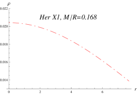
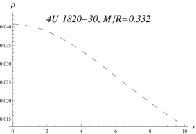
Figure 1: Evolution of energy density $\rho$ versus $r(km)$ at the stellar interior of strange star candidates. Herein, we set $\lambda=2km^{2}$, $\alpha=.01$ and $\omega_{q}=0.4$.

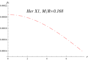
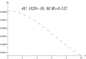
Figure 2: Evolution of radial pressure $p_{r}$ versus $r(km)$ at the stellar interior of strange star candidates.

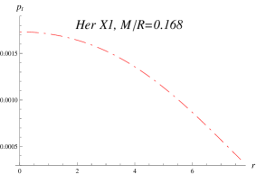
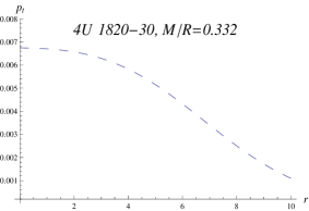
Figure 3: Evolution of transverse pressure $p_{t}$ versus $r(km)$ at the stellar interior of strange star candidates.

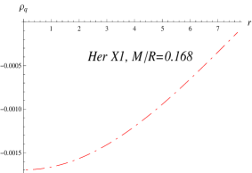
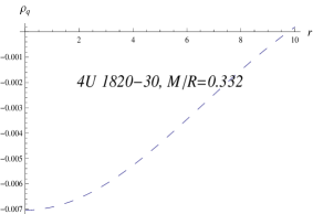
Figure 4: Evolution of transverse pressure $p_{t}$ versus $r(km)$ at the stellar interior of strange star candidates.

3 Physical Analysis

Here, we discuss some physical conditions which are necessary for the interior solution. In the following, we present the anisotropic behavior and stability conditions.

3.1 Anisotropic Constraints

Taking derivatives of equations (17) and (19) with respect to radial coordinate, we have

$$\frac{d\rho}{dr} = -\frac{1}{r^{5}(1+\alpha)}4e^{-2Ar^{2}}\left\{-24\lambda+4r^{2}(-9A-6A^{2}r^{2}-2(10A^{3}-11A^{2}B\right.$$ (23)

$$- \left.AB^{2}+B^{3})r^{4}+2A(6A^{3}-17A^{2}B+4AB^{2}+3B^{3})r^{6}+2A^{2}(A-B)\right.$$

$$\times \left.B(3A+B)r^{8})\lambda+e^{Ar^{2}}(A(A+B)r^{6}+12(2+Ar^{2})\lambda)\right\},$$

$$\frac{dp_{r}}{dr} = -\frac{1}{r^{5}(1+\alpha)}4e^{-2Ar^{2}}\alpha\left\{-24\lambda+4r^{2}(-9A-6A^{2}r^{2}-2(10A^{3}-11A^{2}B\right.$$ (24)

$$- \left.AB^{2}+B^{3})r^{4}+2A(6A^{3}-17A^{2}B+4AB^{2}+3B^{3})r^{6}+2A^{2}(A-B)\right.$$

$$- \left.B(3A+B)r^{8})\lambda+e^{Ar^{2}}(A(A+B)r^{6}+12(2+Ar^{2})\lambda)\right\}.$$

Similarly, one can find the second derivatives of $\rho$ and $p_{r}$. We present the evolution of $\frac{d\rho}{dr}$ and $\frac{dp_{r}}{dr}$ in Figures 5 and 6 which show that $\frac{d\rho}{dr}<0$ and $\frac{dp_{r}}{dr}<0$.

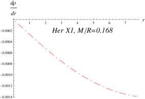
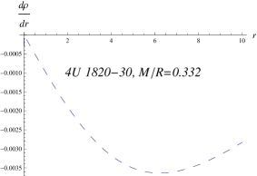
Figure 5: Evolution of $\frac{d\rho}{dr}$ versus $r(km)$ at the stellar interior of strange star candidates.

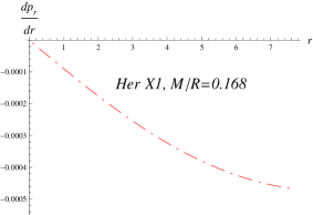
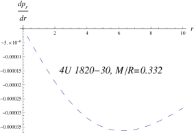
Figure 6: Evolution of $\frac{p_{r}}{dr}$ versus $r(km)$ at the stellar interior of strange star candidates.

One can explore the behavior of derivatives of $\rho$ and $p_{r}$ at center $r=0$ of compact star and it can be seen that

$$\frac{d\rho}{dr}=0,\quad\quad\frac{dp_{r}}{dr}=0,$$

$$\frac{d^{2}\rho}{dr^{2}}<0,\quad\quad\frac{d^{2}p_{r}}{dr^{2}}<0.$$ (25)

This indicate the maximality of central density and radial pressure. Hence $\rho$ and $p_{r}$ attain maximum values at $r=0$ and functional values decreases with the increase in $r$ as shown in Figures 1-2. From Eqs.(21) and (22), we have $\omega_{r}>0$ and $\omega_{t}<1$ as shown in Figure 7 for different strange stars.

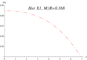
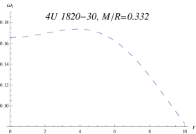
Figure 7: Evolution of of EoS parameter $\omega_{t}$ versus $r(km)$ at the stellar interior of strange star candidates.

The measure of anisotropy parameter $\Delta=\frac{2}{r}(p_{t}-p_{r})$ in this case is given by

$$\Delta = \frac{1}{r^{5}(1+\alpha)}e^{-2Ar^{2}}\left\{-e^{2Ar^{2}}(1+\alpha)(\lambda(2-6\omega_{q})+r^{2}(1+3\omega_{q}))+e^{Ar^{2}}(-2\right.$$ (26)

$$\times \left.(A-B)Br^{6}(1+\alpha)+r^{2}(1+\alpha)(1+24(-A+B)\lambda+3\omega_{q})-12\lambda(1\right.$$

$$+ \left.7\alpha+3(-1+\alpha)\omega_{q})-2r^{4}(A-3B(1+\omega_{q})+A\alpha(4+3\omega_{q})))-2\lambda(-7\right.$$

$$- \left.43\alpha+12Br^{2}(1+\alpha)+3(7-5\alpha)\omega_{q}-3B^{2}r^{4}(11+3\alpha)(1+\omega_{q})+B^{4}r^{8}\right.$$

$$\times \left.(1+\alpha)(-1+3\omega_{q})+6B^{3}r^{6}(-3+\alpha+(-1+3\alpha)\omega_{q})+12A^{3}r^{6}(2\right.$$

$$+ \left.Br^{2})(2+\alpha(5+3\omega_{q}))+2Ar^{2}(-2(5+14\alpha+3(-2+\alpha)\omega_{q})+B^{3}r^{6}(7\right.$$

$$+ \left.\alpha-3(-1+\alpha)\omega_{q})+6Br^{2}(9+13\alpha+4\times(2+3\alpha)\omega_{q})+B^{2}r^{4}(59+71\alpha\right.$$

$$+ \left.3(9+13\alpha)\omega_{q}))-A^{2}r^{4}(4(17+38\alpha+(9+30\alpha)\omega_{q})+B^{2}r^{4}\times(34+\alpha(61\right.$$

$$+ \left.33\omega_{q}))+Br^{2}(r^{2}(3+9\omega_{q})+4(40+82\alpha+(9+51\alpha)\omega_{q}))))\right\}.$$

Figure 8 shows the evolution of $\Delta$ for the different strange stars. It can be seen that $\Delta>0$, which implies that it is directed outward and repulsive force exists for these strange star models.

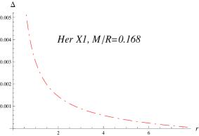
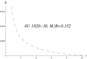
Figure 8: Variation of anisotropy measurement versus radial coordinate $r(km)$ at the stellar interior of strange star candidates.

3.2 Matching Conditions

Recently, Goswami et al.(2014), have proved that extra matching conditions that arise in the modified gravity imposes strong constraints on the stellar structure and thermodynamic properties. They showed that these constraints are non-physical. According to these authors, Schwarzschild solution is best choice in the exterior region for matching conditions. It means there does not exist general vacuum solution in $f(R)$ gravity as Schwarzschild solution in GR. Using this philosophy a lot of work in $f(R)$ gravity (Ganguly 2014, Ifra and Zubair 2015, Ifra et al.2015) has been done by taking the exterior solution as Schwarzschild or Vaidya metric.

Here, we match the interior metric (4) to the vacuum exterior spherically symmetric metric given by

$$ds^{2}=-\left(1-\frac{2M}{r}\right)dt^{2}+\left(1-\frac{2M}{r}\right)^{-1}dr^{2}+r^{2}d\theta^{2}+r^{2}sin^{2}{\theta}d\varphi^{2},$$ (27)

At the boundary surface $r=R$ continuity of the metric functions $g_{tt}$, $g_{rr}$ and $\frac{\partial g_{tt}}{\partial r}$ yield,

$$g_{tt}^{-}=g_{tt}^{+},~{}~{}~{}~{}~{}g_{rr}^{-}=g_{rr}^{+},~{}~{}~{}~{}~{}\frac{\partial g_{tt}^{-}}{\partial r}=\frac{\partial g_{tt}^{+}}{\partial r},$$ (28)

where $-$ and $+$, correspond to interior and exterior solutions. From the interior and exterior metrics, we get

$$A = -\frac{1}{R^{2}}ln\left(1-\frac{2M}{R}\right),$$ (29)

$$B = \frac{M}{R^{3}}{{\left(1-\frac{2M}{R}\right)}^{-1}},$$ (30)

$$C = ln\left(1-\frac{2M}{R}\right)-\frac{M}{R}{{\left(1-\frac{2M}{R}\right)}^{-1}}.$$ (31)

For the given values of $M$ and $R$ (Li 1999, Lattimer 2014) of the compact stars, the constants $A$ and $B$ are given in the table 1.

Table 1: Values of constants for given Masses and Radii of Stars

Strange Quark Star	$M$	$R(km)$	$\frac{M}{R}$	$A(km^{-2})$	$B(km^{-2})$
Her X-1	0.88$M_{\odot}$	7.7	0.168	0.006906276428	$0.004267364618$
SAX J 1808.4-3658	1.435$M_{\odot}$	7.07	0.299	0.01823156974	$0.01488011569$
4U 1820-30	2.25$M_{\odot}$	10.0	0.332	0.01090644119	$0.009880952381$

3.3 Energy Conditions

Energy constraints have many useful applications in GR as well as in modified gravity theories (discussion of various cosmological geometries). These inequalities are firstly formulated in the context of GR for the derivation of some general results involving strong gravitational fields. In GR, four types of energy constraints are formulated using a well-known geometrical results refereed as Raychaudhuri equation (explaining the dynamics of matter bits). These constraints are labeled as WEC, DEC, NEC and SEC. For an anisotropic fluid (5), these are defined as

$$\textbf{NEC}:\quad \rho+p_{r}\geq 0,\quad\rho+p_{t}\geq 0,$$

$$\textbf{WEC}:\quad \rho\geq 0,\quad\rho+p_{r}\geq 0,\quad\rho+p_{t}\geq 0,$$

$$\textbf{SEC}:\quad \rho+p_{r}\geq 0,\quad\rho+p_{t}\geq 0,\quad\rho+p_{r}+2p_{t}\geq 0,$$

$$\textbf{DEC}:\quad \rho>|p_{r}|,\quad\rho>|p_{t}|.$$

We find that our model satisfies these conditions for specific values of mass and radius which helps to find the unknown parameters for different strange stars. Here, we present the evolution of these conditions for strange star Her X-1 as shown in Figure 9. It can be seen that energy conditions are satisfied for our model.

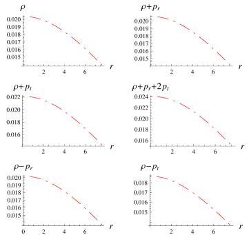
Figure 9: Evolution of energy constraints at the stellar interior of strange star Her X-1.

3.4 Stability Analysis

In this section, we discuss the stability of quintessence star models in $f(R)$ theory. To analyze the stability of our model we calculate the radial and transverse speeds as

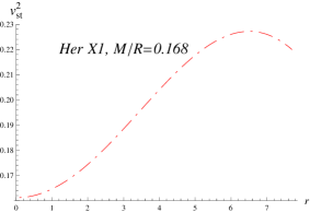
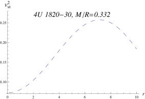
Figure 10: Variation of $v^{2}_{st}$ at the stellar interior of strange star candidates.

$$v^{2}_{sr} = \alpha,$$ (32)

$$v^{2}_{st} = \left\{-e^{2Ar^{2}}(1+\alpha)(4\lambda(1-3\omega_{q})+r^{2}(1+3\omega_{q}))-e^{Ar^{2}}(2A(A-B)Br^{8}(1\right.$$ (33)

$$+ \left.\alpha)+Ar^{4}(1+\alpha)(-1+24(A-B)\lambda-3\omega_{q})+24\lambda(1+3\alpha+3(-1\right.$$

$$+ \left.\alpha)\omega_{q})+2r^{6}(B^{2}(1+\alpha)-AB(4+3\alpha+3\omega_{q})+A^{2}(1+\alpha(2+3\omega_{q})))\right.$$

$$+ \left.r^{2}((1+\alpha)(-1-3\omega_{q})+12\lambda(-2B(1+\alpha)+A(3+5\alpha+3(-1+\alpha)\right.$$

$$\times \left.\omega_{q}))))-4\lambda(-7-19\alpha+6Br^{2}(1+\alpha)+3(7-5\alpha)\omega_{q}-B^{4}r^{8}(1+\alpha)\right.$$

$$\times \left.(-1+3\omega_{q})+B^{3}r^{6}(9+5\alpha+(3-9\alpha)\omega_{q})+12A^{4}r^{8}(2+Br^{2})(2+3\alpha\right.$$

$$\times \left.(1+\omega_{q}))+Ar^{2}(-17+12Br^{2}(1+\alpha)+33\omega_{q}+B^{4}r^{8}(1+\alpha)(-1+3\omega_{q})\right.$$

$$- \left.7\alpha(5+3\omega_{q})-4B^{2}r^{4}(23+22\alpha+3(5+4\alpha)\omega_{q})+4B^{3}r^{6}(-8-5\alpha\right.$$

$$+ \left.(-3+6\alpha)\omega_{q}))+A^{2}r^{4}(-4(5+8\alpha+3(-2+\alpha)\omega_{q})+2B^{3}r^{6}(7+5\alpha\right.$$

$$- \left.3(-1+\alpha)\omega_{q})+B^{2}r^{4}(19(8+9\alpha)+3(18+37\alpha)\omega_{q})+Br^{2}(r^{2}(3+9\omega_{q})\right.$$

$$+ \left.2(94+116\alpha+3(19+41\alpha)\omega_{q})))-A^{3}r^{6}(4(23+33\alpha+(9+39\alpha)\omega_{q})\right.$$

$$+ \left.B^{2}r^{4}(34+\alpha(45+33\omega_{q}))+Br^{2}(r^{2}(3+9\omega_{q})+4(46+63\alpha+(9+60\alpha)\right.$$

$$\times \left.\omega_{q}))))\right\}/\left\{4(-24\lambda+4r^{2}(-9A-6A^{2}r^{2}-2(10A^{3}-11A^{2}B-AB^{2}+B^{3})r^{4}\right.$$

$$+ \left.2A(6A^{3}-17A^{2}B+4AB^{2}+3B^{3})r^{6}+2A^{2}(A-B)B(3A+B)r^{8})\lambda\right.$$

$$+ \left.e^{Ar^{2}}(A(A+B)r^{6}+12(2+Ar^{2})\lambda))\right\}.$$

In the past, Herrera and his collaborators (Herrera 1992, Chan et al.1993, Di Prisco 1997)have developed a new technique to explore the potentially unstable matter configuration and introduced the concept of cracking. One can analyze the potentially stable and unstable regions regions depending on the difference of sound speeds, the region for which radial sound speed is greater than the transverse sound speed is said to be potentially stable. We find that radial sound speed is constant (Eq.(32)) and plot the transverse sound speed in Figure 10. It can be seen that $v^{2}_{st}$ satisfy the relation of stable matter configuration $0\leq{v}^{2}_{st}\leq 1$. This variation is further confirmed in Figure 11, where difference of the two sound speeds, i.e., $v^{2}_{st}-v^{2}_{sr}$ retain similar sign within the specific configuration and it satisfies the inequality $|v^{2}_{st}-v^{2}_{sr}|\leq 1$. Thus, our proposed strange star model is stable.

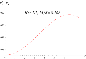
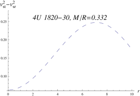
Figure 11: Variation of $v^{2}_{st}-v^{2}_{sr}$ at the stellar interior of strange star candidates.

3.5 Surface Redshift

The compactness of the star is given by

$$u = \frac{M(R)}{R}=\frac{1}{8(AR^{2})^{5/2}(1+\alpha)}R^{2}e^{-2AR^{2}}\pi\left\{-4\sqrt{A}(9B^{3}R^{2}\lambda+48A^{4}R^{4}(2\right.$$ (34)

$$+ \left.BR^{2})\lambda-4A^{3}R^{2}(10+BR^{2}(41+8BR^{2}))\lambda+2ABR^{2}(4e^{AR^{2}}+B(13\right.$$

$$+ \left.6BR^{2})\lambda)+A^{2}(-(192+BR^{2}(59+8BR^{2}(1+2BR^{2})))\lambda+8e^{AR^{2}}(R^{2}\right.$$

$$+ \left.24\lambda)))-e^{2AR^{2}}\sqrt{\pi}R(16A(-A-B+48A^{2}\lambda)\text{Erf}[\sqrt{A}R]-\sqrt{2}(536A^{3}\right.$$

$$- \left.59A^{2}B+26AB^{2}+9B^{3})\lambda\text{Erf}[\sqrt{2}\sqrt{A}R])\right\}.$$

The surface redshift ($Z_{s}$) corresponding to compactness (34) is given by

$${1+Z_{s}} = (1-2u)^{-1/2}=\{1-\frac{R^{2}e^{-2AR^{2}}\pi}{4(AR^{2})^{5/2}(1+\alpha)}\left\{-4\sqrt{A}(9B^{3}R^{2}\lambda+48A^{4}R^{4}(2\right.$$ (35)

$$+ \left.BR^{2})\lambda-4A^{3}R^{2}(10+BR^{2}(41+8BR^{2}))\lambda+2ABR^{2}(4e^{AR^{2}}+B(13\right.$$

$$+ \left.6BR^{2})\lambda)+A^{2}(-(192+BR^{2}(59+8BR^{2}(1+2BR^{2})))\lambda+8e^{AR^{2}}(R^{2}\right.$$

$$+ \left.24\lambda)))-e^{2AR^{2}}\sqrt{\pi}R(16A(-A-B+48A^{2}\lambda)\text{Erf}[\sqrt{A}R]-\sqrt{2}(536A^{3}\right.$$

$$- \left.59A^{2}B+26AB^{2}+9B^{3})\lambda\text{Erf}[\sqrt{2}\sqrt{A}R])\right\}\}^{-1/2}.$$

In Figure 12, we show the evolution of redshift for the strange star Her X-1.

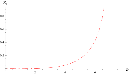
Figure 12: Evolution of redshift of strange star Her X-1.

4 Conclusion

The current cosmological observations imply that there are two phases of accelerated expansion in our present model of universe: cosmic inflation in the past era of the universe and acceleration in the present expansion of the universe. The investigation of current cosmic expansion and nature of dark energy has been widely accepted among the huge community of the scientists. For this purpose, several attempts have been made for the different strategies to modify the General Relativity. The $f(R)$ gravity is one of the modifications of General Relativity.

The current paper deals with the investigation of analytical models of quintessence compact stars with the anisotropic gravitating static source in the framework of $f(G)$ gravity. To this end, we have choosen the Starobinsky model of the form $f(R)=R+\lambda{R}^{2},$ further the stars are assumed as anisotropic in their internal structure. The analytic solution in $f(R)$ gravity have found by matching the interior spacetime with the well-known exterior vacuum spacetime. This matching is suitable in this case as $f(T)$ and GR both involve second order derivative terms in the equations of motion and we have continuity of metric coefficients up to first order derivatives. The graphical behavior of the results exhibit the some prominent properties of the anisotropic quintessence compact stars in $f(R)$ gravity.

We have evaluated the matter density, radial and transverse pressures, quintessence energy density and anisotropic parameter of the model. Using the observational data of SAXJ1808.4-3658(SS1)(radius=7.07 km),4U1820- 30 (radius=10 km), Her X-1 (radius=7.7 km), we have plotted the energy density, pressure and quintessence density at center $r=0$ to the boundary of the corresponding star. All this results have been shown in figure 1-4. The first and second derivatives of density and pressures shown in figures 5,6, indicate that these quantities have maximum values at the center and minimum values at boundary. The graphical behavior of quintessence density $\rho_{q}$ does not change in $f(R)$ theory of gravity as compared to GR, but there occur a deviation in numerical values 4. The constraint on the EoS parameter is given by $0<{\omega}_{t}<1$ (as shown in figure 7) which is in agreement with normal matter distribution in $f(R)$ gravity. We have investigated that for our model $\Delta>0$ (as shown in figure 8) and a repulsive force due to anisotropy results to the formation of more massive stars. The proposed model satisfy the energy conditions, as an example we have shown in figure 9 that these conditions are satisfied for $Her-X1(radius=7.7km)$. We have shown that $v_{st}^{2}<1$ (see figure 10) and $v_{st}^{2}>v_{sr}^{2}$ (see figure 11), hence our model is potentially stable. The range of surface redshift $Z_{s}$ for compact star candidate $Her-X1(radius=7.7km)$ is shown in figure 12.

5 Conflict of Interest

The authors declare that there is no conflict of interest regarding the publication of this work.

References

• [1] Abbas, G., Nazeer, S., Meraj,M. A.: Astrophys. Space Science 354, 449(2014)
• [2] Abbas, G., Kanwal, A., Zubair, M.: Astrophys. Space Science 357, 109(2015a)
• [3] Abbas, G. et al.: Astrophys. Space Science 357, 158(2015b)
• [4] Abbas, G., S. Qaisar, Meraj, M. A.: Astrophys. Space Science 357, 156(2015c)
• [5] Abbas, G., Zubair, M.: Anisotropic Compact Stars in $f(R)$ gravity (Submitted 2015)
• [6] Astashenok. A.Β V.Β , Capozziello. S.Β , Odintsov. S.Β D.Β , JCAP 1312, 040 (2013)
• [7] Bhar. P. , et al.: arXiv:1503.03439
• [8] Maurya. S.K. , et al.: arXiv:1408.5126
• [9] Camenzind. M. , ”Compact Objects in Astrophysics”, Springer-Verlag Berlin Heidelberg (2007)
• [10] Chaisi, M. and Maharaj S.D.: General Relativ. Gravit. 37, 1177(2005)
• [11] Cognola, G., et al.: Phys. Rev. D 73, 084007(2006)
• [12] Chan, R. Herrera, L. and Santos, N.O.: MNRAS 265, 533(1993)
• [13] Di Prisco, A. Herrera, L. and Varela, V.: Gen. Relativ. Grav. 29, 1239(1997)
• [14] Dey, M. et al.: Phys. Lett. B. 438, 1239(1998)
• [15] Eisentein, D.J. et al.: Astrophys. J. 633, 560(2005)
• [16] Egeland,E. Compact Stars (Trondheim, Norway, 2007)
• [17] Ferraro, R. and Fiorini, F.: Phys. Rev. D 75, 084031(2007)
• [18] Ganguly, A. et al.: Phys. Rev. D89, 064019(2014)
• [19] Goswami et al.:Phys. Rev. D90, 084011(2014)
• [20] Herrera, L.: Phys. Lett. A, 165, 206(1992)
• [21] Herrera, L and Santos,N.O.: Phys.Report.286, 53(1997)
• [22] Herrera, L. and Barreto, W.: Phys. Rev. D88, 084022(2013) Herrera, L., Ospino, J. and Di Prisco, A.: Phys. Rev. D77, 027502,(2008)
• [23] . Harko,T., Lobo, F.S.N., Nojiri, S. and Odintsov, S.D.: Phys. Rev. D 84, 024020(2011)
• [24] Haghani, Z., Harko, T., Lobo, F.S.N., Sepangi, H.R. and Shahidi, S.: Phys. Rev. D 88, 044023(2013)
• [25] Hossein. Sk. M. et al., Int. J. Mod. Phys. D21, 1250088(2012)
• [26] Hawkins, E. et al.: Mon. Not. Roy. Astron. Soc. 346, 1250088(2003)
• [27] Ifra, N. and Zubair, M.: Eur.Phys.J. C75, 62(2015)
• [28] Ifra, N. et al. : JCAP1502, 033(2015)
• [29] Krori K.D. and Barua, J.: J. Phys. A.: Math. Gen.8, 508(1975)
• [30] Kalam. M, et al.: Eur. Phys. J. C72, 2248(2012)
• [31] Kalam. M, et al.: Eur. Phys. J. C73, 2409(2013)
• [32] Lattimer . J.Β M.Β and Steiner. A.Β W.Β , Astrophys.Β J.Β  784, 123(2014)
• [33] Li, X.Β D.Β , Bombaci. I.Β , Dey. M.Β , Dey. J.Β  and van den Heuvel. E.Β P.Β J.Β , Phys.Β Rev.Β Lett.Β  83, 3776(1999)
• [34] Mak, M.K. and Harko, T.: Chin. J. Astron. Astrophys. 2, 248(2002)
• [35] Mak, M.K. and Harko, T.: Proc. R. Soc. Lond. 459, 393(2003)
• [36] Mak, M.K. and Harko, T.: Int. J. Mod. Phys. D 13, 149(2004)
• [37] Nojiri, S. and Odintsov, S. D.: Phys. Rep. 505, 59(2011)
• [38] Bamba, K. Capozziello, S. Nojiri, S. and Odintsov, S.D.: Astrophys. Space Sci. 345, 155(2012)
• [39] Perlmutter, S. et al.: Astrophys. J. 517, 556(1999)
• [40] Riess, A.G. et al.: Astrophys. J. 659, 98(2007)
• [41] Ruderman, R.: Ann. Rev. Astron. Astrophys. 10, 427(1972)
• [42] Rahaman, F. et al.: Eur. Phys. J. C 72, 2071(2012)
• [43] Sharif. M.Β  and Abbas. G.Β , Eur.Β Phys.Β J.Β Plus 128, 102(2013)
• [44] Sharif. M.Β  and Abbas. G.Β , J. Phys. Soc. Jpn.textbf82, 034006(2013)
• [45] Sharif, M. and Zubair, M.: JCAP 11, 042(2013)
• [46] Sharif, M. and Zubair, M.: J. High Energy Phys. 12, 079(2013)
• [47] Spergel, D.N. et al.: Astrophys. J. Suppl. Ser. 170, 377(2007)
• [48] Usov, V.V.: Phys. Rev. D 70, 067301(2004)
• [49]