Electron dynamics in the normal state of cuprates: spectral function, Fermi surface and ARPES data

Abstract

An influence of the electron-phonon interaction on excitation spectrum and damping in a narrow band electron subsystem of cuprates has been investigated. Within the framework of the t-J model an approach to solving a problem of account of both strong electron correlations and local electron-phonon binding with characteristic Einstein mode $\omega_{0}$ in the normal state has been presented. In approximation Hubbard-I it was found an exact solution to the polaron bands. We established that in the low-dimensional system with a pure kinematic part of Hamiltonian a complicated excitation spectrum is realized. It is determined mainly by peculiarities of the lattice Green’s function. In the definite area of the electron concentration and hopping integrals a correlation gap may be possible on the Fermi level. Also, in specific cases it is observed a doping evolution of the Fermi surface. We found that the strong electron-phonon binding enforces a degree of coherence of electron-polaron excitations near the Fermi level and spectrum along the nodal direction depends on wave vector module weakly. It corresponds to ARPES data. A possible origin of the experimentally observed kink in the nodal direction of cuprates is explained by fine structure of the polaron band to be formed near the mode -$\omega_{0}$.

I Introduction

A description of the strongly correlated electron dynamics in cuprates is one of the intrigue task in the theory of condensed matter physics. The history of investigations from the beginning of the discovery HTSC covers a considerable quantity of publications. Experimental tunnel, magnetic, resonance and ARPES data 1 ; 2 ; 3 of pointed objects reflect the extremely complicated character of the interplay between charge, spin and lattice degrees of freedom. In spite of a wide experimental material as well as undoubted successful description of the cuprate electron structure by ab initio methods 4 ; 5 the series of observed phenomena to be connected with the strong electron correlations and electron-phonon interaction is not reproduced theoretically. In our opinion the reason is that within framework of such approaches it is impossible to extract an effective self-consistent field by analogy with Weiss field in magnetism or unperturbed Hamiltonian for free electrons in metals as well as the restricted statistics and difficulties to account for hole states. In some cases authors use the methods of metal physics especially to build the HTSC model and to account for strong electron-phonon interactions that is not useful for electron systems with strong correlations 6 ; 7 ; 8 . One of the puzzle phenomenon which is not described by existing theories is low-energy kink experimentally observed in the nodal dispersion of various cuprate materials 9 ; 10 ; 11 . Below we will give a theory which explains the origin of pointed anomaly and presents the consecutive picture of the strongly correlated electron dynamics in cuprates.

In this connection it is necessary to point out that the aim of this work is to build successive approximations for a diagrammatic method when the Hubbard-I 12 approximation is the starting point for any calculations. In this case we have a self-consistent field with the aid of which one can account for a specific character of doped Mott insulators. Indeed, below we will see the fundamental difference between metals and doped cuprates resulting in a strong correlation narrowing of the valence band for hole doping 13 ; 14 . Within the framework of the t-J model for lower Hubbard band without exchange electron interaction it easy to detect that in paramagnetic phase (PM) there are two noninteracting electron liquids with spin up and down avoiding one another and being in equilibrium. Hence, it gives rise to correlation effect. Indeed, unlike metals here every electron hopping does not change a number of electrons for both sites with spin-up and spin-down, respectively. In metal every electron hopping gives site with double occupancy changing the fixed electron quantity in the pointed subsystems. That’s why we must consider the whole electron system regardless of the spin. As a result in PM phase of doped Mott insulators in the limit of Coulomb repulsion $\textit{U}=\infty$ the excitation spectrum will be two-fold degenerate and chemical potential in the limit of half band filling is equal approximately to half of metal. It is necessary to point out that the ferromagnetically ordered strongly correlated electron system is similar to ordinary metal because in this case the Fermi statistic is working first of all.

Taking the strong electron-phonon interaction into account presents one of the most complicated task in the theory of condensed state. To solve this problem in a given work it is suggested to consider the Holstein model with one characteristic optical Einstein mode. The extension to case of few modes does not present any difficulties. To solve problem we use the method of inverse function to be formulated by us in work 15 for building the HTSC theory. Also, in contrast to existing theories 16 ; 17 where account of the electron-phonon interaction can not be exact our model based on transformation of Lang-Firsov 18 allows to solve this problem exactly. In this work in the Hubbard-I approximation first it has been shown how a strong electron-phonon binding modifies the band spectrum, chemical potential and Fermi surface. To calculate the Green’s function we used a such type of the Dyson’s equation when the self-energy depends on frequency only and all inhomogeneity is related exceptionally to the Fourier representation of the hopping integral.

Based on the diagrammatic contributions related to inelastic electron scattering a new specific of the electron spectrum and spectral density is revealed when the frequency and wave characteristic are varied abruptly through a small range. It is in a good qualitative agreement with the ARPES data. This circumstance makes the Fermi surface detection difficult and in specific cases points out the non-Fermi liquid behaviour of the electron ensemble.

The structure of the paper is as follows. In section 2 the starting fermion-boson Hamiltonian of the cuprate system is considered. It was diagonalized by unitary transformation. In approximation Hubbard-I a detailed analysis of the dynamic electron properties is carried out by taking into account an influence of the electron-phonon interaction, next nearest neighbours and changing the Fermi surface topology. In section 3 the low-dimensional correlations and electron-phonon interactions are included to provide the most general expression for Matsubara Green functions in the first nonvanishing approximation of time-dependent perturbation theory with respect to the inverse effective radius of interaction r $\approx$ 1/z, where z is the number of nearest neighbor in the simple square lattice. It was obtained the equations for excitation spectrum and damping. Also, the numerical analysis for chemical potential, Fermi surface, frequency spectrum and spectral density of the PM phase at value of parameter of electron-phonon binding g=0 was carried out. The polaron bands, spectral densities and their modifications versus parameter g were calculated. In conclusion we give the theoretical results having regard to the most typical experimental data.

II Holstein polarons and effective self-consistent field in cuprates

II.1 Hamiltonian of the fermion-bosonic system

To describe the electron dynamics it is necessary to calculate the Matsubara electron Green’s function poles of which determine an excitation spectrum $\omega_{\textbf{{k}}}$. Also, spectral density A($\omega$,k) is proportional to the square power of the imaginary part of Green’s function. In what follows we will consider a PM phase in which the spin index $\sigma$ does not play any role. The t-J model is believed to be the most simple for a description of the strong electron correlations. Apparently, in our case the exchange part of Hamiltonian is not considered. We add to Hamiltonian of t-J model the part used in the Holstein model of small polarons for the HTSC systems that are characterized by sufficiently strong electron-phonon interaction. These polarons are formed due to interaction between electrons and lattice optical vibrations. For simplicity, it is considered the Einstein model with phonon frequency $\omega_{0}$. Thus, the Hamiltonian is written as

$$\hat{H}=\hat{H}_{0}+V\,,$$ (1)

where

$$\begin{array}[]{l}\hat{H}_{0}=\hat{H}_{0f}+\hat{H}_{b}\\ {\hat{V}=-\sum\limits_{i,j,\sigma}t_{ij}c_{\sigma i}^{+}c_{\sigma j}(1-n_{i-\sigma})(1-n_{j-\sigma})}\\ {\hat{H}_{0f}=-\mu\sum\limits_{i,\sigma}n_{i\sigma}}\\ {\hat{H}_{b}=-g\sum\limits_{i}n_{i}\left(b_{i}^{+}+b_{i}\right)+\omega_{0}\sum\limits_{i}b_{i}^{+}b_{i}}\end{array}$$ (6)

Here, the fermionic $\hat{H}_{0f}$ and bosonic $\hat{H}_{b}$ terms are related to energy of chemical potential $\mu$ and local electron-phonon interaction in phonon subsystem with frequency $\omega_{0}$, respectively. The sum of these terms $\hat{H}_{0f}$ and $\hat{H}_{b}$ is considered as unperturbed Hamiltonian $\hat{H}_{0}$. For weakly doped cuprates $\hat{V}$ operator is taken as the perturbation, where both $c_{\sigma i}^{+}\;(c_{\sigma i})$ and $b_{i}^{+}\;(b_{i})$ create (annihilates) an electron of spin $\sigma$ and phonon on lattice site i, respectively, and $\textit{t}_{ij}$ is the hopping integral. $n_{i}=n_{i\sigma}+n_{i-\sigma}$is the site electron concentration, where $n_{i\sigma}$ represents the concentration of electrons on site i with spin $\sigma$. The exchange term of the Hamiltonian is neglected for the system in PM state.

The Lang-Firsov unitary transform 18 allows to separate the boson and fermion operators in $\hat{H}_{b}$. Then the transformed $\hat{H}_{b}$ takes the form $\hat{\tilde{H}}_{b}$:

$$\hat{\tilde{H}}_{b}=\omega_{0}\sum\limits_{i}b_{i}^{+}b_{i}-\xi\sum\limits_{i}n_{i}\,,$$ (7)

where $\xi=g^{2}/\omega_{0}$ is the polaron binding energy. Also, perturbation Hamiltonian $\hat{V}$ is transformed to $\hat{\tilde{V}}$:

$$\hat{\tilde{V}}=-\sum_{<ij>,\sigma}t_{ij}\tilde{c}_{i\sigma}^{+}\tilde{c}_{j\sigma}(1-n_{i-\sigma})(1-n_{j-\sigma})\,,$$ (8)

Here, the unitary transformated Fermi operators

$$\tilde{c}_{i\sigma}=Y_{i}c_{i\sigma}\,,$$ (9)

are product of Bose $Y_{i}=e^{\lambda(b_{i}^{+}-b_{i})}\quad$ and corresponding Fermi destruction operators where $\lambda$=g/$\omega_{0}$. Another terms in Hamiltonian (1) are not transformed.

Therefore we have unperturbed Hamiltonian with perturbation $\hat{V}$ that allows to build an approach based on the scattering matrix formalism.

II.2 Approximation Hubbard-I

In work 12 J. Hubbard developed a simplest approach to decoupling of the correlators in equation of motion for Green’s function. It describes the dielectric state of the strongly correlated electron system. Although this approach denoted as approximation Hubbard-I do not describe a correlation-induced metal-insulator transition it is quite similar to Weiss mean field theory of magnetism with an effective field and therefore has fundamental importance in understanding of the physics of strong electron correlations. And so in what follows we will consider this approach in detail within the framework of modern diagrammatic method taking into account that a such systematic description is absent in literature. It is necessary to point out that this method is a quite equivalent to approach to be used by J. Hubbard.

Below we will consider the lower Hubbard’s band doped by holes. In this case one can use one hole and two electron site wave functions: ${\left|\psi_{0}\right\rangle}={\left|0\right\rangle},\,{\left|\psi_{\sigma}\right\rangle}={\left|\sigma\right\rangle}$, where $\sigma$=+ (or 1) and $\sigma$=- (or -1) for electrons with spin-up and -down, respectively. Let us introduce the Hubbard’s operators $X^{ik}={\left|\psi_{i}\right\rangle}{\left\langle\psi_{k}\right|}$ in a given basis. Apparently, in the projective space for the destruction and creation operators $c_{\sigma j}(1-n_{j-\sigma})=X_{j}^{{}^{0\sigma}}$ and $c_{\sigma j}^{+}(1-n_{j-\sigma})=X_{j}^{{}^{\sigma 0}}$, respectively. With account of Eqs.(7)-(9) the Hamiltonian of the subsystem is written as

$$\hat{H}_{el.}=\hat{\tilde{H}}_{0}+\tilde{V}$$ (10)

where the unperturbed Hamiltonian takes the form:

$$\hat{\tilde{H}}_{0}=-\tilde{\mu}\sum_{i}n_{i},$$

and perturbation appears as

$$\tilde{V}=-\sum_{<ij>,\sigma}t_{ij}\tilde{X}_{i}^{\sigma 0}\tilde{X}_{j}^{0\sigma}$$ (11)

where $\tilde{\mu}=\mu+\xi$ is effective chemical potential with account of electron-phonon interaction, $\tilde{X}_{i}^{\sigma 0}=Y_{i}^{+}X_{i}^{\sigma 0}$ and $\tilde{X}_{j}^{0\sigma}=Y_{j}X_{j}^{0\sigma}$ are the unitary transformed Hubbard’s operators. In spite of the simple form the Hamiltonian (10) contains practically all complicated electron dynamics with lattice coupling. It will be seen below from the given calculations.

In the context of the time-dependent perturbation theory it is easy to show that equation for the Fourier transform $\Lambda_{0\sigma}(i\omega_{p},{\textbf{q}})$ of the Matsubara Green’s function $\Lambda_{0\sigma}({\rm l}\tau_{{\rm l}},{\rm m}\tau_{{\rm m}}){\rm=}{\rm-<T}_{\tau}\tilde{X}_{l}^{0\sigma}(\tau_{l})\tilde{X}_{m}^{\sigma 0}(\tau_{m})>$ in approximation Hubbard-I is presented graphically in form as in Fig.1, where the symbol ${\rm<}...>$ denotes a statistical averaging over the total Hamiltonian $\hat{H}_{el.}$ $\tilde{X}_{l}^{\alpha\beta}(\tau_{l})$ and ${\rm T}_{\tau}$ are Hubbard’s operators in interaction representation and time-odering operator, respectively. Here, the bold and thin lines correspond to $\beta{\kern 1.0pt}\Lambda_{0\sigma}(i\omega_{p},{\textbf{q}})$ and $\beta{\kern 1.0pt}\tilde{G}_{0\sigma}(i\omega_{p})<F^{\sigma 0}>$, respectively, where 1/$\beta$=T is temperature, $\omega_{p}=(2p+1)\pi/\beta$, $<F^{\sigma 0}>=1-n/2$ is the mean electron-hole probability of site occupancy for electron concentration n. The unperturbed Green’s function 14 ; 15

$$\tilde{G}_{0\sigma}(i\omega_{p})=\frac{e^{-\lambda^{2}}}{\beta}\kern 70.0pt$$

$$\times\sum_{m=0}^{\infty}\frac{\lambda^{2m}}{m!}\left\{\frac{f(-\tilde{\mu})}{i\omega_{p}+\tilde{\mu}+m\omega_{0}}+\frac{1-f(-\tilde{\mu})}{i\omega_{p}+\tilde{\mu}-m\omega_{0}}\right\}\,,$$ (12)

Here, $f(x)=1/(e^{\beta x}+1\;)$ is the Fermi distribution. We suppose that $\omega_{0}$/T$>$$>$1. A wave line in Fig.1 denotes the Fourier transform

$$\begin{array}[]{c}t(\textbf{q})=\sum\limits_{i,j}t_{ij}e^{-i\textbf{q}(\textbf{r}_{i}-\textbf{r}_{j})}=\\ -2t(\cos(q_{x}a)+\cos(q_{y}a)+2\alpha\cos(q_{x}a)\cos(q_{y}a))=2t\varepsilon\end{array}$$

of the hopping integral, where $\alpha$= $t_{1}/t$, t and $t_{1}$ are nearest and next nearest hopping integrals, respectively, for square lattice with parameter a. We have electron excitations if the parameter t$>$0 and hole spectrum otherwise. The replacement t $\to$ -t and $\alpha\to$ -$\alpha$ has no influence on a position of the Fermi level.

In approximation Hubbard-I a mean $<F^{\sigma 0}>$ is the self-consistent parameter. Hence, we make the replacement $<F^{\sigma 0}>_{0}\to<F^{\sigma 0}>$, where

$$<F^{\sigma 0}>_{0}=<X^{\sigma\sigma}+X^{00}>_{0}\kern 70.0pt$$

$$=\frac{Sp(\exp(-\beta\hat{\tilde{H}}_{0}(X^{\sigma\sigma}+X^{00})))}{Sp(\exp(-\beta\hat{\tilde{H}}_{0}))}=\frac{e^{\beta\tilde{\mu}}+1}{1+2e^{\beta\tilde{\mu}}}$$ (13)

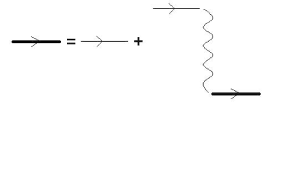
Figure 1: The graphic equation for Green’s function $\Lambda_{0\sigma}(i\omega_{p},{\textit{{q}}})$ in approximation Hubbard-I.

The solution of graphic equation in Fig.1 is

$$\beta{\kern 1.0pt}\Lambda_{0\sigma}(i\omega_{p},\textbf{q})=\frac{\beta{\kern 1.0pt}\tilde{G}_{0\sigma}(i\omega_{p})<F^{\sigma 0}>}{1-\beta t(\textbf{q})\tilde{G}_{0\sigma}(i\omega_{p})<F^{\sigma 0}>}$$ (14)

The retarded Green’s functions are obtained by the analytic continuation $i\omega_{n}\to\Omega+i\delta$ in (14) that gives a full information about electron dynamics within the framework of the approximation Hubbard-I. For simplicity we assume that T = 0. By introducing the symbol $w=(\Omega+\tilde{\mu})/\omega_{0}$ we have for unperturbed Green’s function (12)

$$\beta\tilde{G}_{0\sigma}(w\omega_{0}-\tilde{\mu})=\frac{1}{{w\omega_{0}}}(M(1,1+w,-\lambda^{2})\theta(\tilde{\mu})\kern 30.0pt$$

$$+M(1,1-w,-\lambda^{2})\theta(-\tilde{\mu})),\kern 20.0pt$$ (15)

where M(a,b,z) and $\theta(x)$ are the confluent hypergeometric function of Kummer 20 and Heaviside step function, respectively.

It is easy to find the pole singularities based on Eq.(14) that gives the spectrum of electron-hole excitation in approximation Hubbard-I:

$$\begin{array}[]{l}\varepsilon_{c.m}=4\left({\frac{{t(\textbf{k})}}{W}}\right)_{c.m}=\frac{{4(\Omega_{\textbf{k}m}+\tilde{\mu})}}{{<F^{\sigma 0}>M\left({1,1+\frac{{\Omega_{\textbf{k}m}+\tilde{\mu}}}{{\omega_{0}}},-\lambda^{2}}\right)}}\\ =-(\cos(k_{x}a)+\cos(k_{x}a)+2\alpha\cos(k_{x}a)\cos(k_{x}a)),\end{array}$$ (18)

where bandwidth W=8t$>$0. Index m enumerates the modes which are the solutions of Eq.(18). Let W=1, i.e. the frequencies, chemical potential and all energy parameters are measured in the units of bandwidth.

In Fig.2 the k dependence of resonance frequency $\Omega_{{\it k}}$ is presented. The curves were calculated along nodal direction $k_{x}$= $k_{y}$=$k/\sqrt{2}$ at a$=$3.814 $\mathop{\rm A}\limits^{o}$ at different electron concentrations and electron-phonon coupling for bismuth cuprate 2212 with phonon frequency $\omega_{0}$= 0.01875. From figure it easy to see that the inclusion of the electron-phonon coupling (g$\neq$0) results in the appearance of polaron bands the bandwidth of which is increasing with increasing g. It follows from Eq. (18) that kinks on curve $\Omega_{{\it k}}$ versus k are determined by zeros of function $M\left(1,1+\frac{\Omega_{{\it k}{\it m}}+\tilde{\mu}}{\omega_{0}},-\lambda^{2}\right)$. Computing the real zeros of hypergeometric functions is a complicated mathematical problem which can be solved only numerically 21 . However, one can state that the centre of the envelope curve of polaron bands and their total bandwidth are determined approximately by parameter $\lambda^{2}$ which counts the number of phonon quanta in the phonon cloud around the localized electron 1 , i.e. at $\frac{\Omega_{{\it k}{\it m}}+\tilde{\mu}}{\omega_{0}}\sim-\lambda^{2}$. For high electron energies the polaron band is localized and its energy is equal to energy of phonon quanta in this area of frequencies.

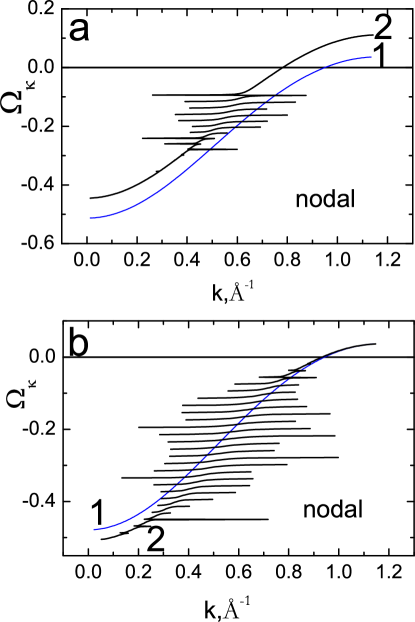
Figure 2: The electron excitation frequency-momentum dispersion along the nodal direction $k_{x}=k_{y}=k/$$\sqrt{2}$ at a$=$3.814 $\mathop{\rm A}\limits^{o}$ for bismuth cuprate 2212 with phonon frequency $\omega_{0}$= 0.01875 and a) n=0.9, $\alpha$=0.1, g=0, $\tilde{\mu}$=0.136 and g=0.03, $\tilde{\mu}$=0.092 (curves 1 and 2, respectively); b) n=0.97, $\alpha$=0.1, g=0, $\tilde{\mu}$= 0.195 and g=0.06, $\tilde{\mu}$=0.0188 (curves 1 and 2, respectively). The bandwidth W=1 hereinafter.

Let us consider the case when polarons are absent, i.e. at $\lambda=0$. Then $M\left(1,1+\frac{\Omega_{{\it k}{\it m}}+\tilde{\mu}}{\omega_{0}},-\lambda^{2}\right)$=1 and electron excitation spectrum consists from one mode and has the form:

$$\begin{array}[]{l}\Omega_{k}+\tilde{\mu}=\frac{{-1}}{4}<F^{\sigma 0}>\\ \times\left({\cos(k_{x}a)+\cos(k_{x}a)+2\alpha\cos(k_{x}a)\cos(k_{x}a)}\right)\\ \end{array}$$ (19)

The spectrum (19) has a characteristic feature which radically differentiates the metal state from state of doped Mott’s dielectrics. Indeed, the site probability ${<F^{\sigma 0}>}$ of the electron-hole state enters in Eq.(19). In general case of ordered spins $<{F^{\sigma 0}>}={1-n/2+\sigma<S^{z}}>$. In ferromagnetic phase a mean spin $<S^{z}>=n/2$ that gives $<F^{+0}>=1$ and $<F^{-0}>=1-n$. Thus, in the limit of half filled band at $n\to 1$ we have practically one band in accordance with Eq.(19). It is typical for metal state. On the other hand, in PM state $<S^{z}>=0$, $<F^{+0}>=<F^{-0}>=1-n/2$, i.e. mode (19) is two-fold degenerate. This is because in this case spin-up and spin-down electron liquids coexist in cuprates. These liquids do not interact because their Hamiltonians (11) commute. Apparently, the Fermi level must be shifted essentially since the electron liquids are in thermodynamic equilibrium. This factor should be taken into account especially when the methods of metal theory are applied to hole doped Hubbard’s systems. Let us dwell on this problem in detail by the example of calculation of chemical potential value.

To solve problem it is necessary to find the electron density of state which is determined by imaginary part of the lattice Green’s function analytically continuated to the lower half-plane 22 :

$$G(s,\alpha)\kern 100.0pt$$

$$=\frac{1}{N}\sum\limits_{\textbf{k}}{\frac{1}{{s-i\delta-cos(k_{x}a)-(1+2\alpha cos(k_{x}a))cos(k_{y}a)}}}$$

(20)

The given sum is calculated exactly. Taking into account that 2$\alpha$$<$1 one can write the real and imaginary parts of $G(s,\alpha)$ for s$>$0:

$$ReG(s,\alpha)=\left\{\begin{array}[]{l}{\frac{2}{\left|s+2\alpha\right|}\frac{1}{\pi}K\left(\frac{2\sqrt{2\alpha s+1}}{\left|s+2\alpha\right|}\right),\quad 2\alpha s+1>0,\,s>0,\;s>2(\alpha+1)}\\ {\frac{1}{\sqrt{2\alpha s+1}}\frac{1}{\pi}K\left(\frac{\left|s+2\alpha\right|}{2\sqrt{2\alpha s+1}}\right),\quad 2\alpha s+1>0,s>0,\,\,2(\alpha-1)\;\leq s\leq 2(\alpha+1)}\\ {\frac{2}{\sqrt{(2\alpha-s)^{2}-4}}\frac{1}{\pi}K\left(2\sqrt{\frac{-2\alpha s-1}{(2\alpha-s)^{2}-4}}\right),\quad 2\alpha s+1\leq 0,\,s>0,\;s>2(\alpha+1)}\end{array}\right.$$ (24)

$$ImG(s,\alpha)=\left\{\begin{array}[]{l}{\frac{1}{\sqrt{2\alpha s+1}}\frac{1}{\pi}K\left(\frac{1}{2}\sqrt{\frac{4-(2\alpha-s)^{2}}{2\alpha s+1}}\right),\quad\;2(\alpha-1)\;<s<2(\alpha+1)}\\ {0,\quad otherwise}\end{array}\right.,$$ (27)

where K(k) is a complete elliptic integral of the first order. We point out that G(s,$\alpha$) has a such symmetric property:

$$G(-s+i\delta,\alpha)=-G(s-i\delta,-\alpha)$$ (28)

Using Eq.(28) we write the next symmetric property for real part of lattice Green’s function:

$$ReG(s,-\alpha)=-ReG(-s,\alpha)$$ (29)

The pointed property allows to consider an electron spectrum type of Eq.(19) since a determination of the lattice Green’s function corresponds to hole spectrum for $s>0$. In what follows for calculations we use the left part of Eq.(29) and keep in mind that values -$\alpha$ and $\alpha$ correspond to electrons and holes, respectively. Hence, in expressions for lattice Green’s functions in the electron spectrum with parameter $\alpha$ we will take $ReG(s,-\alpha)$.

The imaginary part required for further calculations is only determined by analytic continuation in a lower half-plane independently of replacement $s\to-s$. As a result we have the next relationship for imaginary part of $G(s,\alpha)$:

$$ImG(-s,\alpha)=ImG(s,-\alpha)$$ (30)

Eqs.(29) and (30) allow to find the real and imaginary parts of $G(s,\alpha)$ for all values of s.

In Fig.3 the dependences on parameter s for real (a) and imaginary (b) parts of the lattice Green’s function (20) at $\alpha$=0, -0.4 and 0.4 (curves 1-3, respectively) are presented. From figure one can see the asymmetry of curves and van Hove singularities for nonzero values of parameter $\alpha$ that is typically for two-dimensional systems. For s=0 $ReG(s,\alpha)$ has discontinuity. It has to give rise to qualitative changing in the spectrum near the point s=0.

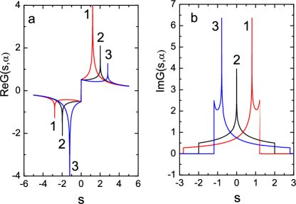
Figure 3: The s-dependences of real (a) and imaginary (b) parts of the lattice Green’s function (20) at $\alpha$=0, -0.4 and 0.4 (curves 1-3, respectively).

From Eq.(24) it follows that for transition from hole to electron consideration the sign of a resonance frequency is changed on opposite. The equation for chemical potential is determined by $ImG(s,\alpha)$ which does not depend on hole or electron formalism. One can make the summation over all wave vectors for any function V($\varepsilon$) by the use of a lattice Green’s function. Indeed, we have

$$S(\alpha)=\frac{1}{N}\sum\limits_{\textbf{q}}{V(cos(k_{x}a)+(1+2\alpha cos(k_{x}a))cos(k_{y}a))}$$

$$=\frac{1}{N}\sum\limits_{\textbf{q}}{\int\limits_{-2+2\alpha}^{2+2\alpha}{\delta(-\varepsilon-cos(k_{x}a)-(1+2\alpha cos(k_{x}a))}}$$

$$\times cos(k_{y}a))V(-\varepsilon)d\varepsilon=\int\limits_{-2-2\alpha}^{2-2\alpha}{D_{C}(\varepsilon,\alpha)V(\varepsilon)d\varepsilon},$$

where $\delta$(x) is the Dirac delta function. The electron density of state $D_{C}(\varepsilon,\alpha)$ has the form:

$$D_{C}(\varepsilon,\alpha)\kern 200.0pt$$

$$=\frac{1}{N}\sum\limits_{\textbf{q}}{\delta(\varepsilon-cos(q_{x}a)-(1+2\alpha cos(q_{x}a))cos(q_{y}a))}$$

$$=\frac{1}{\pi}{\mathop{\rm Im}\nolimits}G(\varepsilon,\alpha)\kern 100.0pt$$ (31)

Apparently, $D_{C}(\varepsilon,\alpha)$ has nonzero values for $\varepsilon$ in area from -2-2$\alpha$ to 2-2$\alpha$.

From Eq.(14) for Green’s function $\beta{\kern 1.0pt}\Lambda_{0\sigma}(i\omega_{n},\textbf{q})$ in approximation Hubbard-I we find the spectral density of the fermion-bosonic system:

$$A_{Hubb.}(\Omega,{\textbf{k}})=-2\beta Im\Lambda_{0\sigma}(\Omega+i\delta,{\textbf{k}})$$ (32)

Expanding the denominator of $\Lambda_{0\sigma}(\Omega+i\delta,{\textbf{k}})$ in a series in the vicinity of its m-th pole $E_{n{\textbf{k}}\sigma}$ we have

$$A_{Hubb.}(\Omega,{\it\textbf{k}})=-2\pi\sum_{m}\frac{\beta\tilde{G}_{0\sigma}(E_{{\it m\textbf{k}}\sigma})}{t({\textbf{k}})\frac{d\beta\tilde{G}_{0\sigma}(\Omega)}{d\Omega}}\delta(\Omega-E_{{\it m\textbf{k}}\sigma})$$ (33)

Here, the sum is over m-th modes $E_{m{\textbf{k}}\sigma}$that are the implicit solutions of dispersion Eq. (18). It is evident from Eq.(33) that approximation Hubbard-I describes coherent excitation only. Having calculated spectral density it is easy to find the equation for chemical potential. Indeed, a mean site occupancy $<X^{\sigma{\kern 1.0pt}\sigma}>$ of electron with spin $\sigma$ is determined by $A_{Hubb.}(\Omega,{\textbf{k}})$:

$$<X^{\sigma{\kern 1.0pt}\sigma}>=\frac{1}{N}\sum_{{\textbf{q}}}\frac{1}{2\pi}\int_{-\infty}^{+\infty}f(\Omega)A_{Hubb.}(\Omega,{\textbf{q}})d\Omega$$ (34)

In work 15 the method of inverse function was suggested to compute the integrals like that in Eq.(34) when an infinite number of modes $E_{n{\textbf{k}}\sigma}$ cannot be expressed as explicit. For that let us introduce the notation $\beta\tilde{G}_{0\sigma}(\Omega)=F(\Omega)$. The complicated delta function from Eq.(33) is simplified by relationship 19 :

$$W\delta[\Omega-E_{{\it m}{\textbf{q}}\sigma}]=\frac{\delta(\varepsilon-\varepsilon_{c.m})}{\left|(\Omega-E_{{\it m\textbf{q}}\sigma})^{{}^{\prime}}\right|_{\varepsilon_{c.m}}},$$ (35)

where $\varepsilon_{c.m}=\frac{4}{F(\Omega)<F^{\sigma 0}>}$ and index m gives the range $m{\kern 1.0pt}{\kern 1.0pt}\omega_{0}<\Omega<(m+1){\kern 1.0pt}{\kern 1.0pt}\omega_{0}$ in which the inverse function $F^{-1}\left(\varepsilon\right)$ is determined. Apparently, that $E_{nq\sigma}(\varepsilon)=F^{-1}\left({\frac{4}{{\varepsilon<F^{\sigma 0}>}}}\right)$ and $E_{nq\sigma}(\varepsilon_{c.m})=\Omega$. Taking into account a differentiation of the inverse function $F^{-1}\left(\varepsilon\right)$ we have

$$\left|(\tilde{\Omega}-\tilde{E}_{{\it m}{\textbf{q}}\sigma}(\varepsilon))^{{}^{\prime}}\right|_{\varepsilon=\varepsilon_{c.{\it m}}}=\left.\frac{4}{\varepsilon^{2}<F^{\sigma 0}>\left|F^{{}^{\prime}}(\varepsilon)\right|}\right|_{\varepsilon=\varepsilon_{c.{\it m}}}$$ (36)

Substituting (36) in (35) and (35) in (34) with account for $\left|F^{\prime}(\Omega)\right|/F^{\prime}(\Omega)=-1$ we obtain

$$\begin{array}[]{l}<X^{\sigma{\kern 1.0pt}\sigma}>=\sum\limits_{m=0}^{\infty}{\int\limits_{m{\kern 1.0pt}\omega_{0}}^{(m+1)\omega_{0}}{d\Omega f(\Omega)\int\limits_{-2-2\alpha}^{2-2\alpha}{d\varepsilon{\kern 1.0pt}\varepsilon D_{c}(\varepsilon,\alpha)}}}\\ \times\;\delta(\varepsilon-\varepsilon_{c.m})F(\Omega)<F^{\sigma 0}>,\end{array}$$

that gives the next expression for mean site occupancy with electron-phonon binding:

$$<X^{\sigma{\kern 1.0pt}\sigma}>=4\int_{-\infty}^{+\infty}d\Omega{\kern 1.0pt}f(\Omega)D_{c}\left(\frac{4}{F(\Omega)<F^{\sigma 0}>},\alpha\right)$$ (37)

At temperature T=0 in PM phase $<X^{\sigma{\kern 1.0pt}\sigma}>=n/2$ and from Eq.(37) we obtain the equation for chemical potential $\tilde{\mu}$:

$$\frac{n}{2}=4{\kern 1.0pt}{\kern 1.0pt}\omega_{0}\kern 150.0pt$$

$$\times\int\limits_{-\infty}^{\tilde{\mu}/\omega_{0}}{dw{\kern 1.0pt}D_{c}\left({\frac{{4w{\kern 1.0pt}{\kern 1.0pt}\omega_{0}}}{{M(1,1+w,-\lambda^{2})\left({1-0.5n}\right)}},\alpha}\right)}$$ (38)

From (38) it follows that in the absence of electron-phonon interaction the chemical potential is expressed in form 15 :

$$\tilde{\mu}=\frac{2-n}{8}I^{-1}\left(\frac{n}{2-n},\alpha\right),$$ (39)

where $I^{-1}\left(x,\alpha\right)$ is the inverse function of function $I(x,\alpha)=\int_{-2-2\alpha}^{x}D_{C}(\varepsilon,\alpha)d\varepsilon$. In particular, we have $I^{-1}\left(1,\alpha\right)=2-2{\kern 1.0pt}{\kern 1.0pt}\alpha$ and $\tilde{\mu}=\frac{1}{4}(1-\alpha)$ for n=1. Thus, in PM phase the level of chemical potential tends to the middle of upper half of a nearly half-filled band but not to band edge as it is required for normal metal. This correlation effect narrows the lower Hubbard’s band by reason of existence of two spin-up and spin-down electron liquids which are avoiding one another. For the first time this phenomena was observed by W.F. Brinkman and T.M.Rice 13 .

In Fig.4 the concentration dependencies of the effective chemical potential $\tilde{\mu}$ evaluated from Eq.(38) at g=0 for different values of $\alpha$ (a), at $\alpha$=0 for different values of g (b) and the phase diagram in coordinate g-n for $\alpha$=0 and 0.1 (curves 1 and 2,respectively) are presented. From Fig.4 a it easy to see that for n$>$0.87 the chemical potential is increased with decrease the value of $\alpha$. For n$<$0.87 in area of positive $\tilde{\mu}$ the inverse trend is observed. From Fig.4 b one sees that with increasing g the area of existence PM phase narrows and for g=0.072 a dielectric state is realized (see Fig.4 c). Thus, the effective chemical potential $\tilde{\mu}$ is decreased up to zero with increasing g, i.e. Fermi level is shifted to band centre.

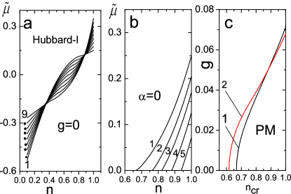
Figure 4: The concentration dependences of the effective chemical potential $\tilde{\mu}$ in approximation Hubbard-I without and with account for polaron excitations for $\omega_{0}$= 0.01875 at a) g=0 and $\alpha$=0.4, 0.3, 0.2, 0.1,0, -0.1, -0.2, -0.3 -0.4 (curves 1-9, respectively); b) $\alpha$=0 and g=0, 0.03, 0.04, 0.05 0.06 (curves 1-5, respectively); ) phase diagrams for $\alpha$=0 and 0.1 (curves 1 and 2, respectively).

In Fig.5 the critical values of -$\epsilon_{cr.}$ from Eq.(18) versus n on Fermi level when $\Omega_{{\it k}{\it m}}=0$ at g=0.03, 0.05 and 0.06 are shown. One sees that near the PM phase boundary when $\tilde{\mu}\sim 0$ the antibonding orbitals of second- nearest neighbors become important. That’s why in this area of electron concentration the Fermi surface has a hole origin with the centre in $\Gamma$ point (see Fig.6). As n is increased the electron Fermi surface is arisen. Fig.6 reflects the topology dependence of the electron Fermi surface on both electron-phonon binding and doping. One shrink as doping is decreased. With increase the constant of an electron-phonon interaction g this shrink is decreased. Also, when the hole doping goes to zero the Fermi surface does not vanish. Hence, the transition to dielectric state implies discontinuous disappearance of the Fermi surface.

Figure 5: The critical values of -$\epsilon_{cr.}$ versus n from Eq.(18) on the Fermi level at $\alpha$=0.1, g=0.03, 0.05 and 0.06 (curves 1-3, respectively).

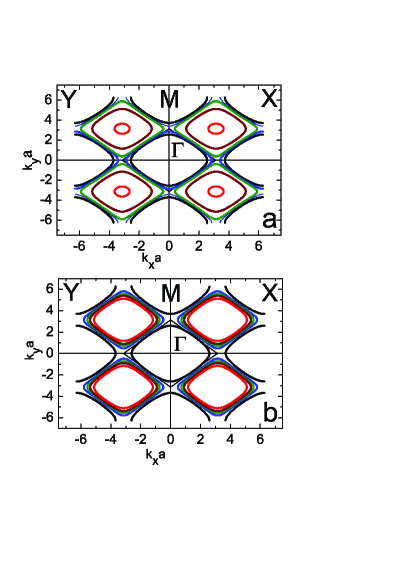
Figure 6: The Fermi surfaces in approximation Hubbard-I square of which is decreased with increase an electron concentration n at $\alpha$=0.1 and a) g= 0.03 n=0.727, 0.74, 0.76, 0.85 and 0.99 ($\tilde{\mu}$=0, 0.004, 0.011, 0.057 and 0.171, respectively); b) g=0.06 and n=0.95, 0.96, 0.97, 0.98 0.999 ($\tilde{\mu}$= 0.0004, 0.0095, 0.0188, 0.0285 and 0.0478, respectively).

III Effects of d-electron inelastic scattering

III.1 Green’s function and self-energy

In the previous section a detailed consideration of the approximation Hubbard-I was given. Although this approach does not describe an electron scattering it may be a good start to account for correlation effects.

To find the time-ordered Green’s function we will consider the contributions of the one-loop diagrams only. It is the first nonvanishing approximation of time-dependent perturbation theory with respect to the inverse effective radius of interaction. Since the phonon and fermion subsystem are independent, we have

$$\begin{array}[]{l}\Lambda_{0\sigma}(p\tau_{l},q\tau_{m})=-<T_{\tau}\tilde{X}_{p}^{0\sigma}(\tau_{p})\tilde{X}_{q}^{\sigma 0}(\tau_{q})>\\ =-U_{ep}(\tau_{p}-\tau_{q})<T_{\tau}X_{p}^{0\sigma}(\tau_{p})X_{q}^{\sigma 0}(\tau_{q})>\\ \end{array}$$

where the first factor $U_{ep}{\rm(}\tau_{p}-\tau_{q}{\rm)}{\rm}$ = ${<T}_{\tau}Y_{p}(\tau_{p})Y_{q}^{+}(\tau_{q})>_{\hat{\tilde{H}}_{b}}$ is the unperturbed time-ordered uniform bosonic Green’s function for the system of Einstein phonons. Fourier transform of $U_{ep}{\rm(}\tau_{p}-\tau_{q}{\rm)}$ is

$$U_{ep}(i\omega_{n})=\frac{1}{\beta}\sum_{m=-\infty}^{+\infty}\frac{\psi_{m}}{i\omega_{n}+m\omega_{0}},$$ (40)

where $\psi_{m}=2d_{m}\sinh\left(\beta m\omega_{0}/2\right)$, $\omega_{n}=2n{\kern 1.0pt}{\kern 1.0pt}\pi/{\kern 1.0pt}\beta$, $d_{m}=e^{-\lambda^{2}(2B+1)}I_{m}\left(2\lambda^{2}\sqrt{B(B+1)}\right)$. ${I_{m}(x)}$ are the Bessel functions of complex argument, ${\it B=n(}\omega_{0}{\it)}$. ${\it n(x)=1/(exp(}\beta{\it x)-1)}$ is Bose distribution. In the second factor the external Hubbard’s operators are not multiplied by bosonic operators $Y_{p}(\tau_{p})$ but inner ones are unitary transformed. That’s why at first the normalized Green’s function is conveniently considered in form

$$H_{0\sigma}(p\tau_{{\rm l}},q\tau_{{\rm m}}){\rm=}\frac{\Lambda_{0\sigma}(p\tau_{{\rm l}},q\tau_{{\rm m}})}{U_{ep}{\rm(}\tau_{p}-\tau_{q}{\rm)}}$$ (41)

By $\Sigma_{\sigma}({\it i}{\kern 1.0pt}{\kern 1.0pt}\omega_{n})$ denote a self-energy part of the total Green’s function $\Lambda_{0\sigma}(i\omega_{n},{\bf k})$. Then one can write the Dyson’s equation for $\Lambda_{0\sigma}(i\omega_{n},{\bf k})$ in the next form:

$$\Lambda_{0\sigma}(i\omega_{n},{\textbf{k}})=\Sigma_{\sigma}({\it i}{\kern 1.0pt}{\kern 1.0pt}\omega_{n})+\beta t({\textbf{k}})\Sigma_{\sigma}({\it i}{\kern 1.0pt}{\kern 1.0pt}\omega_{n})\Lambda_{0\sigma}(i\omega_{n},{\textbf{k}})$$

Apparently, the self-energy is expressed as

$$\Sigma_{\sigma}({\it i}{\kern 1.0pt}{\kern 1.0pt}\omega_{n})=\sum_{\omega_{n1}}U_{ep}(i\omega_{n}-i\omega_{n_{1}})H_{0\sigma}(i\omega_{n_{1}}),$$ (42)

where $H_{0\sigma}(i\omega_{n_{1}})$ is the Fourier transform of function $H_{0\sigma}(p\tau_{{\rm l}},q\tau_{{\rm m}})$. The poles is supposed to be known. Then it easy to evaluate frequency summation in Eq.(42) that gives

$$\Sigma_{\sigma}({\it i}{\kern 1.0pt}{\kern 1.0pt}\omega_{n})=\beta Res\left[f(\omega){\rm G}_{ph.}{\rm(}i\omega_{n}{\rm-}\omega{\rm)}H_{0\sigma}(\omega)\right]_{{\rm G}_{ph.}}$$

$$+\beta Res\left[f(\omega){\rm G}_{ph.}{\rm(}i\omega_{n}{\rm-}\omega{\rm)}H_{0\sigma}(\omega)\right]_{H_{0\sigma}},$$ (43)

where the residues are taken in poles of the corresponding Green’s functions.

We use the effective self-consistent field in the approximation Hubbard-I as a start. In this case account must be taken over all the inner convolutions of adjacent unitary transformed Hubbard’s operators. For dressed line of hopping integral $B_{\sigma 0}(\tau_{j}-\tau_{i},{\textbf{R}}_{j}-{\textbf{R}}_{i})$ with Fourier transform $B_{\sigma 0}(i{\kern 1.0pt}{\kern 1.0pt}\omega_{n},{\textbf{k}})$ one can write the graphic equation in form as in Fig.7. Here, the thin and bold wave lines are $\beta t({\textbf{k}})$ and $\beta B_{\sigma 0}(i{\kern 1.0pt}{\kern 1.0pt}\omega_{n},{\textbf{k}})$, respectively. The thin straight arrow corresponds to $\tilde{G}_{0\sigma}(i\omega_{n})<F^{\sigma 0}>$ from Eq.(12).

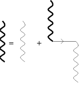
Figure 7: Graphic equation for the effective hopping integral $B_{\sigma 0}(i{\kern 1.0pt}{\kern 1.0pt}\omega_{n},{\it k})$.

The solution of this equation is trivial and has a form:

$$\beta B_{\sigma 0}(i{\kern 1.0pt}{\kern 1.0pt}\omega_{n},{\textbf{k}})=\frac{\beta t({\textbf{k}})}{1-\beta t({\textbf{k}})\tilde{G}_{0\sigma}(i\omega_{n})<F^{\sigma 0}>}$$ (44)

Then in this approach two main terms must be added to unperturbed Green’s function $G_{0+}(\tau_{p}-\tau_{q})<F^{+0}>_{0}$:

$$\begin{array}[]{l}\int\limits_{0}^{\beta}{d\tau_{1}\int\limits_{0}^{\beta}{d\tau_{2}\frac{1}{N}\sum\limits_{ij\textbf{q}}{\frac{1}{\beta}B_{+0}(\tau_{1}-\tau_{2},\textbf{q})e^{i\textbf{q}(\textbf{R}_{l}-\textbf{R}_{m})}}}}\times\\ <T_{\tau}X_{p}^{0+}(\tau_{p})X_{q}^{+0}(\tau_{q})Y_{l}^{+}(\tau_{1})X_{l}^{+0}(\tau_{1})Y_{m}(\tau_{2})X_{m}^{0+}(\tau_{2})>_{0}\end{array}$$

and

$$\begin{array}[]{l}\int\limits_{0}^{\beta}{d\tau_{1}\int\limits_{0}^{\beta}{d\tau_{2}\frac{1}{N}\sum\limits_{ij\textbf{q}}{\frac{1}{\beta}B_{-0}(\tau_{1}-\tau_{2},\textbf{q})e^{i\textbf{q}(\textbf{R}_{l}-\textbf{R}_{m})}}}}\times\\ <T_{\tau}X_{p}^{0+}(\tau_{p})X_{q}^{+0}(\tau_{q})Y_{l}^{+}(\tau_{1})X_{l}^{-0}(\tau_{1})Y_{m}(\tau_{2})X_{m}^{0-}(\tau_{2})>_{0}\\ \end{array}$$

Using the Vick’s theorem for Hubbard’s operators and taking into account an independent averaging of a product of the bosonic operators $Y_{m}(\tau_{2})$ we evaluate these integrals. In Fig.8 the self-energy terms in form to linked diagrams ( points in Fig.8 denote index convolutions) are presented generally for $\sigma$=$\pm$ . In figure the dash line with arrow corresponds to bosonic unperturbed Green’s function $G_{+-}(i\omega_{n})=1/(\beta(i\omega_{n}+\varepsilon_{+}-\varepsilon_{-}))$ where $\varepsilon_{+}-\varepsilon_{-}=-h$ and h is the effective exchange field.

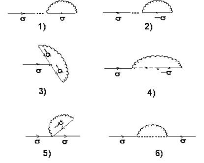
Figure 8: Diagrams for the self-energy $\Sigma_{\sigma}({\it i}{\kern 1.0pt}{\kern 1.0pt}\omega_{n})$ in the first approximation of the perturbation theory 14 .

Let us write the analytic expressions for diagrams 1-3:

$$\begin{array}[]{l}{\rm 1)}-\beta\delta\tilde{\mu}_{\sigma}\partial_{\sigma}<F^{\sigma 0}>_{0}G_{0\sigma}(i\omega_{n})=-\frac{1}{N}\sum\limits_{\textbf{q}n_{1}}{{\kern 1.0pt}\beta}\\ \times\tilde{G}_{0\sigma}(i\omega_{n_{1}})B_{\sigma 0}(i\omega_{n_{1}},{\bf q})\partial_{\sigma}<F^{\sigma 0}>_{0}G_{0\sigma}(i\omega_{n})\\ 2)-\beta\delta\tilde{\mu}_{-\sigma}\partial_{-\sigma}<F^{\sigma 0}>_{0}G_{0\sigma}(i\omega_{n})=-\frac{1}{N}\sum\limits_{\textbf{q}n_{1}}{{\kern 1.0pt}\beta}\\ \times\tilde{G}_{0-\sigma}(i\omega_{n_{1}})B_{-\sigma 0}(i\omega_{n_{1}},{\bf q})\partial_{-\sigma}<F^{\sigma 0}>_{0}G_{0\sigma}(i\omega_{n})\\ 3)\;\tilde{\nu}_{-\sigma}<F^{-\sigma 0}>_{0}G_{0\sigma}(i\omega_{n})\,=\frac{1}{N}\sum\limits_{\textbf{q}n_{1}m_{1}}{B_{-\sigma 0}(i\omega_{n_{1}},{\bf q}){\kern 1.0pt}}\\ \times U_{ep}(i\omega_{n_{1}}-i\omega_{m_{1}})\left[{G_{0-\sigma}(i\omega_{m_{1}})}\right]^{2}<F^{\sigma 0}>_{0}\beta G_{0\sigma}(i\omega_{n})\\ \end{array}$$

Here, the derivative $\partial_{\sigma}<F^{\sigma 0}>_{0}=\partial<F^{\sigma 0}>_{0}/\partial(-\beta{\kern 1.0pt}\varepsilon_{\sigma})$ and ${\kern 1.0pt}\varepsilon_{\sigma}=-\tilde{\mu}$. These diagrams are proportional to external unperturbed Green’s function $G_{0\sigma}(i\omega_{n})=1/(\beta(i\omega_{n}+\tilde{\mu}))$. One can factor out and add $G_{0\sigma}(i{\kern 1.0pt}{\kern 1.0pt}\omega)<F^{+0}>_{0}$. Then in parentheses we obtain a series expansion for an average $<F^{\sigma 0}>=1-n/2$. This series was considered in work [15]. It gives an equation for chemical potential $\tilde{\mu}$. Therefore, the sum of diagram terms 1-3 and $G_{0\sigma}(i{\kern 1.0pt}{\kern 1.0pt}\omega)<F^{+0}>_{0}$ gives a contribution $G_{0\sigma}(i{\kern 1.0pt}{\kern 1.0pt}\omega_{n})(1-n/2)$ to $H_{0\sigma}(i\omega_{n_{1}})$.

The contribution from diagram 5 to $H_{0\sigma}(i\omega_{n_{1}})$ is written as 5) $-\beta\delta\tilde{\mu}_{-\sigma}<F^{\sigma 0}>_{0}G_{0\sigma}^{2}(i\omega_{n})$ One can prove that diagrams 4 and 6 only differs by factors $<X^{\sigma\sigma}>_{0}$ and $<F^{\sigma 0}>_{0}/(1-<F^{\sigma 0}>_{0})$, respectively, i.e. one writes

$$\begin{array}[]{l}4)+6)=K_{0}(I_{1}(i\omega_{n})+I_{2}(i\omega_{n}))G_{0\sigma}^{2}(i{\kern 1.0pt}{\kern 1.0pt}\omega_{n}),\end{array}$$

where $K_{0}=<X^{\sigma\,\sigma}>_{0}+<F^{\sigma 0}>_{0}(1-<F^{\sigma 0}>_{0})$=3/4 at T=0. Evaluating the sum over inner discrete frequencies by means of previously considered method of inverse function we write the final expression for $H_{0\sigma}(i\omega_{n})$:

$$H_{0\sigma}(i\omega_{n})=G_{0\sigma}(i{\kern 1.0pt}{\kern 1.0pt}\omega_{n})(1-n/2)+K_{0}(I_{1}(i\omega_{n})$$

$$+I_{2}(i\omega_{n}))G_{0\sigma}^{2}(i{\kern 1.0pt}{\kern 1.0pt}\omega_{n})-\beta\delta\tilde{\mu}_{-\sigma}<F^{\sigma 0}>_{0}G_{0\sigma}^{2}(i\omega_{n}),$$ (45)

$$\begin{array}[]{l}{I_{1}(i\omega_{n})=\int_{-\infty}^{+\infty}d\Omega\frac{4\beta f(\Omega)\tilde{D}_{C}\left({\Omega,\ \ \alpha}\ \right)}{\left[F(\Omega)<F^{\sigma 0}>\right]^{2}}\beta U_{ep}(\Omega-i\omega_{n}){\kern 1.0pt}}\\ \\ {I_{2}(i\omega_{n})=\frac{1}{N}\sum\limits_{{\textbf{q}}m_{1}=-\infty}^{+\infty}\frac{\beta t({\textbf{q}})({\it n(m}_{{\it 1}}{\it\omega}_{{\it 0}}{\it)}+1)\psi_{m_{1}}}{1-t({\textbf{q}})<F^{\sigma 0}>\beta\tilde{G}_{0\sigma}(i\omega_{n}-{\it m}_{{\it 1}}{\it\omega}_{{\it 0}})}}\end{array}$$ (46)

where $\tilde{D}_{C}(\Omega,\alpha)=D_{C}\left({\frac{4}{{F(\Omega)<F^{\sigma 0}>}},\alpha}\right)$. It follows from presented above expressions that diagrams 4 and 6 describe electron-polaron and electron-electron scattering only. The rest of diagrams renormalize the excitation spectrum. At T ${\sim}$ 0 the factor $({\it n(m}_{{\it 1}}{\it\omega}_{{\it 0}}{\it)}+1)\psi_{m_{1}}$in $I_{2}(i\omega_{n})$ may be simplified. It easy to find that $\psi_{m}\approx\tilde{\psi}(\left|m\right|)sign(m)\;$, where $\tilde{\psi}(m)=e^{-\lambda^{2}}\frac{\lambda^{2m}}{m!}\;,\;sign(0)=0$ and $({\it n(m}_{{\it 1}}{\it\omega}_{{\it 0}}{\it)}+1)\psi_{m_{1}}\approx\tilde{\psi}(\left|m\right|)\theta(m)$. After analytic continuation $i{\kern 1.0pt}{\kern 1.0pt}\omega_{n}\to\omega+i\delta$ the real part of integral $I_{1}(\omega)$ is evaluated numerically as Cauchy principal value. The imaginary part of $I_{1}(\omega)$ is easy calculated since $I_{m}[\beta U_{ep}(\Omega-\omega-i\delta)]$ gives the Dirac delta function.

To obtain the final expression for self-energy $\Sigma_{\sigma}({\it i}{\kern 1.0pt}{\kern 1.0pt}\omega_{n})$ it is necessary to substitute $H_{0\sigma}(i\omega_{n})$ in Eq.(43). As result in the limit T ${\sim}$ 0 we have

$$\Sigma_{\sigma}({\it i}{\kern 1.0pt}{\kern 1.0pt}\omega_{n})=P_{0}({\it i}{\kern 1.0pt}{\kern 1.0pt}\omega_{n})+P_{5}({\it i}{\kern 1.0pt}{\kern 1.0pt}\omega_{n})+P_{46}({\it i}{\kern 1.0pt}{\kern 1.0pt}\omega_{n})$$ (47)

where

$$\begin{array}[]{l}{P_{0}(\omega)=\frac{1-0.5n}{\beta(\omega+\tilde{\mu})}M\left(1,1+\frac{\omega+\tilde{\mu}}{\omega_{0}},-\lambda^{2}\right)}\\ {P_{5}(\omega)=-<F^{\sigma 0}>_{0}\frac{1}{\beta}\delta\mu_{-\sigma}\sum\limits_{m=0}^{\infty}e^{-\lambda^{2}}\frac{\lambda^{2m}}{m!}\frac{1}{(\omega+m\omega_{0}+\tilde{\mu})^{2}}}\\ =-\frac{1}{\beta}\frac{J_{5}(\omega)}{(\omega+\tilde{\mu})^{2}}\\ {P_{46}(\omega)=J_{1}(\omega)+J_{2}(\omega)+J_{3}(\omega)}\end{array}$$ (48)

Here, ${\it w(}\omega{\it)=}\frac{\omega+\tilde{\mu}}{\omega_{0}}$ and $J_{5}(\omega)={<F^{\sigma 0}>_{0}}\delta\mu_{-\sigma}e^{-\lambda^{2}}{}_{2}F{}_{2}({\it w},{\it w};1+{\it w},1+{\it w};\lambda^{2})$, where ${}_{2}F{}_{2}({\it w},{\it w};1+{\it w},1+{\it w};\lambda^{2})$ is the generalized hypergeometric function. For T=0 we have $<F^{\sigma 0}>_{0}=1/2$ and

$$\begin{array}[]{l}J_{1}(\omega)=\sum_{m_{1},m_{2}=-\infty}^{+\infty}K_{0}\frac{1}{\beta^{2}}\frac{\psi_{m_{1}}\psi_{m_{2}}({\it n}(m_{1}\omega_{0})-{\it n}(m_{2}\omega_{0}))}{(\omega+{\it i}\delta+m_{1}\omega_{0}+\tilde{\mu})^{2}}\\ \times\int_{-\infty}^{+\infty}d\Omega\frac{{\rm Z}(\Omega,n,\alpha)f(\Omega)}{\Omega-\omega-i\delta+(m_{2}-m_{1})\omega_{0}},\kern 30.0pt\end{array}$$ (51)

where ${\rm Z}(\Omega,n,\alpha)=\tilde{D}_{C}\left(\Omega,-\alpha\right)\frac{{4\beta}}{{\left({\beta\tilde{G}_{0\sigma}(\Omega)<F^{\sigma 0}>}\right)^{2}}}$

$$J_{2}(\omega)=\sum_{m_{1},m_{2}=-\infty}^{+\infty}K_{0}\frac{1}{\beta^{2}}\frac{\psi_{m_{1}}\psi_{m_{2}}({\it n}(m_{1}\omega_{0})-n(m_{2}\omega_{0}))}{(\omega+{\it i}\delta+m_{1}\omega_{0}+\tilde{\mu})^{2}}\frac{1}{N}\sum_{{\textbf{q}}}\frac{\beta t({\textbf{q}})({\it n}(\left[m_{2}-m_{1}\right]\omega_{0})+1)}{1-t({\textbf{q}})<F^{\sigma 0}>\beta\tilde{G}_{0\sigma}(\omega+{\it i}\delta-\left[m_{2}-m_{1}\right]\omega_{0})}$$ (52)

$$J_{3}(\omega)=\sum_{m_{1},m_{2}=-\infty}^{+\infty}K_{0}\frac{1}{\beta^{2}}\frac{\psi_{m_{1}}\psi_{m_{2}}({\it n}(m_{2}\omega_{0})+f(-\tilde{\mu}))}{(\omega+{\it i}\delta+m_{1}\omega_{0}+\tilde{\mu})^{2}}\int_{-\infty}^{+\infty}d\Omega\frac{{\rm Z}(\Omega,n,\alpha)f(\Omega)}{\Omega+m_{2}\omega_{0}+\tilde{\mu}}\cdot\left(1+\frac{\omega+m_{1}\omega_{0}+\tilde{\mu}}{\Omega+m_{2}\omega_{0}+\tilde{\mu}}\right)$$ (53)

$$\delta\mu_{-\sigma}=\int_{-\infty}^{+\infty}\frac{1}{\beta}{\rm Z}(\Omega,n,\alpha)\beta\tilde{G}(\Omega)f(\Omega)$$ (54)

In Eq.(52) for ${m_{1}=m_{2}}$ the uncertainty is observed. Thus, in the limit ${m_{1}}\to{m_{2}}$ we have the function

$$J_{0}(\omega)=\frac{{K_{0}e^{-2\lambda^{2}}}}{{\beta(\omega+i\delta+\tilde{\mu})^{2}}}\kern 100.0pt$$

$$\times\frac{1}{N}\sum\limits_{\textbf{q}=-\infty}^{+\infty}{\frac{1}{{1-t(\textbf{q})<F^{\sigma 0}>\beta\tilde{G}_{0\sigma}(\omega+i\delta)}}}$$ (55)

which is determined by lattice Green’s function $G(s,\alpha)$. And so, for sum (52) the term with ${m_{1}=m_{2}}$ is excluded. It is necessary to add the expression (55) to Eq.(52) instead of this abnormal term.

One writes for imaginary part $J_{1}(\omega)$ at T=0

$$ImJ_{1}(\omega)=\frac{4\pi K_{0}}{\beta\left(1-0.5n\right)^{2}}\kern 100.0pt$$

$$\times\sum_{m=-\infty}^{\infty}R(\omega,\tilde{\mu},m)\omega_{0}^{2}\varphi\left(\frac{\omega+\tilde{\mu}}{\omega_{0}},n\right)\theta(m\omega_{0}-\omega),$$ (56)

where

$$\begin{array}[]{l}\varphi(w,n)=\tilde{D}_{C}\left(w\Omega_{0}-\mu,-\alpha\right)\frac{w^{2}}{M^{2}(1,1+w,-\lambda^{2})}\end{array}$$ (58)

$$R(\omega,\tilde{\mu},m)=\sum_{m_{1}=-\infty}^{+\infty}\frac{\left\{\tilde{\psi}(\left|m+m_{1}\right|)\tilde{\psi}(\left|m_{1}\right|)sign(m+m_{1})\theta(m_{1})-\tilde{\psi}(\left|m_{1}\right|)\tilde{\psi}(m+\left|m_{1}\right|)sign(m_{1})\theta(m+m_{1})\right\}}{(\omega+\tilde{\mu}+m_{1}\omega_{0})^{2}}$$

Notice that $R(\omega,\tilde{\mu},m)=0$ at m=0. The real part of $J_{1}(\omega)$ and complex function $J_{2}(\omega+i\delta)$ are expressed as

$$ReJ_{1}(\omega)=\frac{1}{\beta}K_{0}\sum_{m=0}^{\infty}R(\omega,\tilde{\mu},m)I_{11}(\omega,n,m)$$ (59)

$$J_{2}(\omega)=\frac{K_{0}}{\beta}\sum_{m=-\infty}^{+\infty}R(\omega,n,m)S_{2}(\omega,n,\alpha,m)$$ (60)

Here,

$$I_{11}(\omega,n,m)=\frac{{\kern 1.0pt}4\omega_{0}^{2}}{(1-0.5{\it n})^{2}}\left\{\sum_{k=-\infty}^{-1}V.p.\int_{k}^{k+1}dw\frac{\varphi(w)}{w-\left(\frac{\omega+\tilde{\mu}}{\omega_{0}}+m\right)}+V.p.\int_{0}^{\tilde{\mu}/\omega_{0}}dw\frac{\varphi(w)}{w-\left(\frac{\omega+\tilde{\mu}}{\omega_{0}}+m\right)}\right\}$$ (61)

$$S_{2}(\omega,n,\alpha,m)=\frac{\omega+\tilde{\mu}-m\omega_{0}}{\left(1-0.5n\right)M\left(1,1+\frac{\omega+\tilde{\mu}}{\omega_{0}}-m,-\lambda^{2}\right)}\left\{-1+(\omega+\tilde{\mu}-m\omega_{0})S_{3}(\omega,n,\alpha,m)\right\}$$ (62)

$$S_{3}(\omega,n,\alpha,m)=\frac{4}{\left(1-0.5n\right)M\left(1,1+\frac{\omega+\tilde{\mu}}{\omega_{0}}-m,-\lambda^{2}\right)}G^{*}\left(\frac{4\omega_{0}\left[\frac{\omega+\tilde{\mu}}{\omega_{0}}-m\right]}{(1-0.5n)M\left(1,1+\frac{\omega+\tilde{\mu}}{\omega_{0}}-m,-\lambda^{2}\right)},\alpha\right),$$ (63)

where the integrals are evaluated numerically as Cauchy principal value and integrand $\varphi(w,n)$ is determined by Eq.(58). $G^{*}(s,\alpha)$ is the conjugate lattice Green’s function.

Thus, Eqs.(47)-(63) contains a total information about spectral properties of the cuprate d-electron subsystem with electron-phonon binding. Below it is given a numerical solution of the previously obtained equations to analyze both the excitation spectrum and dissipation were caused by electron-electron and electron-polaron interactions. Finally, let us write the contribution $\textit{P}_{46}$($\omega$) in form:

$$P_{46}(\omega)=J_{0}(\omega)+J_{1}(\omega)+J_{2}(\omega)+J_{3}(\omega),$$

where $R(\omega,\tilde{\mu},m)=0$ for $\textit{m}=0$.

III.2 Electron spectrum in the absence of electron-phonon interaction

In this section we will study the dynamical properties of electrons for temperature $T$=0 in the absence of electron phonon binding, i.e. at $g$=0. Before we proceed further, we evaluate numerically the chemical potential $\tilde{\mu}$. In works 15 ; 23 it was presented an approach to calculate the chemical potential versus band filling. In particular, in 15 we obtained Eq.(51) for $\tilde{\mu}$ versus n in PM-2 state with the nearest hopping energy. One can generalize this equation when the influence of next-nearest neighbors is taken into account, i.e. for $\alpha$$\neq$0:

$$\tilde{\mu}=\frac{{2-n}}{8}I^{-1}\left({1-\frac{1}{2}(1-n)(2-n),\,{\kern 1.0pt}\alpha}\right)$$ (64)

were $I^{-1}(x,\alpha)$ is the inverse function of function $I(x,\alpha)$ (see Eq. (39)). Similarly, the term $\delta\mu_{\sigma}$ of diagram 5 in Fig.8 is

$$\delta\mu_{\sigma}=E\left(I^{-1}\left(1-\frac{1}{2}(1-n)(2-n),\,{\kern 1.0pt}\alpha\right)\right),$$ (65)

where

$$E(x,\alpha)=\int_{-2-2\alpha}^{x}{xD_{C}(x,{\kern 1.0pt}{\kern 1.0pt}{\kern 1.0pt}\alpha)dx}$$ (66)

In Fig.9 a the concentration dependencies of chemical potential at $\alpha$= -0.4, -0.3, -0.2, -0.1, 0, 0.1, 0.2, 0.3 0.4 (curves 1-9, respectively) are presented. In Fig.9 b an area of existence of the PM-2 phase in coordinates $\alpha$-n is shown. From Eq.(64) it follows that chemical potential $\tilde{\mu}$ of filled band coincides with the solution (39) in approximation Hubbard-I.

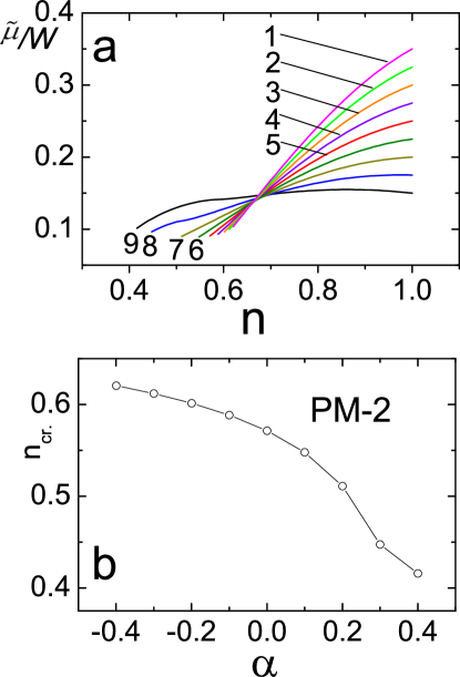
Figure 9: a) The concentration dependencies of the chemical potential in PM-2 phase with g=0 and $\alpha$= -0.4, -0.3, -0.2, -0.1, 0, 0.1, 0.2, 0.3 0.4 (curves 1-9, respectively); b) phase diagram in the $\alpha$-n plane at T=0.

The spectral density function is expressed as

$$A({\it k},\,\,\omega)=-\frac{1}{\pi}\frac{(\omega+\tilde{\mu})^{4}\beta Im\Sigma(\omega)}{\left[(\omega+\tilde{\mu})^{2}-t({\it k})(\omega+\tilde{\mu})^{2}\beta Re\Sigma(\omega)\right]^{2}+(\omega+\tilde{\mu})^{2}t^{2}({\it k})\left[(\omega+\tilde{\mu})^{2}\beta Im\Sigma(\omega)\right]^{2}}$$ (67)

In view of (43) at ${T=0}$ and ${K_{\rm 0}{\rm=3/4}}$ we have

$$\begin{array}[]{l}{(\omega+\tilde{\mu})^{2}\beta Re\Sigma(\omega)=(\omega+\tilde{\mu})\left[1-0.5n-\frac{3}{4(1-0.5n)}\right]+\frac{3(\omega+\tilde{\mu})^{2}}{(1-0.5n)^{2}}ReG\left(\frac{4(\omega+\tilde{\mu})}{1-0.5n},-\alpha\right)-0.5\,\delta\mu_{\sigma}}(\omega+\tilde{\mu})^{2}\\ \beta Im\Sigma(\omega)=-\frac{3(\omega+\tilde{\mu})^{2}}{(1-0.5n)^{2}}\pi D_{C}\left(\frac{4(\omega+\tilde{\mu})}{1-0.5n},-\alpha\right)\end{array}$$ (70)

Taking into account Eq.(70) it easy to write the dispersion equation

$$\begin{array}[]{l}-\varepsilon_{c.}(\Omega_{k})\kern 100.0pt\\ =\cos(k_{x}a)+\cos(k_{x}a)+2\alpha\cos(k_{x}a)\cos(k_{x}a)\\ =-\frac{{4(\Omega_{k}+\tilde{\mu})^{2}}}{{(\Omega_{k}+\tilde{\mu})^{2}\beta{\mathop{\rm Re}\nolimits}\Sigma(\Omega_{k})}}\end{array}$$ (74)

From Eq.(74) it is seen that now the excitation spectrum depends on real part $ReG(s,-\alpha)$ of the lattice Green’s function (24) which has both two singularities at the edges of unperturbed electron band, i.e. at ${s{\rm=}s_{\rm L}{\rm=-2(1+}\alpha{\rm)}}$ and ${s{\rm=}s_{\rm R}{\rm=2(1-}\alpha{\rm)}}$. Also, there is one breakdown at s=0 (see Fig.3 a) that corresponds to frequency ${\Omega_{{\it k}}=-\tilde{\mu}}$. These circumstances cause the cardinal changes to the spectrum of the electron excitations in comparison with approximation Hubbard-I.

In Fig. 10 the resonance frequencies $\Omega_{{\it k}}$ along the nodal direction for bismuth cuprate 2212 at different electron band filling are shown. In Fig.10 the values of n correspond to the most typical points of function $-\varepsilon_{c.}$(n) from (74) at $\Omega_{{\it k}}=0$ (Fermi level) to be shown in insert to figure. So, at $\alpha$=0 (curve 1 in insert ) the curve $-\varepsilon_{c.}$(n) tends to own lower edge -2 at n=0.7. For this value of n a small gap arises on the Fermi level. It has a correlation origin that is reflected in Fig.10 a (curve 2). A such gap (see Fig.10, curves 1 and 3) is absent at other values of n. The function $-\varepsilon_{c.}(n)$ does not approach the edge value -2-2$\alpha$ with increase an influence of the next-nearest neighbours where paramagnetic phase is realized. In this case a gap does not appear on the Fermi level for all possible values of n (see Fig. 10 b). One can point out the next main peculiarities of the spectrum in Fig.10 b. The kinks in the dispersion $\Omega_{{\it k}}$ at $\Omega_{\rm k}=\omega_{L}=-0.531$ and $\Omega_{\rm k}=\omega_{R}=0.019$ for n=0.9 (curve 3) are determined by equation

$$\frac{4(\omega+\tilde{\mu})}{1-0.5n}-s=0$$ (75)

at ${\rm}s=s_{L}$ and $s_{R}$, respectively. From this equation we obtain the lower $\omega_{L}=-\tilde{\mu}-0.5(1+\alpha)(1-0.5n)$ and upper $\omega_{L}=-\tilde{\mu}+0.5(1-\alpha)(1-0.5n)$ edges of incoherent spectrum the bandwidth $\Delta\omega_{LR}=1-0.5n$ of which is determined by electron concentration only.

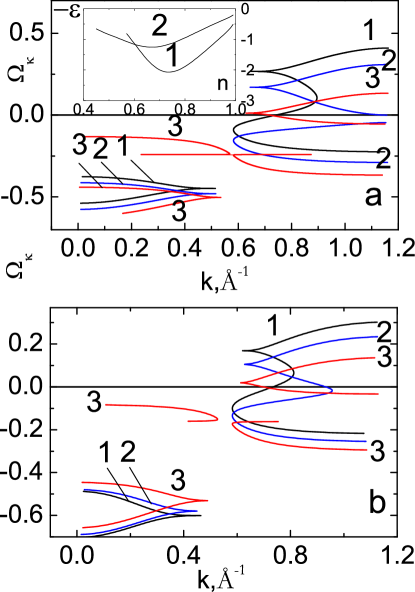
Figure 10: The electron excitation frequency-momentum dispersions for bismuth cuprate 2212 (lattice constant $a=3.814\AA$) along the nodal direction without electron-phonon binding: a) $\alpha$=0, n=0.571 ($\tilde{\mu}$=0.090), n=0.7 ($\tilde{\mu}$=0.155) and n=0.97 ($\tilde{\mu}$=0.245); b) $\alpha$=0.3, n=0.46 ($\tilde{\mu}$=0.101), n=0.63 ($\tilde{\mu}$=0.134) n=0.90 ($\tilde{\mu}$=0.173) (curves 1-3, respectively). In inset: -$\varepsilon_{c.}$ versus n on the Fermi level ($\Omega_{{\it k}}$=0) from dispersion Eq. (74) for $\alpha$=0 and $\alpha$=0.3 (curves 1 and 2, respectively).

Thus, the imaginary part of the lattice Green’s function is equal zero out of indicated area and the electron excitations are coherent. Also, two peculiarities are determined by equation (75) at s=0 and s=2$\alpha$. In this case the real and imaginary parts of $G(s,\alpha)$ have discontinuity and van Hove singularity, respectively. In excitation spectrum near the indicated points there is a sufficiently complicated dispersion with appearance of pseudogaps.

Therefore, the inclusion of the electron-electron scattering in cuprate planes causes an essential rebuilding of the excitation spectrum in comparison with approximation Hubbard-I where this scattering is absent. A correlation gap appears on the Fermi level in the area of electron concentrations when $-\varepsilon_{c.}$(0)$\leq-2+2\alpha$ that leads to disappearance of the Fermi surface.

In Fig.11 the Fermi surfaces are presented with account for electron-electron scattering in accordance with formula (74) at $\Omega_{{\it k}}=0$. The no-monotone change in Fermi surface square in Fig.11 a and b takes place in accordance with dependences $-\varepsilon_{c.}$(n) ( see curves 1 and 2 in inset to Fig. 10 a). In Fig.11 b the electron Fermi surfaces at n=0.46 and 0.63 are shown. At n=0.9 we have the hole Fermi surface.

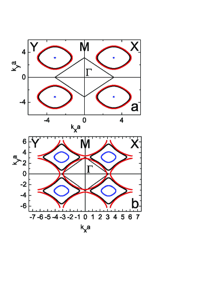
Figure 11: The electron and hole Fermi surfaces in the absence of the electron-phonon binding. The values of the parameters are as in Fig.10. In Fig. 11 a the inner surfaces as point and big oval are obtained for n=0.7 and 0.571, respectively. The outside surface corresponds to n=0.97. In Fig. 11 b the electron Fermi surfaces as deformed square and inner oval centered out of $\Gamma$ point are shown for n=0.46 and 0.63, respectively. The hole Fermi surface has a shape of the big oval centered on point $\Gamma$ at n=0.9, where $\Gamma$ is the center of Brillouin band.

It is interesting to study the corresponding spectral densities using Eq.(70). In accordance with ARPES terminology 1 let EDC denote the frequency dependence $A({\textbf{k}},\,\omega)$ along nodal direction (${k_{x}=k_{y}}$) of k at fixed value of its module. MDC spectral density is evaluated from $A({\textbf{k}},\,\omega)$ at fixed frequency along nodal direction for different values of ${k}$.

In Fig. 12 a the EDC spectral densities at $\alpha$=0 and g=0 for Fermi momentum ${k=k_{F}}$ and different electron concentration (a) and near the ${k_{F}}$ at n=0.97 (b) are shown. The EDC curves have asymmetrical character that is in accordance with experimental results 9 ; 10 . From this figure it easy to see that the maxima of $A({\textbf{k}},\,\omega)$ correspond to resonance frequencies in Fig.10 a. At the same time, the maximum at ${k=k_{F}}$ is on the Fermi level. Notice that degree of excitation coherence near the Fermi level is abruptly increased for a peculiar area of the electron spectrum where there is a frequency change from electron (${\raise 3.01385pt\hbox{$\partial\Omega_{{\it k}}$}\!\mathord{\left/{\vphantom{\partial\Omega_{{\it k}}\partial k}}\right.\kern-1.2pt}\!\lower 3.01385pt\hbox{$\partial k$}}>0$) to hole (${\raise 3.01385pt\hbox{$\partial\Omega_{{\it k}}$}\!\mathord{\left/{\vphantom{\partial\Omega_{{\it k}}\partial k}}\right.\kern-1.2pt}\!\lower 3.01385pt\hbox{$\partial k$}}<0$) character. Indeed, near the Fermi level the curve 1 in Fig.12 a is very washed out unlike the curve 3 that corresponds the curve 3 in Fig.10 a with a kink at $\Omega_{{\it k}}\sim 0$. On the other hand, the curve 2 in Fig.12 a reflects an incoherent character of the electron excitations that is in agreement with a nearly point Fermi surface in Fig. 11 a.

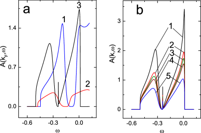
Figure 12: EDC spectral density $A({\it k},\,\,\omega)$ from Eq. (67) as a function of the frequency at $a=3.814\AA$, $\alpha$=0 and g=0 along nodal direction of the wave vector k with module a) ${k=k_{F}}$ at n=0.571, 0.7 and 0.97 (curves 1-3, respectively); b) ${{k=k_{F}}-0.05}$, ${k_{F}-0.01}$, ${k_{F}}$, ${k_{F}+0.01}$ and ${k_{F}+0.05}$, where ${k_{F}=0.717}$ at n=0.97 (curves 1-5, respectively).

In Fig.13 the MDC spectral density $A({\it k},\,\,\omega)$ versus $\left|{\it k}\right|$ along nodal direction at n =0.97 for different frequencies (a) and frequency dependence maxima of $A({\it k},\,\,\omega)$ (b) are presented. The curve $A({\it k},\,\,\omega)$ has a Lorentz line shape that is in agreement with ARPES data. Also, we observe a nontrivial character of the frequency dependence maxima of $A({\it k},\,\,\omega)$.The maximum of $A({\it k},\,\,\omega)$ appears at ${k_{max}=0.647}$ on the Fermi level when Fermi momentum is equal 0.717. Thus, the maxima of MDC spectral density do not correspond to resonance frequencies of the electron excitation spectrum.

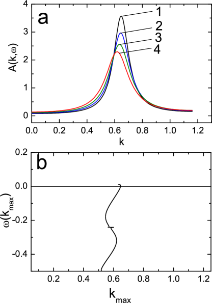
Figure 13: MDC spectral density $A({\it k},\,\,\omega)$ from Eq.(67) as function of a wave vector module at $a=3.814\AA$, n=0.97, $\alpha$=0 and g=0 along nodal direction of k: a) $\omega$= 0, -0.01, -0.025 and -0.05 (curves 1-4, respectively); b) frequency dependence of $A({\it k},\,\,\omega)$ maxima.

In Fig.14 the similar dependencies of $A({\it k},\,\,\omega)$ are shown with account for an influence the next-nearest neighbors. It was considered the electron concentration n=0.46 only when a correlation gap on the Fermi level is not developed. All conclusions to be formulated earlier in relation to Figs.12 and 13 here remain valid. Strong coherent modes appear near ${k\sim 0.6}$. It is a result of the abrupt change of derivation ${\raise 3.01385pt\hbox{$\partial\Omega_{{\it k}}$}\!\mathord{\left/{\vphantom{\partial\Omega_{{\it k}}\partial k}}\right.\kern-1.2pt}\!\lower 3.01385pt\hbox{$\partial k$}}$ (see Fig.10.b) for $\Omega_{{\it k}}=-\tilde{\mu}$. The edges of area of abrupt changing $A({\it k},\,\,\omega)$ are determined by Eq.(75) at ${\rm}s=s_{L}$ and $s_{R}$. It is noted that van Hove anomaly (see Fig.14 b at ${\omega\sim-0.1)}$ is determined by expression $\omega=\Omega_{{\it k0}}=-\tilde{\mu}+0.5\alpha(1-0.5n)$. It reflects a low-dimensional character of the electron behavior.

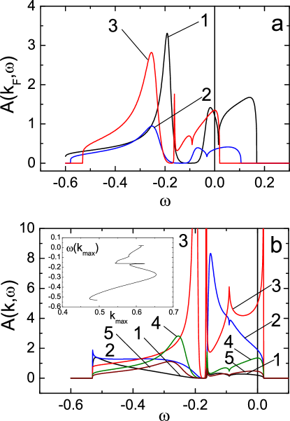
Figure 14: EDC spectral density $A({\it k},\,\,\omega)$ from Eq. (67) as a function of frequency along nodal direction of vector k at $a=3.814\AA$, g=0, $\alpha$=0.3 and a) ${k=k_{F}}$, n= 0.46, 0.63 and 0.9 (curves 1-3 for ${k_{F}}$=0.734, 0.933 0.698, respectively); b) n= 0.9 and k=0.4, 0.55, 0.6, 0.698 and 0.8 (curves 1-5, respectively). In inset to Fig. 13 b) frequency dependence of MDC $A({\it k},\,\,\omega)$ maxima at n= 0.9.

III.3 Influence of the electron-phonon interaction on electron dynamics in cuprates

Now we have to investigate the dynamics of the d-electrons subsystem with electron-phonon binding. First of all it is necessary to evaluate numerically the chemical potential. It was noted earlier in subsection A that diagrams 1-3 in Fig.8 give an equation for chemical potential. The solution of this equation was presented in work 15 . That’s why we write this equation for temperature T=0:

$$\tilde{\mu}=\frac{(2-n)}{8}M\left(1,1+\frac{\tilde{\mu}}{\omega_{0}},-\lambda^{2}\right)\kern 30.0pt$$

$$\times I^{-1}\left(1-\frac{1}{2}(1-n)\left(2-n\right),\,{\kern 1.0pt}\alpha\right)$$ (76)

that differs from similar Eq.(64) in that it has factor $M\left(1,1+\frac{\tilde{\mu}}{\omega_{0}},-\lambda^{2}\right)$ to be equal unity in the limit case g=0.

In Fig.15 the chemical potential $\tilde{\mu}$ versus constant g at n =0.9 and $\alpha$ =0, 0.1 and 0.3 and $\tilde{\mu}$ versus n at $\alpha$ =0 and g = 0.01, 0.03 and 0.06 (( curves 1-3, respectively) are presented. In Fig.15 a the curves have kinks at ${n=n_{c.}}$. For ${n<n_{c.}}$ and ${n>n_{c.}}$ the chemical potential $\tilde{\mu}$ is determined by Eq.(III.3) and equation $\tilde{\mu}=-\delta\mu_{-\sigma}$, respectively. From figure it is seen that $\tilde{\mu}$ is decreased with increasing both $\alpha$ and g.

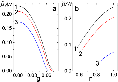
Figure 15: a) The chemical potential versus constant of the electron-phonon interaction g with phonon frequency $\omega_{0}$= 0.01875 at electron concentration n =0.9 and $\alpha$ =0, 0.1 0.3 (curves 1-3, respectively); b) the concentration dependencies of the chemical potential at $\alpha$ =0 and g = 0.01, 0.03 0.06 (curves 1-3, respectively).

Knowing the chemical potential and using Eqs.(47)-(63), it easy to calculate the excitation spectrum and spectral density of the electron cuprate system. Therefore let us write the expression for $\varepsilon_{c.}$ similar to Eq.(74) that determines the dispersion equation

$$-\varepsilon_{c.}(\Omega_{\textbf{k}})=-\frac{{4(\Omega_{\textbf{k}}+\tilde{\mu})^{2}}}{{L(\Omega_{\textbf{k}})}},$$ (77)

where

$$L(\omega)=(\omega+\tilde{\mu})(1-0.5n)M\left({1,1+\frac{{\omega+\tilde{\mu}}}{{\omega_{0}}}}\right)$$

$$+J_{5}(\omega)+(\omega+\tilde{\mu})^{2}{\mathop{\rm Re}\nolimits}P_{46}(\omega)$$ (78)

In particular, along the nodal direction the module of k-momentum as function of resonance frequency is written in form

$$k(\Omega_{{\it k}})=\arccos\left(\frac{-1+\sqrt{1-2\alpha\varepsilon_{c.}(\Omega_{{\it k}})}}{2\alpha}\right)$$ (79)

Apparently, the momentum ${k_{F}}$ on the Fermi surface is determined from condition ${k_{F}=k(0)}$. If $-\varepsilon_{c.}(0)=-\varepsilon_{F}<0$ then we have the electron Fermi surface and hole one otherwise. A given statement may be disrupted for $\alpha\neq 0$.

In Fig.16 the dependence $-\varepsilon_{F}$ versus n at g=0.03 and $\alpha$=0 is presented. It is evident from Fig.16 that the hole Fermi surface is changed to electron one in a certain area of the electron concentrations.

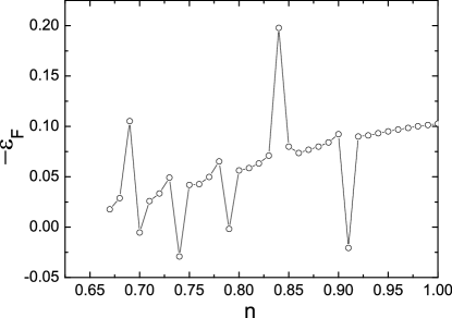
Figure 16: The dependence of the critical parameter $-\varepsilon_{F}$ on electron concentration at g=0.03 and $\alpha$=0.

In Fig.17 the electron excitation frequency-momentum dispersion curves in a wide area of a spectrum (a) and near the Fermi level (b) along the nodal direction at n=0.9, $\alpha$=0 for different values of g are depicted. One can see from Fig.17 that the radical rebuilding of the excitation spectrum occurs with increasing the electron-phonon binding energy. It is a result of the appearance of polaron bands which are grouped near the frequencies to be multiple the phonon frequency $\omega_{0}$. It should be noted that there is a weak dependence of resonance frequency on k at g=0.06 (see Fig.17 a, curve 4) that is in agreement with ARPES experimental data 11 .

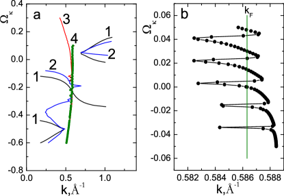
Figure 17: a) The excitation frequency-momentum dispersion along the nodal direction at n=0.9, $\alpha$=0 for values of g =0, 0.01, 0.03 and 0.06 (curves 1-4, respectively). The points in Fig. correspond to $\alpha$=0.1 and g=0.06; b) a fine structure of excitation spectrum a) at g =0.06. The vertical line corresponds to wave vector ${k=k_{F}}$ on the Fermi surface.

The fine spectrum structure near the Fermi level shows an enough drastic frequency change with a small change of k. In particular, below the Fermi level the first kink is observed at $\Omega_{{\it k}}\sim-\omega_{0}$, i.e. at a frequency of the typical optic phonon mode. This is in agreement with experimental data $\Omega_{{\it k}}$${\sim}$50-70 mEv 10 ; 24 for bandwidth ${W\sim}4eV$. A somewhat different kink direction from right to left may be changed by sign replacement of hopping integral, i.e. t on -t . Also, when the kink is observed the value of momentum ${k_{th.}\sim}$0.586 $\AA^{-1}$ . It is in accordance with experiment ${k_{exp.}\sim}$0.41 $\AA^{-1}$ 1 ; 9 ; 10 if to put $k_{th.}$/$\sqrt{2}$. Seemingly, the maximal value of the hopping integral t is realized along diagonal of the square lattice. Although, the other factors determining the kink position are not excluded.

A high degree of coherence of excitations near the Fermi level is the distinctive feature of obtained spectrum with polaron bands. Indeed, for a square lattice the excitation spectrum is very diverse at g=0. But the strong low-dimensional fluctuations are responsible for a low degree of coherence of excitations excluding some edge points determined by Im$G(s,\alpha)$. To verify this we write the expression for spectral density generally

$$\begin{array}[]{l}A(k,\,\,\omega)=\frac{1}{\pi}\\ \times\frac{{(\omega+\tilde{\mu})^{4}\beta{\mathop{\rm Im}\nolimits}P_{46}(\omega)}}{{\left[{(\omega+\tilde{\mu})^{2}-t(k)L(\omega)}\right]^{2}+(\omega+\tilde{\mu})^{2}t^{2}(k)\left[{(\omega+\tilde{\mu})^{2}\beta{\mathop{\rm Im}\nolimits}P_{46}(\omega)}\right]^{2}}}\\ \end{array}$$

where $P_{46}(\omega)$ and $L(\omega)$ are determined in subsection A and by Eq.(III.3), respectively.

In Fig.18 the EDC dependencies of spectral density at n=0.9, $\alpha$=0 and g=0.06 ($\tilde{\mu}$ =0.053) are presented for different momentums along the nodal direction near the Fermi wave vector ${k_{F}}$=0.586 $\AA^{-1}$. From Fig.18 it is seen that the sharp peaks are observed on the curve $A({\it k},\,\,\omega)$ for Fermi momentum ${k=k_{F}}$ (see curve 2). Also, the satellite peaks with smaller amplitudes are seen for other energies of excitations. These peaks correspond to points of intersection by straight line ${k=k_{F}}$ of polaron bands which are depicted in Fig.17 a.

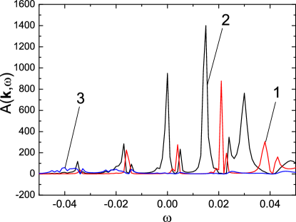
Figure 18: The frequency dependencies of the spectral density at n=0.9, $\alpha$=0, g=0.06 and ${k=k_{F}}$-0.003, ${k=k_{F}}$ and ${k=k_{F}}$ +0.003 (curves 1-3, respectively) for momentums along the nodal direction where ${k=k_{F}}$=0.586 $\AA^{-1}$ and parameter square lattice a${=3.814\AA}$.

It should be noted that a small change of ${k}$ from ${k_{F}}$ gives a sharp decreasing of the spectral density (see curves 1 and 3 in Fig.18). The coherence of excitations is reduced as the electron-phonon binding is weakened. Also, a correlation gap arises on the Fermi level for sufficiently small values of g (see Fig.17 a).

Thus, for cuprates in the strong-coupling polaron limit the hole or electron Fermi surface is realized, depending on electron concentration and value of g. A spectral density reflects the high degree of excitation coherence near the Fermi level. The availability of the narrow polaron bands, which are grouped near the frequencies to be multiple the phonon frequency $\omega_{0}$, results in a sharp resonance frequency changing along the nodal direction of the momentum. It explains the origin of kink to be observed at energy $\omega\sim-\omega_{0}$ from ARPES data for bismuth cuprates.

IV Conclusions

For strongly correlated electron subsystem with Holstein’s polarons within the framework of diagrammatic method of perturbation theory a generalization for approximation Hubbard-I was made. Strong electron correlations narrow a valency band in a doped Mott insulator that results in radically difference one from metal. The Lang-Firsov unitary transform was made to separate fermionic and bosonic subsystems. It allows to evaluate all polaron bands each of which are formed near the Einstein mode.

In the first nonvanishing approximation of time-dependent perturbation theory with respect to the inverse effective radius of interaction we account for influence of inelastic electron-electron scattering on chemical potential and time-ordered Green’s function. Taking into account a low-dimensional character of system it was obtained that all peculiarities of excitation spectrum and damping are determined by lattice Green’ function for which there is a closed analytic expression. An influence of electron concentration and next-nearest-neighbor hopping integral on chemical potential, spectrum structure and spectral density has been determined. In particular, with well-defined electron concentrations the correlation gap in spectrum arises on the Fermi level. In the absence of this gap the Fermi surface can have the hole as well as electron character depending on electron concentration and influence of the next-nearest-neighbor hopping integral. In spite of the complicated picture of excitation spectrum the spectral density shows a relatively low degree of coherence. It is connected with a low space dimension of the system where the role of quantum fluctuations are important.

In addition to the previously considered approach the inclusion of the electron-phonon interaction allowed to reveal the main peculiarities of spectrum. They are in a good correspondence to experimental ARPES data. Indeed, in a wide area of frequencies a weak momentum dependence of spectrum along the nodal direction was found that is in agreement with experiment [11]. The spectral density turned out to be typical for strongly coherent excitations near the Fermi level in case of the strong electron-phonon binding. It simplifies the experimental measure the Fermi surface. Thus, the electron-phonon interaction partially suppresses low-dimensional quantum fluctuations and strengthen the coherence of the excitations. From the above analysis of a fine structure of polaron spectrum one can conclude that the observed kink 9 ; 10 appears at frequency of characteristic optical phonon mode in the vicinity of which the polaron band is formed.

References

• (1) J.R. Schrieffer and J.S. Brooks, (Eds.), Handbook of High-Temperature Superconductivity. Theory and Experiment, (Springer, New York, 2007 ), p.627.
• (2) W. Zhang, Photoemission Spectroscopy on High Temperature Superconductor, (Springer-Verlag: Berlin, Heidelberg, 2013), p.139.
• (3) R.N. Bhattacharya, M.P. Paranthaman, (Eds.), High Temperature Superconductors, (Wiley-VCH, 2010), p.227.
• (4) W.E. Pickett, Phys.ย Rev.ย Bย 36, 381 (1987).
• (5) V. Anisimov, Yu. Izyumov, Electronic Structure of Strongly Correlated Materials, (Springer: Heidelberg, 2010), p.288.
• (6) S. Verga, A. Knigavko, and F. Marsiglio, Phys.ย Rev.ย Bย 67, 054503 (2003).
• (7) A. W. Sandvik, D. J. Scalapino, and N. E. Bickers, Phys.ย Rev.ย Bย 69, 094523 (2004).
• (8) Lin Zhao, Jing Wang, Junren Shi, Wentao Zhang, Haiyun Liu, Jianqiao Meng, Guodong Liu, Xiaoli Dong, Jun Zhang, Wei Lu, Guiling Wang, Yong Zhu, Xiaoyang Wang, Qinjun Peng, Zhimin Wang, Shenjin Zhang, Feng Yang, Chuangtian Chen, Zuyan Xu, and X. J. Zhou, Phys.ย Rev.ย Bย 83, 184515 (2011).
• (9) T. Valla, A. V. Fedorov, P.D. Johnson, B. O. Wells, S. L. Hulbert, Q. Li, G. D. Gu, N. Koshizuka, Scienceย 285, 2110 (1999).
• (10) P.V. Bogdanov, A. Lanzara, S. A. Kellar, X. J. Zhou, E. D. Lu, W. J. Zheng, G. Gu, J.-I. Shimoyama, K. Kishio, H. Ikeda, R. Yoshizaki, Z. Hussain, and Z. X. Shen, Phys.ย Rev.ย Lett.ย 85, 2581 (2000).
• (11) B. P. Xie, K. Yang, D.W. Shen, J. F. Zhao, H.W. Ou, J. Wei, S.Y. Gu, M. Arita, S. Qiao, H. Namatame, M. Taniguchi, N. Kaneko, H. Eisaki, K. D. Tsuei, C. M. Cheng, I. Vobornik, J. Fujii, G. Rossi, Z. Q. Yang, and D. L. Feng, Phys.ย Rev.ย Lett.ย 98, 147001 (2007).
• (12) J. Hubbard, Proc.ย R.ย Soc.ย Lond.ย Aย 276, 238 (1963).
• (13) W.F. Brinkman and T.M.Rice, Phys.ย Rev.ย Bย 2, 1324 (1970).
• (14) E.E. Zubov, V.P. Dyakonov and H. Szymczak, J.ย Phys.:ย Condens.ย Matterย  18, 6699 (2006).
• (15) E.E. Zubov, Physicaย Cย  497, 67 (2014).
• (16) M.L. Kuliฤ‰, Physics Reports 338, 1 (2000).
• (17) E.G. Maksimov, M.L. Kuliฤ‰ and O.V. Dolgov, Adv.ย Cond.ย Matt.ย Phys.ย  2010, 1 (2010).
• (18) I.G. Lang and Yu.A. Firsov, Zh.ย Exp.ย Theor.ย Fiz.ย 43, 1843 (1962)(Sov.ย Phys. ย JETP 16, 1301 (1963)).
• (19) G.D. Mahan, Many Particle Physics, (Plenum, New York, 1990), p.793.
• (20) M. Abramowitz and C.A. Stegun, (Eds.), Handbook of Mathematical Functions with Formulas, Graphs, and Mathematical Tables , (Dover, New York, 1972), p.1046.
• (21) A. Gil, W. Koepf and J. Segura, Numerical Algorithms 36, 113 (2004).
• (22) T. Morita, T. Horiguchi, Journ.ย Math.ย Phys.ย  12, 986 (1971).
• (23) E.E. Zubov, Theoreticalย and Mathematicalย Physicsย 105, 1442 (1995).
• (24) S Ideta, T Yoshida, M Hashimoto, A Fujimori, H Anzai, A Ino, M Arita, H Namatame, M Taniguchi, K Takashima, K M Kojima and S Uchida, J.ย Phys.:ย Conf.ย Ser.ย  428, 012039 (2013).