Finite Element Approximation of the Laplace-Beltrami Operator on a Surface with Boundary

Abstract

We develop a finite element method for the Laplace-Beltrami operator on a surface with boundary and nonhomogeneous Dirichlet boundary conditions. The method is based on a triangulation of the surface and the boundary conditions are enforced weakly using Nitsche’s method. We prove optimal order a priori error estimates for piecewise continuous polynomials of order $k\geq 1$ in the energy and $L^{2}$ norms that take the approximation of the surface and the boundary into account.

Subject Classification Codes:

65M60, 65M85.

Keywords:

Laplace-Beltrami operator, surface with boundary, Nitsche’s method, a priori error estimates.

1 Introduction

Finite element methods for problems on surfaces have been rapidly developed starting with the seminal work of Dziuk [11]. Different approaches have been developed including methods based on meshed surfaces, [1], [9], [10], [16], and methods based on implicit or embedded approaches, [5], [19], [20], see also the overview articles [12] and [3], and the references therein. So far the theoretical developments are, however, restricted to surfaces without boundary.

In this contribution we develop a finite element method for the Laplace-Beltrami operator on a surface which has a boundary equipped with a nonhomogeneous Dirichlet boundary condition. The results may be readily extended to include Neumann conditions on part of the boundary, which we also comment on in a remark. The method is based on a triangulation of the surface together with a Nitsche formulation [18] for the Dirichlet boundary condition. Polynomials of order $k$ are used both in the interpolation of the surface and in the finite element space. Our theoretical approach is related to the recent work [4] where a priori error estimates for a Nitsche method with so called boundary value correction [2] is developed for the Dirichlet problem on a (flat) domain in $\mathbb{R}^{n}$. We also mention the work [21] where the smooth curved boundary of a domain in $\mathbb{R}^{2}$ is interpolated and Dirichlet boundary conditions are strongly enforced in the nodes.

Provided the error in the position of the approximate surface and its boundary is (pointwise) of order $k+1$ and the error in the normals/tangents is of order $k$, we prove optimal order error estimates in the $L^{2}$ and energy norms. No additional regularity of the exact solution, compared to standard estimates, is required. The proof is based on a Strang lemma which accounts for the error caused by approximation of the solution, the surface, and the boundary. Here the discrete surface is mapped using a closest point mapping onto a surface containing the exact surface. The error caused by the boundary approximation is then handled using a consistency argument. Special care is required to obtain optimal order $L^{2}$ error estimates and a refined Aubin-Nitsche duality argument is used which exploits the fact that the dual problem is small close to the boundary since the dual problem is equipped with a homogeneous Dirichlet condition.

The outline of the paper is as follows: In Section 2 we formulate the model problem and finite element method. We also formulate the precise assumptions on the approximation of the surface and its boundary. In Section 3 we develop the necessary results to prove our main error estimates. In Section 4 we present numerical results confirming our theoretical findings.

2 Model Problem and Method

2.1 The Surface

Let, $\Gamma\subset\Gamma_{0}$ be a surface with smooth boundary $\partial\Gamma$, where $\Gamma_{0}$ is a smooth closed connected hypersurface embedded in $\mathbb{R}^{3}$. We let $n$ be the exterior unit normal to $\Gamma_{0}$ and $\nu$ be the exterior unit conormal to $\partial\Gamma$, i.e. $\nu(x)$ is orthogonal both to the tangent vector of $\partial\Gamma$ at $x$ and the normal $n(x)$ of $\Gamma_{0}$. For $\Gamma_{0}$, we denote its associated signed distance function by $\rho$ which satisfies $\nabla\rho=n$, and we define an open tubular neighborhood of $\Gamma_{0}$ by $U_{\delta}(\Gamma_{0})=\{x\in\mathbb{R}^{3}:|\rho(x)|<\delta\}$ with $\delta>0$. Then there is $\delta_{0,\Gamma_{0}}>0$ such that the closest point mapping $p:U_{\delta_{0,\Gamma_{0}}}(\Gamma_{0})\rightarrow\Gamma_{0}$ assigns precisely one point on $\Gamma_{0}$ to each point in $U_{\delta_{0,\Gamma_{0}}}(\Gamma_{0})$. The closest point mapping takes the form

$$p:U_{\delta_{0,\Gamma_{0}}}(\Gamma_{0})\ni x\mapsto x-\rho(x)n\circ p(x)\in\Gamma_{0}$$ (2.1)

For the boundary curve $\partial\Gamma$, let $\rho_{\partial\Gamma}$ be the distance function to the curve $\partial\Gamma$, and $p_{\partial\Gamma}$ be the associated closest point mapping giving raise to the tubular neighborhood $U_{\delta}(\partial\Gamma)=\{x\in\mathbb{R}^{3}\,:\,|\rho_{\partial\Gamma}(x)|<\delta\}$. Note that there is $\delta_{0,\partial\Gamma}>0$ such that the closest point mapping $p_{\partial\Gamma}:U_{\delta_{0,\partial\Gamma}}(\partial\Gamma)\rightarrow\partial\Gamma$ is well defined. Finally, we let $\delta_{0}=\min(\delta_{0,\Gamma_{0}},\delta_{0,\partial\Gamma})$ and introduce $U_{\delta_{0}}(\Gamma)=\{x\in\mathbb{R}^{3}\,:\,|\rho(x)|\lesssim\delta_{0}\}$.

Remark 2.1

Clearly we may take $\Gamma_{0}$ to be a surface that is only slightly larger than $\Gamma$ but for simplicity we have taken $\Gamma_{0}$ closed in order to obtain a well defined closest point mapping without boundary effects in a convenient way.

Remark 2.2

Our theoretical developments covers a smooth orientable hypersurface with smooth boundary in $\mathbb{R}^{n}$, also for $n>3$.

2.2 The Problem

Tangential Calculus.

For each $x\in\Gamma_{0}$ let $T_{x}(\Gamma_{0})=\{y\in\mathbb{R}^{3}:(y,n(x))_{\mathbb{R}^{3}}=0\}$ and $N_{x}(\Gamma)=\{y\in\mathbb{R}^{3}:\alpha n(x)),\alpha\in\mathbb{R}\}$ be the tangent and normal spaces equipped with the inner products $(v,w)_{T_{x}(\Gamma_{0})}=(v,w)_{\mathbb{R}^{3}}$ and $(v,w)_{N_{x}(\Gamma_{0})}=(v,w)_{\mathbb{R}^{3}}$. Let $P_{\Gamma}:\mathbb{R}^{3}\rightarrow T_{x}(\Gamma_{0})$ be the projection of $\mathbb{R}^{3}$ onto the tangent space given by $P_{\Gamma}=I-n\otimes n$ and let $Q_{\Gamma}:\mathbb{R}^{3}\rightarrow N_{x}(\Gamma_{0})$ be the orthogonal projection onto the normal space given by $Q_{\Gamma}=I-P_{\Gamma}=n\otimes n$. The tangent gradient is defined by $\nabla_{\Gamma}v=P_{\Gamma}\nabla v$. For a tangential vector field $w$, i.e. a mapping $w:\Gamma_{0}\ni x\mapsto w(x)\in T_{x}(\Gamma_{0})$, the divergence is defined by $\text{div}_{\Gamma}w=\text{tr}(w\otimes\nabla_{\Gamma})$. Then the Laplace-Beltrami operator is given by $\Delta_{\Gamma}v=\text{div}_{\Gamma}\nabla_{\Gamma}v$. Note that we have Green’s formula

$$(-\Delta_{\Gamma}v,w)=(\nabla_{\Gamma}v,\nabla_{\Gamma}w)_{\Gamma}-(\nu\cdot\nabla_{\Gamma}v,w)_{\partial\Gamma}$$ (2.2)

Model Problem.

Find $u:\Gamma\rightarrow\mathbb{R}$ such that

$$-\Delta_{\Gamma}u =f\qquad \Gamma$$ in (2.3)

$$u =g\qquad \partial\Gamma$$ on (2.4)

where $f\in H^{-1}(\Gamma)$ and $g\in H^{1/2}(\partial\Gamma)$ are given data. Thanks to the Lax-Milgram theorem, there is a unique solution $u\in H^{1}(\Gamma)$ to this problem. Moreover, we have the elliptic regularity estimate

$$\|u\|_{H^{s+2}(\Gamma)}\lesssim\|f\|_{H^{s}(\Gamma)}+\|g\|_{H^{s+3/2}(\Gamma)},\qquad s\geq-1$$ (2.5)

since $\Gamma$ and $\partial\Gamma$ are smooth. Here and below we use the notation $\lesssim$ to denote less or equal up to a constant. We also adopt the standard notation $H^{s}(\omega)$ for the Sobolev space of order $s$ on $\omega\subset\Gamma_{0}$ with norm $\|\cdot\|_{H^{s}(\omega)}$. For $s=0$ we use the notation $L^{2}(\omega)$ with norm $\|\cdot\|_{\omega}$, see [22] for a detailed description of Sobolev spaces on smooth manifolds with boundary.

2.3 The Discrete Surface and Finite Element Spaces

To formulate our finite element method for the boundary value problem (2.3)–(2.4) in the next section, we here summarize our assumptions on the approximation quality of the discretization of $\Gamma$.

Discrete Surface.

Let $\{\Gamma_{h},\,h\in(0,h_{0}]\}$ be a family of connected triangular surfaces with mesh parameter $h$ that approximates $\Gamma$ and let $\mathcal{K}_{h}$ be the mesh associated with ${\Gamma_{h}}$. For each element $K\in\mathcal{K}$, there is a bijection $F_{K}:\widehat{K}\rightarrow K$ such that $F_{K}\in[\widehat{V}_{k}]^{3}=[P_{k}(\widehat{K})]^{3}$, where $\widehat{K}$ is a reference triangle in $\mathbb{R}^{2}$ and $P_{k}(\widehat{K})$ is the space of polynomials of order less or equal to $k$. We assume that the mesh is quasi-uniform. For each $K\in\mathcal{K}_{h}$, we let $n_{h}|_{K}$ be the unit normal to $\Gamma_{h}$, oriented such that $(n_{h},n\circ p)_{\mathbb{R}^{3}}>0$. On the element edges forming $\partial\Gamma_{h}$, we define $\nu_{\partial\Gamma_{h}}$ to be the exterior unit conormal to $\partial\Gamma_{h}$, i.e. $\nu_{\partial\Gamma_{h}}(x)$ is orthogonal both to the tangent vector of $\partial\Gamma_{h}$ at $x$ and the normal $n_{h}(x)$ of $\Gamma_{h}$. We also introduce the tangent projection $P_{{\Gamma_{h}}}=I-n_{h}\otimes n_{h}$ and the normal projection $Q_{{\Gamma_{h}}}=n_{h}\otimes n_{h}$, associated with ${\Gamma_{h}}$.

Geometric Approximation Property.

We assume that $\{\Gamma_{h},h\in(0,h_{0}]\}$ approximate $\Gamma$ in the following way: for all $h\in(0,h_{0}]$ it holds

$$\Gamma_{h}\subset U_{\delta_{0}}(\Gamma)$$ (2.6)

$$\partial\Gamma_{h}\subset U_{\delta_{0}}(\partial\Gamma)$$ (2.7)

$$\|\rho_{\Gamma}\|_{L^{\infty}({\Gamma_{h}})}\lesssim h^{k+1}$$ (2.8)

$$\|n\circ p_{\Gamma}-n_{h}\|_{L^{\infty}({\Gamma_{h}})}\lesssim h^{k}$$ (2.9)

$$\|\rho_{\partial\Gamma}\|_{L^{\infty}(\partial{\Gamma_{h}})}\lesssim h^{k+1}$$ (2.10)

$$\|\nu\circ p_{\partial\Gamma}-{\color[rgb]{0,0,0}\nu_{\Gamma_{h}}}\|_{L^{\infty}({\Gamma_{h}})}\lesssim h^{k}$$ (2.11)

Note that it follows that we also have the estimate

$$\|t_{\partial\Gamma}\circ p_{\partial\Gamma}-t_{\partial{\Gamma_{h}}}\|_{L^{\infty}(\partial{\Gamma_{h}})}\lesssim h^{k}$$ (2.12)

for the unit tangent vectors $t_{\partial\Gamma}$ and $t_{\partial{\Gamma_{h}}}$ of $\partial\Gamma$ and $\partial{\Gamma_{h}}$.

Finite Element Spaces.

Let $V_{h}$ be the space of parametric continuous piecewise polynomials of order $k$ defined on $\mathcal{K}_{h}$, i.e.

$$V_{h}=\{v\in C({\Gamma_{h}},\mathbb{R})\,:\,v|_{K}\in\widehat{V}_{k}\circ F_{K}^{-1}\}$$ (2.13)

where $\widehat{V}_{k}=P_{k}(\widehat{K})$ is the space of polynomials of order less or equal to $k$ defined on the reference triangle $\widehat{K}$ defined above.

2.4 The Finite Element Method

The finite element method for the boundary value problem (2.3)–(2.4) takes the form: find $u_{h}\in V_{h}$ such that

$$a_{{\Gamma_{h}}}(u_{h},v)=l_{{\Gamma_{h}}}(v),\qquad\forall v\in V_{h}$$ (2.14)

where

$$a_{{\Gamma_{h}}}(v,w) =(\nabla_{\Gamma_{h}}v,\nabla_{\Gamma_{h}}w)_{\Gamma_{h}}$$ (2.15)

$$\qquad-(\nu_{\partial{\Gamma_{h}}}\cdot\nabla_{\Gamma_{h}}v,w)_{\partial\Gamma_{h}}-(v,\nu_{\partial{\Gamma_{h}}}\cdot\nabla_{\Gamma_{h}}w)_{\partial\Gamma_{h}}$$

$$\qquad+\beta h^{-1}(v,w)_{\partial\Gamma_{h}}$$

$$l_{{\Gamma_{h}}}(w) =(f\circ p,w)_{\Gamma_{h}}-(g\circ p_{\partial\Gamma},\nu_{\partial{\Gamma_{h}}}\cdot\nabla_{\Gamma_{h}}w)_{\partial\Gamma_{h}}+\beta h^{-1}(g\circ p_{\partial\Gamma},w)_{\partial\Gamma_{h}}$$ (2.16)

Here $\beta>0$ is a parameter, and $f$ is extended from $\Gamma$ to $\Gamma\cup p(\Gamma_{h})\subset\Gamma_{0}$ in such a way that $f\in H^{m}(\Gamma\cup p({\Gamma_{h}}))$ and

$$\|f\|_{H^{m}(\Gamma\cup p({\Gamma_{h}}))}\lesssim\|f\|_{H^{m}(\Gamma)}$$ (2.17)

where $m=0$ for $k=1$ and $m=1$ for $k\geq 2$.

Remark 2.3

Note that in order to prove optimal a priori error estimates for piecewise polynomials of order $k$ we require $u\in H^{k+1}(\Gamma)$ and thus $f\in H^{k-1}(\Gamma)$. For $k=1$ we have $f\in L^{2}(\Gamma)$ and for $k\geq 2$ we require $f\in H^{k-1}(\Gamma)\subseteq H^{1}(\Gamma)$. Thus we conclude that (2.17) does not require any additional regularity compared to the standard situation. We will also see in Section 3.4 below that there indeed exists extensions of functions that preserve regularity.

3 A Priori Error Estimates

We derive a priori error estimates that take both the approximation of the geometry and the solution into account. The main new feature is that our analysis also takes the approximation of the boundary into account.

3.1 Lifting and Extension of Functions

We collect some basic facts about lifting and extensions of functions, their derivatives, and related change of variable formulas, see for instance [5], [10], and [11], for further details.

• For each function $v$ defined on $\Gamma_{0}$ we define the extension

  $$v^{e}=v\circ p$$ (3.1)

  to $U_{\delta_{\Gamma_{0}}}(\Gamma_{0})$. For each function $v$ defined on ${\Gamma_{h}}$ we define the lift to ${\Gamma_{h}^{l}}=p({\Gamma_{h}})\subset\Gamma_{0}$ by

  $$v^{l}\circ p=v$$ (3.2)

  Here and below we use the notation $\omega^{l}=p(\omega)\subset\Gamma_{0}$ for any subset $\omega\subset{\Gamma_{h}}$.

• The derivative $dp:T_{x}({\Gamma_{h}})\rightarrow T_{p(x)}(\Gamma)$ of the closest point mapping $p:{\Gamma_{h}}\rightarrow\Gamma_{0}$ is given by

  $$dp(x)=P_{\Gamma}(p(x))P_{{\Gamma_{h}}}(x)+\rho(x)\mathcal{H}(x)P_{{\Gamma_{h}}}(x)$$ (3.3)

  where $T_{x}(\Gamma)$ and $T_{p(x)}({\Gamma_{h}})$ are the tangent spaces to $\Gamma$ at $x\in\Gamma$ and to ${\Gamma_{h}}$ at $p(x)\in{\Gamma_{h}}$, respectively. Furthermore, $\mathcal{H}(x)=\nabla\otimes\nabla\rho(x)$ is the $\Gamma$ tangential curvature tensor which satisfies the estimate $\|\mathcal{H}\|_{L^{\infty}(U_{\delta}(\Gamma_{0}))}\lesssim 1$, for some small enough $\delta>0$, see [14] for further details. We use $B$ to denote a matrix representation of the operator $dp$ with respect to an arbitrary choice of orthonormal bases in $T_{x}({\Gamma_{h}})$ and $T_{p(x)}(\Gamma)$.

• Gradients of extensions and lifts are given by

  $$\nabla_{\Gamma_{h}}v^{e}=B^{T}\nabla_{\Gamma}v,\qquad\nabla_{\Gamma}v^{l}=B^{-T}\nabla_{\Gamma_{h}}v$$ (3.4)

  where the gradients are represented as column vectors and the transpose $B^{T}:T_{p(x)}(\Gamma)\rightarrow T_{x}(\Gamma_{0})$ is defined by $(Bv,w)_{T_{p(x)}(\Gamma)}=(v,B^{T}w)_{T_{x}(\Gamma_{0})}$, for all $v\in T_{x}({\Gamma_{h}})$ and $w\in T_{p(x)}(\Gamma)$.

• We have the following estimates

  $$\|B\|_{L^{\infty}(\Gamma_{h})}\lesssim 1,\qquad\|B^{-1}\|_{L^{\infty}(\Gamma)}\lesssim 1$$ (3.5)

• We have the change of variables formulas

  $$\int_{\omega^{l}}g^{l}d\Gamma=\int_{\omega}g|B|d\Gamma_{h}$$ (3.6)

  for a subset $\omega\subset{\Gamma_{h}}$, and

  $$\int_{\gamma^{l}}g^{l}d\Gamma=\int_{\gamma}g|B_{\partial{\Gamma_{h}}}|d\Gamma_{h}$$ (3.7)

  for a subset $\gamma\subset\partial\Gamma_{h}$. Here $|B|$ denotes the absolute value of the determinant of $B$ (recall that we are using orthonormal bases in the tangent spaces) and $|B_{\partial\Gamma_{h}}|$ denotes the norm of the restriction $B_{\partial{\Gamma_{h}}}:T_{x}(\partial{\Gamma_{h}})\rightarrow T_{p(x)}(\partial{\Gamma_{h}^{l}})$ of $B$ to the one dimensional tangent space of the boundary curve. We then have the estimates

  $$|\,|B|-1\,|\lesssim h^{k+1},\qquad|\,|B^{-1}|-1\,|\lesssim h^{k+1}$$ (3.8)

  and

  $$|\,|B_{\partial\Gamma_{h}}|-1\,|\lesssim h^{k+1},\qquad|\,|B^{-1}_{\partial\Gamma_{h}}|-1\,|\lesssim h^{k+1}$$ (3.9)

  Estimate (3.8) appear in several papers, see for instance [10]. Estimate (3.9) is less common but appears in papers on discontinuous Galerkin methods on surfaces, see [6], [9], and [16]. For completeness we include a simple proof of (3.9).

  Verification of (3.9).

  Let $\gamma_{\Gamma_{h}}:[0,a)\rightarrow\partial{\Gamma_{h}}\subset\mathbb{R}^{3}$ be a parametrization of the curve $\partial{\Gamma_{h}}$ in $\mathbb{R}^{3}$, with $a$ some positive real number. Then $p\circ\gamma_{\Gamma_{h}}(t)$, $t\in[0,a)$, is a parametrization of $\partial{\Gamma_{h}^{l}}$. We have

  $$|d_{t}\gamma_{\Gamma_{h}^{l}}|_{\mathbb{R}^{3}}=|d_{t}p\circ\gamma_{\Gamma_{h}}|_{\mathbb{R}^{3}}=|dpd_{t}\gamma_{\Gamma_{h}}|_{\mathbb{R}^{3}}=|B_{\partial{\Gamma_{h}}}||d_{t}\gamma_{\Gamma_{h}}|_{\mathbb{R}^{3}}$$ (3.10)

  and

  $$|dpd_{t}\gamma_{\Gamma_{h}}|_{\mathbb{R}^{3}}-|d_{t}\gamma_{\Gamma_{h}}|_{\mathbb{R}^{3}} =|(P_{\Gamma}+\rho\mathcal{H})d_{t}\gamma_{\Gamma_{h}}|_{\mathbb{R}^{3}}-|d_{t}\gamma_{\Gamma_{h}}|_{\mathbb{R}^{3}}$$ (3.11)

  $$=\underbrace{|P_{\Gamma}d_{t}\gamma_{\Gamma_{h}}|_{\mathbb{R}^{3}}-|d_{t}\gamma_{\Gamma_{h}}|_{\mathbb{R}^{3}}}_{\bigstar=O(h^{2k})}+O(h^{k+1})$$ (3.12)

  Here we estimated $\bigstar$ by first using the identity

  $$|P_{\Gamma}d_{t}\gamma_{\Gamma_{h}}|^{2} =|d_{t}\gamma_{\Gamma_{h}}-Q_{\Gamma}d_{t}\gamma_{\Gamma_{h}}|^{2}$$ (3.13)

  $$=|d_{t}\gamma_{\Gamma_{h}}|^{2}-2d_{t}\gamma_{\Gamma_{h}}\cdot Q_{\Gamma}d_{t}\gamma_{\Gamma_{h}}+|Q_{\Gamma}d_{t}\gamma_{\Gamma_{h}}|^{2}$$ (3.14)

  $$=|d_{t}\gamma_{\Gamma_{h}}|^{2}-|Q_{\Gamma}d_{t}\gamma_{\Gamma_{h}}|^{2}$$ (3.15)

  $$\geq(1-Ch^{2k})|d_{t}\gamma_{\Gamma_{h}}|^{2}$$ (3.16)

  and then using the estimate $|(1+\delta)^{1/2}-1|\lesssim|\delta|$, for $-1\leq\delta$, to conclude that

  $$\Big{|}|P_{\Gamma}d_{t}\gamma_{\Gamma_{h}}|-|d_{t}\gamma_{\Gamma_{h}}|\Big{|}\lesssim h^{2k}|d_{t}\gamma_{\Gamma_{h}}|$$ (3.17)

• The following equivalences of norms hold (uniformly in $h$)

  $$\|v\|_{H^{m}({\Gamma_{h}^{l}})}\sim\|v^{e}\|_{H^{m}({\Gamma_{h}})},\qquad m=0,1,\qquad v\in H^{m}(\Gamma)$$ (3.18)

  $$\|v^{l}\|_{H^{m}({\Gamma_{h}^{l}})}\sim\|v\|_{H^{m}({\Gamma_{h}})},\qquad m=0,1,\qquad v\in H^{m}({\Gamma_{h}})$$ (3.19)

  These estimates follow from the identities for the gradients (3.4), the uniform bounds (3.5) of $B$, and the bounds (3.8) for the determinant $|B|$.

3.2 Norms

We define the norms

$$|||v|||^{2}_{{\Gamma_{h}}}=\|\nabla_{\Gamma_{h}}v\|^{2}_{{\Gamma_{h}}}+|||v|||^{2}_{\partial{\Gamma_{h}}},\qquad|||v|||^{2}_{\partial{\Gamma_{h}}}=h\|\nu_{\partial{\Gamma_{h}}}\cdot\nabla_{\Gamma_{h}}v\|^{2}_{\partial{\Gamma_{h}}}+h^{-1}\|v\|^{2}_{\partial{\Gamma_{h}}}$$ (3.20)

$$|||v|||^{2}_{{\Gamma_{h}^{l}}}=\|\nabla_{\Gamma}v\|^{2}_{{\Gamma_{h}^{l}}}+|||v|||^{2}_{\partial{\Gamma_{h}^{l}}},\qquad|||v|||^{2}_{\partial{\Gamma_{h}^{l}}}=h\|\nu_{\partial{\Gamma_{h}^{l}}}\cdot\nabla_{\Gamma}v\|^{2}_{\partial{\Gamma_{h}^{l}}}+h^{-1}\|v\|^{2}_{\partial{\Gamma_{h}^{l}}}$$ (3.21)

Here $\nu_{\partial{\Gamma_{h}^{l}}}$ denotes the unit exterior conormal to $\partial{\Gamma_{h}^{l}}$; that is, $\nu_{\partial{\Gamma_{h}^{l}}}$ is a tangent vector to $\Gamma_{0}$, which is orthogonal to the curve ${\Gamma_{h}^{l}}$ and exterior to ${\Gamma_{h}^{l}}$. Then the following equivalences hold

$$|||v^{l}|||_{\Gamma_{h}^{l}}\sim|||v|||_{\Gamma_{h}},\qquad|||v^{l}|||_{\partial{\Gamma_{h}^{l}}}\sim|||v|||_{\partial{\Gamma_{h}}},\qquad v\in V({\Gamma_{h}})$$ (3.22)

$$|||v|||_{\Gamma_{h}^{l}}\sim|||v^{e}|||_{\Gamma_{h}},\qquad|||v|||_{\partial{\Gamma_{h}^{l}}}\sim|||v^{e}|||_{\partial{\Gamma_{h}}},\qquad v\in V({\Gamma_{h}^{l}})$$ (3.23)

Here $V({\Gamma_{h}})=\{v\in C({\Gamma_{h}})\,:\,v|_{K}\in H^{3/2}(K),K\in\mathcal{K}_{h}\}$ and $V({\Gamma_{h}^{l}})=V^{l}({\Gamma_{h}})$. Note that $V_{h}\subset V({\Gamma_{h}})$.

Remark 3.1

We will see that it is convenient to have access to the norms $|||\cdot|||_{\partial{\Gamma_{h}}}$ and $|||\cdot|||_{\partial{\Gamma_{h}^{l}}}$, involving the boundary terms since that allows us to take advantage of stronger control of the solution to the dual problem, which is used in the proof of the $L^{2}$ error estimate, see Theorem 3.2, in the vicinity of the boundary.

Verification of (3.22).

In view of (3.19) it is enough to verify the equivalence $|||v^{l}|||_{\partial{\Gamma_{h}^{l}}}\sim|||v|||_{\partial{\Gamma_{h}}}$, between the boundary norms. First we have using a change of domain of integration from $\partial{\Gamma_{h}^{l}}$ to $\partial{\Gamma_{h}}$ and the bound (3.9),

$$h^{-1}\|v^{l}\|^{2}_{\partial{\Gamma_{h}^{l}}}=h^{-1}(v^{l},v^{l})_{\partial{\Gamma_{h}^{l}}}=h^{-1}(v,v|B_{\partial{\Gamma_{h}}}|)_{\partial{\Gamma_{h}}}\sim h^{-1}\|v\|^{2}_{\partial{\Gamma_{h}}}$$ (3.24)

Next we have the identity

$$\nu_{\partial{\Gamma_{h}^{l}}}\cdot\nabla_{\Gamma}v^{l}=\nu_{\partial{\Gamma_{h}^{l}}}\cdot B^{-T}\nabla_{\Gamma_{h}}v=B^{-1}\nu_{\partial{\Gamma_{h}^{l}}}\cdot\nabla_{\Gamma_{h}}v$$ (3.25)

and thus using the uniform boundedness of $B^{-1}$ we obtain by changing domain of integration from $\partial{\Gamma_{h}^{l}}$ to $\partial{\Gamma_{h}}$, using (3.9), and then splitting $\nabla_{\Gamma_{h}}v$ into components normal and tangent to $\partial{\Gamma_{h}}$,

$$\|\nu_{\partial{\Gamma_{h}^{l}}}\cdot\nabla_{\Gamma}v^{l}\|^{2}_{\partial{\Gamma_{h}^{l}}} \lesssim\|\nabla_{\Gamma_{h}}v\|^{2}_{\partial{\Gamma_{h}}}$$ (3.26)

$$=\|\nu_{\partial{\Gamma_{h}}}\cdot\nabla_{\Gamma_{h}}v\|^{2}_{\partial{\Gamma_{h}}}+\|t_{\partial{\Gamma_{h}}}\cdot\nabla_{\Gamma_{h}}v\|^{2}_{\partial{\Gamma_{h}}}$$ (3.27)

$$\lesssim\|\nu_{\partial{\Gamma_{h}}}\cdot\nabla_{\Gamma_{h}}v\|^{2}_{\partial{\Gamma_{h}}}+h^{-2}\|v\|^{2}_{\partial{\Gamma_{h}}}$$ (3.28)

$$\lesssim h^{-1}|||v|||^{2}_{\partial{\Gamma_{h}}}$$ (3.29)

where $t_{\partial{\Gamma_{h}}}$ is the tangent vector to $\partial{\Gamma_{h}}$ and finally used an inverse estimate to bound the tangent derivative. Multiplying by $h$ we thus have

$$h\|\nu_{\partial{\Gamma_{h}^{l}}}\cdot\nabla_{\Gamma}v^{l}\|^{2}_{\partial{\Gamma_{h}^{l}}}\lesssim|||v|||^{2}_{\partial{\Gamma_{h}}}$$ (3.30)

The converse estimate follows by instead starting from the identity

$$\nu_{\partial{\Gamma_{h}}}\cdot\nabla_{\Gamma_{h}}v=\nu_{\partial{\Gamma_{h}}}\cdot B^{T}B^{-T}\nabla_{\Gamma_{h}}v=B\nu_{\partial{\Gamma_{h}}}\cdot\nabla_{\Gamma}v^{l}$$ (3.31)

and then using similar estimates give

$$h\|\nu_{\partial{\Gamma_{h}}}\cdot\nabla_{\Gamma_{h}}v\|_{\partial{\Gamma_{h}}}^{2}\lesssim|||v^{l}|||_{\partial{\Gamma_{h}^{l}}}^{2}$$ (3.32)

Together (3.24), (3.30), and (3.32) prove the equivalence $|||v^{l}|||_{\partial{\Gamma_{h}^{l}}}\sim|||v|||_{\partial{\Gamma_{h}}}$.

3.3 Coercivity and Continuity

Using standard techniques, see [18] or Chapter 14.2 in [15], we find that $a_{{\Gamma_{h}}}$ is coercive

$$|||v|||_{{\Gamma_{h}}}^{2}\lesssim a_{{\Gamma_{h}}}(v,v)\qquad\forall v\in V_{h}$$ (3.33)

provided $\beta>0$ is large enough. Furthermore, it follows directly from the Cauchy-Schwarz inequality that $a_{\Gamma_{h}}$ is continuous

$$a_{\Gamma_{h}}(v,w)\lesssim|||v|||_{\Gamma_{h}}|||w|||_{\Gamma_{h}}\qquad\forall v,w\in V({\Gamma_{h}})$$ (3.34)

Existence and uniqueness of the solution $u_{h}$ to the finite element problem (2.14) follows directly from the Lax-Milgram lemma.

3.4 Extension and Interpolation

Next, we briefly review the fundamental interpolation estimates which will be used throughout the remaining work.

Extension.

We note that there is an extension operator $E:H^{s}(\Gamma)\rightarrow H^{s}(U_{\delta_{0}}(\Gamma)\cap\Gamma_{0})$ such that

$$\|Ev\|_{H^{s}(U_{\delta_{0}}(\Gamma)\cap\Gamma_{0})}\lesssim\|v\|_{H^{s}(\Gamma)},\qquad s\geq 0$$ (3.35)

This result follows by mapping to a reference neighborhood in $\mathbb{R}^{2}$ using a smooth local chart and then applying the extension theorem, see [13], and finally mapping back to the surface. For brevity we shall use the notation $v$ for the extended function as well, i.e., $v=Ev$ on $U_{\delta_{0}}(\Gamma)\cap\Gamma_{0}$. We can then extend $v$ to $U_{\delta_{0}}(\Gamma)$ by using the closest point extension, we denote this function by $v^{e}$.

Interpolation.

We may now define an interpolation operator $\pi_{h}:C(U_{\delta_{0}}(\Gamma))\ni v\mapsto\pi_{h,L}v\in V_{h}$, where $\pi_{h,L}$ is the nodal Lagrange interpolation operator. Consequently, the following interpolation error estimate holds

$$\|v^{e}-\pi_{h}v^{e}\|_{H^{m}(K)}\lesssim h^{s-m}\|v\|_{H^{s}(K^{l})},\qquad 0\leq m\leq s\leq k+1$$ (3.36)

Using the trace inequality to estimate the boundary contribution in $|||\cdot|||_{{\Gamma_{h}}}$,

$$\|w\|^{2}_{\partial K}\lesssim h_{K}^{-1}\|w\|_{K}^{2}+h_{K}\|\nabla_{\Gamma_{h}}w\|_{K}^{2},\qquad v\in H^{1}(K),K\in\mathcal{K}_{h}$$ (3.37)

where $h_{K}\sim h$ is the diameter of element $K$, we obtain

$$|||v^{e}-\pi_{h}v^{e}|||_{\Gamma_{h}}\lesssim h^{k}\|v\|_{H^{k+1}(\Gamma)}$$ (3.38)

Note also that since we are concerned with smooth problems where the solution at least resides in $H^{2}(\Gamma)$ and the surface is two dimensional it follows that the solution is indeed continuous from the Sobolev embedding theorem and therefore using the Lagrange interpolant is justified. We will use the short hand notation $\pi_{h}^{l}v=(\pi_{h}v^{e})^{l}$ for the lift of the interpolant and we note that we obtain corresponding interpolation error estimates on ${\Gamma_{h}}$ using equivalence of norms. We refer to [10] and [17] for further details on interpolation on triangulated surfaces and [8] for interpolation error estimates for the standard Lagrange interpolation operator.

3.5 Strang Lemma

In order to formulate a Strang Lemma we first define auxiliary forms on ${\Gamma_{h}^{l}}$ corresponding to the discrete form on ${\Gamma_{h}}$ as follows

$$a_{{\Gamma_{h}^{l}}}(v,w) =(\nabla_{\Gamma}v,\nabla_{\Gamma}w)_{\Gamma_{h}^{l}}$$ (3.39)

$$\qquad-(\nu_{\partial{\Gamma_{h}^{l}}}\cdot\nabla_{\Gamma}v,w)_{\partial\Gamma_{h}^{l}}-(v,\nu_{\partial{\Gamma_{h}^{l}}}\cdot\nabla_{\Gamma}w)_{\partial\Gamma_{h}^{l}}$$

$$\qquad+\beta h^{-1}(v,w)_{\partial\Gamma_{h}^{l}}$$

$$l_{{\Gamma_{h}^{l}}}(w) =(f,w)_{{\Gamma_{h}^{l}}}-(g\circ\widetilde{p}_{\partial\Gamma},\nu_{\partial{\Gamma_{h}^{l}}}\cdot\nabla_{\Gamma_{h}}w)_{\partial{\Gamma_{h}^{l}}}+\beta h^{-1}(g\circ\widetilde{p}_{\partial\Gamma},w)_{\partial{\Gamma_{h}^{l}}}$$ (3.40)

Here the mapping $\widetilde{p}_{\partial\Gamma}:\partial{\Gamma_{h}^{l}}\rightarrow\partial\Gamma$ is defined by the identity

$$\widetilde{p}_{\partial\Gamma}\circ p(x)=p_{\partial\Gamma}(x),\qquad x\in\partial{\Gamma_{h}}$$ (3.41)

Then we find that $\widetilde{p}_{\partial\Gamma}$ is a bijection since $p:\partial{\Gamma_{h}}\rightarrow\partial{\Gamma_{h}^{l}}$ and $p_{\partial\Gamma}:\partial{\Gamma_{h}}\rightarrow\partial\Gamma$ are bijections. Note that $a_{\Gamma_{h}^{l}}$, $l_{\Gamma_{h}^{l}}$, and $\widetilde{p}_{\partial\Gamma}$ are only used in the analysis and do not have to be implemented.

Lemma 3.1

With $u$ the solution of (2.3-2.4) and $u_{h}$ the solution of (2.14) the following estimate holds

$$|||u-u_{h}^{l}|||_{\Gamma_{h}^{l}} \lesssim|||u-(\pi_{h}u)^{l}|||_{\Gamma_{h}^{l}}$$ (3.42)

$$\qquad+\sup_{v\in V_{h}\setminus\{0\}}\frac{a_{{\Gamma_{h}}}(\pi_{h}u,v)-a_{{\Gamma_{h}^{l}}}((\pi_{h}u)^{l},v^{l})}{|||v|||_{{\Gamma_{h}}}}$$

$$\qquad+\sup_{v\in V_{h}\setminus\{0\}}\frac{l_{{\Gamma_{h}^{l}}}(v^{l})-l_{{\Gamma_{h}}}(v)}{|||v|||_{{\Gamma_{h}}}}$$

$$\qquad+\sup_{v\in V_{h}\setminus\{0\}}\frac{a_{{\Gamma_{h}^{l}}}(u,v^{l})-l_{{\Gamma_{h}^{l}}}(v^{l})}{|||v|||_{{\Gamma_{h}}}}$$

Remark 3.2

In (3.42) the first term on the right hand side is an interpolation error, the second and third accounts for the approximation of the surface $\Gamma$ by ${\Gamma_{h}}$ and can be considered as quadrature errors, finally the fourth term is a consistency error term which accounts for the approximation of the boundary of the surface.

Proof. We have

$$|||u-u_{h}^{l}|||_{{\Gamma_{h}^{l}}} \lesssim|||u-(\pi_{h}u^{e})^{l}|||_{{\Gamma_{h}^{l}}}+|||(\pi_{h}u^{e})^{l}-u_{h}^{l}|||_{{\Gamma_{h}^{l}}}$$ (3.43)

Using equivalence of norms (3.22) and coercivity of the bilinear form $a_{h}$ we have

$$|||(\pi_{h}u^{e})^{l}-u_{h}^{l}|||_{{\Gamma_{h}^{l}}}\sim|||\pi_{h}u^{e}-u_{h}|||_{\Gamma_{h}} \lesssim\sup_{v\in V_{h}\setminus\{0\}}\frac{a_{\Gamma_{h}}(\pi_{h}u^{e}-u_{h},v)}{|||v|||_{{\Gamma_{h}}}}$$ (3.44)

Next we have the identity

$$a_{{\Gamma_{h}}}(\pi_{h}u^{e}-u_{h},v) =a_{{\Gamma_{h}}}(\pi_{h}u^{e},v)-l_{\Gamma_{h}}(v)$$ (3.45)

$$=a_{{\Gamma_{h}}}(\pi_{h}u^{e},v)-a_{{\Gamma_{h}^{l}}}(u,v^{l})+l_{{\Gamma_{h}^{l}}}(v^{l})-l_{\Gamma_{h}}(v)$$ (3.46)

$$\qquad+a_{{\Gamma_{h}^{l}}}(u,v^{l})-l_{{\Gamma_{h}^{l}}}(v^{l})$$

$$=\underbrace{a_{\Gamma_{h}}(\pi_{h}u^{e},v)-a_{\Gamma_{h}^{l}}((\pi_{h}u^{e})^{l},v^{l})}_{I}+\underbrace{l_{{\Gamma_{h}^{l}}}(v^{l})-l_{{\Gamma_{h}}}(v)}_{II}$$ (3.47)

$$\qquad+\underbrace{a_{\Gamma_{h}^{l}}((\pi_{h}u^{e})^{l}-u,v)}_{III}+\underbrace{a_{{\Gamma_{h}^{l}}}(u,v^{l})-l_{{\Gamma_{h}^{l}}}(v^{l})}_{IV}$$

where in (3.45) we used the equation (2.14) to eliminate $u_{h}$, in (3.46) we added and subtracted $a_{{\Gamma_{h}^{l}}}(u,v^{l})$ and $l_{{\Gamma_{h}^{l}}}(v^{l})$, in (3.47) we added and subtracted $a_{\Gamma_{h}^{l}}((\pi_{h}u^{e})^{l},v)$, and rearranged the terms. Combining (3.44) and (3.47) directly yields the Strang estimate (3.42).

3.6 Estimate of the Consistency Error

In this section we derive an estimate for the consistency error, i.e., the fourth term on the right hand side in the Strang Lemma 3.1. First we derive an identity for the consistency error in Lemma 3.2 and then we prove two technical results in Lemma 3.3 and Lemma 3.4, and finally we give a bound of the consistency error in Lemma 3.5. In order to keep track of the error emanating from the boundary approximation we introduce the notation

$$\delta_{h}=\|\widetilde{\rho}_{\partial\Gamma}\|_{L^{\infty}(\partial{\Gamma_{h}^{l}})}\lesssim h^{k+1}$$ (3.48)

where

$$\widetilde{\rho}_{\partial\Gamma}(x)=|\widetilde{p}_{\partial\Gamma}(x)-x|_{\mathbb{R}^{3}},\qquad x\in{\Gamma_{h}^{l}}$$ (3.49)

The estimate in (3.48) follows from the triangle inequality and the geometry approximation properties (2.8) and (2.10).

Lemma 3.2

Let $u$ be the solution to (2.3-2.4), then the following identity holds

$$a_{\Gamma_{h}^{l}}(u,v^{l})-l_{\Gamma_{h}^{l}}(v^{l}) =-(f+\Delta_{\Gamma}u,v^{l})_{\Gamma_{h}^{l}\setminus\Gamma}$$ (3.50)

$$\qquad+(u\circ{\color[rgb]{0,0,0}\widetilde{p}_{\partial\Gamma}}-u,\nu_{\partial{\Gamma_{h}^{l}}}\cdot\nabla_{\Gamma}v^{l})_{\partial{\Gamma_{h}^{l}}}-\beta h^{-1}(u\circ{\color[rgb]{0,0,0}\widetilde{p}_{\partial\Gamma}}-u,v^{l})_{\partial{\Gamma_{h}^{l}}}$$

for all $v\in V_{h}$.

Proof. For $v\in V_{h}$ we have using Green’s formula

$$(f,v^{l})_{{\Gamma_{h}^{l}}} =(f+\Delta_{\Gamma}u,v^{l})_{{\Gamma_{h}^{l}}}-(\Delta_{\Gamma}u,v^{l})_{{\Gamma_{h}^{l}}}$$ (3.51)

$$=(f+\Delta_{\Gamma}u,v^{l})_{\Gamma_{h}^{l}\setminus\Gamma}+(\nabla_{\Gamma}u,\nabla_{\Gamma}v^{l})_{{\Gamma_{h}^{l}}}-(\nu_{\partial{\Gamma_{h}^{l}}}\cdot\nabla_{\Gamma}u,v^{l})_{\partial{\Gamma_{h}^{l}}}$$ (3.52)

$$=(f+\Delta_{\Gamma}u,v^{l})_{\Gamma_{h}^{l}\setminus\Gamma}+a_{{\Gamma_{h}^{l}}}(u,v^{l})+(u,\nu_{\partial{\Gamma_{h}^{l}}}\cdot\nabla_{\Gamma}v^{l})_{\partial{\Gamma_{h}^{l}}}-\beta h^{-1}(u,v^{l})_{\partial{\Gamma_{h}^{l}}}$$ (3.53)

where we used the fact that $f+\Delta_{\Gamma}u=0$ on $\Gamma$ and the definition (3.39) of $a_{\Gamma_{h}^{l}}$. Next using the boundary condition $u=g$ on $\partial\Gamma$ we conclude that

$$(f,v^{l})_{{\Gamma_{h}^{l}}} =(f+\Delta_{\Gamma}u,v^{l})_{\Gamma_{h}^{l}\setminus\Gamma}+a_{{\Gamma_{h}^{l}}}(u,v^{l})+(u,\nu_{\partial{\Gamma_{h}^{l}}}\cdot\nabla_{\Gamma}v^{l})_{\partial{\Gamma_{h}^{l}}}-\beta h^{-1}(u,v^{l})_{\partial{\Gamma_{h}^{l}}}$$ (3.54)

$$\qquad-(u\circ\widetilde{p}_{\partial\Gamma}-g\circ\widetilde{p}_{\partial\Gamma},\nu_{\partial{\Gamma_{h}^{l}}}\cdot\nabla_{\Gamma}v^{l})_{\partial{\Gamma_{h}^{l}}}+\beta h^{-1}(u\circ\widetilde{p}_{\partial\Gamma}-g\circ\widetilde{p}_{\partial\Gamma},v^{l})_{\partial{\Gamma_{h}^{l}}}$$

Rearranging the terms we obtain

$$(f,v^{l})_{\Gamma_{h}^{l}}-(g\circ\widetilde{p}_{\partial\Gamma},\nu_{\partial{\Gamma_{h}^{l}}}\cdot\nabla_{\Gamma}v^{l})_{\partial{\Gamma_{h}^{l}}}+\beta h^{-1}(g\circ\widetilde{p}_{\partial\Gamma},v^{l})_{\partial{\Gamma_{h}^{l}}}$$

$$\qquad=(f+\Delta_{\Gamma}u,v^{l})_{\Gamma_{h}^{l}\setminus\Gamma}+a_{{\Gamma_{h}^{l}}}(u,v^{l})$$ (3.55)

$$\qquad\qquad-(u\circ\widetilde{p}_{\partial\Gamma}-u,\nu_{\partial{\Gamma_{h}^{l}}}\cdot\nabla_{\Gamma}v^{l})_{\partial{\Gamma_{h}^{l}}}+\beta h^{-1}(u\circ\widetilde{p}_{\partial\Gamma}-u,v^{l})_{\partial{\Gamma_{h}^{l}}}$$

where the term on the left hand side is $l_{{\Gamma_{h}^{l}}}$ and the proof is complete.

Lemma 3.3

The following estimate holds

$$\|v\circ\widetilde{p}_{\partial\Gamma}-v\|_{\partial\Gamma_{h}^{l}}\lesssim\delta_{h}\|v\|_{H^{2}(\Gamma)},\qquad v\in H^{2}(\Gamma)$$ (3.56)

where $v|_{\partial{\Gamma_{h}^{l}}}=(Ev)_{\partial{\Gamma_{h}^{l}}}$.

Proof. For each $x\in{\Gamma_{h}^{l}}$ let $I_{x}$ be the line segment between $x$ and $\widetilde{p}_{\partial\Gamma}(x)\in\partial\Gamma$, $t_{x}$ the unit tangent vector to $I_{x}$, and let $x(s)=(1-s/{\rho_{\partial\Gamma}(x)})x+(s/\rho_{\partial\Gamma}(x))\widetilde{p}_{\partial\Gamma}(x)$, $s\in[0,\rho_{\partial\Gamma}]$, be a parametrization of $I_{x}$. Then we have the following estimate

$$|v\circ\widetilde{p}_{\partial\Gamma}(x)-v(x)| \lesssim\left|\int_{0}^{\rho_{\partial\Gamma}(x)}\nabla v^{e}(x(s))\cdot t_{x}ds\right|$$ (3.57)

$$\lesssim\|\nabla v^{e}\cdot t_{x}\|_{I_{x}}|\rho_{\partial\Gamma}(x)|^{1/2}$$ (3.58)

$$\lesssim\|(\nabla_{\Gamma}v)\circ p\|_{I_{x}}|\rho_{\partial\Gamma}(x)|^{1/2}$$ (3.59)

$$\lesssim\|\nabla_{\Gamma}v\|_{I_{x}^{l}}|\rho_{\partial\Gamma}(x)|^{1/2}$$ (3.60)

where we used the following estimates: (3.58) the Cauchy-Schwarz inequality, (3.59) the chain rule to conclude that $\nabla v^{e}\cdot t_{x}=\nabla(v\circ p)\cdot t_{x}=((\nabla_{\Gamma}v)\circ p)\cdot dp\cdot t_{x}$, and thus we have the estimate

$$\|\nabla v^{e}\cdot t_{x}\|_{I_{x}}\lesssim\|(\nabla_{\Gamma}v)\circ p\|_{I_{x}}$$ (3.61)

since $dp$ is uniformly bounded in $U_{\delta_{0}}(\Gamma_{0})$, (3.60) changed the domain of integration from $I_{x}$ to $I_{x}^{l}=p(I_{x})\subset\Gamma_{0}$. Integrating over $\partial{\Gamma_{h}^{l}}$ gives

$$\|v\circ p_{\partial\Gamma}-v\|_{\partial{\Gamma_{h}^{l}}}^{2} \lesssim\int_{\partial\Gamma_{h}^{l}}\|\nabla_{\Gamma}v\|^{2}_{I_{x}^{l}}|\rho_{\partial\Gamma}(x)|dx$$ (3.62)

$$\lesssim\|\rho_{\partial\Gamma}\|_{L^{\infty}({\Gamma_{h}^{l}})}\int_{\partial\Gamma_{h}^{l}}\|\nabla_{\Gamma}v\|^{2}_{I_{x}^{l}}dx$$ (3.63)

$$\lesssim\delta_{h}\int_{\partial\Gamma}\|\nabla_{\Gamma}v\|^{2}_{I_{y}^{l}}dy$$ (3.64)

$$\lesssim\delta_{h}\|\nabla_{\Gamma}v\|^{2}_{U_{\delta_{h}}(\partial\Gamma)\cap\Gamma_{0}}$$ (3.65)

where we used the following estimates: (3.63) we used Hölder’s inequality, (3.64) we used the fact that $\|\rho_{\partial\Gamma}\|_{L^{\infty}({\Gamma_{h}^{l}})}\lesssim\delta_{h}$ and changed domain of integration from $\partial{\Gamma_{h}^{l}}$ to $\partial\Gamma$, and (3.65) we integrated over a larger tubular neighborhood $U_{\delta_{h}}(\partial\Gamma)\cap\Gamma_{0}=\{x\in\Gamma_{0}\,:\,|\rho_{\partial\Gamma}(x)|\lesssim\delta_{h}\}$ of $\partial\Gamma$ of thickness $2\delta_{h}$. We thus conclude that we have the estimate

$$\|v\circ p_{\partial\Gamma}-v\|_{\partial{\Gamma_{h}^{l}}}^{2}\lesssim\delta_{h}\|\nabla_{\Gamma}v\|^{2}_{U_{\delta_{h}}^{l}(\partial\Gamma)\cap\Gamma_{0}}$$ (3.66)

In order to proceed with the estimates we introduce, for each $t\in[-\delta,\delta]$, with $\delta>0$ small enough, the surface

$$\Gamma_{t}=\begin{cases}\Gamma\cup(U_{t}(\partial\Gamma)\cap\Gamma_{0})&t\geq 0\\ \Gamma\setminus(U_{t}(\partial\Gamma)\cap\Gamma_{0})&t<0\end{cases}$$ (3.67)

and its boundary $\partial\Gamma_{t}$. Starting from (3.66) and using Hölder’s inequality in the normal direction we obtain

$$\|v\circ p_{\partial\Gamma}-v\|_{\partial\Gamma_{h}^{l}} \lesssim\delta_{h}\underbrace{\sup_{t\in[-\delta,\delta]}\|\nabla_{\Gamma}v\|_{{\color[rgb]{0,0,0}\partial\Gamma_{t}}}}_{\bigstar}$$ (3.68)

$$\lesssim\delta_{h}\|v\|_{H^{2}(\Gamma)}$$ (3.69)

Here we estimated $\bigstar$ using a trace inequality

$$\sup_{t\in[-\delta,\delta]}C_{t}\|\nabla_{\Gamma}v\|_{{\color[rgb]{0,0,0}\partial\Gamma_{t}}} \leq\sup_{t\in[-\delta,\delta]}\|\nabla_{\Gamma}v\|_{H^{1}(\Gamma_{t})}$$ (3.70)

$$\leq\underbrace{\left(\sup_{t\in[-\delta,\delta]}C_{t}\right)}_{\lesssim 1}\|v\|_{H^{2}(\Gamma_{\delta})}$$ (3.71)

$$\lesssim\|v\|_{H^{2}(\Gamma)}$$ (3.72)

where we used the stability (3.35) of the extension of $v$ from $\Gamma_{0}$ to $\Gamma_{\delta}$. To see that the constant $C_{t}$ is uniformly bounded for $t\in[-\delta,\delta]$, we may construct a diffeomorphism $F_{t}:\Gamma_{0}\rightarrow\Gamma_{t}$ that also maps $\partial\Gamma_{0}$ onto $\Gamma_{t}$, which has uniformly bounded derivatives for $t\in[-\delta,\delta]$, see the construction in [7]. For $v\in H^{1}(\Gamma_{t})$ we then have

$$\|w\|_{\partial\Gamma_{t}} \lesssim\|w\circ F_{t}\|_{\partial\Gamma_{0}}\lesssim\|w\circ F_{t}\|_{H^{1}(\Gamma_{0})}\lesssim\|w\|_{H^{1}(\Gamma_{t})}$$ (3.73)

where we used the uniform boundedness of first order derivatives of $F_{t}$ in the first and third inequality and applied a standard trace inequality on the fixed domain $\Gamma_{0}=\Gamma$ in the second inequality.

Lemma 3.4

The following estimates hold

$$\|v\|^{2}_{{\Gamma_{h}^{l}}\setminus\Gamma} \lesssim\delta_{h}\|v\|^{2}_{\partial\Gamma}+\delta_{h}^{2}\|\nabla_{\Gamma}v\|^{2}_{{\Gamma_{h}^{l}}\setminus\Gamma}$$ (3.74)

$$\|v\|^{2}_{{\Gamma_{h}^{l}}\setminus\Gamma} \lesssim\delta_{h}\|v\|^{2}_{\partial{\Gamma_{h}^{l}}}+\delta_{h}^{2}\|\nabla_{\Gamma}v\|^{2}_{{\Gamma_{h}^{l}}\setminus\Gamma}$$ (3.75)

for $v\in H^{1}(U_{\delta_{0}}(\partial\Gamma)\cap\Gamma_{0})$ and $\delta_{h}\in(0,\delta_{0}]$.

Proof. Using the same notation as in Lemma 3.3 and proceeding in the same way as in (3.57-3.60) we obtain, for each $y\in I_{x}$,

$$|v(y)| \lesssim|v\circ\widetilde{p}_{\partial\Gamma}(x)|+\left|\int_{0}^{\rho_{\partial\Gamma}(y)}\nabla v^{e}(x(s))\cdot t_{x}ds\right|$$ (3.76)

$$\lesssim|v\circ\widetilde{p}_{\partial\Gamma}(x)|+\|\nabla_{\Gamma}v\|_{I_{x}^{l}}|\rho_{\partial\Gamma}(x)|^{1/2}$$ (3.77)

$$\lesssim|v\circ\widetilde{p}_{\partial\Gamma}(x)|+\delta_{h}^{1/2}\|\nabla_{\Gamma}v\|_{I_{x}^{l}}$$ (3.78)

Integrating along $I_{x}$ we obtain

$$\int_{I_{x}}v^{2}(y)dy \lesssim\int_{I_{x}}(|v\circ\widetilde{p}_{\partial\Gamma}(x)|^{2}+\delta_{h}\|\nabla_{\Gamma}v\|^{2}_{I_{x}^{l}})dy$$ (3.79)

$$\lesssim\delta_{h}|v\circ\widetilde{p}_{\partial\Gamma}(x)|^{2}+\delta_{h}^{2}\|\nabla_{\Gamma}v\|^{2}_{I_{x}^{l}}$$ (3.80)

Finally, let $\partial\Gamma_{h,\text{out}}^{l}=\partial{\Gamma_{h}^{l}}\setminus\Gamma$, be the part of $\partial{\Gamma_{h}^{l}}$ that resides outside of $\Gamma$, then we have ${\Gamma_{h}^{l}}\setminus\Gamma=\cup_{x\in\partial\Gamma_{h,\text{out}}^{l}}I_{x}^{l}$, and using the estimate (3.80) together with suitable changes of variables of integration we obtain

$$\|v\|^{2}_{{\Gamma_{h}^{l}}\setminus\Gamma} \lesssim\int_{\partial\Gamma_{h,\text{out}}^{l}}\Big{(}\delta_{h}|v\circ\widetilde{p}_{\partial\Gamma}(x)|^{2}+\delta_{h}^{2}\|\nabla_{\Gamma}v\|^{2}_{I_{x}^{l}}\Big{)}dx$$ (3.81)

$$\lesssim\delta_{h}\int_{\partial\Gamma_{h,\text{out}}^{l}}|v\circ\widetilde{p}_{\partial\Gamma}(x)|^{2}dx+\delta_{h}^{2}\int_{\partial\Gamma_{h,\text{out}}^{l}}\|\nabla_{\Gamma}v\|^{2}_{I_{x}^{l}}dx$$ (3.82)

$$\lesssim\delta_{h}\|v\|_{\partial\Gamma}^{2}+\delta_{h}^{2}\|\nabla_{\Gamma}v\|^{2}_{{\Gamma_{h}^{l}}\setminus\Gamma}$$ (3.83)

Thus the first estimate follows. The second is proved using the same technique.

Lemma 3.5

Let $u$ be the solution to (2.3-2.4), then the following estimates hold

$$\Big{|}a_{{\Gamma_{h}^{l}}}(u,v^{l})-l_{{\Gamma_{h}^{l}}}(v^{l})\Big{|} \lesssim\delta_{h}\|u\|_{H^{k+1}(\Gamma)}\Big{(}\|\nabla_{\Gamma}v^{l}\|_{\Gamma_{h}^{l}}+h^{-1/2}|||v|||_{\partial{\Gamma_{h}^{l}}}\Big{)}$$ (3.84)

$$\lesssim h^{-1/2}\delta_{h}\|u\|_{H^{k+1}(\Gamma)}|||v|||_{{\Gamma_{h}}}\qquad\forall v\in V_{h}$$ (3.85)

Remark 3.3

Here (3.7) will be used in the proof of the $L^{2}$ norm error estimate and (3.116) in the proof of the energy norm error estimate. As mentioned before we will use stronger control of the size of solution to the dual problem, which is used in the proof of the $L^{2}$ error estimate, close to the boundary to handle the additional factor of $h^{-1/2}$ multiplying $|||v|||_{\partial{\Gamma_{h}^{l}}}$.

Proof. Starting from the identity (3.50) and using the triangle and Cauchy-Schwarz inequalities we obtain

$$\Big{|}a_{h}^{l}(u,v^{l})-l_{h}^{l}(v^{l})\Big{|} \lesssim\|f+\Delta_{\Gamma}u\|_{\Gamma_{h}^{l}\setminus\Gamma}\|v^{l}\|_{\Gamma_{h}^{l}\setminus\Gamma}$$ (3.86)

$$\qquad+\|u\circ\widetilde{p}_{\partial\Gamma}-u\|_{\partial\Gamma_{h}^{l}}\|\nu_{\partial{\Gamma_{h}^{l}}}\cdot\nabla_{\Gamma}v^{l}\|_{\partial\Gamma_{h}^{l}}$$

$$\qquad+h^{-1}\|u\circ\widetilde{p}_{\partial\Gamma}-u\|_{\partial{\Gamma_{h}^{l}}}\|v^{l}\|_{\partial\Gamma_{h}^{l}}$$

$$\lesssim\underbrace{\|f+\Delta_{\Gamma}u\|_{\Gamma_{h}^{l}\setminus\Gamma}}_{I}\underbrace{\|v^{l}\|_{\Gamma_{h}^{l}\setminus\Gamma}}_{II}$$ (3.87)

$$\qquad+\underbrace{\|u\circ\widetilde{p}_{\partial\Gamma}-u\|_{\partial\Gamma_{h}^{l}}}_{III}h^{-1/2}|||v^{l}|||_{\partial{\Gamma_{h}^{l}}}$$

$$\lesssim\underbrace{h\delta_{h}^{m+1/2}}_{IV\lesssim\delta_{h}}\|u\|_{H^{m+2}(\Gamma)}\Big{(}\|\nabla_{\Gamma}v^{l}\|_{\Gamma_{h}^{l}}+h^{-1/2}|||v^{l}|||_{\partial{\Gamma_{h}^{l}}}\Big{)}$$ (3.88)

$$\qquad+\delta_{h}\|u\|_{H^{2}(\Gamma)}h^{-1/2}|||v^{l}|||_{\partial\Gamma_{h}^{l}}$$

for all $v\in V_{h}$ and $m=0,1$. Here we used the following estimates.

Term $\bm{I}$.

For $m=0$ we have using the triangle inequality, followed by the stability (2.17) and (3.35) of the extensions of $f$ and $u$,

$$\|f+\Delta_{\Gamma}u\|_{{\Gamma_{h}^{l}}\setminus\Gamma} \lesssim\|f\|_{{\Gamma_{h}^{l}}\setminus\Gamma}+\|\Delta_{\Gamma}u\|_{{\Gamma_{h}^{l}}\setminus\Gamma}\lesssim\|f\|_{\Gamma}+\|u\|_{H^{2}(\Gamma)}$$ (3.89)

$$\qquad\lesssim\|\Delta u\|_{\Gamma}+\|u\|_{H^{2}(\Gamma)}\lesssim\|u\|_{H^{2}(\Gamma)}$$ (3.90)

where we finally replaced $f$ by $-\Delta u$ on $\Gamma$.

For $m=1$ we note that it follows from assumption (2.17) that $f+\Delta u\in H^{1}({\Gamma_{h}}\cup\Gamma)$ and $f+\Delta u=0$ on $\Gamma$, which implies $f+\Delta u=0$ on $\partial\Gamma$ since the trace is well defined. We may therefore apply the Poincaré estimate (3.74) to extract a power of $\delta_{h}$, as follows

$$\|f+\Delta_{\Gamma}u\|_{\Gamma_{h}^{l}\setminus\Gamma}\lesssim\delta_{h}\|f+\Delta_{\Gamma}u\|_{H^{1}(\Gamma{\color[rgb]{0,0,0}\setminus}{\Gamma_{h}})}\lesssim\delta_{h}(\|f\|_{H^{1}(\Gamma\cup{\Gamma_{h}})}+\|\Delta u\|_{H^{1}(\Gamma\cup{\Gamma_{h}})})$$ (3.91)

$$\qquad\lesssim\delta_{h}(\|f\|_{H^{1}(\Gamma)}+\|u\|_{H^{3}(\Gamma)})\lesssim\delta_{h}(\|\Delta u\|_{H^{1}(\Gamma)}+\|u\|_{H^{3}(\Gamma)})\lesssim\delta_{h}\|u\|_{H^{3}(\Gamma)}$$ (3.92)

where again we used the triangle inequality, the stability (2.17) and (3.35), and finally replaced $f$ by $-\Delta u$ on $\Gamma$.

Term $\bm{I}\bm{I}$.

We used the Poincaré estimate (3.75) as follows

$$\|v^{l}\|^{2}_{\Gamma_{h}^{l}\setminus\Gamma} \lesssim\delta_{h}^{2}\|\nabla_{\Gamma}v^{l}\|^{2}_{\Gamma_{h}^{l}\setminus\Gamma}+\delta_{h}\|v^{l}\|^{2}_{\partial{\Gamma_{h}^{l}}}$$ (3.93)

$$\lesssim\delta_{h}^{2}\|\nabla_{\Gamma}v^{l}\|^{2}_{\Gamma_{h}^{l}\setminus\Gamma}+h^{2}\delta_{h}h^{-2}\|v^{l}\|^{2}_{\partial{\Gamma_{h}^{l}}}$$ (3.94)

$$\underbrace{(\delta_{h}^{2}+h^{2}\delta_{h})}_{\lesssim h^{2}\delta_{h}}\Big{(}\|\nabla_{\Gamma}v^{l}\|^{2}_{\Gamma_{h}^{l}\setminus\Gamma}+h^{-2}\|v^{l}\|^{2}_{\partial{\Gamma_{h}^{l}}}\Big{)}$$ (3.95)

$$\lesssim h^{2}\delta_{h}\Big{(}\|\nabla_{\Gamma}v^{l}\|^{2}_{\Gamma_{h}^{l}}+h^{-1}|||v^{l}|||^{2}_{\partial{\Gamma_{h}^{l}}}\Big{)}$$ (3.96)

Term $\bm{I}\bm{I}\bm{I}$.

We used the bound (3.56) to estimate $\|u\circ\widetilde{p}_{\partial\Gamma}-u\|_{\partial{\Gamma_{h}^{l}}}$.

Term $\bm{I}\bm{V}$.

We note that since $\delta_{h}\lesssim h^{2}$ and $h\in(0,h_{0}]$ we have $h\delta_{h}^{m+1/2}\lesssim\delta_{h}$ for $m=0$ and $m=1$.

This concludes the proof of estimate (3.84). Estimate (3.85) follows by a direct estimate of the right hand side of (3.84).

3.7 Estimates of the Quadrature Errors

Lemma 3.6

The following estimates hold

$$\||B|B^{-1}B^{-T}-P_{{\Gamma_{h}}}\|_{L^{\infty}({\Gamma_{h}})}\lesssim h^{k+1}$$ (3.97)

and

$$\||B_{\partial{\Gamma_{h}}}|B^{-1}\nu_{\partial{\Gamma_{h}^{l}}}-\nu_{\partial{\Gamma_{h}}}\|_{L^{\infty}(\partial{\Gamma_{h}})}\lesssim h^{k+1}$$ (3.98)

Remark 3.4

Recall that $B(x):T_{x}({\Gamma_{h}})\rightarrow T_{p(x)}(\Gamma)$ and $B^{T}(x):T_{p(x)}(\Gamma)\rightarrow T_{x}({\Gamma_{h}})$ and therefore $B^{-1}B^{-T}:T_{x}({\Gamma_{h}})\rightarrow T_{x}({\Gamma_{h}})$. In (3.97) we thus estimate the deviation of $|B|B^{-1}B^{-T}$ from the identity $P_{\Gamma_{h}}$ in $T_{x}({\Gamma_{h}})$.

Proof. (3.97): We have the estimate

$$\||B|B^{-1}B^{-T}-P_{{\Gamma_{h}}}\|_{L^{\infty}({\Gamma_{h}})} \lesssim\||B|P_{\Gamma}-BP_{{\Gamma_{h}}}B^{T}\|_{L^{\infty}(\Gamma)}$$ (3.99)

$$\lesssim\|P_{\Gamma}-P_{\Gamma}P_{{\Gamma_{h}}}P_{\Gamma}\|_{L^{\infty}(\Gamma)}+h^{k+1}$$ (3.100)

where we used the uniform boundedness of $B^{-1}$, the identity $|B|=1+O(h^{k+1})$, see (3.8), and, the identity $B=P_{\Gamma}+O(h^{k+1})$, see (3.3). Next we have the identity

$$P_{\Gamma}-P_{\Gamma}P_{{\Gamma_{h}}}P_{\Gamma} =P_{\Gamma}(I-P_{{\Gamma_{h}}})P_{\Gamma}=P_{\Gamma}Q_{{\Gamma_{h}}}P_{\Gamma}=(P_{\Gamma}n_{h})\otimes(P_{\Gamma}n_{h})$$ (3.101)

and thus

$$\|P_{\Gamma}-P_{\Gamma}P_{{\Gamma_{h}}}P_{\Gamma}\|_{L^{\infty}(\Gamma)} \lesssim\|P_{\Gamma}n_{h}\|^{2}_{L^{\infty}(\Gamma)}\lesssim\|n_{h}-n\|^{2}_{L^{\infty}(\Gamma)}\lesssim h^{2k}$$ (3.102)

which together with (3.100) concludes the proof.

(3.98):

Using the uniform boundedness of $B^{-1}$ we obtain

$$\||B_{\partial{\Gamma_{h}}}|B^{-1}\nu_{\partial{\Gamma_{h}^{l}}}-\nu_{\partial{\Gamma_{h}}}\|_{L^{\infty}({\Gamma_{h}})}\lesssim\||B_{\partial{\Gamma_{h}}}|\nu_{\partial{\Gamma_{h}^{l}}}-B\nu_{\partial{\Gamma_{h}}}\|_{L^{\infty}({\Gamma_{h}^{l}})}$$ (3.103)

Next let $t_{\partial{\Gamma_{h}}}$ be the unit tangent vector to $\partial{\Gamma_{h}}$ and $t_{\partial{\Gamma_{h}^{l}}}$ the unit tangent vector to $\partial{\Gamma_{h}^{l}}$, oriented in such a way that $\nu_{\partial{\Gamma_{h}}}=t_{\partial{\Gamma_{h}}}\times n_{h}$ and $\nu_{\partial{\Gamma_{h}^{l}}}=t_{\partial{\Gamma_{h}^{l}}}\times n$. We then have

$$B\nu_{\partial{\Gamma_{h}}} =(P_{\Gamma}P_{{\Gamma_{h}}}+\rho\mathcal{H})\nu_{\partial{\Gamma_{h}}}$$ (3.104)

$$=P_{\Gamma}(t_{\partial{\Gamma_{h}}}\times n_{h})+O(h^{k+1})$$ (3.105)

$$=P_{\Gamma}((P_{\Gamma}+Q_{\Gamma})t_{\partial{\Gamma_{h}}}\times(P_{\Gamma}+Q_{\Gamma})n_{h})+O(h^{k+1})$$ (3.106)

$$=P_{\Gamma}(P_{\Gamma}t_{\partial{\Gamma_{h}}}\times Q_{\Gamma}n_{h}+\underbrace{Q_{\Gamma}t_{\partial{\Gamma_{h}}}\times P_{\Gamma}n_{h}}_{O(h^{2k})})+O(h^{k+1})$$ (3.107)

$$=P_{\Gamma}t_{\partial{\Gamma_{h}}}\times Q_{\Gamma}n_{h}+O(h^{k+1})$$ (3.108)

where we used the fact that $P_{\Gamma}t_{\partial{\Gamma_{h}}}\times P_{\Gamma}n_{h}$ is normal to $\Gamma_{0}$ and $Q_{\Gamma}t_{\partial{\Gamma_{h}}}\times Q_{\Gamma}n_{h}=0$ since the vectors are parallel. Using (3.108) and adding and subtracting a suitable term we obtain

$$|B_{\partial{\Gamma_{h}}}|\nu_{\partial{\Gamma_{h}^{l}}}-B\nu_{\partial{\Gamma_{h}}} =|B_{\partial{\Gamma_{h}}}|t_{\partial{\Gamma_{h}^{l}}}\times n-P_{\Gamma}t_{\partial{\Gamma_{h}}}\times Q_{\Gamma}n_{h}+O(h^{k+1})$$ (3.109)

$$=\underbrace{(|B_{\partial{\Gamma_{h}}}|t_{\partial{\Gamma_{h}^{l}}}-P_{\Gamma}t_{\partial{\Gamma_{h}}})}_{I=O(h^{k+1})}\times n+P_{\Gamma}t_{\partial{\Gamma_{h}^{l}}}\times\underbrace{(n-Q_{\Gamma}n_{h})}_{II=O(h^{2k})}+O(h^{k+1})$$ (3.110)

$$=O(h^{k+1})$$ (3.111)

Here we used the estimates: (I) We have $|B_{\partial{\Gamma_{h}}}|t_{\partial{\Gamma_{h}^{l}}}=Bt_{\partial{\Gamma_{h}}}$ and thus

$$|B_{\partial{\Gamma_{h}}}|t_{\partial{\Gamma_{h}^{l}}}-P_{\Gamma}t_{\partial{\Gamma_{h}}}=(B-P_{\Gamma})t_{\partial{\Gamma_{h}}}=\rho\mathcal{H}t_{\partial{\Gamma_{h}}}=O(h^{k+1})$$ (3.112)

(II) $n-Q_{\Gamma}n_{h}=(1-n\cdot n_{h}){\color[rgb]{0,0,0}n}=2^{-1}|n-n_{h}|^{2}{\color[rgb]{0,0,0}n}=O(h^{2k})$.

Lemma 3.7

The following estimates hold

$$\Big{|}a_{{\Gamma_{h}^{l}}}(v^{l},w^{l})-a_{{\Gamma_{h}}}(v,w)\Big{|}$$

$$\qquad\lesssim h^{k+1}\Big{(}\|\nabla_{\Gamma_{h}}v\|_{{\Gamma_{h}}}+h^{1/2}|||v|||_{\partial{\Gamma_{h}}}\Big{)}\Big{(}\|\nabla_{\Gamma_{h}}w\|_{{\Gamma_{h}}}+h^{-1/2}|||w|||_{\partial{\Gamma_{h}}}\Big{)}$$ (3.113)

$$\qquad\lesssim h^{k+1/2}|||v|||_{{\Gamma_{h}}}|||w|||_{{\Gamma_{h}}}\qquad\forall v,w\in V_{h}$$ (3.114)

and

$$\Big{|}l_{{\Gamma_{h}^{l}}}(v^{l})-l_{{\Gamma_{h}}}(v)\Big{|} \lesssim h^{k+1}\Big{(}\|f\|_{\Gamma}+\|g\|_{\partial\Gamma}\Big{)}\Big{(}\|\nabla_{\Gamma_{h}}v\|_{\Gamma_{h}}+h^{-1/2}|||v|||_{\partial{\color[rgb]{0,0,0}{\Gamma_{h}}}}\Big{)}$$ (3.115)

$$\lesssim h^{k+1/2}\Big{(}\|f\|_{\Gamma}+\|g\|_{\partial\Gamma}\Big{)}|||v|||_{\Gamma_{h}}\qquad\forall v\in V_{h}$$ (3.116)

Remark 3.5

In fact the estimate (3.114) holds also with the factor $h^{k+1}$, which is easily seen in the proof below. However, (3.114) is only used in the proof of the energy norm error estimate which is of order $h^{k}$ so there is no loss of order. We have chosen this form since it is analogous with the estimates of the right hand side (3.115)-(3.116).

Remark 3.6

We note that the estimates in Lemma 3.7 have similar form as the estimates in Lemma 3.5, which are adjusted to fit the $L^{2}$ and energy norm estimates.

Proof.(3.7)-(3.114): Starting from the definitions of the forms (2.15) and (3.39) we obtain

$$a_{{\Gamma_{h}^{l}}}(v^{l},w^{l})-a_{{\Gamma_{h}}}(v,w) =(\nabla_{\Gamma}v^{l},\nabla_{\Gamma}w^{l})_{\Gamma_{h}^{l}}-(\nabla_{\Gamma_{h}}v,\nabla_{\Gamma_{h}}w)_{\Gamma_{h}}$$ (3.117)

$$\qquad-(\nu_{\partial{\Gamma_{h}^{l}}}\cdot\nabla_{\Gamma}v^{l},w^{l})_{\partial\Gamma_{h}^{l}}+(\nu_{\partial{\Gamma_{h}}}\cdot{\color[rgb]{0,0,0}\nabla_{\Gamma_{h}}}v,w)_{\partial\Gamma_{h}}$$

$$\qquad-(v^{l},\nu_{\partial{\Gamma_{h}^{l}}}\cdot\nabla_{\Gamma}w^{l})_{\partial\Gamma_{h}^{l}}+(v,\nu_{\partial{\Gamma_{h}}}\cdot{\color[rgb]{0,0,0}\nabla_{\Gamma_{h}}}w)_{\partial\Gamma_{h}}$$

$$\qquad+\beta h^{-1}\Big{(}(v^{l},w^{l})_{\partial{\color[rgb]{0,0,0}\Gamma_{h}^{l}}}-(v,w)_{\partial\Gamma_{h}}\Big{)}$$

$$=I+II+III+III$$ (3.118)

Term $\bm{I}$.

We have the estimates

$$|I| =\Big{|}(B^{-T}\nabla_{\Gamma_{h}}v,B^{-T}\nabla_{\Gamma_{h}}w{\color[rgb]{0,0,0}|B|})_{{\Gamma_{h}}}-(\nabla_{\Gamma_{h}}v,\nabla_{\Gamma_{h}}w)_{{\Gamma_{h}}}\Big{|}$$ (3.119)

$$=\Big{|}((|B|B^{-1}B^{-T}-P_{{\Gamma_{h}}})\nabla_{\Gamma_{h}}v,\nabla_{\Gamma_{h}}w)_{{\Gamma_{h}}}\Big{|}$$ (3.120)

$$\lesssim h^{k+1}\|\nabla_{\Gamma_{h}}v\|_{{\Gamma_{h}}}\|\nabla_{\Gamma_{h}}w\|_{{\Gamma_{h}}}$$ (3.121)

where we used the estimate (3.97).

Terms $\bm{I}\bm{I}$ and $\bm{I}\bm{I}\bm{I}$.

Terms $II$ and $III$ have the same form and may be estimated as follows

$$|II| =\Big{|}(\nu_{\partial{\Gamma_{h}^{l}}}\cdot\nabla_{\Gamma}v^{l},w^{l})_{\partial\Gamma_{h}^{l}}{\color[rgb]{0,0,0}-}(\nu_{\partial{\Gamma_{h}}}\cdot{\color[rgb]{0,0,0}\nabla_{\Gamma_{h}}}v,w)_{\partial\Gamma_{h}}\Big{|}$$ (3.122)

$$=\Big{|}(\nu_{\partial{\Gamma_{h}^{l}}}\cdot B^{-T}\nabla_{\Gamma_{h}}v,w|B_{\partial{\Gamma_{h}}}|)_{{\color[rgb]{0,0,0}\partial\Gamma_{h}}}{\color[rgb]{0,0,0}-}(\nu_{\partial{\Gamma_{h}}}\cdot{\color[rgb]{0,0,0}\nabla_{\Gamma_{h}}},w)_{\partial\Gamma_{h}}\Big{|}$$ (3.123)

$$=\Big{|}((|B_{\partial{\Gamma_{h}}}|B^{-1}\nu_{\partial{\Gamma_{h}^{l}}}-\nu_{\partial{\Gamma_{h}}}){\color[rgb]{0,0,0}\cdot}\nabla_{\Gamma_{h}}v,w)_{{\color[rgb]{0,0,0}\partial\Gamma_{h}}}\Big{|}$$ (3.124)

$$\leq\||B_{\partial{\Gamma_{h}}}|B^{-1}\nu_{\partial{\Gamma_{h}^{l}}}-\nu_{\partial{\Gamma_{h}}}\|_{L^{\infty}(\partial{\Gamma_{h}})}\|\nabla_{\Gamma_{h}}v\|_{\partial{\Gamma_{h}}}\|w\|_{\partial{\Gamma_{h}}}$$ (3.125)

$$\lesssim h^{k+1}h^{1/2}|||v|||_{{\color[rgb]{0,0,0}{\Gamma_{h}}}}h^{-1/2}|||w|||_{\partial{\Gamma_{h}}}$$ (3.126)

where we used (3.98) and the inverse estimate

$$h\|\nabla_{\Gamma_{h}}v\|^{2}_{{\color[rgb]{0,0,0}\partial}{\Gamma_{h}}}\lesssim\|\nabla_{\Gamma_{h}}v\|^{2}_{\mathcal{K}_{h}({\Gamma_{h}})}\lesssim\|\nabla_{\Gamma_{h}}v\|^{2}_{{\Gamma_{h}}}$$ (3.127)

for all $v\in V_{h}$. Thus we conclude that

$$|II|+|III|\lesssim h^{k+1}h^{1/2}|||v|||_{{\color[rgb]{0,0,0}{\Gamma_{h}}}}h^{-1/2}|||w|||_{\partial{\Gamma_{h}}}$$ (3.128)

Term $\bm{I}\bm{V}$.

We have

$$|IV| =\beta h^{-1}\Big{|}(v^{l},w^{l})_{\partial{\Gamma_{h}^{l}}}-(v,w)_{\partial{\Gamma_{h}}}\Big{|}$$ (3.129)

$$=\beta h^{-1}\Big{|}((|B_{\partial{\Gamma_{h}}}|-1)v,w)_{\partial{\Gamma_{h}}}\Big{|}$$ (3.130)

$$\lesssim h^{-1}\||B_{\partial{\Gamma_{h}}}|-1\|_{L^{\infty}(\partial{\Gamma_{h}}{\color[rgb]{0,0,0})}}\|v\|_{\partial{\Gamma_{h}}}\|w\|_{\partial{\Gamma_{h}}}$$ (3.131)

$$\lesssim h^{k+1}h^{1/2}|||v|||_{\partial{\Gamma_{h}}}h^{-1/2}|||w|||_{\partial{\Gamma_{h}}}$$ (3.132)

Estimate (3.114) follows by a direct estimate of the right hand side of (3.7).

(3.115) and (3.116):

We have

$$\Big{|}l_{\Gamma_{h}^{l}}(w^{l})-l_{\Gamma_{h}}(w)\Big{|} =\Big{|}(f,w^{l})_{{\Gamma_{h}^{l}}}-(f\circ p_{\Gamma},w)_{\Gamma_{h}}$$ (3.133)

$$\qquad-(g\circ\widetilde{p}_{\partial\Gamma},\nu_{\partial{\Gamma_{h}^{l}}}\cdot\nabla_{\Gamma}w^{l})_{\partial{\Gamma_{h}^{l}}}+(g\circ p_{\partial\Gamma},\nu_{\partial{\Gamma_{h}}}\cdot\nabla_{\Gamma_{h}}w)_{\partial{\Gamma_{h}}}$$

$$\qquad+\beta h^{-1}(g\circ\widetilde{p}_{\partial\Gamma},w^{l})_{\partial{\Gamma_{h}^{l}}}-\beta h^{-1}(g\circ p_{\partial\Gamma},w)_{\partial{\Gamma_{h}}}\Big{|}$$

$$\leq\Big{|}({\color[rgb]{0,0,0}|B|}-1)f\circ p_{\Gamma},w)_{\Gamma_{h}}\Big{|}$$ (3.134)

$$\qquad+\Big{|}(g\circ p_{\partial\Gamma},({\color[rgb]{0,0,0}|B_{\partial{\Gamma_{h}}}|B^{-1}}\nu_{\partial{\Gamma_{h}^{l}}}-\nu_{\partial{\Gamma_{h}}})\cdot\nabla_{\Gamma_{h}}w)_{\partial{\Gamma_{h}}}\Big{|}$$

$$\qquad+\beta h^{-1}\Big{|}(({\color[rgb]{0,0,0}|B_{\partial{\Gamma_{h}}}|}-1)g\circ p_{\partial\Gamma},w)_{\partial{\Gamma_{h}}}\Big{|}$$

$$\lesssim h^{k+1}\|f\|_{\Gamma}\|w\|_{\Gamma_{h}}+h^{k+1}\|g\|_{\partial\Gamma}\|\nabla_{\Gamma_{h}}w\|_{{\color[rgb]{0,0,0}\partial}{\Gamma_{h}}}+h^{k}\|g\|_{\partial\Gamma}\|w\|_{\partial{\Gamma_{h}}}$$ (3.135)

where we used (3.8), (3.98) and (3.9). Next using the Poincaré estimate

$$\|w\|_{\Gamma_{h}}\lesssim\|\nabla_{\Gamma_{h}}w\|_{\Gamma_{h}}+\|w\|_{\partial{\Gamma_{h}}}\lesssim\|\nabla_{\Gamma_{h}}w\|_{\Gamma_{h}}+h^{1/2}|||w|||_{\partial{\Gamma_{h}}}$$ (3.136)

we obtain

$$\Big{|}l_{\Gamma_{h}^{l}}(w^{l})-l_{\Gamma_{h}}(w)\Big{|} \lesssim h^{k+1}\|f\|_{\Gamma}\|w\|_{\Gamma_{h}}$$ (3.137)

$$\qquad+h^{k+1}\|g\|_{\partial\Gamma}h^{-1/2}|||w|||_{{\color[rgb]{0,0,0}\partial{\Gamma_{h}}}}+{\color[rgb]{0,0,0}h^{k}\|g\|_{\partial\Gamma}h^{1/2}|||w|||_{\partial{\Gamma_{h}}}}$$

$$\lesssim h^{k+1}\|f\|_{\Gamma}\Big{(}\|\nabla_{\Gamma_{h}}w\|_{\Gamma_{h}}+h^{1/2}|||w|||_{\partial{\Gamma_{h}}}\Big{)}$$ (3.138)

$$\qquad+h^{k+1}\|g\|_{\partial\Gamma}h^{-1/2}|||w|||_{{\color[rgb]{0,0,0}\partial{\Gamma_{h}}}}$$

$$\lesssim h^{k+1}\Big{(}\|f\|_{\Gamma}+\|g\|_{\partial\Gamma}\Big{)}\Big{(}\|\nabla_{\Gamma_{h}}w\|_{\Gamma_{h}}+h^{-1/2}|||w|||_{\partial{\Gamma_{h}}}\Big{)}$$ (3.139)

$$\lesssim h^{k+1/2}\Big{(}\|f\|_{\Gamma}+\|g\|_{\partial\Gamma}\Big{)}|||w|||_{\Gamma_{h}}$$ (3.140)

which are the desired estimates.

3.8 Error Estimates

With the abstract Strang Lemma 3.1 and the estimates for the interpolation, quadrature and consistency error, we are now prepared to prove the main a priori error estimates.

Theorem 3.1

With $u$ the solution of (2.3-2.4) and $u_{h}$ the solution of (2.14) the following estimate holds

$$|||u-u_{h}^{l}|||_{{\Gamma_{h}^{l}}}\lesssim h^{k}\Big{(}\|u\|_{H^{k+1}(\Gamma)}+\|f\|_{\Gamma}+\|g\|_{\partial\Gamma}\Big{)}$$ (3.141)

Proof. Starting from the Strang Lemma and using the interpolation estimate (3.38), the quadrature error estimates (3.114) and (3.116), and the consistency error estimate (3.85), we obtain

$$|||u-u_{h}^{l}|||_{{\Gamma_{h}^{l}}} \lesssim h^{k}\|u\|_{H^{k+1}(\Gamma)}+h^{k+1/2}|||\pi_{h}u^{e}|||_{{\Gamma_{h}}}+h^{k+1/2}\Big{(}\|f\|_{\Gamma}+\|g\|_{\partial\Gamma}\Big{)}$$ (3.142)

$$\qquad+h^{-1/2}\delta_{h}\|u\|_{H^{2}(\Gamma)}$$

$$\lesssim h^{k}\|u\|_{H^{k+1}(\Gamma)}+h^{k+1/2}\Big{(}\|f\|_{\Gamma}+\|g\|_{\partial\Gamma}\Big{)}$$ (3.143)

$$\qquad+h^{k+1/2}\|u\|_{H^{2}(\Gamma)}$$

Here, in (3.143), we used the estimate

$$|||\pi_{h}u^{e}|||_{{\Gamma_{h}}} \lesssim|||\pi_{h}u^{e}-u^{e}|||_{{\Gamma_{h}}}+|||u^{e}|||_{{\Gamma_{h}}}$$ (3.144)

$$\lesssim h^{k}\|u\|_{H^{k+1}(\Gamma)}+h^{-1/2}\|u\|_{H^{2}(\Gamma)}$$ (3.145)

where, in (3.145), we used the interpolation estimate (3.38) to estimate the first term and a trace inequality to estimate the second term, and finally the inequality $h^{-1/2}\delta_{h}\lesssim h^{k+1/2}$. Thus the proof is complete since $k\geq 1$ and $h\in(0,h_{0}]$.

Theorem 3.2

With $u$ the solution of (2.3-2.4) and $u_{h}$ the solution of (2.14) the following estimate holds

$$\|u-u_{h}^{l}\|_{{\Gamma_{h}^{l}}}\lesssim h^{k+1}\Big{(}\|u\|_{H^{k+1}(\Gamma)}+\|f\|_{\Gamma}+\|g\|_{\partial\Gamma}\Big{)}$$ (3.146)

Proof. Let $\phi\in H^{1}_{0}(\Gamma)$ be the solution to the dual problem

$$a(v,\phi)=(v,\psi),\qquad v\in H^{1}_{0}(\Gamma)$$ (3.147)

where $\psi=e=u-u_{h}^{l}$ on $\Gamma_{h}^{l}$ and $\psi=0$ on $\Gamma\setminus\Gamma_{h}^{l}$, and extend $\phi$ using the extension operator to $U_{\delta_{0}}(\Gamma)\cap\Gamma_{0}$. Then we have the stability estimate

$$\|\phi\|_{H^{2}(\Gamma\cup{\Gamma_{h}^{l}}{\color[rgb]{0,0,0})}}\lesssim\|\phi\|_{H^{2}(\Gamma)}\lesssim\|\psi\|_{{\Gamma_{h}^{l}}}=\|e\|_{{\Gamma_{h}^{l}}}$$ (3.148)

where the first inequality follows from the stability (3.35) of the extension of $\phi$ and the second is the elliptic regularity of the solution to the dual problem.

We obtain the following representation formula for the error

$$\|e\|^{2}_{{\Gamma_{h}^{l}}} =(e,\psi+\Delta\phi)_{{\Gamma_{h}^{l}}}-(e,\Delta\phi)_{{\Gamma_{h}^{l}}}$$ (3.149)

$$=(e,\psi+\Delta\phi)_{{\Gamma_{h}^{l}}\setminus\Gamma}+(\nabla e,\nabla\phi)_{{\Gamma_{h}^{l}}}-(e,\nu_{\partial{\Gamma_{h}^{l}}}\cdot\nabla\phi)_{\partial{\Gamma_{h}^{l}}}$$ (3.150)

$$=\underbrace{(e,\psi+\Delta\phi)_{{\Gamma_{h}^{l}}\setminus\Gamma}}_{I}+\underbrace{a_{{\Gamma_{h}^{l}}}(e,\phi)}_{II}+\underbrace{(\nu_{\partial{\Gamma_{h}^{l}}}\cdot\nabla_{\Gamma}e,\phi)_{\partial{\Gamma_{h}^{l}}}-\beta h^{-1}(e,\phi)_{\partial{\Gamma_{h}^{l}}}}_{III}$$ (3.151)

Term $\bm{I}$.

We have the estimates

$$|I| =|(e,\psi+\Delta\phi)_{{\Gamma_{h}^{l}}\setminus\Gamma}|$$ (3.152)

$$\lesssim\|e\|_{{\Gamma_{h}^{l}}\setminus\Gamma}\|\psi+\Delta\phi\|_{{\Gamma_{h}^{l}}\setminus\Gamma}$$ (3.153)

$$\lesssim\Big{(}\delta_{h}^{2}\|\nabla_{\Gamma}e\|^{2}_{{\Gamma_{h}^{l}}\setminus\Gamma}+\delta_{h}\|e\|^{2}_{\partial{\Gamma_{h}^{l}}}\Big{)}^{1/2}\Big{(}\|\psi\|_{{\Gamma_{h}^{l}}\setminus\Gamma}+\|\Delta\phi\|_{{\Gamma_{h}^{l}}\setminus\Gamma}\Big{)}$$ (3.154)

$$\lesssim\Big{(}(\delta_{h}^{2}+h\delta_{h})|||e|||_{\Gamma_{h}^{l}}^{2}\Big{)}^{1/2}\Big{(}\|e\|_{{\Gamma_{h}^{l}}\setminus\Gamma}+\|\phi\|_{H^{2}(\Gamma)}\Big{)}$$ (3.155)

$$\lesssim\underbrace{(h^{-2}\delta_{h}+h^{-1}\delta_{h})^{1/2}}_{\lesssim 1}h|||e|||_{\Gamma_{h}^{l}}\|e\|_{{\Gamma_{h}^{l}}}$$ (3.156)

Here we used the Poincaré estimate (3.75) together with the definition of the energy norm to conclude that $\|e\|_{{\Gamma_{h}^{l}}\setminus\Gamma}\lesssim h|||e|||_{\Gamma_{h}^{l}}$, the stability (3.148) of the dual problem to conclude that $\|\psi+\Delta\phi\|_{{\Gamma_{h}^{l}}\setminus\Gamma}\lesssim\|e\|_{{\Gamma_{h}^{l}}}$, and finally the fact $\delta_{h}\lesssim h^{k+1}$.

Term $\bm{I}\bm{I}$.

Adding and subtracting an interpolant we obtain

$$|II| =|a_{\Gamma_{h}^{l}}(e,\phi-\pi_{h}^{l}\phi)+a_{\Gamma_{h}^{l}}(e,\pi_{h}^{l}\phi)|$$ (3.157)

$$\lesssim|||e|||_{\Gamma_{h}^{l}}|||\phi-\pi_{h}^{l}\phi|||_{\Gamma_{h}^{l}}+|a_{\Gamma_{h}^{l}}(e,\pi_{h}^{l}\phi)|$$ (3.158)

$$\lesssim h|||e|||_{\Gamma_{h}^{l}}\|\phi\|_{H^{2}(\Gamma)}+|a_{\Gamma_{h}^{l}}(e,\pi_{h}^{l}\phi)|$$ (3.159)

$$\lesssim h|||e|||_{\Gamma_{h}^{l}}\|e\|_{{\Gamma_{h}^{l}}}+|a_{\Gamma_{h}^{l}}(e,\pi_{h}\phi)|$$ (3.160)

For the second term on the right hand side we first note that using Lemma 3.5 and Lemma 3.7 we have the estimates

$$a_{\Gamma_{h}^{l}}(e,\pi_{h}\phi) =a_{\Gamma_{h}^{l}}(u,\pi_{h}^{l}\phi)-a_{\Gamma_{h}^{l}}(u_{h}^{l},\pi_{h}^{l}\phi)$$ (3.161)

$$=a_{\Gamma_{h}^{l}}(u,\pi_{h}^{l}\phi)-l_{\Gamma_{h}^{l}}(\pi_{h}^{l}\phi)$$ (3.162)

$$\qquad+l_{\Gamma_{h}^{l}}(\pi_{h}^{l}\phi)-l_{\Gamma_{h}}(\pi_{h}\phi)$$

$$\qquad+a_{\Gamma_{h}}(u_{h},\pi_{h}\phi)-a_{\Gamma_{h}^{l}}(u_{h}^{l},\pi_{h}\phi)$$

$$=\delta_{h}\|u\|_{H^{k+1}(\Gamma)}\Big{(}\|\nabla_{\Gamma}\pi_{h}^{l}\phi\|_{{\Gamma_{h}^{l}}}+h^{-1/2}|||\pi_{h}^{l}\phi|||_{\partial{\Gamma_{h}^{l}}}\Big{)}$$ (3.163)

$$\qquad+h^{k+1}\Big{(}\|f\|_{\Gamma}+\|g\|_{\partial\Gamma}\Big{)}\Big{(}\|{\color[rgb]{0,0,0}\nabla_{\Gamma_{h}}}\pi_{h}\phi\|_{{\color[rgb]{0,0,0}{\Gamma_{h}}}}+h^{-1/2}|||\pi_{h}\phi|||_{{\color[rgb]{0,0,0}\partial{\Gamma_{h}}}}\Big{)}$$

$$\qquad+h^{k+1}\Big{(}\|\nabla_{\Gamma_{h}}u_{h}\|_{\Gamma_{h}}+h^{1/2}|||u_{h}|||_{\partial{\Gamma_{h}}}\Big{)}\Big{(}\|\nabla_{\Gamma_{h}}\pi_{h}\phi\|_{\Gamma_{h}}+h^{-1/2}|||\pi_{h}\phi|||_{\partial{\Gamma_{h}}}\Big{)}$$

$$\lesssim\delta_{h}\|u\|_{H^{k+1}(\Gamma)}\|e\|_{{\Gamma_{h}^{l}}}+h^{k+1}\Big{(}\|f\|_{\Gamma}+\|g\|_{\partial\Gamma}\Big{)}\|e\|_{{\Gamma_{h}^{l}}}$$ (3.164)

Here we used the estimate

$$\|\nabla_{\Gamma_{h}}u_{h}\|_{\Gamma_{h}}+h^{1/2}|||u_{h}|||_{\partial{\Gamma_{h}}} \sim\|\nabla_{\Gamma}u_{h}^{l}\|_{\Gamma_{h}^{l}}+h^{1/2}|||u_{h}^{l}|||_{\partial{\Gamma_{h}^{l}}}$$ (3.165)

$$\leq\|\nabla_{\Gamma}(u_{h}^{l}-u)\|_{\Gamma_{h}^{l}}+h^{1/2}|||(u_{h}^{l}-u)|||_{\partial{\Gamma_{h}^{l}}}$$ (3.166)

$$\qquad+\|\nabla_{\Gamma}u\|_{\Gamma_{h}^{l}}+h^{1/2}|||u|||_{\partial{\Gamma_{h}^{l}}}$$

$$\lesssim h^{k}\|u\|_{H^{k+1}(\Gamma)}+\|u\|_{H^{2}(\Gamma)}$$ (3.167)

where we added and subtracted the exact solution, used the triangle inequality and the energy norm error estimate (3.141) and finally a trace inequality to estimate the last term. For the dual problem we obtain

$${\color[rgb]{0,0,0}\|\nabla_{\Gamma_{h}}\pi_{h}\phi\|_{{\color[rgb]{0,0,0}{\Gamma_{h}}}}+h^{-1/2}|||\pi_{h}\phi|||_{\partial{\Gamma_{h}}}\sim\|\nabla_{\Gamma}\pi_{h}^{l}\phi\|_{\Gamma_{h}^{l}}+h^{-1/2}|||\pi_{h}^{l}\phi|||_{\partial{\Gamma_{h}^{l}}}}.$$

The first term of the right hand side is handled as in (3.165)-(3.167) and the second is bounded as follows

$$h^{-1}|||\pi_{h}^{l}\phi|||^{2}_{\partial{\Gamma_{h}^{l}}} \lesssim h^{-1}|||\pi_{h}^{l}\phi-\phi|||^{2}_{\partial{\Gamma_{h}^{l}}}+h^{-1}|||\phi|||^{2}_{\partial{\Gamma_{h}^{l}}}$$ (3.168)

$$\lesssim h\|\phi\|{\color[rgb]{0,0,0}^{2}}_{H^{2}({\Gamma_{h}^{l}})}+\|\nu_{\partial{\Gamma_{h}^{l}}}\cdot\nabla_{\Gamma}\phi\|^{2}_{\partial{\Gamma_{h}^{l}}}+h^{-2}\|\phi\|^{2}_{\partial{\Gamma_{h}^{l}}}$$ (3.169)

$$\lesssim h\|\phi\|{\color[rgb]{0,0,0}^{2}}_{H^{2}({\Gamma_{h}^{l}})}+\|\phi\|^{2}_{H^{2}({\Gamma_{h}^{l}})}+h^{-2}\delta_{h}^{2}\|\phi\|^{2}_{H^{2}(\Gamma)}$$ (3.170)

$$\lesssim\underbrace{(h+1+h^{-2}\delta_{h}^{2})}_{\lesssim 1}\|\phi\|{\color[rgb]{0,0,0}^{2}}_{H^{2}(\Gamma)}$$ (3.171)

where we added and subtracted the exact solution, used the interpolation error estimate (3.38) for the first term on the right hand side, a trace inequality for the second term, the fact that $\phi=0$ on $\Gamma$ together with (3.56) for the third term, and finally stability of the extension operator (3.35). Thus we conclude that

$$\|\nabla_{\Gamma}\pi_{h}^{l}\phi\|_{\Gamma_{h}^{l}}+h^{-1/2}|||\pi_{h}^{l}\phi|||_{\partial{\Gamma_{h}^{l}}}\lesssim\|\phi\|_{H^{2}(\Gamma)}\lesssim\|e\|_{{\Gamma_{h}^{l}}}$$ (3.172)

Term $\bm{I}\bm{I}\bm{I}$.

Using the Cauchy-Schwarz inequality we get

$$|III| \leq h|||e|||_{\Gamma_{h}^{l}}h^{-3/2}\|\phi\|_{\partial{\Gamma_{h}^{l}}}\lesssim h|||e|||_{\Gamma_{h}^{l}}h^{-3/2}\delta_{h}\|\phi\|_{H^{2}(\Gamma)}\lesssim h|||e|||_{\Gamma_{h}^{l}}\|e\|_{{\Gamma_{h}}}$$ (3.173)

Remark 3.7

Our results directly extends to the case of a Neumann or Robin condition

$$\nu\cdot\nabla_{\Gamma}u=g_{N}-\kappa u$$ (3.174)

where $\kappa\geq 0$ on a part of the boundary. Essentially we need to modify the quadrature term estimates to account for the terms involved in the weak statement of the Robin. These terms are very similar to the terms involved in the Nitsche formulation for the Dirichlet problem and may be estimated in the same way.

4 Numerical Examples

We consider the Laplace-Beltrami problem on a torus with a part removed. To express points on the torus surface we use toroidal coordinates $\{\theta,\phi\}$ defined such that the corresponding Cartesian coordinates are given by

$$x=(R+r\cos(\theta))\cos(\phi),\quad y=(R+r\cos(\theta))\sin(\phi),\quad z=r\sin(\theta)$$ (4.1)

with constants $R=1$ and $r=0.4$. The boundary $\partial\Gamma$ is defined by the curves

$$\phi_{1}(\theta)=0.2\cos(N_{1}\theta)\qquad\text{and}\qquad\phi_{2}(\theta)=0.2\cos(N_{2}\theta)+0.6(2R\pi)$$ (4.2)

where we choose $N_{1}=4$ and $N_{2}=3$. In turn the domain $\Gamma$ is given by

$$\Gamma=\left\{\theta,\phi\ :\ 0\leq\theta<2\pi\,,\ \phi_{1}\leq\phi\leq\phi_{2}\right\}$$ (4.3)

We manufacture a problem with a known analytic solution by prescribing the solution

$$u=\cos(3\phi+5\theta)\sin(2\theta)$$ (4.4)

and compute the corresponding load $f$ by using the identity $f=-\Delta_{\Gamma}u$. The non-homogenous Dirichlet boundary conditions on $\partial\Gamma$ are directly given by $u|_{\partial\Gamma}$. Note that (4.4) is smooth and defined on the complete torus so clearly the stability estimates (2.17) and (3.35) for $f$ and $u$ both hold.

Geometry Discretization $\bm{\Gamma}_{\bm{h}}$.

We construct higher order ($k>1$) geometry approximations ${\Gamma_{h}}$ from an initial piecewise linear mesh ($k=1$) by adding nodes for higher order Lagrange interpolation through linear interpolation between the facet vertices. All mesh nodes are moved to the exact surface by the closest point map $p(x)$ and then the boundary is corrected such that the nodes on the discrete boundary $\partial\Gamma_{h}$ coincide with the exact boundary $\partial\Gamma$. A naive approach for the correction is to just move nodes on the boundary of the mesh to the exact boundary. For our model problem this is done through the map $\widetilde{p}_{\partial\Gamma}:\partial{\Gamma_{h}^{l}}\rightarrow\partial\Gamma$ given by $\widetilde{p}_{\partial\Gamma}=\phi_{i}$. This may however give isoparametric mappings with bad quality or negative Jacobians in some elements, especially in coarser meshes and higher order interpolations where the element must be significantly deformed to match the boundary. We therefore use a slightly more refined procedure where interior nodes are placed inside the element according to a quadratic map aligned to the boundary, rather than using linear interpolation over the facet. In Figure 1 a coarse mesh for the model problem using $k=3$ interpolation is presented.

Numerical Study.

The numerical solution for the model problem with $k=3$ and $h=1/4$ is visualized in Figure 2. We choose the Nitsche penalty parameter $\beta=10^{4}$. This large value was chosen in order to achieve the same size of the error as when strongly enforcing the Dirichlet boundary conditions and using $k=4$.

The results for the convergence studies in energy norm and $L^{2}$ norm are presented in Figure 3 and Figure 4. These indicate convergence rates of $O(h^{k})$ in energy norm and $O(h^{k+1})$ in $L^{2}$ norm which by norm equivalence is in agreement with Theorem 3.1 and Theorem 3.2, respectively. For coarse meshes we note some inconsistency of the results in energy norm for higher order interpolations. We attribute this effect to large derivatives of the mappings used to make the element fit the boundary which may arise in some elements for coarse meshes that are large in comparison to the variation of the boundary. When the boundary is better resolved we retain the proper convergence rates. Note also that the Jacobian of the mapping is involved in the computation of the gradient which explains that we see this behavior in the energy norm but not in the $L^{2}$ norm.

In the special case ${\Gamma_{h}^{l}}=\Gamma$, such as the simplified model problem, obtained by taking parameters $N_{1}=N_{2}=0$ in the boundary description (4.2), illustrated by the mesh in Figure 5, no correction of boundary nodes onto $\partial\Gamma$ is needed. In that case the energy error aligns perfectly with the reference lines also for coarse meshes and higher order geometry approximations, see Figure 6.

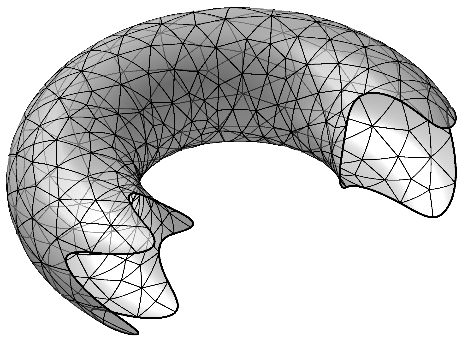
Figure 1: Mesh for the model problem using geometric interpolation order $k=3$ and meshsize $h=1/4$.

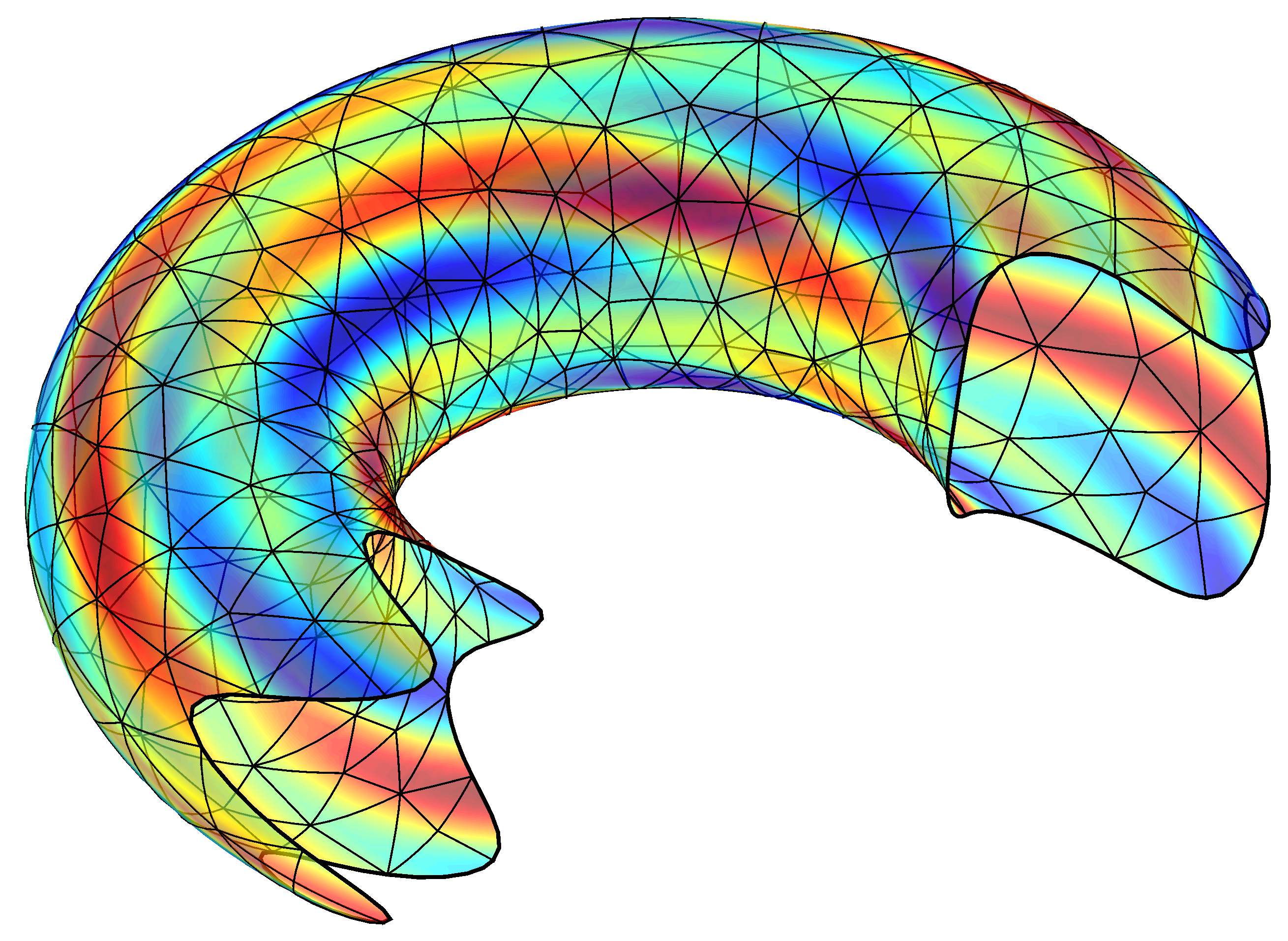
Figure 2: Numerical solution for the model problem using $k=3$ and meshsize $h=1/4$.

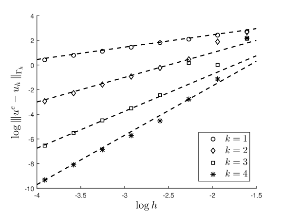
Figure 3: Convergence study of the model problem in energy norm with reference lines proportional to $h^{k}$. Note the instability in convergence rate for coarse meshes and higher order geometry approximation.

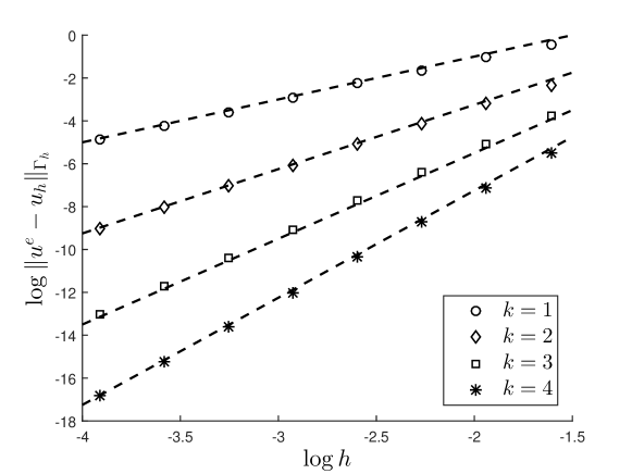
Figure 4: Convergence study of the model problem in $L^{2}$ norm with reference lines proportional to $h^{k+1}$.

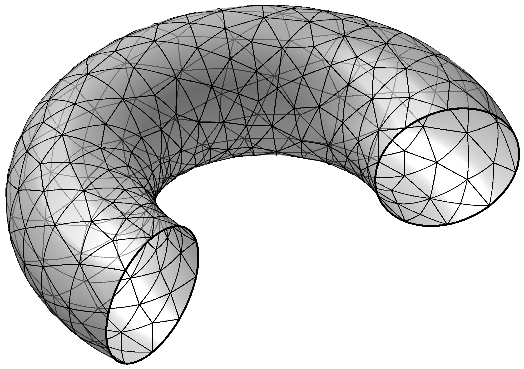
Figure 5: Mesh for a simplified version of the model problem ($N_{1}=N_{2}=0$) using geometric interpolation order $k=3$ and meshsize $h=1/4$. For this problem ${\Gamma_{h}^{l}}=\Gamma$, i.e. there is no boundary correction.

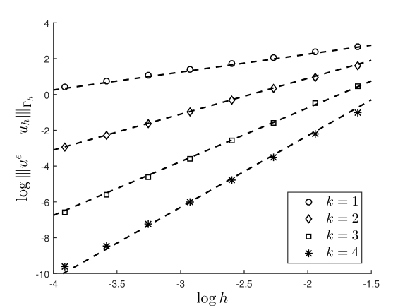
Figure 6: Convergence study for a simplified version of the model problem ($N_{1}=N_{2}=0$) in energy norm with reference lines proportional to $h^{k}$. Note that there is no instability in convergence rate for coarse meshes.

Acknowledgement.

This research was supported in part by EPSRC, UK, Grant No. EP/J002313/1, the Swedish Foundation for Strategic Research Grant No. AM13-0029, the Swedish Research Council Grants Nos. 2011-4992, 2013-4708, and Swedish strategic research programme eSSENCE.

References

• [1] P. F. Antonietti, A. Dedner, P. Madhavan, S. Stangalino, B. Stinner, and M. Verani. High order discontinuous Galerkin methods for elliptic problems on surfaces. SIAM J. Numer. Anal., 53(2):1145–1171, 2015.
• [2] J. H. Bramble, T. Dupont, and V. Thomée. Projection methods for Dirichlet’s problem in approximating polygonal domains with boundary-value corrections. Math. Comp., 26:869–879, 1972.
• [3] E. Burman, S. Claus, P. Hansbo, M. G. Larson, and A. Massing. CutFEM: Discretizing geometry and partial differential equations. Internat. J. Numer. Methods Engrg. (2015) , 2015.
• [4] E. Burman, P. Hansbo, and M. G. Larson. Technical Report arXiv:1507.03096, Department of Mathematics and Mathematical Statistics, Umeå University, Sweden, 2015.
• [5] E. Burman, P. Hansbo, and M. G. Larson. A stabilized cut finite element method for partial differential equations on surfaces: the Laplace-Beltrami operator. Comput. Methods Appl. Mech. Engrg., 285:188–207, 2015.
• [6] E. Burman, P. Hansbo, M. G. Larson, and A. Massing. A cut discontinuous Galerkin method for the Laplace-Beltrami operator. Technical Report arXiv::1507.05835, Department of Mathematics and Mathematical Statistics, Umeå University, Sweden, 2015.
• [7] E. Burman, P. Hansbo, M. G. Larson, and S. Zahedi. Cut finite element methods for coupled bulk–surface problems. Technical report, Department of Mathematics and Mathematical Statistics, Umeå University, Sweden, 2015.
• [8] P. G. Ciarlet. The finite element method for elliptic problems. North-Holland Publishing Co., Amsterdam-New York-Oxford, 1978. Studies in Mathematics and its Applications, Vol. 4.
• [9] A. Dedner, P. Madhavan, and B. Stinner. Analysis of the discontinuous Galerkin method for elliptic problems on surfaces. IMA J. Numer. Anal., 33(3):952–973, 2013.
• [10] A. Demlow. Higher-order finite element methods and pointwise error estimates for elliptic problems on surfaces. SIAM J. Numer. Anal., 47(2):805–827, 2009.
• [11] G. Dziuk. Finite elements for the Beltrami operator on arbitrary surfaces. In Partial differential equations and calculus of variations, volume 1357 of Lecture Notes in Math., pages 142–155. Springer, Berlin, 1988.
• [12] G. Dziuk and C. M. Elliott. Finite element methods for surface PDEs. Acta Numer., 22:289–396, 2013.
• [13] G. B. Folland. Introduction to partial differential equations. Princeton Universiy Press, second edition, 1995.
• [14] D. Gilbarg and N. S. Trudinger. Elliptic partial differential equations of second order. Classics in Mathematics. Springer-Verlag, Berlin, 2001. Reprint of the 1998 edition.
• [15] M. G. Larson and F. Bengzon. The finite element method: theory, implementation, and applications, volume 10 of Texts in Computational Science and Engineering. Springer, Heidelberg, 2013.
• [16] K. Larsson and M. G. Larson. A continuous/discontinuous Galerkin method and a priori error estimates for the biharmonic problem on surfaces. Technical Report arXiv:1305.2740v2, Department of Mathematics and Mathematical Statistics, Umeå University, Sweden, 2015.
• [17] J.-C. Nédélec. Curved finite element methods for the solution of integral singular equations on surfaces in ${\bf R}^{3}$. In Computing methods in applied sciences and engineering (Second Internat. Sympos., Versailles, 1975), Part 1, pages 374–390. Lecture Notes in Econom. and Math. Systems, Vol. 134. Springer, Berlin, 1976.
• [18] J. A. Nitsche. On Dirichlet problems using subspaces with nearly zero boundary conditions. In The mathematical foundations of the finite element method with applications to partial differential equations (Proc. Sympos., Univ. Maryland, Baltimore, Md., 1972), pages 603–627. Academic Press, New York, 1972.
• [19] M. A. Olshanskii, A. Reusken, and J. Grande. A finite element method for elliptic equations on surfaces. SIAM J. Numer. Anal., 47(5):3339–3358, 2009.
• [20] M. A. Olshanskii, A. Reusken, and X. Xu. A stabilized finite element method for advection-diffusion equations on surfaces. IMA J. Numer. Anal., 34(2):732–758, 2014.
• [21] Ridgway Scott. Interpolated boundary conditions in the finite element method. SIAM J. Numer. Anal., 12:404–427, 1975.
• [22] J. T. Wloka, B. Rowley, and B. Lawruk. Boundary value problems for elliptic systems. Cambridge University Press, Cambridge, 1995.