Measuring dark energy with the $E_{\rm iso}-E_{\rm p}$ correlation
of gamma-ray bursts using model-independent methods

We use two model-independent methods to standardize long gamma-ray bursts (GRBs) using the $E_{\rm iso}-E_{\rm p}$ correlation ($\log E_{\rm iso}=a+b\log E_{\rm p}$), where $E_{\rm iso}$ is the isotropic-equivalent gamma-ray energy and $E_{\rm p}$ is the spectral peak energy. We update 42 long GRBs and attempt to constrain the cosmological parameters. The full sample contains 151 long GRBs with redshifts from 0.0331 to 8.2. The first method is the simultaneous fitting method. We take the extrinsic scatter $\sigma_{\rm ext}$ into account and assign it to the parameter $E_{\rm iso}$. The best-fitting values are $a=49.15\pm 0.26$, $b=1.42\pm 0.11$, $\sigma_{\rm ext}=0.34\pm 0.03$ and $\Omega_{m}=0.79$ in the flat $\Lambda$CDM model. The constraint on $\Omega_{m}$ is $0.55<\Omega_{m}<1$ at the 1 $\sigma$ confidence level. If reduced $\chi^{2}$ method is used, the best-fit results are $a=48.96\pm 0.18$, $b=1.52\pm 0.08,$ and $\Omega_{m}=0.50\pm 0.12$. The second method uses type Ia supernovae (SNe Ia) to calibrate the $E_{\rm iso}-E_{\rm p}$ correlation. We calibrate 90 high-redshift GRBs in the redshift range from 1.44 to 8.1. The cosmological constraints from these 90 GRBs are $\Omega_{m}=0.23^{+0.06}_{-0.04}$ for flat $\Lambda$CDM and $\Omega_{m}=0.18\pm 0.11$ and $\Omega_{\Lambda}=0.46\pm 0.51$ for non-flat $\Lambda$CDM. For the combination of GRB and SNe Ia sample, we obtain $\Omega_{m}=0.271\pm 0.019$ and $h=0.701\pm 0.002$ for the flat $\Lambda$CDM and the non-flat $\Lambda$CDM, and the results are $\Omega_{m}=0.225\pm 0.044$, $\Omega_{\Lambda}=0.640\pm 0.082,$ and $h=0.698\pm 0.004$. These results from calibrated GRBs are consistent with that of SNe Ia. Meanwhile, the combined data can improve cosmological constraints significantly, compared to SNe Ia alone. Our results show that the $E_{\rm iso}-E_{\rm p}$ correlation is promising to probe the high-redshift universe.

1 Introduction

Gamma-ray bursts (GRBs) are the most violent explosions in the Universe, with the highest isotropic energy up to $10^{54}$ ergs (for reviews, see Mészáros 2006; Zhang 2007; Gehrels et al. 2009). Thus, they can be detected to the edge of the visible Universe (Ciardi & Loeb 2000; Lamb & Reichart 2000; Wang et al. 2012). For instance, the spectroscopically confirmed redshift of GRB090423 is about 8.2 (Tanvir et al. 2009; Salvaterra et al. 2009). Therefore, they are promising probes for the high-redshift Universe (for a recent review, see Wang et al. 2015). Many studies have been carried out to use GRBs for cosmological purposes, such as the star formation rate (Totani 1997; Wijers et al. 1998; Porciani & Madau 2001; Wang & Dai 2009, 2011a), the intergalactic medium metal enrichment (Barkana & Loeb 2004; Wang et al. 2012), dark energy (Dai, Liang & Xu 2004; Friedman & Bloom 2005; Schaefer 2007; Basilakos & Perivolaropoulos 2008; Wang, Qi & Dai 2011b), reionization (Totani et al. 2006; Gallerani et al. 2008; Wang 2013), possible anisotropic acceleration (Wang & Wang 2014a), and the two-point correlation (Li & Lin 2015).

To constrain the cosmological parameters, standard rulers or candles such as baryon acoustic oscillations (BAO; Cole et al. 2005; Eisenstein et al. 2005; Anderson et al. 2014), cosmic microwave background (CMB; Komatsu et al. 2011; Planck Collaboration 2013, 2015) and SNe Ia (Riess et al. 1998; Perlmutter et al. 1999; Suzuki et al. 2012) are required. The redshifts of BAO and SNe Ia are low, however, and the CMB is only a snapshot of cosmic expansion. Some parameters, such as the density and EOS parameter of dark energy (Wang 2012; Wang & Dai 2014; Wang & Wang 2014b), might evolve with redshift. GRBs can probe the evolution of these parameters at high redshifts and serve as complementary tools for SNe Ia. The study of these evolutions can differentiate dark energy models. Some luminosity correlations have been proposed to standardize GRBs (Amati et al. 2002; Ghirlanda et al. 2004a; Liang & Zhang 2005). Ghirlanda et al. (2004a) found a tight correlation between collimated energy $E_{\gamma}$ and the peak energy $E_{\rm p}$ of $\nu F_{\nu}$ spectrum. Dai, Liang & Xu (2004) used this correlation to constrain cosmological parameters with 12 GRBs. Liang & Zhang (2005) found the $E_{\rm iso}-E_{\rm p}-t_{\rm b}$ correlation and used this correlation to constrain cosmological parameters. Recently, Wang, Qi & Dai (2011b) constrained cosmological parameters with 109 GRBs using six GRB empirical correlations, and found $\Omega_{m}=0.31^{+0.13}_{-0.10}$ in the flat $\Lambda$CDM model. Other attempts have also been made to standardize GRBs (Ghirlanda et al. 2004b; Friedman & Bloom 2005; Schaefer 2007; Wang, Dai & Zhu 2007; Liang et al. 2008; Kodama et al. 2008; Qi, Lu & Wang 2009; Cardone et al. 2010; Wang & Dai 2011c). These methods of standardizing the long GRBs are mainly based on some empirical correlations, such as the $E_{\rm iso}-E_{\rm p}$ (Amati et al. 2002), $E_{\rm p}-L_{\rm p}$ (Schaefer 2003; Wei & Gao 2003), and $E_{\rm p}-E_{\gamma}$ (Ghirlanda et al. 2004a), where $L_{\rm p}$ is the peak luminosity, $E_{\rm p}$ is the peak energy in cosmological rest frame, $E_{\rm iso}$ is the isotropic-equivalent energy, and $E_{\gamma}$ is the collimation-corrected energy. Correlations within X-ray afterglow light curves have also been studied (Dainotti, Cardone & Capozziello 2008; Dainotti et al. 2010; Qi & Lu 2010).

In this paper, we focus on the usage of the $E_{\rm iso}-E_{\rm p}$ correlation. Amati et al. (2002) discovered this correlation with a small sample of $Beppo$SAX GRBs. Since many more GRBs are detected, attempts have been made to use this correlation for the purpose of cosmology. Amati et al. (2008) used a simultaneous fitting method to constrain the $E_{\rm iso}-E_{\rm p}$ correlation coefficients and cosmological parameters together with 70 long GRBs. The extrinsic scatter $\sigma_{\rm ext}$ was taken into consideration in this method (D’Agostini 2005). Amati et al. (2008) assigned $\sigma_{\rm ext}$ to $E_{\rm p}$ and found $0.04<\Omega_{m}<0.40$ and $\sigma_{\rm ext}=0.17\pm 0.02$ at 1 $\sigma$ confidence level in the flat $\Lambda$CDM universe. For non-flat $\Lambda$CDM model, the results are $\Omega_{m}\in[0.04,0.40]$ and $\Omega_{\Lambda}<1.05$ (Amati et al. 2008). However, Ghirlanda (2009) doubted this result. He claimed that the extrinsic scatter term should be assigned to $E_{\rm iso}$. This is consistent with D’Agostini (2005), who described that the extrinsic scatter $\sigma_{\rm ext}$ should be assigned to the parameter that also depends on hidden variables (cosmological parameters in our study). We discuss this point in detail in Sect. 3.1. However, this would lead to no constraint on cosmological parameters with the same 70 GRBs from Amati et al. (2008). We test it again with a larger sample in this paper.

The calibration method is also helpful to standardize GRBs. Imitating the example of standardizing the standard candle of SNe Ia with Cepheid variables, GRBs can also be calibrated with SNe Ia (Liang et al. 2008; Kodama et al. 2008; Wei 2010; Lin, Li, & Change 2015). This method is also cosmological model independent. Liang et al. (2008) calibrated 42 high redshift GRBs with SNe Ia. Five interpolation methods were used and the results were consistent with each other. Wei (2010) standardized 59 high-redshift GRBs with SNe Ia, using the $E_{\rm iso}-E_{\rm p}$ correlation, and found that GRBs can improve the constraint on cosmological parameters. Wang & Dai (2011c) calibrated 116 GRBs with Union 2 SNe Ia with cosmographic parameters.

We use 151 GRBs, 109 of which are taken from Amati et al. (2008) and Amati, Frontera & Guidorzi (2009). The remaining 42 GRBs are the updated long GRBs, which were detected by Fermi GBM, Konus-Wind, Swift-BAT, and Suzaku-WAM. The energy band, fluence, low ($\alpha$), high ($\beta$) energy photon indices, spectral peak energy, and redshift are taken from the refined analysis of the corresponding GRB team. We test whether this larger GRB sample can help to constrain cosmological models better. First, we constrain the cosmological parameters and coefficients of the $E_{\rm iso}-E_{\rm p}$ correlation simultaneously. Then, we calibrate these GRBs with SNe Ia using the $E_{\rm iso}-E_{\rm p}$ correlation. At last, we compare these two methods and discuss them.

This paper is organized as follows. In the next section, we introduce the GRBs data and perform the K-correction. In Sect. 3, we test whether the redshift evolution of the $E_{\rm iso}-E_{\rm p}$ correlation is significant, and use a simultaneous fitting method to constrain cosmological parameters and coefficients of the $E_{\rm iso}-E_{\rm p}$ correlation. In Sect. 4, we use SNe Ia to calibrate the $E_{\rm iso}-E_{\rm p}$ correlation, then we use these calibrated GRBs to constrain cosmological parameters. Summary and discussions are given in Sect. 5.

2 Updated GRB sample

We collect all GRBs with information of redshift, fluence, peak energy, and photon indices from GCN Circulars Archive Cucchiara et al. (2011) and Gendre et al. (2013) until February 13, 2014. The updated sample contains 42 updated long GRBs. We list these GRBs in Table LABEL:sample. The spectra of these GRBs are obtained from the refined analysis of Fermi GBM team, Konus-Wind team, Swift-BAT team, and Suzaku-WAM team. The redshifts extend from 0.34 to 5.91. The spectrum is modeled by a broken power law (Band et al. 1993),

$$\Phi(E)=\left\{\begin{array}[]{ll}AE^{\alpha}{\rm e}^{-(2+\alpha)E/E_{\rm p,obs}}&E\leq\frac{\alpha-\beta}{2+\alpha}E_{\rm p,obs}\\ \nobreak\leavevmode&\nobreak\leavevmode\\ BE^{\beta}&{\rm otherwise,}\end{array}\right.\$$ (1)

where $E_{\rm p,obs}$ is the observed peak energy, $\alpha$ and $\beta$ are the low and high energy photon indices, respectively. We take the typical spectral index values for those GRB whose indices are not given out in the references, i.e., $\alpha=-1.0$ and $\beta=-2.2$ (Salvaterra et al. 2009).

With these spectra parameters, we can obtain the peak energy in the cosmological rest frame by $E_{\rm p}=E_{\rm p,obs}\times(1+z)$ and the bolometric fluence in the band of $1-10^{4}$ keV by (Bloom, Frail & Sari 2001)

$$S_{\rm bolo}=S\ {\times}\ \frac{\int_{1/(1+z)}^{10^{4}/(1+z)}{E\Phi(E)dE}}{\int_{E_{\rm min}}^{E_{\rm max}}{E\Phi(E)dE}}\ ,$$ (2)

where $S$ is the observed fluence, $E_{\rm min}$ and $E_{\rm max}$ are the detection limits of the instrument, and $z$ is the redshift.

In the $E_{\rm iso}-E_{\rm p}$ plane, $E_{\rm p}$ is an observed value, which is not dependent on the cosmological model. However, $E_{\rm iso}$ depends on the cosmological model from

$$E_{\rm iso}=4\pi d_{\rm L}^{2}S_{\rm bolo}(1+z)^{-1},$$ (3)

where $d_{\rm L}$ is the luminosity distance. Assuming a flat $\Lambda$CDM model, the $d_{\rm L}$ can be expressed with Hubble expansion rate

$$d_{\rm L}(\Omega_{m},z)=(1+z)\frac{c}{H_{0}}\int_{0}^{z}\frac{dz^{\prime}}{\sqrt{\Omega_{m}(1+z)^{3}+1-\Omega_{m}}},$$ (4)

where $\Omega_{m}$ is the matter density at present, and $H_{0}$ is the Hubble constant. Since the Hubble constant is precisely measured, we take $H_{0}=67.8$ km s^-1 Mpc^-1 (Planck Collaboration 2013, 2015), except when we use the combination data of SNe and GRB to constrain cosmological models.

We list 42 updated GRBs in Table LABEL:sample. The isotropic energy $E_{\rm iso}$ is calculated with benchmark parameters with $\Omega_{m}=0.308$ for the flat $\Lambda$CDM universe (Planck Collaboration 2013, 2015). During the calculation, we only take the errors propagating from the spectrum parameters, namely observed fluence $S$ and peak energy $E_{\rm p,obs}$. The uncertainties from other parameters are attributed into the extrinsic scatter $\sigma_{\rm ext}$.

3 The $E_{\rm iso}-E_{\rm p}$ correlation and constraints on cosmological parameters

3.1 The $E_{\rm iso}-E_{\rm p}$ correlation

To constrain cosmological models more precisely, we combine our updated 42 GRBs with 109 GRBs from Amati et al. (2008) and Amati, Frontera & Guidorzi (2009). The full sample contains 151 GRBs and covers the redshift range from 0.0331 to 8.2. We parameterize the $E_{\rm iso}-E_{\rm p}$ correlation as follows:

$$\log\frac{E_{\rm iso}}{\text{erg}}=a+b\leavevmode\nobreak\ \log\frac{E_{\rm p}}{\text{keV}},$$ (5)

where $a$ and $b$ are the intercept and slope. Here $E_{\rm p}$ has been corrected into the cosmological rest frame.

Before constraining cosmological models, we test the possible redshift evolution of the $E_{\rm iso}-E_{\rm p}$ correlation using the maximum likelihood method. The full data is divided into four redshift bins: $[0.0331,0.958]$, $[0.966,1.613]$, $[1.619,2.671],$ and $[2.69,8.2]$. Each bin almost includes the same number of GRBs. The results are shown in Table 2. We give out the best-fit values and 1 $\sigma$ uncertainties in the coefficients $a$, $b,$ and the extrinsic scatter $\sigma_{\rm ext}$. The $\sigma_{\rm ext}$ is almost constant in different bins. Its value is about 0.34, which implies that the extrinsic scatter dominates the error size. The results show no statistically significant evidence for the redshift evolution of the $E_{\rm iso}-E_{\rm p}$ correlation. This result is consistent with those of Basilakos & Perivolaropoulos (2008) and Wang, Qi & Dai (2011b). The full data result are also shown in Figure 1. This result illustrates that the $E_{\rm iso}-E_{\rm p}$ correlation fits the data well.

As discussed by D’Agostini (2005), we use the following likelihood to fit the linear relation $y=a+bx$,

$$\mathcal{L}(\Omega_{m},a,b,\sigma_{\rm ext})\propto\prod\limits_{i}{\frac{1}{{\sqrt{\sigma^{2}_{ext}+\sigma^{2}_{y_{i}}+b^{2}\sigma^{2}_{x_{i}}}}}}\;$$

$$\times\exp\left[-\frac{{(y_{i}-a-bx_{i})^{2}}}{{2(\sigma^{2}_{ext}+\sigma^{2}_{y_{i}}+b^{2}\sigma^{2}_{x_{i}})}}\right].$$ (6)

Following the description of D’Agostini (2005), the parameter $y$ should not only depend on $x$, but also depend on some hidden variables ($\Omega_{m}$ here). Thus, the expression of the $E_{\rm iso}-E_{\rm p}$ plane should be written as $y=\log\frac{E_{\rm iso}}{\text{erg}}$ and $x=\log\frac{E_{\rm p}}{\text{keV}}$. However, Amati et al. (2008) set $y=\log\frac{E_{\rm p}}{\text{keV}}$, thus the extrinsic scatter $\sigma_{\rm ext}$ does not contain the error from the cosmological models.

Figure 1: The $E_{\rm iso}-E_{\rm p}$ correlation. The solid black, dotted, and dashed lines represent the best-fit line, $1\,\sigma_{\rm ext}$ region, and $2\,\sigma_{\rm ext}$ region, respectively.

3.2 Simultaneous fitting

Since the $E_{\rm iso}-E_{\rm p}$ correlation does not evolve with redshift, it can be used to constrain parameters directly. We emphasize that there is no circularity problem in the simultaneous fitting method because we do not assume any cosmological model. In this section, we focus on the constraint on the flat $\Lambda$CDM model. The luminosity distance is expressed as Eq. (4).

Using the likelihood expressed in equation (3.1), we can constrain the current matter density $\Omega_{m}$, the extrinsic scatter parameter $\sigma_{\rm ext}$, and the coefficients of the $E_{\rm iso}-E_{\rm p}$ correlation simultaneously. In our calculations, the best-fit values are $a=49.15\pm 0.26$, $b=1.42\pm 0.12$, $\sigma_{\rm ext}=0.34\pm 0.03,$ and $\Omega_{m}=0.76$. We show the constraint on $\Omega_{m}$ in Fig. 2 with a solid line. The 1 $\sigma$ uncertainty is $\Omega_{m}\in[0.55,1]$. We also use the reduced $\chi^{2}$ method to constrain the matter density. This method also includes the effect of extrinsic scatter

$$\chi^{2}=\sum_{i}{(y_{i}-a-bx_{i})^{2}/(\sigma^{2}_{y_{i}}+b^{2}\sigma^{2}_{x_{i}}+\sigma^{2}_{\rm ext})}.$$ (7)

The hidden variables (cosmological parameters) are included in $E_{\rm iso}$. The extrinsic scatter is used to set the reduced $\chi^{2}$ to unity, which is also used in SNe Ia cosmology(Suzuki et al. 2012). The value of $\sigma_{\rm ext}$ is 0.34 when the reduced $\chi^{2}$ is unity. The best-fit results are $a=48.96\pm 0.18$, $b=1.52\pm 0.08,$ and $\Omega_{m}=0.50\pm 0.12$. The constraint from reduced $\chi^{2}$ method is roughly consistent with the likelihood method. The $\chi^{2}/\chi^{2}_{\rm min}$ evolution with $\Omega_{m}$ are shown in Fig.  2 with a dashed line. If the extrinsic scatter is not considered, the results are $a=48.50\pm 0.05$, $b=1.81\pm 0.02,$ and $\Omega_{m}=0.19\pm 0.05$.

There is a mild tension between the results from the likelihood method and the reduced $\chi^{2}$ method. The extrinsic scatter is large, which loosely constrains the cosmological parameters. When we calculate the parameter $E_{\rm iso}$, a cosmological model and a spectrum model are used, while the uncertainties from them are not well established, thus we take these uncertainties into a scatter parameter $\sigma_{\rm ext}$. This scatter should be assigned to the parameter $E_{\rm iso}$. In the future, this scatter can be reduced, since precise observation and data analysis will be performed by the team of Sino-French space-based multiband astronomical variable objects monitor (SVOM; Basa et al. 2008; Götz et al. 2009; Paul et al. 2011).

We also compare our results to the current precise measurements, such as the results from $Planck$+WMAP (Planck Collaboration 2013), BAO (Beutler et al. 2011; Anderson et al. 2014; Kazin et al. 2014; Ross et al. 2015), and SNe Ia (Conley et al. 2011; Suzuki et al. 2012). We show them in Table 3. The best-fit $\Omega_{m}$ by GRBs, using $\chi^{2}$ method, conflicts with the observation of CMB and BAO. For the results from SNe Ia, however, if both statistical and systematic errors are included, the constraints on cosmological parameters are loose(Kowalski et al. 2008; Amanullah et al. 2010; Suzuki et al. 2012). In this case, the best-fit $\Omega_{m}$ with GRBs, using $\chi^{2}$ method, is consistent with those from SNe Ia at $1\sigma$ confidence level; see Fig. 12 of Kowalski et al. (2008), Fig. 10 of Amanullah et al. (2010) and Fig. 5 of Suzuki et al. (2012).

Figure 2: The evolution of $\log(\mathcal{L})/\log(\mathcal{L})_{\rm min}$ as a function of $\Omega_{m}$ in the flat $\Lambda$CDM universe is shown with solid line from maximum likelihood method. The dashed line is the $\chi^{2}/\chi^{2}_{\rm min}-\Omega_{m}$ plot from reduced $\chi^{2}$ method. The dotted line is obtained with the 90 GRBs calibrated on the SNe Ia (see section 4).

4 Calibration of the $E_{\rm iso}-E_{\rm p}$ correlation

4.1 Standardizing GRBs with SNe Ia

Just as using Cepheid variables to standardize SNe Ia, the GRBs can be calibrated with SNe Ia. We can use the calibrating method to standardize the GRBs with the $E_{\rm iso}-E_{\rm p}$ correlation. With this approach, the parameters $a$ and $b$ are obtained and only cosmological parameters remain free. We use the latest Union 2.1 data from Suzuki et al. (2012). This method is also cosmological model independent (Liang et al. 2008; Kodama et al. 2008; Wei 2010). The extrinsic scatter is also be taken into account when calculating the error propagation of $E_{\rm iso}$. The full GRB data is separated into two groups. The dividing line is the highest redshift in SNe Ia Union 2.1 data, namely, $z=1.414$. The low-redshift group ($z<1.414$) includes 61 GRBs and the high-redshift group ($z>1.414$) contains 90 GRBs.

Firstly, the linear interpolation method is used to calibrate the distance moduli $\mu$ of 61 low-redshift GRBs. Liang et al. (2008) have shown that there are no differences on the final result between the linear interpolation and the cubic interpolation. The 1 $\sigma$ error of the distance moduli $\sigma_{\mu,i}$ can be obtained as follows:

$$\sigma_{\mu}^{2}=(\frac{z_{i+1}-z}{z_{i+1}-z_{i}})^{2}\epsilon_{\mu,i}^{2}+(\frac{z-z_{i}}{z_{i+1}-z_{i}})^{2}\epsilon_{\mu,i+1}^{2},$$ (8)

where $z_{i+1}$ and $z_{i}$ are the redshift of the two nearest SNe Ia and $\epsilon_{\mu,i+1}$ and $\epsilon_{\mu,i}$ are the errors of these two SNe Ia. The redshift of interpolated GRB lies between $z_{i}$ and $z_{i+1}$.

After the distance moduli of 61 low-redshift GRBs are obtained, the luminosity distance can be derived from

$$\mu=5\log\frac{d_{\rm L}}{\text{Mpc}}+25.$$ (9)

Then the isotropic-equivalent energy $E_{\rm iso}$ can be calculated from Eq. (3). Following Schaefer (2007) and Liang et al. (2008), we use the bisector of the two ordinary least squares method (Isobe et al. 1990) to fit the $E_{\rm iso}-E_{\rm p}$ correlation. The best-fit values are $a=48.46\pm 0.033$ and $b=1.766\pm 0.007$. The result is shown in Fig. 3. The errors of distance moduli are not taken into consideration because the extrinsic scatter $\sigma_{\rm ext}$ dominates the error size in the regression analysis (Schaefer 2007). Thus, we take $\sigma_{\rm ext}$ directly into account during the calculations of the uncertainties of high-redshift GRBs ($\sigma_{\log E_{\rm iso}}$). From the previous section, the value of $\sigma_{\rm ext}$ is nearly constant, so we typically set $\sigma_{\rm ext}=0.34$.

Figure 3: Low-redshift GRM sample $E_{\rm iso}-E_{\rm p}$ correlation. Black line is the best-fit result obtained by using the bisector of the two ordinary least squares method. The dotted line represents the $1\,\sigma_{\rm ext}$ region and dashed line the $2\,\sigma_{\rm ext}$ region.

We have shown that the $E_{\rm iso}-E_{\rm p}$ correlation does not evolve with redshift in the previous section. Thus, the calibrated $E_{\rm iso}-E_{\rm p}$ correlation can be extrapolated to the high-redshift sample, namely, $z>1.414$ group. Using Eq. (5), we can derive $E_{\rm iso}$ of high-redshift GRBs. The propagated uncertainties of $E_{\rm iso}$ can be calculated from

$$\sigma_{\log E_{\rm iso}}^{2}=\sigma_{a}^{2}+\left(\sigma_{b}\log\frac{E_{\rm p}}{\text{keV}}\right)^{2}+\left(\frac{b}{\ln 10}\,\frac{\sigma_{E_{\rm p}}}{E_{\rm p}}\right)^{2}+\sigma_{\rm ext}^{2},$$ (10)

where the value of $\sigma_{\rm ext}$ is 0.34. The values of $\sigma_{a}$ and $\sigma_{b}$ are derived from the bisector of the two ordinary least squares method.

Then, we use Eq. (3) and Eq. (9) to derive the distance moduli. The propagated uncertainty is given by the following equation:

$$\sigma_{\mu}=\left[\left(\frac{5}{2}\sigma_{\log E_{\rm iso}}\right)^{2}+\left(\frac{5}{2\ln 10}\,\frac{\sigma_{S_{\rm bolo}}}{S_{\rm bolo}}\right)^{2}\right]^{1/2}.$$ (11)

The calibrated 90 high-redshift GRBs are listed in Table LABEL:calibratedGRB. This sample can be used to constrain cosmological models directly. Compared with Wei (2010), the error bars of distance moduli of our results are smaller. The main reason is that we use a larger sample, which leads to a smaller $\sigma_{\rm ext}$. The extrinsic scatter parameter has been taken into consideration during the calculation of the error size of $E_{\rm iso}$.

4.2 Constraining cosmological models

These GRBs carry the information of high-redshift universe, and can be taken as good complements to the Union 2.1 data set. We test if these high-redshift GRBs alone can constrain the $\Lambda$CDM model. Using the distance modulus in Eq. (4) and Eq. (9), the $\chi^{2}$ is

$$\chi^{2}_{\text{GRB}}({\Omega_{m}})=\sum\limits_{i=1}^{90}\frac{\left[\mu_{\rm cal}(z_{i})-\mu(z_{i})\right]^{2}}{\sigma^{2}(z_{i})}\,,$$ (12)

where $\mu_{\rm cal}$ is the calibrated GRB distance modulus listed in Table LABEL:calibratedGRB. The best-fit result is $\Omega_{m}=0.23^{+0.06}_{-0.04}$ with 1 $\sigma$ uncertainty. The $\chi^{2}$ evolution with $\Omega_{m}$ is shown in Fig.  2. This result is consistent with the constraints from SNe Ia (Conley et al. 2011; Suzuki et al. 2012), CMB (Planck Collaboration 2013, 2015), and BAO (Beutler et al. 2011; Anderson et al. 2014; Kazin et al. 2014; Ross et al. 2015) at 1 $\sigma$ confidence level, as shown in Table  3.

Since this GRB sample can constrain cosmological parameters successfully, we also combine the calibrated GRB data with SNe Ia from Union 2.1 sample to constrain cosmological models. For the flat $\Lambda$CDM, we obtain $\Omega_{m}=0.271\pm 0.019$ and $h=0.701\pm 0.002$, where $h$ is the Hubble constant in units of 100 km s^-1 Mpc^-1. This is very consistent with the Union 2.1 SNe Ia data. For the non-flat $\Lambda$CDM, the luminosity distance is different and can be expressed as follows:

$$d_{L}=\left\{\begin{array}[]{l}\displaystyle cH_{0}^{-1}(1+z)(-\Omega_{k})^{-1/2}\sin[(-\Omega_{k})^{1/2}I],\leavevmode\nobreak\ \Omega_{k}<0,\\ \displaystyle cH_{0}^{-1}(1+z)I,\leavevmode\nobreak\ \leavevmode\nobreak\ \leavevmode\nobreak\ \leavevmode\nobreak\ \leavevmode\nobreak\ \leavevmode\nobreak\ \leavevmode\nobreak\ \leavevmode\nobreak\ \leavevmode\nobreak\ \leavevmode\nobreak\ \leavevmode\nobreak\ \leavevmode\nobreak\ \leavevmode\nobreak\ \leavevmode\nobreak\ \leavevmode\nobreak\ \leavevmode\nobreak\ \leavevmode\nobreak\ \leavevmode\nobreak\ \leavevmode\nobreak\ \leavevmode\nobreak\ \leavevmode\nobreak\ \leavevmode\nobreak\ \leavevmode\nobreak\ \leavevmode\nobreak\ \leavevmode\nobreak\ \leavevmode\nobreak\ \leavevmode\nobreak\ \leavevmode\nobreak\ \leavevmode\nobreak\ \leavevmode\nobreak\ \leavevmode\nobreak\ \leavevmode\nobreak\ \leavevmode\nobreak\ \leavevmode\nobreak\ \leavevmode\nobreak\ \leavevmode\nobreak\ \leavevmode\nobreak\ \leavevmode\nobreak\ \leavevmode\nobreak\ \leavevmode\nobreak\ \leavevmode\nobreak\ \Omega_{k}=0,\\ \displaystyle cH_{0}^{-1}(1+z)\Omega_{k}^{-1/2}\sinh[\Omega_{k}^{1/2}I],\leavevmode\nobreak\ \leavevmode\nobreak\ \leavevmode\nobreak\ \leavevmode\nobreak\ \leavevmode\nobreak\ \leavevmode\nobreak\ \leavevmode\nobreak\ \leavevmode\nobreak\ \leavevmode\nobreak\ \leavevmode\nobreak\ \leavevmode\nobreak\ \leavevmode\nobreak\ \leavevmode\nobreak\ \leavevmode\nobreak\ \,\Omega_{k}>0,\\ \end{array}\right.$$ (13)

where

$$\Omega_{k}=1-\Omega_{m}-\Omega_{\Lambda},$$ (14)

and

$$I=\int_{0}^{z}\frac{dz}{\sqrt{(1+z)^{3}\Omega_{m}+\Omega_{\Lambda}+(1+z)^{2}\Omega_{k}}}.$$ (15)

The $\chi^{2}$ of SNe Ia is constructed as follows:

$$\chi^{2}_{\text{SNe}}({h,\Omega_{m},\Omega_{\Lambda}})=\sum\limits_{i=1}^{580}\frac{\left[\mu_{\rm obs}(z_{i})-\mu(z_{i})\right]^{2}}{\sigma^{2}(z_{i})}.$$ (16)

Then the total $\chi^{2}$ is

$$\chi^{2}_{\text{total}}({h,\Omega_{m},\Omega_{\Lambda}})=\chi^{2}_{\text{SNe}}({h,\Omega_{m},\Omega_{\Lambda}})+\chi^{2}_{\text{GRB}}({h,\Omega_{m},\Omega_{\Lambda}}).$$ (17)

The best-fit values with 1 $\sigma$ uncertainties are $\Omega_{m}=0.225\pm 0.044$, $\Omega_{\Lambda}=0.640\pm 0.082,$ and $h=0.698\pm 0.004$ for the combined sample (SNe+GRB). For the GRB sample, we obtain $\Omega_{m}=0.18\pm 0.11$ and $\Omega_{\Lambda}=0.46\pm 0.51$, which is consistent with the SNe Ia results at 1 $\sigma$ confidence level. The combined sample can help to constrain cosmological parameters much tighter because not only is the sample enlarged, but also the redshift covers a much wider. The flatness of the Universe depends on the curvature parameter, that is to say, $\Omega_{k}=1-\Omega_{\Lambda}-\Omega_{m}$. In Fig. 4, we use three samples, GRB, SNe, and combination of GRB+SNe to constrain the cosmological model. Both results prefer a flat universe at the 1 $\sigma$ confidence level. The constraint from the GRB is almost perpendicular to that from SNe Ia in the $\Omega_{m}-\Omega_{\Lambda}$ plane. Thus GRBs can significantly help to constrain $\Omega_{m}$ because, in this redshift domain, the dark matter dominates the evolution of the Universe. We also show constraints on $\Omega_{m}-h$ in Fig. 5, and $\Omega_{\Lambda}-h$ in Fig.  6.

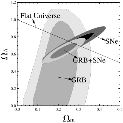
Figure 4: 1 $\sigma$ and 2$\sigma$ constraints on $\Omega_{m}$ and $\Omega_{\Lambda}$. We use three samples and plot them into different colors. The solid line shows the $\Omega_{k}=0$ case.

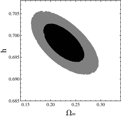
Figure 5: 1 $\sigma$ and 2$\sigma$ constraints on $\Omega_{m}$ and $h$ from SNe Ia and GRB data.

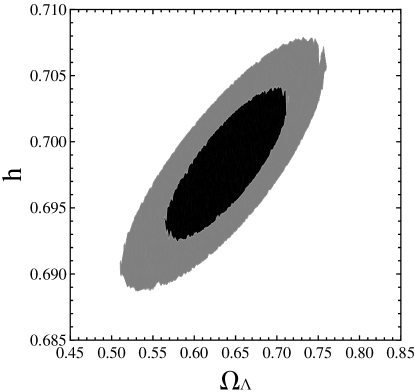
Figure 6: 1 $\sigma$ and 2$\sigma$ constraints on the $\Omega_{\Lambda}$ and $h$ from SNe Ia and GRB data.

5 Discussions and summary

In this paper, we update 42 long GRBs for the $E_{\rm iso}-E_{\rm p}$ correlation and combine them with 109 long GRBs from Amati et al. (2008) and Amati, Frontera & Guidorzi (2009). This sample contains GRBs detected by different detectors with different sensitivities. Thus, the sample might be biased, but this bias should only have a weak effect on our results. We also use the complete sample to perform our analysis. We use the same criteria as Salvaterra et al. (2012) and Pescalli et al. (2015) to collect GRBs. The results are $a=49.45\pm 0.61$, $b=1.24\pm 0.22$ and $\sigma_{\rm ext}=0.38\pm 0.06$, while no constraint on $\Omega_{m}$ is found. These results are in tension with that of our updated full sample with a larger extrinsic scatter. No statistical evidence for the redshift evolution of the $E_{\rm iso}-E_{\rm p}$ is found in the full sample.

For cosmological purposes, we fit the $E_{\rm iso}-E_{\rm p}$ plane and the cosmological parameters simultaneously. Using a likelihood function we obtain $a=49.15\pm 0.26$, $b=1.42\pm 0.11$, $\sigma_{\rm ext}=0.34\pm 0.03,$ and $\Omega_{m}\in[0.55,1]$. Using the reduced $\chi^{2}$, we obtain $a=48.96\pm 0.18$, $b=1.52\pm 0.08,$ and $\Omega_{m}=0.50\pm 0.12$. The results from these two fitting methods are in mild tension. The main reason is that the extrinsic scatter of this correlation is too large. Thus, Ghirlanda (2009) finds no constraint with a smaller sample using the likelihood method. We also use a calibrating method. Based on the SNe Ia data, we obtain 90 calibrated GRBs. From these calibrated GRBs, we acquire $\Omega_{m}=0.23^{+0.06}_{-0.04}$ for flat $\Lambda$CDM and for the non-flat $\Lambda$CDM, we obtain $\Omega_{m}=0.18\pm 0.11$ and $\Omega_{\Lambda}=0.46\pm 0.51$. We also combine the GRB sample with SNe Ia Union 2.1 data and obtain $\Omega_{m}=0.271\pm 0.019$ and $h=0.701\pm 0.002$ for the flat $\Lambda$CDM. For the non-flat $\Lambda$CDM, the results are $\Omega_{m}=0.225\pm 0.044$, $\Omega_{\Lambda}=0.640\pm 0.082,$ and $h=0.698\pm 0.004$. We list our results in Table 3, and compare them with the results from other current measurements. The results from GRBs are consistent with results from SNe Ia in 1 $\sigma$ confidence level (Conley et al. 2011; Suzuki et al. 2012), while they conflict with CMB (Planck Collaboration 2013, 2015) and BAO (Beutler et al. 2011; Anderson et al. 2014; Kazin et al. 2014; Ross et al. 2015). We also found that the GRBs can help to constrain dark matter better. The constraint from GRB are almost perpendicular to that from SNe Ia in the $\Omega_{m}-\Omega_{\Lambda}$ plane. The main reason might be that at high redshift, the dark matter dominates the Universe.

The extrinsic scatter is taken into account in both the simultaneous fitting method and the calibrating method. Our results shows that tighter constraints on cosmological model can be obtained with the calibrating method. For the simultaneous fitting method, the reduced $\chi^{2}$ method gives a more stringent constraint on cosmological parameters than the likelihood method, but the constraint is still loose because of the large extrinsic scatter. This scatter is introduced by both cosmological models and the GRB spectrum parameters, such as $E_{\rm p}$, fluence, and photon index. The spectrum parameters can be precisely measured by SVOM (Basa et al. 2008; Götz et al. 2009; Paul et al. 2011), which can reduce the extrinsic scatter. The GRBs from SVOM would better help shed light on the properties of early Universe.

Table 1: 42 updated long GRBs. (a) $E_{\rm iso}$ is computed with benchmark parameters: $H_{0}=67.8$ km s^-1 Mpc^-1 and $\Omega_{m}=0.308$; (b) Instruments: FG=Fermi GBM, KW=Konus-Wind, SB= Swift-BAT and SW=Suzaku-WAM; (c) References for the spectrum parameters: (1) Sugita et al. (2010); (2) Golenetskii et al. (2010a); (3) Golenetskii et al. (2010b); (4) von Kienlin et al. (2010); (5) Golenetskii et al. (2010c); (6) Golenetskii et al. (2010d); (7) Cucchiara et al. (2011); (8) Golenetskii et al. (2011a); (9) Golenetskii et al. (2011b); (10) Golenetskii et al. (2011c); (11) Golenetskii et al. (2011d); (12) Golenetskii et al. (2011e); (13) Xiong et al. (2011); (14) Golenetskii et al. (2011f); (15) Pelassa et al. (2011); (16) Golenetskii et al. (2011g); (17) Golenetskii et al. (2012a); (18) Collazzi et al. (2012); (19) Krimm et al. (2012a); (20) Stamatikos et al. (2012); (21) Krimm et al. (2012b); (22) Golenetskii et al. (2012b); (23) Krimm et al. (2012c); (24) Golenetskii et al. (2013a) (25) Younes et al. (2013); (26) Golenetskii et al. (2013b); (27) Xiong et al. (2013a); (28) von Kienlin et al. (2013); (29) Golenetskii et al. (2013c); (30) Palshin et al. (2013); (31) Xiong et al. (2013b); (32) Golenetskii et al. (2013d) (33) Fitzpatrick et al. (2013a); (34) Fitzpatrick et al. (2013b); (35) Golenetskii et al. (2013e); (36) Golenetskii et al. (2013f) (37) Golenetskii et al. (2013g); (38) Golenetskii et al. (2013h); (39) Fitzpatrick et al. (2013c); (40) Krimm et al. (2013); (41) von Kienlin et al. (2014); (42) Zhang (2014).

GRB	Redshift	$S_{\rm bolo}$($10^{-5}$ erg cm-2)	$E_{\rm p}$(keV)	$E_{\rm iso}^{(a)}$($10^{53}$ erg)	Instruments(b)	Refs. for spectrum(c)
100413	3.90	$2.36\pm 0.77$	$1783.60\pm 374.85$	$7.31\pm 4.56$	SW	(1)
100621	0.54	$5.75\pm 0.64$	$146.49\pm 23.90$	$0.46\pm 0.20$	KW	(2)
100704	3.60	$0.70\pm 0.07$	$809.60\pm 135.70$	$1.91\pm 0.61$	KW	(3)
100728B	2.45	$0.29\pm 0.01$	$359.11\pm 48.34$	$0.42\pm 0.12$	FG	(4)
100814	1.44	$1.39\pm 0.23$	$312.32\pm 48.80$	$0.77\pm 0.31$	KW	(5)
100906	1.73	$3.56\pm 0.55$	$387.23\pm 244.07$	$2.77\pm 1.18$	KW	(6)
110205	2.22	$3.32\pm 0.68$	$740.60\pm 322.00$	$4.04\pm 1.82$	KW/SB/SW	(7)
110213	1.46	$1.55\pm 0.23$	$223.86\pm 70.11$	$0.88\pm 0.41$	KW	(8)
110422	1.77	$9.32\pm 0.02$	$421.04\pm 13.85$	$7.58\pm 1.67$	KW	(9)
110503	1.61	$2.76\pm 0.21$	$572.25\pm 50.95$	$1.89\pm 0.55$	KW	(10)
110715	0.82	$2.73\pm 0.24$	$218.40\pm 20.93$	$0.51\pm 0.16$	KW	(11)
110731	2.83	$2.51\pm 0.01$	$1164.32\pm 49.79$	$4.62\pm 1.06$	KW	(12)
110818	3.36	$1.05\pm 0.08$	$1117.47\pm 241.11$	$2.56\pm 0.85$	FG	(13)
111008	5.00	$1.06\pm 0.11$	$894.00\pm 240.00$	$4.82\pm 1.61$	KW	(14)
111107	2.89	$0.18\pm 0.03$	$420.44\pm 124.58$	$0.34\pm 0.14$	FG	(15)
111209	0.68	$69.47\pm 8.72$	$519.87\pm 88.88$	$8.77\pm 3.61$	KW	(16)
120119	1.73	$4.62\pm 0.59$	$417.38\pm 54.56$	$3.60\pm 1.17$	KW	(17)
120326	1.80	$0.44\pm 0.02$	$129.97\pm 10.27$	$0.37\pm 0.11$	FG	(18)
120724	1.48	$0.15\pm 0.02$	$68.45\pm 18.60$	$0.09\pm 0.05$	SB	(19)
120802	3.80	$0.43\pm 0.07$	$274.33\pm 93.04$	$1.28\pm 0.78$	SB	(20)
120811C	2.67	$0.74\pm 0.07$	$157.49\pm 20.92$	$1.24\pm 0.74$	SB	(21)
120909	3.93	$2.69\pm 0.23$	$1651.55\pm 123.25$	$8.44\pm 2.72$	KW	(22)
120922	3.10	$1.59\pm 0.18$	$156.62\pm 0.04$	$3.41\pm 2.12$	SB	(23)
121128	2.20	$0.87\pm 0.07$	$243.20\pm 12.80$	$1.04\pm 0.35$	KW	(24)
130215	0.60	$4.84\pm 0.12$	$247.54\pm 100.61$	$0.47\pm 0.24$	FG	(25)
130408	3.76	$0.99\pm 0.17$	$1003.94\pm 137.98$	$2.89\pm 0.96$	KW	(26)
130420A	1.30	$1.73\pm 0.06$	$128.63\pm 6.89$	$0.79\pm 0.22$	FG	(27)
130427A	0.34	$311.17\pm 0.47$	$1112.20\pm 6.70$	$9.51\pm 3.01$	FG	(28)
130505	2.27	$4.56\pm 0.09$	$2063.37\pm 101.37$	$5.77\pm 1.79$	KW	(29)
130514	3.60	$1.88\pm 0.25$	$496.80\pm 151.80$	$5.13\pm 2.05$	KW/SB	(30)
130518	2.49	$12.34\pm 0.08$	$1382.04\pm 31.41$	$18.31\pm 4.97$	FG	(31)
130606	5.91	$0.49\pm 0.09$	$2031.54\pm 483.70$	$2.86\pm 1.16$	KW	(32)
130610	2.09	$0.82\pm 0.05$	$911.83\pm 132.65$	$0.90\pm 0.30$	FG	(33)
130612	2.01	$0.08\pm 0.01$	$186.07\pm 31.56$	$0.08\pm 0.03$	FG	(34)
130701A	1.16	$0.46\pm 0.04$	$191.80\pm 8.62$	$0.17\pm 0.05$	KW	(35)
130831A	0.48	$1.29\pm 0.07$	$81.35\pm 5.92$	$0.08\pm 0.03$	KW	(36)
130907A	1.24	$75.21\pm 4.76$	$881.77\pm 24.62$	$31.40\pm 7.97$	KW	(37)
131030A	1.29	$1.05\pm 0.10$	$405.86\pm 22.93$	$0.48\pm 0.15$	KW	(38)
131105A	1.69	$4.75\pm 0.16$	$547.68\pm 83.53$	$3.54\pm 1.28$	FG	(39)
131117A	4.04	$0.05\pm 0.01$	$221.85\pm 37.31$	$0.16\pm 0.09$	SB	(40)
140206A	2.73	$1.69\pm 0.03$	$447.60\pm 22.38$	$2.93\pm 0.74$	FG	(41)
140213A	1.21	$2.53\pm 0.04$	$176.61\pm 4.42$	$1.01\pm 0.26$	FG	(42)

Redshift range	$a$	$b$	$\sigma_{\rm ext}$	GRB number
Full data	$49.21\pm 0.24$	$1.48\pm 0.09$	$0.34\pm 0.04$	151
$[0.0331,0.958]$	$48.92\pm 0.36$	$1.58\pm 0.15$	$0.34\pm 0.07$	37
$[0.966,1.613]$	$49.54\pm 0.61$	$1.37\pm 0.23$	$0.40\pm 0.07$	38
$[1.619,2.671]$	$49.62\pm 0.64$	$1.33\pm 0.24$	$0.33\pm 0.07$	38
$[2.69,8.1]$	$49.62\pm 0.60$	$1.34\pm 0.22$	$0.25\pm 0.07$	38

Table 2: The $E_{\rm iso}-E_{\rm p}$ correlation fitting results of full data and four redshift bins. The best-fit value, 1 $\sigma$ uncertainties, and extrinsic scatter $\sigma_{\rm ext}$ are given.

Data	Cosmological model	Constraint	Method
GRB	flat $\Lambda$CDM	$\Omega_{m}\in[0.55,1]$	simultaneous fitting by likelihood
GRB	flat $\Lambda$CDM	$\Omega_{m}=0.50\pm 0.12$	simultaneous fitting by $\chi^{2}$
GRB	flat $\Lambda$CDM	$\Omega_{m}=0.23_{-0.04}^{+0.06}$	calibrated on the SNe Ia
GRB	non-flat $\Lambda$CDM	$\Omega_{m}=0.18\pm 0.11$, $\Omega_{\Lambda}=0.46\pm 0.51$	calibrated on the SNe Ia
SNe + GRB	flat $\Lambda$CDM	$\Omega_{m}=0.271\pm 0.019$	calibrated on the SNe Ia
SNe + GRB	non-flat $\Lambda$CDM	$\Omega_{m}=0.225\pm 0.044$, $\Omega_{\Lambda}=0.640\pm 0.082$	calibrated on the SNe Ia
$Planck$+BAO	flat $\Lambda$CDM	$\Omega_{m}=0.315_{-0.018}^{+0.016}$
SNe Union 2.1	flat $\Lambda$CDM	$\Omega_{m}=0.277\pm 0.022$

Table 3: The constraints of cosmological parameters by GRBs. Simultaneous fitting and calibrating methods are used. We also show the constraints of cosmological parameters with other measurements for comparison.

Table 4: The 90 calibrated GRBs with redshift, bolometric fluence, peak energy in cosmological rest frame and distance moduli. The 1 $\sigma$ uncertainties are also given.

GRB	Redshift	$S_{\rm bolo}$	$E_{\rm p}$	$\mu_{\rm cal}$	GRB	Redshift	$S_{\rm bolo}$	$E_{\rm p}$	$\mu_{\rm cal}$
	z	($10^{-5}$ erg cm-2)	(keV)			z	($10^{-5}$ erg cm-2)	(keV)
050318	1.44	$0.42\pm 0.03$	$115\pm 25$	$44.48\pm 1.28$	130518	2.49	$12.34\pm 0.08$	$1382.04\pm 31.41$	$45.96\pm 0.86$
100814	1.44	$1.39\pm 0.23$	$312.32\pm 48.80$	$45.09\pm 1.11$	081121	2.512	$1.71\pm 0.33$	$871\pm 123$	$47.23\pm 1.08$
110213	1.46	$1.55\pm 0.23$	$223.86\pm 70.11$	$44.34\pm 1.63$	081118	2.58	$0.27\pm 0.057$	$147\pm 14$	$45.84\pm 0.98$
010222	1.48	$14.6\pm 1.5$	$766\pm 30$	$44.28\pm 0.88$	080721	2.591	$7.86\pm 1.37$	$1741\pm 227$	$46.92\pm 1.04$
120724	1.48	$0.15\pm 0.02$	$68.45\pm 18.60$	$44.62\pm 1.48$	050820	2.612	$6.4\pm 0.5$	$1325\pm 277$	$46.63\pm 1.26$
060418	1.489	$2.3\pm 0.5$	$572\pm 143$	$45.73\pm 1.41$	030429	2.65	$0.14\pm 0.02$	$128\pm 26$	$46.31\pm 1.25$
030328	1.52	$6.4\pm 0.6$	$328\pm 55$	$43.56\pm 1.13$	120811C	2.671	$0.74\pm 0.07$	$157.49\pm 20.92$	$44.91\pm 1.04$
070125	1.547	$13.3\pm 1.3$	$934\pm 148$	$44.79\pm 1.11$	080603B	2.69	$0.64\pm 0.058$	$376\pm 100$	$46.74\pm 1.45$
090102	1.547	$3.48\pm 0.63$	$1149\pm 166$	$46.64\pm 1.08$	140206A	2.73	$1.69\pm 0.03$	$447.60\pm 22.38$	$46.03\pm 0.88$
040912	1.563	$0.21\pm 0.06$	$44\pm 33$	$43.44\pm 3.43$	091029	2.752	$0.47\pm 0.044$	$230\pm 66$	$46.15\pm 1.53$
990123	1.6	$35.8\pm 5.8$	$1724\pm 466$	$44.91\pm 1.48$	081222	2.77	$1.67\pm 0.17$	$505\pm 34$	$46.29\pm 0.91$
071003	1.604	$5.32\pm 0.59$	$2077\pm 286$	$47.34\pm 1.05$	050603	2.821	$3.5\pm 0.2$	$1333\pm 107$	$47.36\pm 0.92$
090418	1.608	$2.35\pm 0.59$	$1567\pm 384$	$47.69\pm 1.40$	110731	2.83	$2.51\pm 0.01$	$1164.32\pm 49.79$	$47.46\pm 0.87$
110503	1.613	$2.76\pm 0.21$	$572.25\pm 50.95$	$45.58\pm 0.94$	111107	2.893	$0.18\pm 0.03$	$420.44\pm 124.58$	$48.39\pm 1.57$
990510	1.619	$2.6\pm 0.4$	$423\pm 42$	$45.07\pm 0.97$	050401	2.9	$1.9\pm 0.4$	$467\pm 110$	$46.03\pm 1.36$
080605	1.6398	$3.4\pm 0.28$	$650\pm 55$	$45.61\pm 0.93$	090715B	3	$1.09\pm 0.17$	$536\pm 172$	$46.93\pm 1.66$
131105A	1.686	$4.75\pm 0.16$	$547.68\pm 83.53$	$44.94\pm 1.09$	080607	3.036	$8.96\pm 0.48$	$1691\pm 226$	$46.85\pm 1.04$
091020	1.71	$0.11\pm 0.034$	$280\pm 190$	$47.75\pm 3.13$	081028	3.038	$0.81\pm 0.095$	$234\pm 93$	$45.67\pm 1.95$
100906	1.727	$3.56\pm 0.55$	$387.23\pm 244.07$	$44.60\pm 2.91$	120922	3.1	$1.59\pm 0.18$	$156.62\pm 0.04$	$44.19\pm 0.86$
120119	1.728	$4.62\pm 0.59$	$417.38\pm 54.56$	$44.46\pm 1.04$	020124	3.2	$1.2\pm 0.1$	$448\pm 148$	$46.53\pm 1.69$
110422	1.77	$9.32\pm 0.02$	$421.04\pm 13.85$	$43.74\pm 0.86$	060526	3.21	$0.12\pm 0.06$	$105\pm 21$	$46.25\pm 1.34$
120326	1.798	$0.44\pm 0.02$	$129.97\pm 10.27$	$44.81\pm 0.92$	080810	3.35	$1.82\pm 0.2$	$1470\pm 180$	$48.40\pm 1.02$
080514B	1.8	$2.027\pm 0.48$	$627\pm 65$	$46.17\pm 1.00$	110818	3.36	$1.05\pm 0.08$	$1117.47\pm 241.11$	$48.47\pm 1.28$
090902B	1.822	$32.38\pm 1.01$	$2187\pm 31$	$45.56\pm 0.85$	030323	3.37	$0.12\pm 0.04$	$270\pm 113$	$48.10\pm 2.07$
020127	1.9	$0.38\pm 0.01$	$290\pm 100$	$46.55\pm 1.74$	971214	3.42	$0.87\pm 0.11$	$685\pm 133$	$47.75\pm 1.22$
080319C	1.95	$1.5\pm 0.3$	$906\pm 272$	$47.26\pm 1.59$	060707	3.425	$0.23\pm 0.04$	$279\pm 28$	$47.47\pm 0.98$
081008	1.9685	$0.96\pm 0.09$	$261\pm 52$	$45.36\pm 1.23$	060115	3.53	$0.25\pm 0.04$	$285\pm 34$	$47.45\pm 1.02$
030226	1.98	$1.3\pm 0.1$	$289\pm 66$	$45.23\pm 1.32$	090323	3.57	$14.98\pm 1.83$	$1901\pm 343$	$46.65\pm 1.17$
130612	2.006	$0.08\pm 0.01$	$186.07\pm 31.56$	$47.43\pm 1.14$	100704	3.6	$0.70\pm 0.07$	$809.60\pm 135.70$	$48.35\pm 1.13$
000926	2.07	$2.6\pm 0.6$	$310\pm 20$	$44.65\pm 0.93$	130514	3.6	$1.88\pm 0.25$	$496.80\pm 151.80$	$46.34\pm 1.60$
130610	2.092	$0.82\pm 0.05$	$911.83\pm 132.65$	$47.98\pm 1.07$	130408	3.758	$0.99\pm 0.17$	$1003.94\pm 137.98$	$48.42\pm 1.06$
090926	2.1062	$15.08\pm 0.77$	$974\pm 50$	$44.95\pm 0.88$	120802	3.796	$0.43\pm 0.07$	$274.33\pm 93.04$	$46.85\pm 1.73$
011211	2.14	$0.5\pm 0.06$	$186\pm 24$	$45.48\pm 1.03$	100413	3.9	$2.36\pm 0.77$	$1783.60\pm 374.85$	$48.61\pm 1.31$
071020	2.145	$0.87\pm 0.4$	$1013\pm 160$	$48.13\pm 1.21$	120909	3.93	$2.69\pm 0.23$	$1651.55\pm 123.25$	$48.33\pm 0.92$
050922C	2.198	$0.47\pm 0.16$	$415\pm 111$	$47.11\pm 1.50$	131117A	4.042	$0.05\pm 0.01$	$221.85\pm 37.31$	$48.83\pm 1.15$
121128	2.2	$0.87\pm 0.07$	$243.20\pm 12.80$	$45.42\pm 0.89$	060206	4.048	$0.14\pm 0.03$	$394\pm 46$	$48.82\pm 1.02$
110205	2.22	$3.32\pm 0.68$	$740.60\pm 322.00$	$46.10\pm 2.11$	090516	4.109	$1.96\pm 0.38$	$971\pm 390$	$47.70\pm 1.98$
130505	2.27	$4.56\pm 0.09$	$2063.37\pm 101.37$	$47.74\pm 0.88$	080916C	4.35	$10.13\pm 2.13$	$2646\pm 566$	$47.88\pm 1.29$
060124	2.296	$3.4\pm 0.5$	$784\pm 285$	$46.21\pm 1.82$	000131	4.5	$4.7\pm 0.8$	$987\pm 416$	$46.86\pm 2.05$
021004	2.3	$0.27\pm 0.04$	$266\pm 117$	$46.89\pm 2.13$	111008	5	$1.06\pm 0.11$	$894.00\pm 240.00$	$48.38\pm 1.46$
051109A	2.346	$0.51\pm 0.05$	$539\pm 200$	$47.57\pm 1.85$	060927	5.6	$0.27\pm 0.04$	$475\pm 47$	$48.76\pm 0.97$
060908	2.43	$0.73\pm 0.07$	$514\pm 102$	$47.12\pm 1.23$	130606	5.91	$0.49\pm 0.09$	$2031.54\pm 483.70$	$50.94\pm 1.37$
080413	2.433	$0.56\pm 0.14$	$584\pm 180$	$47.65\pm 1.63$	050904	6.29	$2\pm 0.2$	$3178\pm 1094$	$50.33\pm 1.75$
090812	2.452	$3.077\pm 0.53$	$2000\pm 700$	$48.17\pm 1.77$	080913	6.695	$0.12\pm 0.035$	$710\pm 350$	$50.57\pm 2.36$
100728B	2.453	$0.29\pm 0.01$	$359.11\pm 48.34$	$47.44\pm 1.04$	090423	8.2	$0.12\pm 0.032$	$491\pm 200$	$50.05\pm 2.01$

References

- Amanullah et al. (2010) Amanullah, R., et al., 2010, ApJ, 716, 712
- Amati, Frontera & Guidorzi (2009) Amati L., Frontera F., Guidorzi C., 2009, A&A, 508, 173
- Amati et al. (2002) Amati L., et al., 2002, A&A, 390, 81
- Amati et al. (2008) Amati L., Guidorzi C., Frontera F., Della Valle M., Finelli F., Landi R., Montanari E., 2008, MNRAS, 391, 577
- Anderson et al. (2014) Anderson L., et al., 2014, MNRAS, 441, 24
- Band et al. (1993) Band D., et al., 1993, ApJ, 413, 281
- Barkana & Loeb (2004) Barkana R., Loeb A., 2004, ApJ, 601, 64
- Basa et al. (2008) Basa, S., Wei, J., Paul, J., Zhang, S. N., & Svom Collaboration 2008, SF2A-2008, 161
- Basilakos & Perivolaropoulos (2008) Basilakos S., Perivolaropoulos L., 2008, MNRAS, 391, 411
- Beutler et al. (2011) Beutler F., et al., 2011, MNRAS, 416, 3017
- Bloom, Frail & Sari (2001) Bloom J. S., Frail D. A., Sari R., 2001, AJ, 121, 2879
- Cardone et al. (2010) Cardone V. F., Dainotti M. G., Capozziello S., Willingale R., 2010, MNRAS, 408, 1181
- Ciardi & Loeb (2000) Ciardi B., Loeb A., 2000, ApJ, 540, 687
- Cole et al. (2005) Cole S., et al., 2005, MNRAS, 362, 505
- Collazzi (2012) Collazzi C., et al., 2012, GRB Coordinates Network Circular, 13145, 1
- Conley et al. (2011) Conley A., et al., 2011, ApJS, 192, 1
- Cucchiara et al. (2011) Cucchiara A., et al., 2011q, ApJ, 743, 154
- D’Agostini (2005) D’Agostini G., 2005, physics.., arXiv:physics/0511182
- Dai, Liang & Xu (2004) Dai Z. G., Liang E. W., Xu D., 2004, ApJ, 612, L101
- Dainotti, Cardone & Capozziello (2008) Dainotti M. G., Cardone V. F., Capozziello S., 2008, MNRAS, 391, L79
- Dainotti et al. (2010) Dainotti M. G., Willingale R., Capozziello S., Fabrizio Cardone V., Ostrowski M., 2010, ApJ, 722, L215
- Eisenstein et al. (2005) Eisenstein D. J., et al., 2005, ApJ, 633, 560
- Fitzpatrick et al. (2013a) Fitzpatrick G., et al., 2013a, GRB Coordinates Network Circular, 14858, 1
- Fitzpatrick et al. (2013b) Fitzpatrick G., et al., 2013b, GRB Coordinates Network Circular, 14896, 1
- Fitzpatrick et al. (2013c) Fitzpatrick G., et al., 2013c, GRB Coordinates Network Circular, 15455, 1
- Friedman & Bloom (2005) Friedman A. S., Bloom J. S., 2005, ApJ, 627, 1
- Gallerani et al. (2008) Gallerani S., Salvaterra R., Ferrara A., Choudhury T. R., 2008, MNRAS, 388, L84
- Gehrels et al. (2009) Gehrels N., Ramirez-Ruiz E., Fox D. B., 2009, ARA&A, 47, 567
- Gendre et al. (2013) Gendre B., et al., 2013, ApJ, 766, 30
- Ghirlanda et al. (2004a) Ghirlanda G., Ghisellini G., Lazzati D., 2004, ApJ, 616, 331
- Ghirlanda et al. (2004b) Ghirlanda G., Ghisellini G., Lazzati D., Firmani C., 2004, ApJ, 613, L13
- Ghirlanda (2009) Ghirlanda G., 2009, AIPC, 1111, 579
- Golenetskii (2010a) Golenetskii S., et al., 2010a, GRB Coordinates Network Circular, 10882, 1
- Golenetskii (2010b) Golenetskii S., et al., 2010b, GRB Coordinates Network Circular, 10937, 1
- Golenetskii (2010c) Golenetskii S., et al., 2010c, GRB Coordinates Network Circular, 11119, 1
- Golenetskii (2010d) Golenetskii S., et al., 2010d, GRB Coordinates Network Circular, 11251, 1
- Golenetskii (2011a) Golenetskii S., et al., 2011a, GRB Coordinates Network Circular, 11723, 1
- Golenetskii (2011b) Golenetskii S., et al., 2011b, GRB Coordinates Network Circular, 11971, 1
- Golenetskii (2011c) Golenetskii S., et al., 2011c, GRB Coordinates Network Circular, 12008, 1
- Golenetskii (2011d) Golenetskii S., et al., 2011d, GRB Coordinates Network Circular, 12166, 1
- Golenetskii (2011e) Golenetskii S., et al., 2011e, GRB Coordinates Network Circular, 12223, 1
- Golenetskii (2011f) Golenetskii S., et al., 2011f, GRB Coordinates Network Circular, 12433, 1
- Golenetskii (2011g) Golenetskii S., et al., 2011g, GRB Coordinates Network Circular, 12872, 1
- Golenetskii (2012a) Golenetskii S., et al., 2012a, GRB Coordinates Network Circular, 13736, 1
- Golenetskii (2012b) Golenetskii S., et al., 2012b, GRB Coordinates Network Circular, 14010, 1
- Golenetskii (2013a) Golenetskii S., et al., 2013a, GRB Coordinates Network Circular, 14368, 1
- Golenetskii (2013b) Golenetskii S., et al., 2013b, GRB Coordinates Network Circular, 14487, 1
- Golenetskii (2013c) Golenetskii S., et al., 2013c, GRB Coordinates Network Circular, 14575, 1
- Golenetskii (2013d) Golenetskii S., et al., 2013d, GRB Coordinates Network Circular, 14808, 1
- Golenetskii (2013e) Golenetskii S., et al., 2013e, GRB Coordinates Network Circular, 14958, 1
- Golenetskii (2013f) Golenetskii S., et al., 2013f, GRB Coordinates Network Circular, 15145, 1
- Golenetskii (2013g) Golenetskii S., et al., 2013g, GRB Coordinates Network Circular, 15203, 1
- Golenetskii (2013h) Golenetskii S., et al., 2013h, GRB Coordinates Network Circular, 15413, 1
- Götz et al. (2009) Götz, D., Paul, J., Basa, S., et al. 2009, American Institute of Physics Conference Series, 1133, 25
- Isobe et al. (1990) Isobe T., Feigelson E. D., Akritas M. G., Babu G. J., 1990, ApJ, 364, 104
- Kazin et al. (2014) Kazin E. A., et al., 2014, MNRAS, 441, 3524
- Kodama et al. (2008) Kodama Y., Yonetoku D., Murakami T., Tanabe S., Tsutsui R., Nakamura T., 2008, MNRAS, 391, L1
- Komatsu et al. (2011) Komatsu E., Smith K. M., Dunkley J., et al., 2011, ApJS, 192, 18
- Kowalski et al. (2008) Kowalski, M., et al., 2008, ApJ, 686, 749
- Krimm et al. (2012a) Krimm H. A., et al., 2012a, GRB Coordinates Network Circular, 13517, 1
- Krimm et al. (2012b) Krimm H. A., et al., 2012b, GRB Coordinates Network Circular, 13634, 1
- Krimm et al. (2012c) Krimm H. A., et al., 2012c, GRB Coordinates Network Circular, 13806, 1
- Krimm et al. (2013) Krimm H. A., et al., 2013, GRB Coordinates Network Circular, 15499, 1
- Lamb & Reichart (2000) Lamb D. Q., Reichart D. E., 2000, ApJ, 536, 1
- Li & Lin (2015) Li M.-H., Lin H.-N., 2015, ApJ, 807, 76
- Liang & Zhang (2005) Liang E., Zhang B., 2005, ApJ, 633, 611
- Liang et al. (2008) Liang N., Xiao W. K., Liu Y., Zhang S. N., 2008, ApJ, 685, 354
- Lin, Li, & Change (2015) Lin H.-N., Li X., Change Z., 2015, arXiv:1507.06662
- Mészáros (2006) Mészáros P., 2006, Rep. Prog. Phys., 69, 2259
- Palshin et al. (2013) Palshin V., et al., 2013, GRB Coordinates Network Circular, 14702, 1
- Paul et al. (2011) Paul, J., Wei, J., Basa, S., & Zhang, S.-N. 2011, Comptes Rendus Physique, 12, 298
- Pelassa et al. (2011) Pelassa V., et al., 2011, GRB Coordinates Network Circular, 12545, 1
- Perlmutter et al. (1999) Perlmutter S., et al., 1999, ApJ, 517, 565
- Pescalli et al. (2015) Pescalli A., et al., 2015, arXiv: 1506.05463v1
- Planck Collaboration (2013) Planck Collaboration, Ade, P. A. R., Aghanim, N., et al. 2014, A&A, 571, A16
- Planck Collaboration (2015) Planck Collaboration, et al., 2015, arXiv:1502.01589
- Porciani & Madau (2001) Porciani C., Madau P., 2001, ApJ, 548, 522
- Qi & Lu (2010) Qi S., Lu T., 2010, ApJ, 717, 1274
- Qi, Lu & Wang (2009) Qi S., Lu T., Wang F.-Y., 2009, MNRAS, 398, L78
- Riess et al. (1998) Riess A. G., et al., 1998, AJ, 116, 1009
- Ross et al. (2015) Ross A. J., Samushia L., Howlett C., Percival W. J., Burden A., Manera M., 2015, MNRAS, 449, 835
- Salvaterra et al. (2009) Salvaterra R., et al., 2009, Natur, 461, 1258
- Salvaterra et al. (2012) Salvaterra R., et al., 2012, ApJ, 749, 68
- Schaefer (2007) Schaefer B. E., 2007, ApJ, 660, 16
- Schaefer (2003) Schaefer B. E., 2003, ApJ, 583, L67
- Stamatikos et al. (2012) Stamatikos M., et al., 2012, GRB Coordinates Network Circular, 13559, 1
- Sugita et al. (2010) Sugita S., et al., 2010, GRB Coordinates Network Circular, 10604, 1
- Suzuki et al. (2012) Suzuki N., et al., 2012, ApJ, 746, 85
- Tanvir et al. (2009) Tanvir, N. R., Fox, D. B., Levan, A. J., et al., 2009, Natur, 461, 1254
- Totani (1997) Totani T., 1997, ApJ, 486, L71
- Totani et al. (2006) Totani T., Kawai N., Kosugi G., Aoki K., Yamada T., Iye M., Ohta K., Hattori T., 2006, PASJ, 58, 485
- Kienlin et al. (2010) von Kienlin A., et al., 2010, GRB Coordinates Network Circular, 11015, 1
- Kienlin et al. (2013) von Kienlin A., et al., 2013, GRB Coordinates Network Circular, 14473, 1
- Kienlin et al. (2014) von Kienlin A., et al., 2014, GRB Coordinates Network Circular, 15796, 1
- Wang (2013) Wang F. Y., 2013, A&A, 556, A90
- Wang et al. (2012) Wang F. Y., Bromm V., Greif T. H., Stacy A., Dai Z. G., Loeb A., Cheng K. S., 2012, ApJ, 760, 27
- Wang & Dai (2009) Wang F. Y., Dai Z. G., 2009, MNRAS, 400, L10
- Wang, Dai & Zhu (2007) Wang F. Y., Dai Z. G., Zhu Z.-H., 2007, ApJ, 667, 1
- Wang et al. (2015) Wang F. Y., Dai Z. G., Liang E. W., 2015, NewAR, 67, 1
- Wang & Dai (2011a) Wang F. Y., Dai Z. G., 2011a, ApJ, 727, L34
- Wang (2012) Wang F. Y., 2012, A&A, 543, A91
- Wang & Dai (2014) Wang F. Y., Dai Z. G., 2014, PhRvD, 89, 023004
- Wang, Qi & Dai (2011b) Wang F.-Y., Qi S., Dai Z.-G., 2011, MNRAS, 415, 3423
- Wang & Dai (2011c) Wang F. Y., Dai Z. G., 2011c, A&A, 536, A96
- Wang & Wang (2014a) Wang, J. S., & Wang, F. Y. 2014, MNRAS, 443, 1680
- Wang & Wang (2014b) Wang J. S., Wang F. Y., 2014, A&A, 564, A137
- Wei & Gao (2003) Wei D. M., Gao W. H., 2003, MNRAS, 345, 743
- Wei (2010) Wei H., 2010, JCAP, 8, 20
- Wijers et al. (1998) Wijers R. A. M. J., Bloom J. S., Bagla J. S., Natarajan P., 1998, MNRAS, 294, L13
- Xiong et al. (2011) Xiong S., et al., 2011, GRB Coordinates Network Circular, 12287, 1
- Xiong et al. (2013a) Xiong S., et al., 2013a, GRB Coordinates Network Circular, 14429, 1
- Xiong et al. (2013b) Xiong S., et al. 2013b, GRB Coordinates Network Circular, 14674, 1
- Younes et al. (2013) Younes G., et al., 2013, GRB Coordinates Network Circular, 14219, 1
- Zhang (2007) Zhang B., 2007, Chin. J. Astron. Astrophys., 7, 1
- Zhang et al. (2014) Zhang B. B., 2014, GRB Coordinates Network Circular, 15833, 1