Pipe3D, a pipeline to analyze Integral Field Spectroscopy Data: I. New fitting philosophy of FIT3D.

Abstract

We present an improved version of FIT3D, a fitting tool for the analysis of the spectroscopic properties of the stellar populations and the ionized gas derived from moderate resolution spectra of galaxies. This tool was developed to analyze Integral Field Spectroscopy data and it is the basis of Pipe3D, a pipeline used in the analysis of CALIFA, MaNGA, and SAMI data.

We describe the philosophy and each step of the fitting procedure. We present an extensive set of simulations in order to estimate the precision and accuracy of the derived parameters for the stellar populations and the ionized gas. We report on the results of those simulations.

Finally, we compare the results of the analysis using FIT3D with those provided by other widely used packages, and we find that the parameters derived by FIT3D are fully compatible with those derived using these other tools.

Presentamos una versión mejorada de FIT3D, una herramienta de ajuste para el análisis de las poblaciones estelares y el gas ionizado en espectros de galaxias de resolución intermedia. La misma se desarrolló para el análisis de datos de espectroscopía de campo integral y es la base de Pipe3D, un dataducto usado en el análisis de datos de los muestreos CALIFA, MaNGA y SAMI.

Describimos la filosofía y los pasos seguidos en el ajuste, presentando un conjunto amplio de simulaciones con el fin de estimar la precisión de los parámetros derivados, mostrando el resultado de dichas simulaciones.

Finalmente, comparamos el resultado del análisis con FIT3D y el obtenido mediante otros paquetes de uso frecuente, encontrando que los parámetros derivados son totalmente compatibles.

Galaxies: ISM - Galaxies: ISM - Techniques: Spectroscopy

0.1 Introduction

The optical spectrum of a galaxy, or a part thereof, comprises information about the different components that emit or absorb light. Therefore, it can be considered as the net sum of different emitting sources, mostly stars and ionized gas, red- or blue-shifted and broadened by their particular kinematics, and attenuated by dust. All these components come together, co-added, to conform the observed spectrum, so they have to be decoupled in order to study their individual properties.

Fortunately, some of them present clear observational differences. While the stellar populations dominate the continuum emission, the ionized gas shines in a set of clearly defined emission lines at fixed rest-frame wavelengths defined by atomic physics. Several different tools have been developed to model the underlying stellar population, effectively decoupling it from the emission lines (e.g., Cappellari & Emsellem, 2004a; Cid Fernandes et al., 2005; Ocvirk et al., 2006; Sarzi et al., 2006a; Sánchez et al., 2007a; Koleva et al., 2009; MacArthur et al., 2009; Walcher et al., 2011; Sánchez et al., 2011; Wilkinson et al., 2015). Most of these tools are based on the same principles. It is assumed that the stellar emission is the result of a single or a combination of different single stellar populations (SSP), or resulting from a particular star formation history (SFH). It is well known that the spectral energy distribution (SED) of simple stellar populations (chemically homogeneous and coeval stellar systems) depends on a set of first principles (e.g. initial mass function, star formation rate, stellar isochrones, metallicity, etc.), from which it is possible to generate the spectra of synthetic stellar populations. This technique, known as evolutionary synthesis modeling (e.g. Tinsley, 1980), has been widely used to unveil the stellar population content of galaxies by reconciling the observed spectral energy distributions with those predicted by the theoretical framework.

Unfortunately, the variation of different physical quantities governing the evolution of stellar populations produce similar effects in the integrated light of those systems, leading to a situation in which the observational data is affected by hard to solve degeneracies, such as the ones involving age, metallicity, and extinction (e.g. Oconnell, 1976; Aaronson et al., 1978; Worthey, 1994; Gil de Paz & Madore, 2002). Even so, the use of spectrophotometric calibrated spectra and the sampling of a wide wavelength range helps breaking the degeneracy, and allows the derivation of reliable physical parameters by fitting the full spectral distribution with single stellar populations (Cardiel et al., 2003).

However, the simple assumption that a single stellar population describes well the SED of a galaxy is not valid even for early-type galaxies, less so for late-type ones. Most galaxies present complex star formation histories, with different episodes of activity, of variable intensity, time scales, and complex dust distributions. Therefore, a single stellar population does not reproduce well their stellar spectra. A different technique, known as full spectrum modeling, involving the linear combination of multiple stellar populations and the non-linear effects of dust attenuation, has been developed to reconstruct their stellar populations (e.g. Panter et al., 2003; Cid Fernandes et al., 2005; Tojeiro et al., 2007; Ocvirk et al., 2006; Sarzi et al., 2006b; Koleva et al., 2009; MacArthur et al., 2009).

In general, these reconstructions require a wide wavelength range to probe simultaneously the hot, young stars and the cool, old stars. They also require the best spectrophotometric calibration to disentangle the effects of age, metallicity, and dust attenuation. Although the different implementations of this technique have some differences, they are very similar in their basis. The information extracted from the multi stellar population modeling differs among implementations. In some cases, the luminosity (or mass) weighted ages and metallicities are derived, based on the linear combination of different models (e.g. Sarzi et al., 2006a). In other implementations the fraction of light (or mass) of different stellar populations is derived (e.g. Stoklasová et al., 2009; MacArthur et al., 2009). Finally, in other tools the information in the shape of the stellar continuum is considered unreliable and removed prior to any further analysis (e.g. Ocvirk et al., 2006).

In addition to the actual composition of the stellar population, kinematics effects need to be taken into account. The stellar continuum should be redshifted by a certain velocity, broadened and smoothed to account for velocity dispersion, and attenuated due to a certain dust content. Some of the algorithms mentioned above perform this kinematic analysis prior to the decomposition of the underlying stellar population (e.g. Cid Fernandes et al., 2005), while in other algorithms it is a fundamental part of the computation (e.g. Sarzi et al., 2006a).

Once the modelled stellar spectrum is determined, it is subtracted from the observed spectrum to provide a pure emission line spectrum that includes the information from the ionized gas. In some algorithms the stellar and ionized gas spectra are analyzed together, although in many cases a two-step procedure is used in the analysis (e.g. Sánchez-Blázquez et al., 2014a). Then, the main properties of the emission lines, including the intensity and kinematics, need to be derived. In general, given their larger signal to noise, it is assumed that the information derived from emission lines is more accurate and stable than that derived for stellar populations (see Walcher et al., 2011, for a review of the state of the art). However, a proper subtraction of the stellar contribution is required prior to measure emission line ratios, such as the [OIII]/H$\beta$ ratio, that allow to interpret the data in terms of physical processes.

In Sánchez et al. (2006b) we presented a new tool to perform all these analyzes, mostly focused on the spectra obtained using Integral Field Spectroscopy (IFS), in the optical spectral range. This tool, named FIT3D, was first developed with the aim of analyzing the properties of the ionized gas through its emission lines, and has been used in several science publications and PhD theses. In the last few years FIT3D has increased its capabilities to derive a more reliable characterization of the underlying stellar population, and a good estimation of the errors of the parameters derived.

This article is the first of a series focused on the description of Pipe3D, a spectroscopic analysis pipeline developed to characterize the properties of the stellar populations and ionized gas in the spatially resolved data from optical IFU surveys, in particular CALIFA (Sánchez et al., 2012b), Mange (Bundy et al., 2015), and SAMI (Croom et al., 2012). Pipe3D uses FIT3D as its basic fitting package. In this article we present the new algorithms included in the distributed version of FIT3D. In Section 0.2 we describe the new fitting philosophy and the details of the algorithms implemented. In Section 0.3, we demonstrate, based on extensive simulations, the accuracy and precision of the parameters recovered for the stellar populations (Sec. 0.3.2), using a simulated single-burst stellar population (Sec. 0.3.2), or a fully simulated star formation and chemical enrichment history (Sec. 0.3.2). The reliability of the errors estimated for the parameters derived is described in Section 0.3.2. Tests on the accuracy and precision of the parameters recovered for the emission lines and of the estimated errors are discussed in Sections 0.3.3 and 0.3.3, respectively. In Section 0.3.4 we explore the precision in the parameters derived, for both the stellar populations and the ionized gas, with more realistic simulations based on actual IFU data extracted from the CALIFA survey. A comparison with more broadly used fitting algorithms is presented in Section 0.4. Finally, Section 0.5 summarizes the main conclusions of this study.

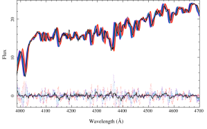
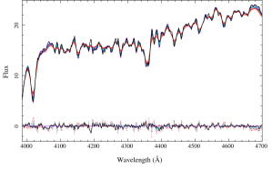
Figure 1: Left Panel: Detail of the central spectrum (5$\arcsec$ aperture, black solid-line) of NGC 2916 extracted from the V500 data cube of the CALIFA survey, together with the best fitted SSP template for the different scanned velocities (color-coded solid lines). The blueish solid lines correspond to SSP models blue-shifted with respect to the velocity, and the reddish solid lines correspond to red-shifted ones. Right Panel: Same spectrum shown in the left panel (black solid-line), together with the best fitted SSP template for the different scanned velocity dispersions (color-coded solid lines). The blueish solid lines correspond to SSP models with smaller velocity dispersion, while the reddish solid lines correspond to those with larger velocity dispersion. In both panels the residuals from the fits are plotted using the same color scheme, together with the residual of the best fitting model (grey solid-line). The two panels show two consecutive steps in the fitting procedure.

0.2 New Fitting philosophy of FIT3D

The main goal of any analysis pipeline dealing with IFS galaxy data is to disentangle the main components comprising the spatially resolved spectra. As in the case of long-slit or single-fiber spectroscopic data, the two main components are: (i) the light coming from the stellar population, that dominates the continuum and absorption spectrum, and (ii) the emission of the ionized gas, that is observable as a set of emission lines at certain characteristic wavelengths. The two components are affected by dust attenuation ($A_{V}$), produced by dust grains distributed across the galaxy (e.g. Tuffs et al., 2004). The disentanglement of these two main components is mandatory to properly study the properties of local and distant galaxies.

The rest-frame spectra of the two components are observed redshifted due the Doppler effect induced by the expansion of the universe and the residual velocity of the galaxy, and further blue- or red-shifted by the particular kinematics of the target cell, and component, within the galaxy. In addition, the spectra are broadened by a characteristic velocity dispersion, accounting for the unresolved kinematics that comprises the perturbations with respect to the average velocity pattern, and the non-homogeneous motions (such as non-circular motions). In rotational supported systems, like disks of spiral galaxies, the velocity dispersion is much lower than the asymptotic rotation velocity. On the other hand, in pressure supported systems, like bulge dominated early-type galaxies, the broadening from random orbits is much larger than pure rotation velocity. Obviously, this picture is an oversimplification, since many other components may affect the kinematics pattern, like bars, outflows, interactions, an so on (e.g. Barrera-Ballesteros et al., 2014). Irrespectively of the particular kinematic pattern, its effect has to be taken into account by any analysis pipeline.

Former versions of FIT3D address this problem by (i) modeling the continuum with a linear combination of synthetic stellar populations (SSP), and (ii) modeling the emission lines with a set of single Gaussian functions. Details of the procedures adopted to fit both components are given in the sections below. In the case of the stellar populations, their weights or eigen-values were derived without boundary constraints (Sánchez et al., 2006b, 2011). However, if any of the weights derived was found to be negative, the corresponding SSP was removed from the template list, and the fitting procedure was repeated until only positive weights were derived. Under this procedure, only a few number of SSPs remain in the final iteration, limiting the extracted information to the average properties of the underlying stellar population, like the luminosity or mass weighted ages and metallicities. This procedure was also very sensitive to the effects of noise, and did not allow to estimate the errors on any of the quantities derived. Despite these limitations, this approach provides a reliable subtraction of the underlying stellar population.

In the current version of FIT3D, we adopt a Monte-Carlo approach (MC), in which the previous procedure is iterated for a randomized version of the input spectrum taking into account the error vector. The individual weight vector is stored in each of the iterations. The final model of the stellar component is built using the mean weights derived along the MC sequence. In addition, this method provides realistic uncertainties of both the weights and the final model, based on the standard deviation with respect to the mean values. The details of how the MC is performed will be explained in the following sections.

Therefore, the analysis of the underlying stellar population, without considering the emission lines, comprises a non-linear and a linear problem. The non-linear problem includes the parameters that define the kinematic properties of the spectra and the dust attenuation, and the linear one involves the decomposition of the underlying stellar population in its components, either synthesized stellar populations (SSPs), or a library of stellar templates. The non-linear problem is addressed first and independently than the linear one.

The algorithms included in FIT3D were originally developed in perl, making an extensive use of the Perl Data Language (PDL ). We have developed a python version for which we have adopted most of the required algorithms included in PDL. The particularities of the python version will be described elsewhere (Ibarra et al., in prep.).

0.2.1 Non-Linear parameters of the stellar populations

Unlike other tools (e.g., pPXF Cappellari & Emsellem, 2004b), FIT3D was not developed to provide a detailed kinematic analysis of the line-of-sight velocity distribution. However, it estimates the main properties of the kinematic structure, i.e., the stellar velocity ($v_{sys}$) and velocity dispersion ($\sigma_{v}$). These parameters are derived under the assumption that all stellar populations move at the same velocity, with a velocity dispersion following a Gaussian function. This is clearly an approximation, since it is well known that the velocity distribution of stellar populations deviate strongly from this simple approach (e.g. Rix & White, 1992). However, most cases require a higher spectral resolution than the one presented here ($R<$2000) to make a clear distinction between this Gaussian approximation and more complex velocity distributions. The stellar kinematics is derived prior to the linear combination required to analyze the stellar population, based on an additional pseudo-random exploration within a pre-defined range of values. The pseudo-random exploration varies the parameter in question within a pre-defined range of values, but not following a fixed step. Instead it uses a random step, generated within a $\pm$50% of the original step (by default, 1/30th of the parameter range). This loop is repeated several times (three by default). We consider that this non-regular exploration of the parameter space provides a better sampling within the given range of values.

For the velocity dispersion we adopted two different implementations: (i) measuring it in units of wavelength, since for most of the spectra analyzed the dispersion is dominated by the instrumental one, and (ii) a different version that considers both a fixed instrumental dispersion along the spectral range in units of wavelength, and a physical velocity dispersion (in km/s). That second version requires a better knowledge of the instrumental dispersion and it is somewhat slower to run since it performs two different convolutions over the stellar templates.

In the first case, the stellar templates are convolved with a Gaussian function in wavelength space, and then shifted to the corresponding velocity. Although this is a crude approximation, for spectra dominated by instrumental resolution (e.g., PINGS and F-CALIFA data Rosales-Ortega et al., 2010; Mármol-Queraltó et al., 2011), there is no significant difference. In the second case, the stellar templates are first convolved in linear wavelength space with a fixed instrumental resolution (as in the first case), and then they are convolved in log($\lambda$) space with a Gaussian that accounts for both the velocity and the velocity dispersion.

The fitting sequence is as follows: First, the velocity dispersion is fixed to an input guess value, and the velocity is changed incrementally from a minimum to a maximum value, using a semi-random step around a certain fixed velocity step. For each velocity a best linear combination of SSPs that reproduces the continuum is derived, based on the reduced $\chi^{2}$. Then a range of velocity dispersions is explored, following a similar procedure, now fixing the velocity to the best result found in the previous step. The procedure is repeated twice, with the second iteration focused on the best parameters found in the first one, and reducing both the range and the size of the step to a 10% of the initial values. Figure 1 illustrates this process. It shows a detail of the central spectrum (5$\arcsec$ aperture), extracted from the V500 setup data cube of NGC 2916 from the CALIFA survey, together with the best SSP templates derived for each of the scanned velocities and velocity dispersions within the ranges considered.

Once the velocity and velocity dispersion are derived, then the range of dust attenuations that better reproduce the data is explored. Again, a range of values is explored between a minimum and a maximum dust attenuation, using a pseudo-random exploration with a variable step between consecutive values. Following the same procedure described before, the best linear combination of SSPs is derived for each particular value of the dust attenuation. Figure 2 illustrates this procedure. It shows the full wavelength range of the central spectrum (5$\arcsec$ aperture), extracted from the V500 setup data cube of NGC 2916 from the CALIFA survey, together with the best SSP templates derived for each of the scanned values of dust attenuation within a range between 0 and 1.6 mag.

Obviously, as described, this procedure would be computationally very intensive, and impractical in its current form. Thus we have implemented some modifications to speed-up the process: (i) The MC iterations on the linear combination of SSPs are not applied in the steps required to derive the velocity, velocity dispersion, and dust attenuation, thus, a single linear combination is derived for each step. The fitting is performed using a standard matrix inversion method to do a least squares minimization weighted by the errors, as implemented in the PDL routine linfit1d; (ii) a library with fewer number of single SSPs was adopted in these initial steps too (although it is not mandatory or restricted to do so); (iii) a restricted wavelength range could be considered for the derivation of the kinematic components, taking into account those regions with stronger stellar absorption features (e.g., 3700-4700 Å in the case of CALIFA and MaNGA data). This approach is new, since in general it was considered that using just the regions with stronger stellar absorptions would create a bias towards the velocity of the younger stars. Indeed, H-K Ca lines can be broadened due to the rotation of hot stars (e.g. Gerhard, 2003; Walcher et al., 2005). However, for the range of velocity dispersion expected in galaxies this seems not to have a strong effect, based on the tests that we have performed; (iv) a well defined range for the velocity and velocity dispersion is derived by analyzing the integrated spectrum and the central/peak spectrum for each galaxy. In this initial exploration a wider range of parameters is considered. Extensive tests have shown that these approaches do not affect the results within the expected uncertainties, as we will describe later.

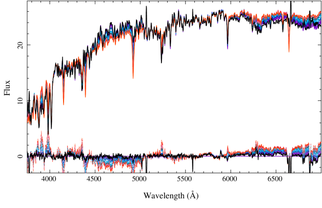
Figure 2: Central spectrum (5$\arcsec$ aperture, black solid line) of NGC 2916 extracted from the V500 data cube of the CALIFA survey, together with the best fitted SSP template for the different scanned dust attenuations ($A_{V}$) as color-coded solid lines ranging from $0$ to $1.6$ mag. The blueish solid lines correspond to SSP models with low dust attenuation, while the reddish solid lines correspond to those with larger attenuation. The residuals from the fits are plotted using the same color scheme, together with the residual of the best fitting model (grey solid line).

In all the three pseudo-random explorations, for each parameter we consider an input guess, a range of values, and an input step for which the parameter space is explored. The input guess is used as a fixed tracer of one of the parameters when the other two are explored. Therefore, the accuracy and precision of the derivation is limited to the input parameters injected. In order to perform the pseudo-random exploration, instead of using a constant step between the minimum and maximum, the step is variable within an 80% range of the input step. This ensures that the exploration is not uniform, and, due to the double iteration, it allows a better estimation of the parameter. For each iteration the best reduced $\chi^{2}$ derived from the linear analysis of the underlying stellar population is stored. Then, the minimum $\chi^{2}$ together with the two adjacent values are used to derive the parameter value using a parabolic minimum derivation (Sánchez, 2006a), together with a rough estimation of the error in the parameter as the range in which the reduced $\chi^{2}$ changes up to $\chi^{2}+1$.

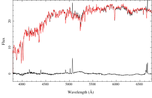
Figure 3: Left Panel: Detail of the central spectrum (5$\arcsec$ aperture, black solid line) of NGC 2916 extracted from the V500 data cube of the CALIFA survey, together with the different MC-realizations of this spectrum created along the fitting procedure (color-coded points). The real noise has been increased by a factor 5 to visualize the different realizations more clearly. The residuals from the best model fitted in each MC-realization are included using the same color code as the model, together with the average of the different residuals (solid black line). Right Panel: Same spectrum shown in the left panel (black solid line) together with the best fitted SSP template derived using the MC linear regression technique (red solid line). The residual from the best fitting model is shown as a solid black line.

0.2.2 Linear parameters of the stellar populations

Once the non-linear parameters are derived, they are fixed in the derivation of the properties of the underlying stellar population, reducing the problem to the solution of a linear combination of templates (SSPs).

The implementation of the multi stellar-population fitting technique used in this article was already described in Sánchez et al. (2006b, 2011). The basic steps of the fitting algorithm, spectrum by spectrum, are the following:

1. Read the input and noise spectra and determine the areas to be masked. Lets define $O_{i}$ as the observed flux at a certain wavelength $\lambda_{i}$, $\sigma_{i}$ as the noise level at the same wavelength, and $N$ the number of elements of the masked spectrum.

2. Create a Monte-Carlo realization of the data, adopting a Gaussian random distribution for the noise. Lets define $G_{i}$ as the MC-realization of the observed flux, defined as

   $$G_{i}^{k}=O_{i}+{R_{i}}\sigma_{i}$$

   where ${R_{i}}$ is a random value following a (-1,1) Gaussian distribution, and $k$ is the running index of the current MC realization.

3. Read the set of SSP template spectra, shift them to the velocity of the spectrum, convolve them with the velocity dispersion, and re-sample to the wavelength solution. Lets define $F_{ji}$ as the flux of the $i^{th}$ wavelength of the $j^{th}$ template (once shifted, convolved, and re-sampled), where $M_{0}$ is the total number of templates used.

4. Apply the derived dust attenuation to the templates. The attenuation law of Cardelli et al. (1989) was adopted, with a ratio of total to selective attenuation of $R_{V}$=3.1. Let us define $F_{ji}^{A_{V}}$ as the flux of the $i^{th}$ wavelength of the $j^{th}$ template, after applying the dust attenuation corresponding to a certain attenuation of $A_{V}$ magnitudes.

5. Perform a linear least-square fit of the input spectrum with the set of redshifted, convolved, and dust attenuated SSP templates. The fitting is performed using a standard matrix inversion method, weighted by the errors, as described before, based on the PDL routine linfit1d. Then it is adopted a modified $\chi^{2}$ as the merit function to be minimized, with the form:

   $$\chi^{2}=\frac{1}{N-M}\sum_{i=1}^{N}D^{2}_{i},$$

   where

   $$D_{i}=w_{i}\Big{(}G_{i}^{k}-\sum_{j=1}^{M}a_{j}F_{ji}^{A_{V}}\Big{)},$$

   In the above expression, $w_{i}$ is the weight of the $i^{th}$ pixel, defined as

   $$w_{i}=\frac{1}{\sigma_{i}^{2}},$$

   $a_{j}$ is the coefficient of the $j^{th}$ template in the final modeled spectrum, and $M$ is the number of templates considered in the fitting procedure. The actual number of templates included in the SSP-library depends on the science goals and the quality of the explored data. In our case for a typical $N\sim$2000, the number of templates if of the order of $M\sim$100. There is no general recommendation of how large should be $M$ to derive optimal results. It is therefore required to perform simulations to test it (e.g. Cid Fernandes et al., 2014). However, our experience indicates that it should not be larger than 2-3 types the typical signal-to-noise of the spectra, as a practical rule.

6. Determine for which templates within the library a negative coefficient is derived in the linear combination (i.e. $a_{j}<0$). These templates will be excluded from the next iteration of the fitting procedure, that will be resumed in step (5). At each iteration, $M$ is decreased by the amount of templates excluded. This loop ends once all the coefficients are positive. It is important to note here that excluding those templates within the library that produce negative values for the coefficients do not produce in general an increase of the reduced $\chi^{2}$ of the fitting. Therefore, to remove them do not decreases the goodness of the fitting in a systematic way. This procedure is adopted both in the linear and non-linear exploration of the parameters.

7. The modeled spectrum flux at $\lambda_{i}$ for the $k$th MC realization is given by

   $$S_{i}^{k}=\sum_{j=1}^{M}a_{j}^{k}F_{ji}^{A_{V}},$$

   where now $M$ considers only the templates with positive coefficients $a_{j}^{k}$.

8. The procedure is iterated for a fixed number of MC realizations ($K$) from step (ii). The final modeled spectrum, with its corresponding uncertainties at each $\lambda_{i}$, is given by the mean and standard deviation of the individual models for each realization of the MC iteration, at the given wavelength:

   $$S_{i}={\rm mean}(S_{i}^{1..K})$$

   $$\sigma_{S_{i}}={\rm stddev}(S_{i}^{1..K})$$

   The final reduced $\chi^{2}$ is then recomputed using this final average modeled spectrum. It is found that in general this $\chi^{2}$ is not significantly different that the individual ones for each of the MC realizations (the same is valid for the standard deviation, in a consistent way). This confirms the assumption that each individual fitting reproduce the analyzed spectrum equally well, and the final distribution is a more realistic description of the properties of the stellar population.

   The final coefficients of the SSP decomposition and the corresponding uncertainties are derived using a similar procedure:

   $$a_{j}={\rm mean}(a_{j}^{1..K})$$

   $$\sigma_{a_{j}}={\rm stddev}(a_{j}^{1..K})$$

   where $\sigma_{par}$ is the uncertainty associated with the corresponding parameter.

For practical reasons, the algorithm provides the fraction of the total flux contributed by each particular SSP within the library at a certain wavelength, and therefore a normalization wavelength is recommended, and the flux at that wavelength, to use the coefficients for further derivations in a more easy way. Let’s define $c_{j}$ as these relative flux fractions. Along this article we have adopted the normalization at 5500 Å, however, this is not mandatory..

In the derivation of the non-linear parameters a reduced version of this algorithm was adopted, excluding steps (2), (6), and (8). Thus, only a single linear least-square fit is applied, without cleaning the negative coefficients (that are normally absent when the template adopted is limited to a few stellar populations), and not iterating over a sequence of MC realizations.

This algorithm shares a basis with other procedures described in the literature (e.g., Cappellari & Emsellem, 2004b; Cid Fernandes et al., 2005; Ocvirk et al., 2006; Sarzi et al., 2006a; Walcher et al., 2006; Sánchez et al., 2007a; Koleva et al., 2009; MacArthur et al., 2009). If required, low frequencies in the spectrum can be fitted by adding a polynomial function to the fitted templates, or by multiplying them by that function. There are different origins for these low frequencies in the spectrum, mostly related with defects in the spectrophotometric calibration of the data or the stellar libraries adopted for the SSP templates (e.g. Cid Fernandes et al., 2013) They may also be related to the way that the synthetic populations are generated, like differences/errors in the adopted IMF or the stellar evolution models, being different for different stellar templates (e.g. Cid Fernandes et al., 2014). In the particular implementation shown along this article we have performed this correction only to subtract the stellar component to analyze the emission lines. However, for the full analysis of the stellar populations is not implemented. This is evident in the residuals shown in Fig. 3.

By construction, the fitting algorithm requires that certain regions in the spectrum are masked: (i) strong and variable night sky emission line residuals, (ii) regions affected by instrumental signatures, like defects in the CCD (e.g. dead columns) whose effect was not completely removed during the data reduction process, (iii) regions affected by telluric absorptions, not completely corrected during the flux calibration process, and (iv) regions containing strong emission lines from the ionized gas.

In the case of FIT3D a final iteration is implemented that makes this later masking not critical. It is possible to combine the analysis of the stellar population and emission lines fitting in a single iterative process in which, for each iteration, the best model of the emission lines is removed prior to the analysis of the stellar population. We will describe later this possibility.

0.2.3 Average properties of the stellar populations

Once the best model for the underlying stellar population is derived based on a linear combination of SSPs, it is possible to derive the average quantities that characterize this population. The most common parameters derived are:

• The luminosity-weighted log age ($Age_{L}$) and log metallicity ($Z_{L}$) of the underlying stellar population,

  $${\rm log}Age_{L}=\sum_{j=1}^{M}c_{j}{\rm log}Age_{j},$$

  and

  $${\rm log}Z_{L}=\sum_{j=1}^{M}c_{j}{\rm log}Z_{j},$$

  where $Age_{j}$ and $Z_{j}$ are the corresponding age and metallicity of the $j^{th}$ SSP template, and $c_{j}$ is the weight in light of each SSP. In this context we define $Z$ as the mass fraction of metals, i.e., elements heavier than Hydrogen and Helium..

  Hereafter, for the sake of simplicity, we will refer to the previous values as the ’luminosity-weighted age’ (instead of the more cumbersome luminosity-weighted logarithmic age). The reader should take into account that a different definition would be:

  $$Age_{L}=\sum_{j=1}^{M}c_{j}Age_{j},$$

  and

  $$Z_{L}=\sum_{j=1}^{M}c_{j}Z_{j},$$

  being the case that the logarithm of the later ones do not correspond to the former ones. Indeed the former ones are the geometrical average, weighted by the fraction of light corresponding to each single stellar population, while the later ones correspond to the arithmetic average. Since the time sampling of the stellar templates is logarithmic, we consider the former one a better representation of the average ages and metallicities in galaxies, although it is possible to derive any of them using the FIT3D output.

• The mass-weighted log age ($Age_{M}$) and log metallicity ($Z_{M}$) of the underlying stellar population,

  $${\rm log}Age_{M}=\sum_{j=1}^{M}c_{j}{\rm ML}_{j}{\rm log}Age_{j},$$

  and

  $${\rm log}Z=\sum_{j=1}^{M}c_{j}{\rm ML}_{j}{\rm log}Z_{j},$$

  where $Age_{j}$ and $Z_{j}$ are the same parameters described before, and ${\rm ML}_{j}$ is the mass-to-light ratio of the $j^{th}$ SSP template (i.e., $\frac{M}{L}$).

  Hereafter we will refer to them as the mass-weighted age and metallicity. Similar caveats should be applied to this definition as the one expressed regarding the luminosity-weighted ones.

• The average Mass-to-Light ratio,

  $$<{\rm ML}>=\sum_{j=1}^{M}c_{j}{\rm ML}_{j}$$

  that in general is not the same as the Mass-to-light ratio of the integrated spectra, that would be given by:

  $${\rm ML}=\frac{\sum_{j=1}^{M}M_{j}}{\sum_{j=1}^{M}L_{j}}$$

  where

  $$M_{j}=c_{j}{\rm ML}_{j}L$$

  and $L$ is the total luminosity of the spectrum.

• We define the star formation history (SFH) as the evolution of the star-formation rate along the time. To derive it, we define the mass of stars of a given age:

  $$M_{age}=\sum_{j=1}^{M}{\rm M}_{j}\leavevmode\nobreak\ \leavevmode\nobreak\ {\rm if}\leavevmode\nobreak\ \leavevmode\nobreak\ age_{j}=age$$

  .

  Now, we estimate the cumulative amount of mass up to a time $\tau_{age}$ where $\tau_{age}=\tau_{Universe}-age$ and $\tau_{Universe}$ is the age of the Universe at redshift zero. For doing so, we integrate the amount of stellar mass since the beginning of the cosmological time to that time ($\tau_{age}$):

  $$M_{age,c}=\sum_{j=1}^{M}{\rm M}_{j}\leavevmode\nobreak\ \leavevmode\nobreak\ {\rm if}\leavevmode\nobreak\ \leavevmode\nobreak\ age_{j}>age.$$

  From these cumulative masses it is possible to derive the star-formation rate (SFR) at any particular time,

  $$SFR_{\tau_{age}}=\frac{\Delta M_{age}}{\Delta age},$$

  the distribution of these SFR${}_{\tau_{age}}$ conforms the SFH as defined before.

  At any time the mass remaining in stars is derived by:

  $$M_{age,cor}=\sum_{j=1}^{M}f_{cor,j}{\rm M}_{j}\leavevmode\nobreak\ \leavevmode\nobreak\ {\rm if}\leavevmode\nobreak\ \leavevmode\nobreak\ age_{j}>age,$$

  where $f_{cor,j}$ is the correction factor that takes into account the mass-loss and mass lock into remnants, for each stellar population at the given age and metallicity (e.g. Courteau et al., 2014).

  For each spectrum, both the SFH and the SFR are not single parameters, but arrays of length the number of ages included in the SSP template library.

The luminosity-weighted ages and metallicities should be considered as the first momentum of the distribution of weights, or, in other words, the first momentum of the star formation and chemical enrichment histories (in logarithm scale as defined here). They differ considerably from the effective ages and metallicities, since they do not match in general with the corresponding values if the population was composed by a single SSP (Serra & Trager, 2007).

The luminosity-weighted ages and metallicities highlight the contribution of the young stellar populations (with a strong color effect), that are much more luminous for a certain mass than their older relatives. However, the mass-weighted ages and metallicities are less sensitive to the young stellar populations, and therefore trace better the bulk of the star formation history, rather than the more recent star-forming events.

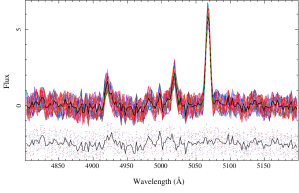
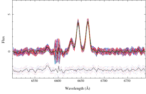
Figure 4: Left Panel: Detail of central spectrum (5$\arcsec$ aperture, black solid line) of NGC 2916 extracted from the V500 datacube of the CALIFA survey around the wavelength range of H$\beta$ and [O iii]$\lambda$4959,5007, together with the different MC-realizations of this spectrum created along the fitting procedure (color-coded points). The best fitting model to the emission lines is shown as green dashed line. The residuals from the different realizations are shown following the same color scheme (offset by -2.5 flux units for the sake of clarity), together with the residual of the best fitting model. Right Panel: Same spectrum shown in the left panel, but now around the wavelength range of H$\alpha$ and [N ii]$\lambda$6548,6583 (black solid line), together with the different MC-realizations of this spectrum created along the fitting procedure (color-coded points). The best fitting model to the emission lines is shown as a green dashed line. In both panels the level of noise has been increased by a factor 5 to visualize the different realizations more clearly.

0.2.4 Characterization of the emission lines

One of the goals of this fitting procedure is to provide an accurate characterization of the underlying stellar population, to subtract this contribution from the original spectrum, deriving an emission line only spectrum. This gas emission spectrum is derived by

$$C_{i}=O_{i}-S_{i}.$$

To measure the intensity of each emission line detected, each emission line in the clean spectrum ($C_{i}$) is fitted with a single Gaussian function, plus a low order polynomial. Following the new philosophy described below, the emission lines are fitted splitting the non-linear and the linear components. As in the case of the stellar population, the Gaussian function comprises two non-linear parameters, the velocity and velocity dispersion, and a linear one, the intensity. On the other hand, the polynomial function included to fit the continuum only comprises a combination of linear components. The procedure is very similar to the one outlined before. First, we perform an pseudo-random exploration of the non-linear parameters, within a range of values, starting with the velocity, and then the velocity dispersion. An initial guess of the velocity dispersion is used as a fix parameter in the exploration of the velocity, and later the velocity derived is fixed in the exploration of the velocity dispersion. In each step of the pseudo-random exploration a least-square linear regression is performed to derive the linear parameters (i.e., the intensity of each emission line and the coefficients of the polynomial function) by using the same standard matrix inversion method, weighted by the errors, described before, based on the PDL routine linfit1d. The reduced $\chi^{2}$ is stored in each iteration as a proxy of the the goodness of the fitting.. The final best combination of non-linear and linear parameters is derived on the basis of the minimization of the reduced $\chi^{2}$.

We estimate the errors of the optimized parameters by performing a MC simulation, where the original emission line only spectrum is perturbed by a noise spectrum that includes both the original estimated error and the uncertainties in the best fitted SSP model. Therefore, the intensity fitted at each wavelength $\lambda_{i}$ in each MC realization is

$$C_{i}^{k}=C_{i}+{R_{i}}\sigma_{{\rm modified},i}$$

where $i$ is the spectral pixel, ${R_{i}}$ is a random value following a (-1,1) Gaussian distribution, $k$ is the running index of the current MC realization, and

$$\sigma_{{\rm modified},i}=\sqrt{\sigma_{i}^{2}+\sigma_{S_{i}}^{2}}$$

where $\sigma_{i}$ is the original error (the one used in the analysis of the SSP), and $\sigma_{S_{i}}$ is the standard deviation around the best SSP model, $S_{i}$ (i.e., the uncertainty in this model) , as defined in point 8 of Sec. 0.2.2. Using this approach, we propagate the uncertainties of the subtraction of the underlying stellar population to the parameters derived for the emission lines.

Instead of fitting all the wavelength range at once, for each spectrum we extract shorter wavelength ranges that sample one or a few emission lines. This allows us to fit the residual continuum with the most simple polynomial function (in general, of 1st or 2nd order), and simplify the fitting procedure. When more than one emission line is fitted simultaneously, their velocities and dispersions may be coupled. Thus, they are forced to be equal in order to decrease the number of free parameters and increase the accuracy of the de-blending process (if required). This is particularly useful when the velocity dispersion is dominated by the spectral resolution, and for the recovery of the intensity of weak emission lines, with poorly defined kinematic properties. Figure 4 illustrates this procedure. It shows two spectral ranges centered in H$\beta$ and H$\alpha$, of the central spectrum of NGC 2916 shown in Fig. 1-3, once subtracted the best fitted SSP model shown in Fig. 3, together with the best fitted Gaussians to H$\beta$ and [O iii]$\lambda$4959,5007, and to H$\alpha$ and [N ii]$\lambda$6548,6583, respectively. The different MC realizations adopted during the fitting procedure are shown to illustrate how the procedure evaluates the parameters and errors at the same time.

A modeled emission line spectrum is created, based on the results of the last fit, using only the combination of Gaussian functions. This spectrum is given by

$$E_{i}=\sum_{k=1}^{L}B_{k}*{\rm Gauss}_{ik}(\lambda_{k},\sigma_{k}),$$

where $L$ is the number of emission lines in the model, $B_{k}$ is the integrated flux of the $k^{th}$ emission line, and ${\rm Gauss}_{ik}$ is the corresponding normalized ($\lambda_{k}$,$\sigma_{k}$) Gaussian evaluated at the $i^{th}$ pixel.

Finally, this modeled emission line spectrum is subtracted from the original spectrum ($G_{i}$), deriving an emission line free spectrum given by

$$GF_{i}=G_{i}-E_{i}.$$

This spectrum may be used to model again the stellar population, by applying the procedure described before, but without masking the emission line spectral regions, as outlined in Section 0.2.2. Actually, our experience is that adopting a simple SSP template library for the initial iteration, and a more detailed one for the second iteration produces very reliable results for both the emission lines and the stellar populations. In general, a third iteration does not produce any significant change in the properties derived, although the algorithm implemented allows the user to select the desired number of iterations. It is important to remark that the final reduced $\chi^{2}$ adopted includes both models and the propagation of the uncertainties.

The full data-flow described in the previous sections is summarized in Figure 5. In there, different steps of the fitting sequence are described, illustrating the products derived in each of them and the interdependence between those steps. The algorithm implemented in FIT3D allows the user to fit the stellar population without fitting any emission line, and at the same time it includes routines to fit the emission lines irrespectively of the underlying stellar population, in case that this is required.

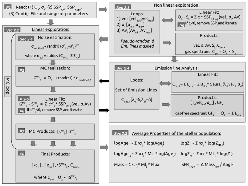
Figure 5: Chart-flow summarizing the fitting sequence of FIT3D as described in the text. The flow indicate the main blocks of the fitting process, indicating which operations are performed and the main data-products derived. The MC-loop is indicated with a bracket, and the final iteration over the emission-line fitting is indicating with black arrows. In each box a label indicate either the section in the text where the procedure is described or the point in Sec. 2.2 in which is explained.

0.3 Accuracy of the parameters derived

The procedure outlined above to fit the stellar population and the emission lines implements a somewhat new concept. It does not rely on minimization algorithms used frequently to fit non-linear functions, like the LM algorithm implemented in other tools (e.g., Gandalf, the previous version of FIT3D), but on a sequential combination of pseudo-random exploration of the range of non-linear parameters, and a least-square inversion of the linear ones. The MC realizations and pseudo-random explorations share some ideas with other tools that explore the properties of the stellar populations, like Starlight Cid Fernandes et al. (2005), however, their minimization scheme is based on a sequence of Markov chains, and not on a sequence of linear regressions.

Therefore, we need to demonstrate that the new procedure derives reliable results. To do so, we perform a set of simulations in order to determine that (i) the adopted procedure creates accurate models of the data, (ii) the main parameters of the stellar populations and emission lines correspond at least to the expected ones with respect to some well controlled inputs, and (iii) the procedure provides a reliable estimation of the uncertainties of the parameters derived.

0.3.1 SSP template library

As already noted by different authors (e.g. MacArthur et al., 2004; Cid Fernandes et al., 2014), this kind of analysis is always limited by the template library adopted, that comprises a discrete sampling of the SSP ages and metallicities. It is desirable that the stellar library be as complete as possible, and non-redundant. However, this would require an exact match between the models and the data, which is not possible to achieve in general, in particular if the stellar population comprises more than one SSP.

The results should be as independent as possible of the currently adopted SSP template library. Therefore, we have tested the fitting routines using different ones, following Cid Fernandes et al. (2014):

• gsd156 template library: described in detail by Cid Fernandes et al. (2013), it comprises 156 templates that cover 39 stellar ages (1 Myr to 13 Gyr), and 4 metallicities ($Z/Z_{\odot}=$ 0.2, 0.4, 1, and 1.5). These templates were extracted from a combination of the synthetic stellar spectra from the GRANADA library (Martins et al., 2005) and the SSP library provided by the MILES project (Sánchez-Blázquez et al., 2006; Vazdekis et al., 2010; Falcón-Barroso et al., 2011). This library has been extensively used within the CALIFA collaboration in different studies (e.g. Pérez et al., 2013; Cid Fernandes et al., 2013; González Delgado et al., 2014). Therefore, it is very interesting to know how accurate are our results using this particular library. Its spectral resolution has been fixed to the spectral resolution of the CALIFA V500 setup data (FWHM$\sim$6 Å).

• miles72 template library: It comprises 72 templates that cover 12 stellar ages (Myr to 12.6 Gyr), and 6 metallicities ($Z/Z_{\odot}=$ 0.015, 0.045, 0.2, 0.4, 1, and 1.5). These templates were extracted from the SSP library provided by the MILES project (Sánchez-Blázquez et al., 2006; Vazdekis et al., 2010; Falcón-Barroso et al., 2011). They do not cover as younger stellar populations as the previous ones, but they cover a wider range of metallicities. This template has a higher spectral resolution than the previous one, with FWHM$\sim$2.5 Å (Falcón-Barroso et al., 2011).

• bc138 template library: It comprises 138 templates that cover 23 stellar ages (1 Myr to 13 Gyr), and 6 metallicities ($Z/Z_{\odot}=$ 0.005, 0.02, 0.2, 0.4, 1, and 2.5). The SSP models were created using the GISSEL code (Bruzual & Charlot, 2003), assuming a Chabrier IMF (Chabrier, 2003). They cover a similar range of metallicities than the previous one, but with a wider range of ages. However, they do not benefit from the spectrophotometric accuracy of the MILES stellar templates (Sánchez-Blázquez et al., 2006). Its spectral resolution is slightly higher than the gsd156 one, with FWHM$\sim$5.5 Å.

• mar136 template library: It comprises 136 templates that cover 34 stellar ages (0.1 Myr to 15 Gyr), and 4 metallicities ($Z/Z_{\odot}=$ 0.05, 0.4, 1, and 2.23). The SSP models were created using the code by Maraston (2005), assuming a Salpeter IMF (Salpeter, 1955). They cover a slightly smaller range of metallicities than the previous one, but with a similar range of ages. It is the template with the lowest spectral resolution, FWHM$\sim$40 Å. This template was included to test the ability to recover the stellar population parameters when the spectral resolution is not very accurate.

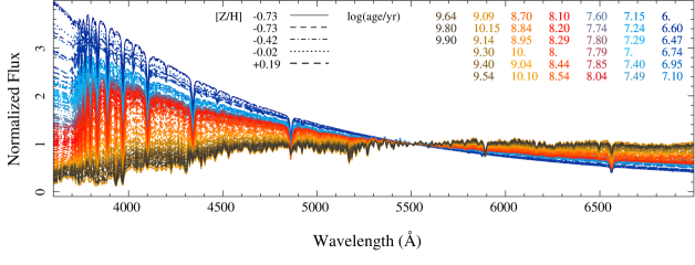
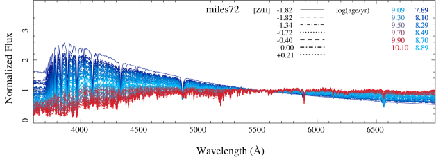
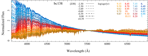
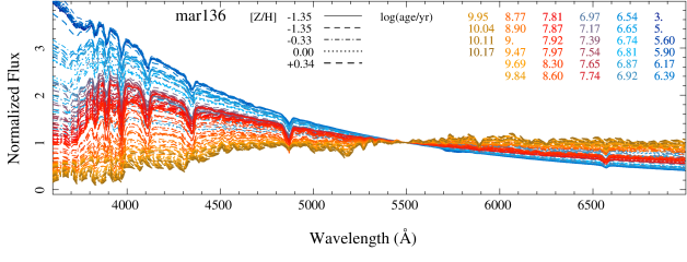
Figure 6: Stellar population templates included in the gsd156 (first panel), miles72 (second panel), bc138 (third panel) and mar136 (fourth panel) libraries. Each spectra within each library is represented with a different color, with the blueish colors representing the younger stellar populations, increasing the age towards more reddish/orange/grey colors.

The ranges of shapes covered by the different SSPs and how they compare with each other is shown in Figure 6. For each SSP library we present the individual spectra within the wavelength range corresponding to the optical range between 3700-7000Å, normalized at 5500Å. We note that the sampling of all of these libraries is different in the age distribution and in the metallicity one. This is intrinsic to the templates, and imposes a bias in the sampling of the properties, that is not intrinsic to FIT3D. In addition, none of these libraries includes the nebular continuum, to our knowledge, which may produce a significant effect for very young stellar populations.

There are several caveats when applying model SSPs to the integrated light of an entire galaxy, or a portion of it, which have been clearly identified by previous authors (e.g. MacArthur et al., 2004; Cid Fernandes et al., 2014). The most important one is to assume that the parameter space covered by the empirical library represents well that of the real data. However, in general, libraries are based on stars in the solar neighborhood (e.g. Sánchez-Blázquez et al., 2006) or synthetic models (e.g. González Delgado et al., 2005; Maraston, 2005), and therefore it is not granted that they represent well the stellar populations in other galaxies (or even in other regions of our Galaxy). Most of these problems are not particularly important in the context of our tests, since our primary goal is to determine the accuracy and precision of the parameters recovered for a set of simulated data; however, they do affect the interpretation of the results.

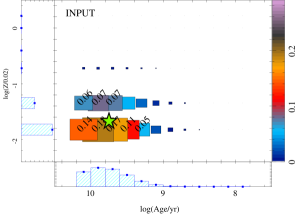
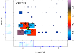
Figure 7: Left panel: Distribution of input coefficients along the age-metallicity grid for a single simulated spectrum corresponding to the first set of simulations, i.e., those resembling a single burst of star-formation, with a broad extension in time. This particular example corresponds to a simulation based on the miles72 template library. For each age-metallicity pair it is shown the weight as a solid square, with the size and color being proportional to the weight of the corresponding SSP_age,met. For those SSPs with stronger contribution (above a 5%), the actual fraction is indicated on top of each square. The horizontal and vertical histograms represent the co-added coefficients for a particular age and metallicity respectively. The green solid-star indicates the location of the luminosity weighted age and metallicity corresponding to the distribution of stellar populations: log(age/yr)=9.76, log(Z/0.02)=-1.68. Right panel: Similar distribution corresponding to the coefficients recovered for the given input simulation of a spectrum with a signal-to-noise ratio of $\sim$100, once the fitting procedure is applied. The green solid-star indicates the location of the luminosity weighted age and metallicity corresponding to the recovered distribution of stellar populations: log(age/yr)=9.78, log(Z/0.02)=-1.56.

In addition, it is important to note that the treatment of the dust attenuation may affect the resulting parameters (i.e. the luminosity-weighted age and metallicity of the stellar population). In this particular implementation of the analysis we adopted the Cardelli et al. (1989) attenuation law, which may not be the optimal solution to study the dust attenuation in star forming galaxies (e.g. Calzetti, 2001). Other authors, MacArthur et al. (2009) adopted a completely different attenuation law, based on the two-component dust model of Charlot & Fall (2000), which is particularly developed to model the dust attenuation in star forming galaxies. The differences between the existing extinction laws in the optical wavelength range (3600-10000 Å) are too small to affect significantly the results. Indeed, no major differences are found when adopting the Cardelli et al. (1989), Calzetti (2001), or even a simple $\lambda^{-1.3}$ extinction law. FIT3D adopted a fixed specific dust attenuation of R${}_{V}=$3.1 (i.e., Milky-Way like), and the only fitted parameter is the dust attenuation at the $V$-band ($A_{V}$), in magnitudes.

Table 1: Results of the simulations: Single Burst.

Results using the gsd156 SSP template
S/N	$\Delta$Age/Age	$\Delta$Z/Z	$\Delta$AV1	$\Delta$vsys1	$\Delta$$\sigma_{v}$1	$r_{cor}$2
64.4	0.17 $\pm$0.11	0.07  $\pm$0.10	-0.06 $\pm$0.17	0.6 $\pm$ 40.9	-34.4 $\pm$39.3	0.38
32.9	0.16 $\pm$0.21	0.05  $\pm$0.19	-0.08 $\pm$0.18	2.5 $\pm$ 49.5	-41.2 $\pm$45.4	0.38
6.8	0.12 $\pm$0.27	0.00  $\pm$0.21	-0.07 $\pm$0.26	-22.6 $\pm$111.9	-87.1 $\pm$69.2	0.31
3.4	0.09 $\pm$0.31	0.00  $\pm$0.24	0.05 $\pm$0.32	-38.1 $\pm$208.40	-104.4 $\pm$74.1	0.24
Results using the miles72 SSP template
S/N	$\Delta$Age/Age	$\Delta$Z/Z	$\Delta$AV	$\Delta$vsys1	$\Delta$$\sigma_{v}$1	$r_{cor}$2
70.6	0.07 $\pm$0.15	-0.05  $\pm$0.31	-0.02 $\pm$0.17	-2.5 $\pm$ 37.7	-14.2 $\pm$23.8	0.58
35.7	0.07 $\pm$0.15	-0.01  $\pm$0.35	-0.02 $\pm$0.18	-6.2 $\pm$ 43.3	-19.5 $\pm$31.1	0.57
7.2	0.09 $\pm$0.25	0.04  $\pm$0.48	-0.07 $\pm$0.28	-42.0 $\pm$150.0	-72.8 $\pm$66.7	0.52
3.5	0.03 $\pm$0.32	0.06  $\pm$0.50	0.00 $\pm$0.35	-101.6 $\pm$222.2	-92.4 $\pm$74.0	0.39
Results using the bc138 SSP template
S/N	$\Delta$Age/Age	$\Delta$Z/Z	$\Delta$AV	$\Delta$vsys1	$\Delta$$\sigma_{v}$1	$r_{cor}$2
65.4	0.09 $\pm$0.50	0.17  $\pm$0.64	-0.10 $\pm$0.35	6.7 $\pm$ 37.1	-55.7 $\pm$45.3	0.44
34.3	0.13 $\pm$0.48	0.16  $\pm$0.66	-0.12 $\pm$0.35	0.1 $\pm$ 79.0	-63.8 $\pm$48.8	0.44
6.8	0.11 $\pm$0.45	0.10  $\pm$0.68	-0.10 $\pm$0.68	-0.4 $\pm$105.2	-94.8 $\pm$64.7	0.45
3.4	0.04 $\pm$0.44	0.15  $\pm$0.75	-0.03 $\pm$0.34	-15.1 $\pm$113.3	-108.7 $\pm$65.2	0.47
Results using the mar136 SSP template
S/N	$\Delta$Age/Age	$\Delta$Z/Z	$\Delta$AV	$\Delta$vsys1	$\Delta$$\sigma_{v}$1	$r_{cor}$2
66.0	0.04 $\pm$0.30	0.25  $\pm$0.41	-0.15 $\pm$0.28	16.9 $\pm$ 59.0	-77.7 $\pm$72.8	0.53
35.6	-0.05 $\pm$0.39	0.32  $\pm$0.43	-0.09 $\pm$0.28	-2.0 $\pm$ 75.2	-91-3 $\pm$70.3	0.54
7.8	0.10 $\pm$0.38	0.07  $\pm$0.49	-0.15 $\pm$0.31	-88.1 $\pm$243.5	-110.7 $\pm$72.8	0.51
3.5	0.16 $\pm$0.43	-0.01  $\pm$0.53	-0.22 $\pm$0.36	-134.1 $\pm$260.4	-117.8 $\pm$76.0	0.57
Results using the gsd156 SSP template, fitted with the gsd32 template
S/N	$\Delta$Age/Age	$\Delta$Z/Z	$\Delta$AV1	$\Delta$vsys1	$\Delta$$\sigma_{v}$1	$r_{cor}$2
63.6	0.14 $\pm$0.20	0.08  $\pm$0.17	-0.08 $\pm$0.19	3.9 $\pm$ 25.8	-35.0 $\pm$38.0	0.33
32.2	0.13 $\pm$0.21	0.07  $\pm$0.20	-0.08 $\pm$0.20	1.6 $\pm$ 44.6	-42.3 $\pm$43.2	0.29
6.9	0.10 $\pm$0.25	-0.01  $\pm$0.22	-0.07 $\pm$0.21	-24.1 $\pm$133.1	-83.5 $\pm$67.3	0.19
3.4	0.07 $\pm$0.34	-0.01  $\pm$0.25	-0.04 $\pm$0.34	-49.1 $\pm$204.6	-104.9 $\pm$74.4	0.17

Each row shows the results of 1000 simulations, corresponding to a different S/N level, for each particular stellar template. Therefore, the errors in the derived offsets are a factor $\sqrt{1000}$ smaller than the values listed in the table.. ⁽¹⁾ The dust attenuation $A_{V}$ is in magnitudes, while the units of the velocity and velocity dispersion are km/s. ⁽²⁾ Correlation coefficient between $\Delta$Age/Age and $\Delta$Z/0.02.

0.3.2 Accuracy of the properties of the stellar population

As mentioned before, the main parameters derived from the analysis of the stellar component are (i) the coefficients of the SSP templates in which the stellar continuum is decoupled, (ii) the luminosity- and mass-weighted ages and metallicities, and dust attenuation, (iii) the stellar mass-to-light and mass comprised in the spectrum, and (iv) the star formation history. In order to assess the accuracy and precision of these parameters we have performed a set of simulations. The simulations should be performed trying to match as closely as possible some real data, especially the noise pattern. Since the primary goal of the currently developed package is the analysis of IFU data extracted from the CALIFA data, we will limit our tests to the wavelength range and spectral resolution of the CALIFA-V500 setup (Sánchez et al., 2012a): a wavelength range between 3700-7500 Å, and an instrumental resolution of $\sigma_{inst}=$2.6 Å. However, the simulations can be easily adapted to any other spectroscopic configuration.

The noise pattern is composed, in general, of both white noise (corresponding to the photon-noise of the source and the background, and electronic noise from the detector), and non-white noise (corresponding to defects/inaccuracies in the sky-subtraction, uncorrected defects in the CCD, errors in the spectrophotometric calibration, etc). These noise patterns are different spectrum-to-spectrum, and wavelength-to-wavelength, and are clearly difficult to simulate on a simple analytical basis. However, for a general test like the one performed here, we will limited our simulations to the use of white noise. In forthcoming articles we will explore the accuracy and precision of the parameters recovered using a more ad hoc set of simulations, following Cid Fernandes et al. (2014).

We perform two different sets of simulations. In the first one, a SFH dominated by a single burst of star formation is assumed, and therefore the stellar populations are dominated by stars of a certain age. The burst follows a Gaussian shape, with a width 0.5 dex in age (i.e., the length of the burst is proportional to the age selected). Under this assumption the burst lasts for a longer time at earlier times, and it is much shorter at later times. For the metallicity, we considered a similar probability distribution. Therefore, the simulated stellar population is dominated by stars of a certain metallicity with a Gaussian distribution of-width of 0.5 dex at each metallicity. This does not attempt to model any real physical enrichment mechanism in particular. Each simulated stellar spectrum is created by randomly selecting (within the range of the values considered in the SSP template) a particular age and metallicity as the center of the 2D Gaussian distribution.

In general, this simulated SFH may not be realistic. In most SFHs analyzed within the CALIFA survey most of the stars are formed following an exponential law with more than 80% of the mass formed in the first few Gyr (Pérez et al., 2013). If we assumed this more realistic SFH we would not be able to test the ability of the fitting tool to decouple different stellar populations, and we would just test the very particular case that is more frequently observed in the Local Universe.

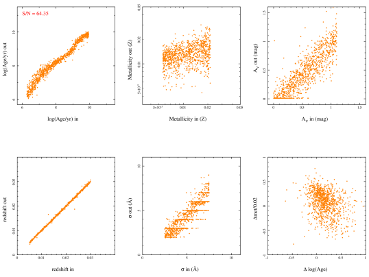
Figure 8: Results from the simulations. From left to right and from top to bottom, each panel shows the comparison between the input luminosity-weighted age, metallicity, dust attenuation, redshift, and velocity dispersion with the values recovered by our fitting technique. In addition, the degeneracy between different parameters is explored, showing a comparison of the differences between the input and output values for age and metallicity, age and velocity dispersion, metallicity and velocity dispersion, and age and dust attenuation. The results are presented for the gsd156 template and the simulations for a S/N$\sim$60.

In the second set of simulations we try to create a more realistic SFH, in which the contribution of a stellar population within the template is proportional to a power of its age in Gyr ($a_{j}\propto Age_{j}^{1/2}$). This is basically an exponential star formation rate along the evolution of the stellar population. The metallicity distribution follows a Gaussian probability function similar to the one described before. However, in this particular case the input metallicity is forced to follow a linear anti-correlation with age; i.e., older stellar populations are more metal poor than younger ones, following the recent results by González Delgado et al. (2014).

Results from the single burst simulation

For the first single burst SFH we create four different sets of simulations. In each one, 1000 simulated spectra were created with the same normalized flux at 5000 Å, corresponding to 100, 50, 10 and 5 10^-16 erg s^-1 cm^-2 Å^-1, respectively. The velocity was randomly selected within the redshift range of the CALIFA footprint ($0.005<z<0.03$), and the velocity dispersion was selected randomly from $\sigma=2.5-7.5$ Å ($\sigma_{v}\sim 100-400$ km/s). Then, the simulated spectrum was reddened by a dust attenuation randomly selected between $A_{V}=0-1.1$ mag. Finally, a purely poissonian noise was added, to a level of 1 10^-16 erg s^-1 cm^-2 Å^-1. As indicated before, this is not a totally realistic noise pattern. However, to perform a more detailed simulation it would require to adopt ad hoc noise patterns, attached to a particular data set (e.g. Sánchez et al., 2011).

The fitting procedure was then applied to the simulated spectra using the same steps adopted to analyze the observational data, deriving, for each one, the different data products described in Sec. 0.2.3. Figure 7 illustrates the result of this exercise for a particular spectrum with a signal-to-noise ratio of $\sim$100. It shows the input coefficients for a particular simulated spectrum created using the miles72 template library (for both the simulation and the analysis), in comparison with the output distribution. This kind of distribution comprises the star-formation history and metal enrichment pattern, that are projections of this distribution. It is clear that the luminosity weighted values derived from both distributions are very similar (log(age/yr)_in=9.76 vs. log(age/yr)_out=9.78 and [Z/H]_in=-1.68 vs. [Z/H]_out=-1.56 ), despite the fact that there are clear fluctuations between the input and recovered weighted/contributions of each particular stellar component. The largest discrepancy is for the lower metallicity bin and the log(age/yr)=9.50 component, that differs about a 10% each one. Furthermore, the distribution of coefficients in the age-metallicity grid is remarkable similar. Similar analyzes were performed by Ocvirk et al. (2006), Koleva et al. (2009), and Sánchez et al. (2011), although they cover a more reduced parameter space, and in general the kinematics and/or the dust attenuation were fixed in their simulations.

Table 1 lists, for each set of simulated spectra, their average signal-to-noise ratio and the difference between the input and the recovered values for the following parameters: luminosity-weighted age, metallicity, and dust attenuation, together with the velocity and velocity dispersion, with their corresponding standard deviation. Here we are measuring two different effects: (i) the systematic deviation from the input parameters, characterized by the average offsets, (i.e., the accuracy of the measurement) and (ii) the precision in the measurement of the parameter (with or without a systematic bias or offset), characterized by the standard deviation. This corresponds to the expected the precision of each individual realization. However, the error of the systematic deviation described before is $\sim$30 times smaller, taking into account that each row corresponds to 1000 independent simulations. Only in the case that the average offset is clearly larger than this error it is possible to claim that there is a systematic offset for all the simulated dataset. This is more evident for the spectra with high S/N , where the systematic effects dominate over the precision of the measurement. However, in most of the simulated dataset there is a clear and well defined bias with similar trend for each different template, despite of the estimated precision. Nevertheless, if the standard deviation is clearly larger than the derived offset, the expected bias for an individual realization is too small compared with the systematic bias/offset and therefore is sub-dominant. This is the case for most of the values in the table, and in particular for the spectra with lower S/N.

There are large differences between the accuracy and precision of the recovered parameters depending on the adopted stellar templates. For those templates with higher spectral resolution, miles72 and gsd156, the parameters are recovered with a better accuracy and precision for the spectra with higher signal-to-noise ratio. In those cases the standard deviation and the offsets between the input and output values are smaller, irrespectively of the possible systematic offsets. Those offsets are in general smaller than the standard deviations, and therefore they are sub-dominant for individual realizations, although in general they are statistically significant.

In summary, the simulations indicate that it is possible to recover the properties of the stellar populations for at least a S/N of $\sim$ 30-50 per pixel to derive accurate and precise results in this particular case. However, for those templates with coarser spectral resolution the parameters are recovered equally well/bad for a wide range of S/N. Figure 8 illustrates these results, showing for a particular set of simulations the comparison between the input and recovered parameters for each individual spectrum in the dataset. In some cases, like in the age-age comparison, there are clear structures that indicates a possible bias in the recovery of this parameter.

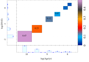
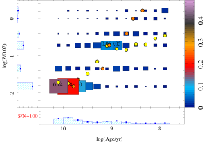
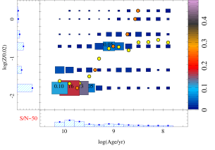
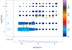
Figure 9: Top-Left panel: Input coefficients distribution along the age-metallicity grid for a simulated spectrum corresponding to the second set of simulations, i.e, those resembling a star formation history with a continuous declining star formation rate, using the miles72 template library. For each age-metallicity pair the weight is shown as a solid square, with size and color proportional to the weight of the corresponding SSP_age,met. For those SSPs with a stronger contribution, the actual fraction is indicated on top of each square. The horizontal and vertical histograms represent the co-added coefficients for a particular age and metallicity respectively. Top-Right panel: Similar distribution corresponding to the coefficients recovered for a spectrum with a signal-to-noise ratio of $\sim$100. The yellow filled circles show the average metallicity for a given age, while the orange filled circles show the average age for a given metallicity. Bottom-left panel: Similar distribution as shown in the previous panel but for a simulated spectrum with S/N$\sim$50. Bottom-right panel: Similar distribution as shown in the previous panel but for a simulated spectrum with S/N$\sim$10.

A comparison of the offset between the output and input values for different parameters is also explored to understand the possible degeneracies among them. It particular, we explore the possible bias introduced by the age-metallicity degeneracy: In general older stellar populations are redder, like metal rich ones, while younger and metal poor ones are bluer (Worthey, 1994). This introduces a degeneracy in the derivation of both parameters, as discussed by previous authors (e.g. Sánchez-Blázquez et al., 2011). The strength of this degeneracy is parametrized by the correlation coefficient, $r_{cor}$, between both parameters, listed in Table 1. The correlation shows a similar behavior for the different stellar templates when S/N>10. The offset in age and metallicity is in most cases of the order of $r_{cor}\sim$0.4-0.5.

The age-metallicity degeneracy shows the second strongest correlation. The weakest ones have not been included in the figure. They correspond to the possible degeneracy between the metallicity and both the dust attenuation and the velocity dispersion, that are of the order of $r_{cor}\sim 0.1$. Thus, there is no degeneracy between those parameters. The offset in age present a weak trend with the offset in velocity dispersion, with a typical $r_{cor}\sim$0.3. Finally, the strongest correlation is found between the offset of age and the offset of dust attenuation, for which the correlation is strong ($r_{cor}\sim$0.8) in all the cases explored. This degeneracy is a well known one that indicates how important it is to have a good determination of the dust attenuation to derive the ages. This degeneracy affects more to the younger than to the older stellar populations.

It is beyond the goal of this study to make a comparison between the properties of the different SSP libraries discussed here. We used different ones to illustrate that the procedure is able to recover the input parameters independently of a particular library. However, it is clear that there are differences. This is the case of the already quoted miles72 and gsd156 templates, when compared with the bc138 one. The accuracy of the derived parameters is very similar in the three cases (as estimated by the bias/offset). However, the precision is much worst for the later one. By far, the parameters are recovered with less precision when using the libraries bc138 and mar136. This may reflects subtle effects of how the space of parameters is coveraged, differences in the stellar templates adopted, or details in the code that generate the templates. For example, the miles72 template does not include SSPs younger than 60 Myr, while the gsd156 template does not include SSPs more metal poor than 0.2 $Z_{\odot}$, while the range of parameters covered by bc138 includes both of them. Finally, the bc138 template uses the STELIB stellar library (Le Borgne et al., 2003), which spectrophotometric calibration along the full wavelength range is worse than the one presented by the MILES one (Sánchez-Blázquez et al., 2006). We have repeated analysis based on the bc138 library restricting its age/metallicity coverage to that of the miles72 and gsd156. Only in the case of the metal-rich version of the library there is an improvement on the accuracy and precision of the recovered parameters. However it never reach the values found for the two later libraries. Therefore, although the coverage in the age/metallicity space has an effect on the results of the simulations, biasing towards those libraries with lower metallicity range, it cannot explain totally the reported differences.

Finally, the mar136 library has the lowest spectral resolution, that strongly affects the results. A detailed discussion of the expected differences when using different stellar templates can be found in (González Delgado et al., 2015). For the other libraries, the stellar age, dust attenuation, and stellar velocity properties are recovered well, although there is a wide range in the accuracy and precision of the properties derived, as summarized in Table 1. For the SSP libraries with the better spectral resolution, and for S/N$>$50, the precision is of the order of $\sim$0.1-0.2 dex, similar to the one reported by other fitting procedures (e.g., starlight, Cid Fernandes et al., 2014). The reported uncertainties are slightly larger than the ones estimated for other codes, like Steckmap (Ocvirk et al., 2006; Sánchez-Blázquez et al., 2011). Ocvirk et al. (2006) found a typical error $\Delta age=0.06-0.09$ dex and $\Delta met=0.10-0.14$ dex, for signal-to-noise ratios of 50 and 20 respectively, and a spectral resolution $R=1000$. However, in these latter simulations the effect of the precision of the velocity dispersion and the dust attenuation was not taken into account. Using a similar code, Sánchez-Blázquez et al. (2011) found that there is an intrinsic uncertainty in the derivation of the parameters associated with the velocity dispersion, a trend already reported by Koleva et al. (2009).

The velocity dispersion is recovered better for those stellar templates with higher spectral resolution (e.g., miles72), and worse for those with lower spectral resolution (e.g., mar136). Unexpectedly, the velocity does not present the same trend. There is an updated version of the Maraston (2005) SSP models with higher spectral resolution, based on different empirical and theoretical spectral libraries (Maraston & Strömbäck, 2011). They cover a similar range of ages as the templates outlined here, however, they do not cover the same range of metallicities for the younger stellar ages. In general, they produce similar results than the ones provided by the miles72 and gsd156 models. Therefore, the main differences described here are introduced by the coarse spectral resolution of the Maraston (2005) models. When the updated/higher-resolution version is used, we find no significant differences.

The age-metallicity degeneracy is weaker for the high signal-to-noise simulations for the gsd156 and mar136 libraries, slightly larger for bc138, and clearly stronger for miles72. However, in all cases the correlation is significant, with a probability of not being produced by a random distribution of the data larger than a 99.99%. In the case of the bc138 library the same reason outlined before for the larger error in the parameters recovered could explain this small increase in the degeneracy. In the case of miles72, the fact that this library does not include stellar populations younger than 63 Myr could produce that effect, since the algorithm tries to compensate the absence of these young stellar populations giving more weight to more metal poor ones. Finally, we notice that for some templates the strength of the degeneracy decreases with increasing noise, which indicates that for noisy spectra the random error dominates over this systematic bias (e.g., gsd156 and miles72). However, for other templates, the strength is enhanced by the noise (e.g. mar136), highlighting the effect of a coarse spectral resolution in the degeneracy between both parameters.

A possible source of error in the interpretation of these simulations is the fact that the same set of templates was used to create the simulated data and to model them. In principle, we assumed that the grid of templates is representative of the real stellar population of the spectra analyzed, but it is likely that this library is incomplete. This is not the case in our simulations, by construction. To study the effects of this possible incomplete representation of the observational spectra by the template library, we created a new set of simulated data using the gsd156 library, that was then fitted using a much reduced version of the template library, that we called gsd32. This template comprises a grid of 32 SSPs, corresponding to 8 ages covering the same range than gsd156, and with the same 4 metallicities. The results from this simulation are listed in Table 1. It shows that in the case of an incomplete sampling of the spectroscopic parameters by the model template, these parameters are still well reconstructed, albeit with a lower precision (as expected). We repeated the experiment with an even more reduce set of stellar libraries, with only 12 SSPs, with a similar result. It is important to note that in both cases the more extreme stellar populations from the original template were retained in the restricted one (i.e., the oldest/youngest and more metal rich/poor). Finally, we want to remark that although the average parameters that characterize the stellar populations are still recovered well, the details of the SFH and chemical enrichment are lost, obviously.

Results from the simulated SFH

The second set of simulations is created to follow a more realistic SFH. We create three different sets of simulations, each one comprising 1000 simulated spectra with the same normalized flux at 5000 Å, corresponding to 100, 50 and 10 10^-16 erg s^-1 cm^-2 Å^-1, respectively. The velocity, velocity dispersion, and dust attenuation were taken into account in a similar way as in the previous set of simulations described in Sec. 0.3.2. For this study we show only the results using the miles72 template library, although we have repeated all the analysis using the other libraries with similar results.

The fitting procedure was then applied to the simulated spectra using the same steps adopted to analyze the observational data, deriving, for each one, the different data products described in Sec. 0.2.3. Figure 9 illustrates the result of this exercise for three particular spectra, each one corresponding to a different S/N level. It shows the input coefficients for a particular simulated spectrum in comparison with the output distribution. It is clear that both the SFH, represented by the histogram in the bottom of each panel, is well reproduced for the different simulated spectra, although as expected, the input shape is more and more diluted as the S/N decreases. The metal enrichment pattern is well reproduced in any of the simulations, being more accurate for the older stellar populations than for the younger stellar populations. The distribution of metallicities at different ages and ages at different metallicities, represented in the figure as yellow and orange solid circles, are a relatively good representation of the input correlation between the metals at different ages; thus, they are good tracers of the metal enrichment pattern.

Table 2: Results of the simulations: simulated SFH.

S/N	$\Delta$Age/Age	$\Delta$Z/Z
118.0	-0.12 $\pm$0.02	0.01  $\pm$0.03
59.7	-0.14 $\pm$0.03	0.03  $\pm$0.04
11.9	-0.20 $\pm$0.10	0.08  $\pm$0.15

Table 2 lists, for each set of simulated spectra, their average signal-to-noise ratio and the difference between the input and the recovered values for two of the parameters derived: luminosity-weighted age and metallicity. The kinematics and dust attenuation values are not listed since they do not present significant differences with the previous simulations, due to the decoupling of the derivation of these properties and the derivation of the SFH, as described in Sec. 0.2. We note that the precision of the parameters recovered is better for this more realistic SFH than for the single-burst one, described in Sec. 0.3.2, even for low S/N spectra. In general, the two luminosity-weighted parameters are recovered with a precision better or of the order of 0.1 dex.

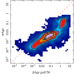
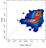
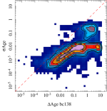
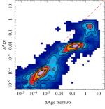
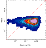
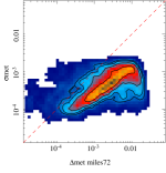
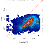
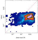
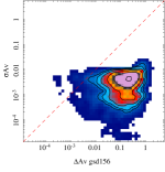
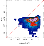
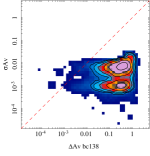
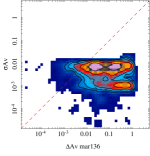
Figure 10: Distribution of the estimated errors for the different parameters derived for the stellar populations, luminosity-weighted age (top panels), metallicity (middle panels), and dust attenuation (bottom panels), along with the absolute difference between the output and input parameter for the first set of simulations described in Sec. 0.3.2. Each panel, from left to right, corresponds to a different stellar template library considered in the simulations. For each panel the contours correspond to the density of points, with the first contour encircling 95% of the points, and each consecutive contour encircling 15% less number of points.

Accuracy on the estimated errors

The two main goals of the current modification of FIT3D with respect to previous versions, regarding the analysis of the stellar populations are: (i) to provide with a reliable estimation of the star formation history and the average properties describing the stellar population, and (ii) to obtain a useful estimation of the uncertainties of the parameters derived. In previous sections we have illustrated how well are recovered the parameters that describe the underlying stellar population. In this section we explore how representative are the estimated errors of the real uncertainties in these parameters. For doing so we used the first set of simulations, described in Sec. 0.3.2, that cover a wider range of parameters, and we compare the errors estimated by the fitting procedure ($\sigma{\rm PAR}$) with the absolute difference between the recovered and the input parameters ($\Delta{\rm PAR}$), where ${\rm PAR}$ is the parameter considered: age, metallicity, or dust attenuation ($A_{V}$).

FIT3D estimates the error of each parameter based on the individual values derived along the MC-chain of realizations described in the previous sections. The best fitting model is derived for each MC realization, and therefore, the best set of parameters that describe the input spectrum. It is generally assumed that the standard deviation of the values derived for each parameter is a good representation of the real errors ($\sigma{\rm PAR}$). Indeed, this is the basic assumption of any MC or bootstrapping procedure aimed to estimate the errors in any analysis. However, this assumption holds if the different parameters are independent, and if the errors affect equally each of them. Therefore, there is no guarantee that $\sigma{\rm PAR}$ is indeed a good representation of the real uncertainty in the derivation of the parameter.

Figure 10 shows the distribution of $\sigma{\rm PAR}$ along $\Delta{\rm PAR}$, for the three parameters, and for each of the stellar template libraries described before. The patterns in the comparison between the estimated and real errors are very similar for the different stellar templates, with most of the differences due to the ranges covered in age and metallicity. First, it seems that the errors derived by the fitting procedure are a good trace of the real differences between the input and recovered values, for both the luminosity-weighted age and metallicity, with a global underestimation of the real errors by a factor $\sim$4, $\Delta{\rm Age}\sim 4\sigma{\rm Age}$, and $\Delta{\rm met}\sim 4\sigma{\rm met}$. For those libraries with a smaller range of age or metallicity the trend between both errors is less obvious, as expected since the dynamical range of parameters is less well covered.

For the dust attenuation, there is also a bias between the recovered and real error, but it is less obvious that the estimated error is a good estimation of the precision of how this parameter is recovered. Indeed, in general it seems that the dust attenuation is recovered with an average uncertainty of $\sim$0.1-0.3 dex, without a clear correspondence with $\sigma{\rm A_{\rm V}}$. However, we must recall that the error in the dust attenuation was not estimated on the basis of a MC-scheme, and it corresponds to the value estimated from the $\chi^{2}$ curve. In further versions of FIT3D we will try to implement a MC-scheme for this critical parameter too.

In summary, the basic assumption that $\sigma{\rm PAR}$ is a good representation of the real uncertainty does not hold. For the Age and Metallicity the estimated errors are a factor 4 lower than the real uncertainties, although there is a correlation between both of them and therefore it is possible to derive the later ones form the former ones in a simple way (in general). However, for the dust attenuation, the errors estimated by FIT3D are unrealiable and there is no simple way to transform them into realistic ones.

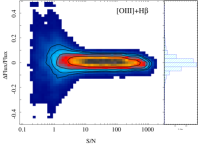
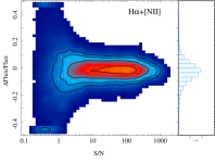
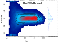
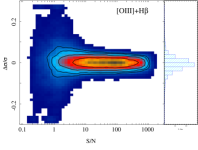
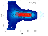
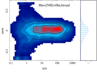
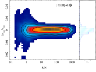
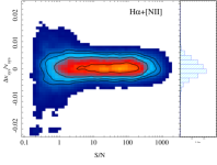
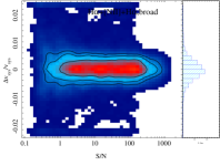
Figure 11: Relative difference between the recovered and the simulated parameters of the emission lines (top: flux intensity, middle: velocity dispersion, and bottom: velocity) for the three sets of simulated emission lines corresponding to [O iii]+H$\beta$ (left panels), [N ii]+H$\alpha$ (central panels), and this later one with an additional broad component for H$\alpha$ (right panels), as a function of the signal-to-noise of the emission lines. For each panel the contours corresponds to the density of points, with the first contour encircling the 95% of the points, and each consecutive contour encircling a 15% less number of points.

0.3.3 Accuracy of the properties of the emission lines

Following a similar philosophy, we create a set of simulations in order to derive the accuracy and precision of the recovery of the properties of the emission lines. The first set of simulations was created assuming purely poissonian noise, and without taking into account the possible effects of the imperfect subtraction of the underlying stellar population, and other sources of non poissonian noise. We simulated three different systems of emission lines within this set of simulations: (i) H$\beta$ and [O iii]$\lambda$4959,5007, with a flux intensity of 100, 66, and 22 10^-16 erg s^-1 cm^-2 Å^-1, respectively, and covering the wavelength range 4800-5050 Å, in the rest-frame; (ii) H$\alpha$, [N ii]$\lambda$6548,6583, and [S ii]$\lambda$6717,6731, with a flux intensity of 100, 66, 22, 25, and 25 10^-16 erg s^-1 cm^-2 Å^-1, respectively, covering a wavelength range 6400-6900Å; and (iii) the same emission lines included in the previous simulation plus a broad H$\alpha$ component, covering the same wavelength range.

All the emission lines, except the broad component included in the last set, were simulated assuming the same range of velocity dispersion used in the simulations of the stellar populations, $\sigma=$2.5Å and 7.5Å ($\sigma_{v}\sim 100-400$ km/s). The velocity dispersion is then selected randomly within this range. Therefore, while in case (i) the emission lines are always deblended, in case (ii) there are cases in which the emission lines are deblended, but in many other cases they show different levels of blending. Finally, in case (iii) the narrow emission lines present the same degree of blending than in case (ii), but in all the cases they are blended with the broad emission line. This affects the accuracy and precision of the recovered emission line properties. For the broad component included in case (iii) we consider a range of velocity dispersion $\sigma=32.5-37.5$ Å ($\sigma_{v}\sim 1500-1700$ km/s).

The velocity was randomly selected around $6000\pm 500$ km/s, for the narrow emission lines. The broad component is randomly redshifted by 200 km/s from this velocity, which is a typical situation in the case of broad components generated by either outflows or type one AGNs. The emission line spectra were sampled with a pixel scale of 2Å/pix, similar to the one provided by the CALIFA V500 data set. The results can be extrapolated to other instrumental configurations taking into account the ratio between the velocity dispersion and the size of the sampling pixel. The effect of the instrumental configuration has not been taken into account. It affects mostly the recovering of the physical velocity dispersion, which is a quadratic subtraction of the instrumental one from the measured dispersion. Therefore, it basically depends on this later parameter, although not in a linear way.

Table 3: Results of the simulations: Emission lines.

Results for the [O iii]+H$\beta$ emission lines
S/N	$\Delta$Flux/Flux	$\Delta$$\sigma_{v}$/$\sigma_{v}$	10$\Delta$vsys/vsys1
$<$3	0.01 $\pm$0.15	0.00 $\pm$0.11	0.00 $\pm$0.06
3$-$10	0.00 $\pm$0.05	0.00 $\pm$0.04	0.00 $\pm$0.03
10$-$100	0.01 $\pm$0.04	$-$0.01 $\pm$0.02	0.00 $\pm$0.02
$>$100	$-$0.01 $\pm$0.03	$-$0.01 $\pm$0.02	0.00 $\pm$0.02
Results for the [N ii]+H$\alpha$ emission lines
S/N	$\Delta$Flux/Flux	$\Delta$$\sigma_{v}$/$\sigma_{v}$	10$\Delta$vsys/vsys
$<$3	$-$0.02 $\pm$0.24	0.01 $\pm$0.14	0.00 $\pm$0.09
3$-$10	$-$0.02 $\pm$0.08	0.01 $\pm$0.05	0.00 $\pm$0.04
10$-$100	$-$0.03 $\pm$0.07	0.00 $\pm$0.04	0.00 $\pm$0.03
$>$100	$-$0.03 $\pm$0.05	$-$0.01 $\pm$0.04	0.00 $\pm$0.03
Results for the [N ii]+H$\alpha$+H$\alpha,broad$ emission lines
S/N	$\Delta$Flux/Flux	$\Delta$$\sigma_{v}$/$\sigma_{v}$	10$\Delta$vsys/vsys
$<$3	$-$0.01 $\pm$0.17	0.00 $\pm$0.09	0.00 $\pm$0.08
3$-$10	$-$0.01 $\pm$0.10	0.00 $\pm$0.06	0.00 $\pm$0.08
10$-$100	$-$0.01 $\pm$0.09	0.00 $\pm$0.05	0.00 $\pm$0.07
$>$100	$-$0.01 $\pm$0.07	0.00 $\pm$0.04	0.00 $\pm$0.05

(1) $\Delta$v_sys is multiplied by ten to show it at the same scale of the other two parameters.

Figure 11 shows the comparison between the recovered and simulated parameters for three sets of simulated emission lines as a function of the signal-to-noise ratio of the emission lines. The S/N is estimated as the ratio between the peak intensity of the emission line and the noise level included in the simulated spectrum. As expected there is a clear dependence with S/N (for S/N$<$10), with the worst recovered parameters corresponding to the lower S/N emission lines. For large S/N values ($>$20) there is almost no dependence of the uncertainty with the S/N. There is also a clear difference between the three sets of simulations, with the better precision corresponding to case (i), and the worst to case (iii). This is not an effect of the signal-to-noise, since in case (i) and case (ii) all the emission lines have the same integrated fluxes and a similar flux density per spectral pixel for a fixed dispersion.

A summary of these results is included in Table 3. For each set of simulated emission lines, it lists the mean and standard deviation of the relative difference between the recovered and simulated parameters for different ranges of signal-to-noise ratio. The program is able to recover the intensity of the emission lines with a precision better than $\sim$10% for weak emission lines (S/N$\sim$3-10), in all the cases. The precision becomes worse, $\sim$20%, for emission lines swimming in the noise, although the accuracy is equally good. However, at this low S/N values the systematic effects (in the subtraction of the underlying stellar population and other sources of non Poissonian noise not considered in this simulation) will dominate, and therefore this precision should be considered as an upper limit. It is interesting to notice that although the precision increases towards higher signal-to-noise ratios, it never gets better than $\sim$3%, at least for the highest S/N ratios explored in this simulations. We consider that this threshold is related to the fact that we fit together the intensity, velocity, and velocity dispersion, and their derivation is somehow correlated. Therefore, the S/N of the integrated flux alone may not be a good parameter to characterize how well the emission lines are detected.

The velocity and velocity dispersion are also well recovered. In the case of the velocity dispersion it has a similar precision as the emission line intensity; it is recovered with a precision better than 10% in almost all the simulated spectra. The best precision for this parameter is $\sim$2%, even for high S/N spectra. Finally, the velocity is recovered with a very high precision, $\sim$10 times better than the other two parameters. The precision ranges $\sim$12–54 km/s at the average redshift of the simulated spectra. This precision is between two and ten times better than the simulated velocity dispersion. These simulations confirm a widely accepted result indicating that the velocity derived using emission lines could be recovered with a precision as good as a few per cent of the velocity dispersion of the emission lines (typically 10%).

As already noticed, the precision of the emission lines parameters recovered is different for each set of simulations, being, in general, worst for the simulations with blended emission lines. The degradation of the precision could be as bad as two times the precision if the emission lines are not blended.

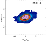
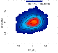
Figure 12: Relative difference between the recovered and the simulated intensity of the emission lines for the three sets of simulated emission lines corresponding to [O iii]+H$\beta$ (left panel), [N ii]+H$\alpha$ (central panel), and this later one with an additional broad component for H$\alpha$ (right panels), as a function of the relative difference between the recovered and the simulated velocity dispersion of the corresponding emission lines. For each panel the contours correspond to the density of points, with the first contour encircling the 95% of the points, and each consecutive contour encircling a 15% less number of points.

Interdependence of the accuracy between parameters

As indicated before, the precision in the estimation of one of the parameters may affect the accuracy with which others are recovered. In particular, the velocity dispersion could affect the recovered flux intensity, since this parameter is an integral that depends on the former one. Figure 12 shows the relative accuracy of the recovered flux intensity as a function of the accuracy of the recovered velocity dispersion for the three sets of simulations described before. In all three cases the distributions show a cloud of points with a dispersion of the order of $\pm$0.1$\Delta_{par}/par$. However, it is clear that the distribution is broader and more roundish for the simulations including blended emission lines than for the simulations including only well resolved emission lines (left panel). This is a consequence of the larger errors/inaccuracies in the derivation of both the flux intensity and the velocity dispersion for the blended emission lines, as shown in Section 0.3.3. In this analysis we used all the simulations described before irrespectively of the S/N. We repeated the analysis for different S/N ranges without significant differences. Only for the very low S/N ($<$10) regime we found a broadening of the distribution, but the main trends hold.

There is a clear trend between both relative differences, that are stronger for the simulations with un-blended emission lines, with a correlation coefficient $r=$0.41 ($p>99.99\%$ of not being produced by a random distribution of the data). This indicates that the bias introduced in the estimation of the flux intensity by the inaccuracy in the derivation of the emission lines is stronger for clearly blended emission lines. However it is not a dominant factor in the error budget, in the signal-to-noise range of our simulations.

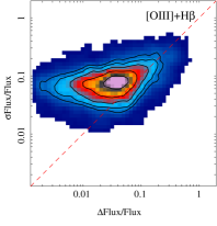
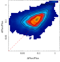
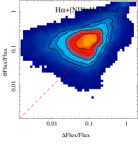
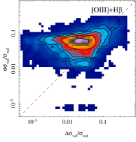
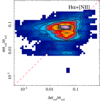
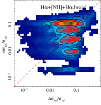
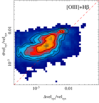
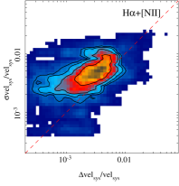
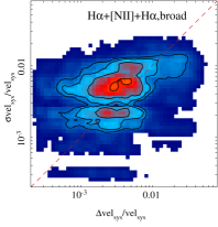
Figure 13: Relative error estimated for the emission lines recovered parameters (top: flux intensity, middle: velocity dispersion, and bottom: velocity) for the three sets of simulated emission lines corresponding to [O iii]+H$\beta$ (left panel), [N ii]+H$\alpha$ (central panel), and this later one with an additional broad component for H$\alpha$ (right panels), as a function of the relative difference between the recovered and the simulated value of this parameter for the corresponding emission line. For each panel the contours correspond to the density of points, with the first contour encircling 95% of the points, and each consecutive contour encircling a 15% less number of points. The red dashed line in each panel corresponds to the one-to-one relation.

Accuracy on the estimated errors for the emission lines

As in the analysis of the stellar population, it is important to determine whether the estimated errors are representative of the real ones. Following the previous analysis, we compare for each emission line in each of the three simulated datasets the estimated error with the real ones, i.e., the absolute difference between the value recovered and the simulated (input) one. Figure 13 shows the results of this comparison.

As shown in previous sections, in general, the real error in the derivation of the parameters is larger for the simulations including blended emission lines than in those including only un-blended ones. For the flux intensity, the estimated errors seem to be a good representation of the real ones for real errors larger than $\sim$4-5%. For errors smaller than this value the program seems to overestimate the errors, and derive a minimum value of $\sim$5%, regardless of the real difference between the input and output parameters. However, since in most simulations it seems that the emission intensities cannot be recovered with a precision better than a few percent, this lower-limit still seems reasonable.

For the velocity dispersion the estimated errors seem to be of the same order of the real ones, at least for the simulations that do not include broad emission lines. In general, the errors seem to be slightly overestimated, with a similar trend towards a minimum value of the error around $\sim$5%. For the simulations including broad emission lines the estimation of the error shows a wide scatter, with a clear underestimation of the error in many cases. We have investigated in detail, and the larger variations in the estimation of the error correspond to the broad emission line component included in this simulation. It is interesting to note that, in any case, the dispersion seems to be well recovered (see Fig. 11), but for broad emission lines the program tends to underestimate the errors.

Finally, the estimated errors for the velocities are an order of magnitude lower than the errors derived for the other two parameters. They are just slightly overestimated compared to the real difference between the input and recovered velocities, being a good representation of the real errors in general. As in previous cases, the estimated errors are more accurate for the simulations including only narrow emission lines.

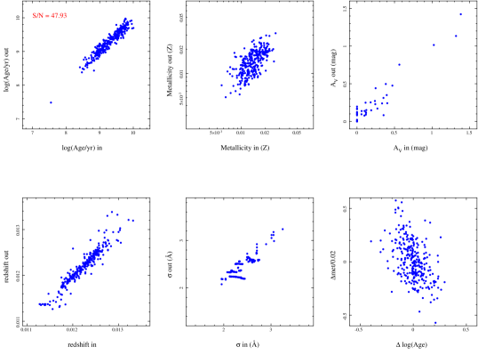
Figure 14: Results from the simulations based on the CALIFA V500 data cube of NGC 2916. Each panel shows, from left to right and from top to bottom, the comparison between the input luminosity-weighted age, metallicity, dust attenuation, redshift, and velocity dispersion with the values recovered by our fitting technique. The results are presented for gsd156 template. The final bottom-right panel illustrates the degeneracy between the recovered age and metallicity, showing a comparison between the input-output differences for both parameters.

0.3.4 Simulations using real data

So far we have estimated the accuracy and precision of the parameters using simulations that only take into account the Poissonian noise. To investigate further the precision in the derivation of the parameters we require to take into account all the different sources of error that are included in real data.

For these particular simulations we use the data sets provided by the CALIFA survey. In particular, we adopted the V500 data cube corresponding to NGC 2916, an Sbc galaxy at $z\sim$0.01244, that is an average galaxy in this survey. This data cube comprises 78$\times$72 individual spectra, of which $\sim$2500 contain data and the rest are out of the original hexagonal pattern of the instrument. We need to remark that the simulations do not depend on the particular galaxy selected. We used this one since it presents both strong and weak emission lines within the FoV of the data cube, and therefore they cover a wide range of signal-to-noise ratios.

The simulations are created using as input the results from the fitting using Pipe3D over this particular dataset. The analysis with Pipe3D will be detailed in forthcoming articles of this series, although some examples of the data products have been presented already elsewhere (Sánchez et al., 2013). For the purpose of this study we should know that the pipeline performs a spatial binning over the data cube, aggregating adjacent spaxels based on their difference in relative intensity (at a reference wavelength); it provides a final row-stacked spectra (RSS) comprising $\sim$500-1000 individual spectra with an increased signal-to-noise (in the continuum) with respect to the individual spaxels. Finally, each of the individual spectra is analyzed using the current version of FIT3D to provide all the data products regarding the stellar population and the emission lines described in previous sections. In this particular analysis we adopted the results derived using the gsd156 stellar library template.

Table 4: Results of the simulations: simulated NGC 2916 data cube.

S/N	$\Delta$Age/Age	$\Delta$Z/Z	$\Delta$AV1	$\Delta$vsys1	$\Delta$$\sigma_{v}$1	$r_{cor}$2
47.9	0.00 $\pm$0.11	0.00  $\pm$0.12	0.01 $\pm$0.08	-10.8 $\pm$ 40.7	2.7 $\pm$ 7.3	0.47
19.5	-0.06 $\pm$0.26	-0.01  $\pm$0.14	0.07 $\pm$0.28	-57.3 $\pm$144.7	4.6 $\pm$ 7.8	0.08
11.8	-0.09 $\pm$0.37	-0.04  $\pm$0.14	0.14 $\pm$0.48	-57.4 $\pm$166.1	6.6 $\pm$ 3.3	0.35
5.4	-0.31 $\pm$0.38	-0.03  $\pm$0.11	0.66 $\pm$0.58	-186.0 $\pm$218.5	7.4 $\pm$ 7.4	0.26

The resulting star formation history, stellar kinematics, stellar dust attenuation, and the corresponding data products of the emission lines (intensity, velocity, and velocity dispersion) can be used as input parameters for a simulation with more realistic parameters. For each spatial bin we create a spectrum with a model stellar continuum and a model set of emission lines, using as input the output of the fit over the real data. Then, we renormalize the flux in each individual spaxel within each bin following the relative contribution of the flux to the bin by this spaxel in the original data. In this way we have a realistic model data cube with the same spatial distribution of the stellar population and ionized gas as the real data.

Then, we use the residuals from the fitting process over the observed data cube to generate a realistic distribution of the noise, that comprises not only the Poissonian noise, but any other source of error. To do so, we use the residual data cube obtained from the analysis with FIT3D, and, for each spaxel at each wavelength, we coadd a random value within a range plus-minus the median of the absolute value of the noise distribution within a box of $\pm$3$\arcsec$. In this way we respect the amplitude of the real noise at each wavelength and at each position within the data cube, excluding the peaks in the noise distribution (like the ones produced by cosmic-rays or inaccuracies in the sky subtraction). We should clarify that this derivation of the noise does not follow either a Gaussian or a square distribution.

We then apply the same spatial segmentation to extract the RSS-spectra at the same spatial locations than in the case of the original data cube. After that, we process the spectra using the same fitting routines to recover both the properties of the stellar population and emission lines. We adopted the same stellar population library for the analysis, for a better comparison between the input and output parameters. We analyzed four sets of emission lines, with coupled kinematics, as described in Sec. 0.2.4. Those emission lines are analyzed in four wavelength ranges: (1) [O ii]$\lambda$3727 (3700-3750Å); (2) H$\beta$ and [O iii]$\lambda$4959,5007 (4800-5050Å); (3) H$\alpha$ and [N ii]$\lambda$6548,6583 (6680-6770); and (4) [S ii]$\lambda$6717,6731. Altogether, they comprise more than 5000 individual emission lines, with different line intensities, at a wide range of wavelengths. Therefore, they are affected in a different way by the imperfect subtraction of the underlying stellar population and the wavelength dependence depth of the data. All the emission lines considered here are deblended at the spectral resolution of the V500 CALIFA data, however, some of them could be affected by the wing of the adjacent emission lines, in particular the doublet [S ii]$\lambda$6717,6731.

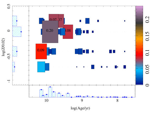
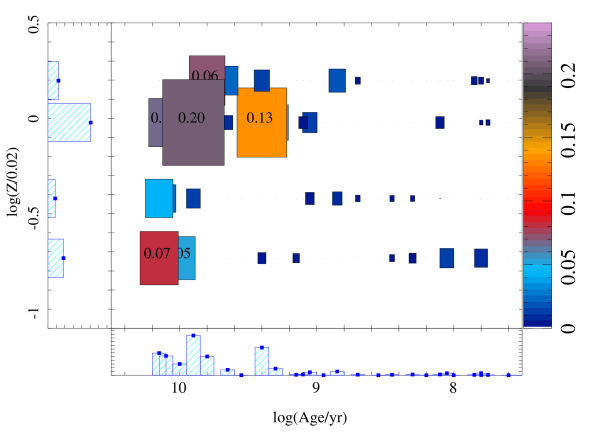
Figure 15: Top panel: Coefficient distribution along the age-metallicity grid derived from the analysis using FIT3D of the central 5$\arcsec$ diameter aperture spectrum extracted from the CALIFA V500 data cube of NGC 2916, used as input coefficients in the simulated spectra described in the text. Bottom panel: Similar distribution corresponding to the recovered coefficients for the simulated spectrum, resulting from the fitting procedure. All the symbols are similar to those described in Fig. 9.

Accuracy of the properties recovered for the stellar populations

Figure 14 shows the results of comparing the data products derived for the stellar populations as a function of the corresponding input/simulated values, for spectra with S/N higher than 20. As in the case of Fig. 8, it demonstrates that there is a good correspondence between the input and the recovered parameters, with a clear one-to-one correlation in all the cases. A more quantitative comparison is included in Table 4, that shows the average S/N and the difference between the input and the recovered values, for different ranges of S/N. Despite the different procedure adopted, the results are very similar to the ones shown in Tables 1 and 2. For spectra with a S/N higher than $\sim$20, most parameters are recovered with a precision of $\sim$10%. In the case of the velocity it is an order of magnitude better. It is interesting to note that the velocity is recovered with a better precision when using a more realistic SFH than a purely simulated one.

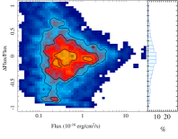
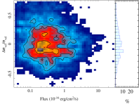
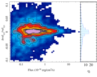
Figure 16: Relative difference between the recovered and input values for the parameter analyzed for the emission lines (left: flux intensity, center: velocity dispersion and right: velocity) for the simulation based on the CALIFA V500 data of NGC 2916 as a function of the emission lines flux intensities. For each panel the colored images and contours correspond to the density of points, with the first contour encircling 95% of the points, and each consecutive contour encircling a 15% less number of points.

As in the previous cases, we explore the possible effect of the age-metallicity degeneracy in these more realistic simulations. The last panel of Fig. 14 shows a comparison of the offset between the output and input ages, and the offset between the output and input metallicities of the stellar populations. There is a weak trend between the two offsets, in the expected direction induced by this degeneracy. The strength of this degeneracy is parametrized by the correlation coefficient between the two parameters, listed in Table 4. The trend is weak, and affects relatively more to metallicity than to age. This is expected since the relative error in the derivation of age is always lower than the error in the derivation of metallicity. As expected, this degeneracy, that is a systematic effect, is enhanced by the S/N of the data. The effect is stronger for the more metal poor stellar populations, since the offset ranges between $\pm$0.5 Z/Z$\odot$, i.e., $\Delta Z=$$\pm$0.01. For the metal rich its effect is marginal, but for the stellar populations with sub-solar abundances it could bias the result by a factor 2 or more.

We note here that the degeneracy and the range of offsets between the input and output parameters is larger than the values reported in previous studies (e.g. Ocvirk et al., 2006; Sánchez-Blázquez et al., 2011), as we indicated before. Although they are of same order as the ones reported by more recent simulations (e.g. Cid Fernandes et al., 2014). Maybe the reason for this disagreement is that, although in the previous cases a full SFH was considered and reasonable chemical enrichment processes, they did not explore a wide range of possible uncertainties in the dust attenuation and the velocity dispersion, although they have a hint of its effect (e.g., Fig. B3 of Sánchez-Blázquez et al., 2011).

Figure 15 shows a comparison between the input and output coefficients of the decomposition of the stellar population with the gsd156 template library for the spectra extracted using a 5$\arcsec$ diameter aperture on the real and simulated CALIFA data cube. Both distributions have a very similar pattern, with the oldest stellar population being metal poor (sub-solar metallicity), and a rapid chemical enrichment in the early epochs of the universe. The star formation history presents several bursts, with most of the stars formed in the first 1-2 Gyr of the Universe. This pattern is very similar to the one described by Pérez et al. (2013). The younger stellar populations ($<$1 Gyr) are more metal poor, which could be interpreted as a result of infall of more pristine gas into the inner regions, which could explain the remanent star formation events in the very center of this galaxy. However, it could well be that these low intensity coefficients are just a product of the noise. In any case, the code is able to recreate realistic SFHs and chemical enrichment patterns, whatever their nature.

Table 5: Results of the simulations: emission lines in the NGC 2916 data cube.

S/N	$\Delta$Flux/Flux	$\Delta$$\sigma_{v}$1	$\Delta$vsys1
30.0	-0.01$\pm$0.10	0.3$\pm$11.7	9.9$\pm$40.6
10.0	-0.05$\pm$0.16	-0.8$\pm$11.7	11.5$\pm$32.6
5.5	-0.10$\pm$0.32	-3.8$\pm$15.2	6.1$\pm$80.1
2.3	-0.15$\pm$0.45	0.9$\pm$20.7	-0.1$\pm$99.8

(1) Kinematic parameters are given in km/s.

Accuracy of the properties recovered for emission lines

Figure 16 shows the results of the comparison between the properties of the simulated emission lines and the values recovered for the simulation based on the CALIFA V500 data cube for NGC 2916. A more quantitive summary is presented in Table 5, where the average and standard deviation of the differences between the input and output values of the different parameters are presented for different ranges of signal-to-noise ratio of the emission lines. Being a realistic simulation based on a galaxy with mild emission lines, the dynamical range for the signal-to-noise is more reduced than in the case of the simulations presented in Sec. 0.3.3. The results are consistent in general. As expected, the accuracy and precision in the derivation of the different parameters is slightly lower for this simulation, which is more realistic in terms of the signal-to-noise and the propagation of the imperfect subtraction of the underlying stellar population and other sources of non-Poissonian noise. For the well detected emission lines, S/N$>$10, the flux intensity is recovered within 10-15%, the velocity dispersion is recovered within $\pm$10 km/s, and the velocity is recovered within 30-40 km/s. The precision decreases for the emission lines detected with low S/N ($<10$), and the results are unreliable for those emission lines barely detected.

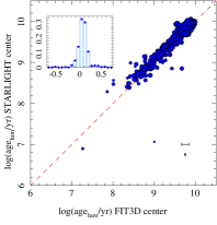
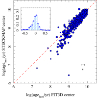
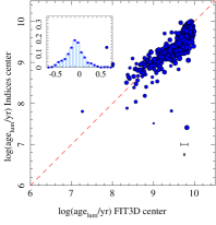
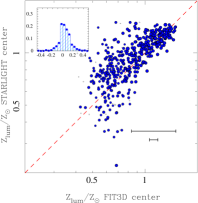
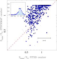
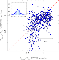
Figure 17: Comparison between the derived parameters of the stellar population for 448 central spectra extracted from the CALIFA V500 data cubes analyzed using FIT3D, Starlight, Steckmap, and absorption line indices using the same template of stellar populations. The top panels show the comparison between the luminosity-weighted ages, and the bottom panel shows the comparison between the luminosity-weighted metallicities. In all the panels the size of the symbols are inversely proportional to the S/N of the spectrum analyzed. The error bars indicate the larger and average errors in each of the parameters, as derived by FIT3D. In each panel the inset box shows the normalized histograms of the differences between the two parameters compared.

0.4 Comparison with other fitting routines

As indicated in previous sections, FIT3D is obviously not the first package developed with the aim of recovering the properties of the stellar population from optical spectra of galaxies. So far, we have illustrated how well it recovers the main parameters defining the stellar populations, based on different kinds of simulations. In the current section we explore how those parameters recovered compare to similar ones derived using other fitting tools.

We require a set of spectra with enough S/N in the continuum to minimize the effects of noise in the comparison. Therefore, we selected the central spectra extracted from the 448 CALIFA galaxies observed using the V500 setup up to September 2014, co-adding the spaxels within a diameter of 5$\arcsec$ around the peak intensity in the $V$-band. All those spectra have a S/N$>$50 per spectral pixel, as shown in Sánchez et al. (2012b). The wide range of galaxy masses and morphologies covered by CALIFA guarantees that we explore a wide range of stellar populations with those spectra. We analyzed them with FIT3D, using the gsd156 template library, and the procedures described in the previous sections.

Using the same data set and the same library we applied, in addition to FIT3D, (i) starlight (Cid Fernandes et al., 2005), following the prescriptions described in Cid Fernandes et al. (2013), (ii) Steckmap (Ocvirk et al., 2006), following the prescriptions described in Sánchez-Blázquez et al. (2011), Sánchez-Blázquez et al. (2014a), and Sánchez-Blázquez et al. (2014b), and (iii) the analysis based on the study of the absorption line indices described in Sánchez et al. (2007b) and Sánchez et al. (2011). In summary, after subtracting the emission lines, we derive for each spectra a set of stellar indices (H$\delta$, H$\beta$, Mg$b$, Fe5270, Fe5335, and D4000), and we estimate the ages and metallicities based on a comparison with the expected values for each pair of indices with the corresponding ones for the same stellar template, using the rmodel program Cardiel et al. (2003). It is beyond the scope of this article to describe in detail the different codes, however, we should note that they rely on very different assumptions and inversion algorithms. In essence, starlight is more similar to FIT3D since it does a pseudo-random exploration of the parameter space based on a Markov chain method. However, as indicated before FIT3D does not adopt the Markov chain, and performs a MC realization process and a linear inversion to derive the weights of the stellar decomposition. None of these two codes makes any a priori assumption on the shape of the star-formation history. On the contrary, Steckmap performs a derivation of the star formation history using a peak-to-peak fitting algorithm (Ocvirk et al., 2006), that allows to introduce a Bayesian prior on the shape of the star formation history (e.g. Sánchez-Blázquez et al., 2014a). Finally, the analysis of the stellar indices presents larger uncertainties for a similar S/N level, as demonstrated by Sánchez-Blázquez et al. (2011). However, it is the method that requires less number of assumptions and computationally is the simplest: It is a derivation, not a fitting, and it compares with a single SSP model, not with a combination of them. An additional difference is that both the indices and Steckmap do not take into account the effects of the dust attenuation, since they remove the continuum (which may have additional advantages if the spectrophotometric calibration has problems of any kind). In the case of the line indices any dust attenuation affects the age and metallicity derivation, since a priori it is assumed that it may affect D4000. Despite all these differences, the main aim of the different methods is to provide with a realistic estimation of the parameters that define the properties of the stellar population.

Figure 17 illustrates the results of this comparison. It shows the derived luminosity-weighted ages and metallicities for the different spectra as derived by FIT3D, starlight, Steckmap, and the analysis of the stellar indices. The correspondence between the luminosity-weighted ages is very good for all, starlight ($\Delta age=-$0.06$\pm$0.15 dex), Steckmap ($\Delta age=$0.03$\pm$0.22 dex), and the stellar indices ($\Delta age=$0.06$\pm$0.15 dex). However, the distribution is compatible with a one-to-one relation taking into account the estimated errors only for the comparison with starlight, with a $\chi^{2}/\nu=$1.14. The largest discrepancies correspond to the spectra with the youngest stellar populations, in particular for Steckmap. These populations are also the ones that present the strongest dust attenuations, and maybe this is the reason for this discrepancy. In more detail, the agreement between the ages seems to be better with starlight, than with Steckmap, that presents a systematic difference towards younger stellar populations than FIT3D.

The agreement between the metallicities is clearly better for starlight ($\Delta met=-$0.03$\pm$0.10 dex), than for the other two methods, Steckmap ($\Delta met=$0.03$\pm$0.22 dex), and stellar indices ($\Delta met=$0.10$\pm$0.27 dex), when compared with FIT3D. Indeed, the distribution is compatible with a one-to-one relation taking into account the estimated errors only for the comparison with starlight, with a $\chi^{2}/\nu=$1.08. In particular, in the range of more metal rich stellar populations, for which Steckmap collapses the values towards the highest metallicities in the SSP libraries. This may reflect the similarities in the procedure between FIT3D and starlight, and the differences between both of them and Steckmap. In the case of the stellar indices the agreement is better for the range of more metal rich stellar populations, for which the absorptions sensible to the metallicity are more prominent.

As a sanity check we perform the same comparison for the values derived between both starlight and Steckmap, and we find similar results. The dispersion in the differences between the parameters derived is $\Delta age=$0.10$\pm$0.26 dex, and $\Delta met=-$0.10$\pm$0.14 dex, respectively, confirming the trend described when comparing both procedures with FIT3D. Curiously, the values derived with FIT3D seem to correspond somehow to the average/intermediate values derived by both methods. If the discrepancies were dominated by systematic effects or differences between the three methods, this should not be the case (appart from the effect in the metallicity when comparing with Steckmap). For the stellar indices we found that the differences in ages and metallicities correlate with dust attenuation, as a clear indication that this method tries to compensate the effects of dust by assuming an older and more metal rich stellar population.

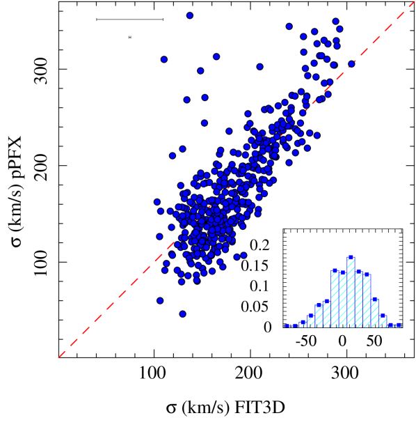
Figure 18: Comparison between the stellar velocity dispersion derived for 448 central spectra extracted from the CALIFA V500 data cubes analyzed using FIT3D and pPFX. The inset box shows the normalized histograms of the differences between the two velocity dispersion measurements.

0.4.1 Comparison of the stellar velocity dispersion

FIT3D provides the main parameters of the stellar populations, including the stellar kinematics. In general, the stellar velocity is very well recovered by most of the stellar population analysis procedures with a good accuracy and precision. However, the stellar velocity dispersion is not recovered equally well, mostly due to the degeneracy between velocity dispersion and metallicity (e.g. Sánchez-Blázquez et al., 2011).

It is widely accepted that one of the best procedures to analyze the stellar kinematics is pPXF (Cappellari & Emsellem, 2004b). This routine allows to recover the line-of-sight velocity distribution (LOSVD) from absorption line spectra with high accuracy, allowing to model it not only with a simple Gaussian, characterized by its velocity and velocity dispersion, but with more complex profiles for the LOSVD, including asymmetries characterized by Hermite functions and/or multiple Gaussian-like velocity components. This is the reason why it is widely used in stellar population analyses, even when additional tools are needed to derive the other main properties of those stellar populations (e.g. Sánchez-Blázquez et al., 2014a, b). The current capabilities of pPXF regarding the analysis of the stellar kinematics are far beyond the procedures implemented in the improved version of FIT3D. However, it is worth comparing the parameters derived, in particular the stellar velocity dispersion, to illustrate the precision of our current estimations.

Figure 18 shows the comparison between the stellar velocity dispersion derived using FIT3D with the one derived using pPXF for the set of spectra described in Sec. 0.4. There is a very good agreement between the estimations done by both procedures ($\Delta\sigma=-$9.8$\pm$36.7 km/s), with a difference compatible with the expected precision for the given spectral resolution ($R\sim$850 Sánchez et al., 2012b). Therefore, despite the fact that the current version of FIT3D is not optimized for the analysis of the kinematic properties of the stellar populations, it provides an accurate estimation of stellar velocity dispersion.

In summary, we can conclude that parameters of the stellar populations derived with FIT3D are consistent with those provided by other algorithms, with the difference that this new algorithm provides a reliable estimation of the errors of those parameters.

0.5 Summary and conclusions

In this article we present a new version of FIT3D, a package developed to analyze the optical spectra of galaxies, in order to derive the main properties of their stellar population and the ionized gas. FIT3D implements a new MC iteration method that provides not only the numerical values of the parameters, but also an estimation of their errors. In this regard the procedure is a substantial modification of the previous version of the package.

The main results of this study are the following:

• The fitting routine is confronted with simulations that demonstrate its ability to recover the properties of the underlying stellar population and the emission lines. We found that the algorithm is able to recover the luminosity weighted ages and metallicities with a precision of $\sim$0.2 dex for spectra with a S/N per pixel better than $\sim$50, for most of the stellar templates analyzed in the simulations. We found systematic differences/offsets in the recovered parameters. However, they are sub-dominant for the individual realizations, and only significant in an statistical way. We recover the well known age - metallicity - dust attenuation degeneracies. In general, the degeneracies are of the order of the precision in the parameters recovered. The use of different templates with different spectral resolutions and coverage of the parameter space affects the accuracy and precision of the parameters recovered in a similar way as a decrease of the S/N. In this regard, it is recommended to use simulations ad hoc in order to determine which stellar templates are the optimal for each particular data set. In general we cannot recover the luminosity-weighted age, metallicity, and dust attenuation with a precision better than $\sim$0.1 dex, even for the highest signal-to-noise.

• The algorithm is not tuned to derive an accurate/precise stellar kinematics. However, it provides a good estimation of the stellar velocity and velocity dispersion, that at a typical spectral resolution of $R\sim$1000 is never better than $\sim$25 km/s, for the highest S/N explored. The current implemented approach to derive the kinematics introduces a systematic effect in the profile of the absorption lines subtracted. This is translated to an unrealistic emission that is at most of the order of EW(H$\alpha$)$\sim$0.4Å, far below the typical detection limit for most of spectroscopic surveys (e.g., Gomes et al., in prep., Papaderos et al., 2013).

• The program is able to recover the star formation and chemical enrichment histories for the galaxies when the signal-to-noise per pixel is large enough (S/N$>$50). The precision in the ages and metallicities recovered is better when the SFH comprises correlations between the distribution of the stellar populations than in the case of a simple distortion of a single burst of fixed age and metallicity.

• The simulations indicate that the nominal errors derived by FIT3D for the parameters that characterize the stellar populations are a factor four smaller than the estimated errors derived from the comparison of the input and estimated values for the stellar ages, metallicities, and dust attenuation.

• A detailed set of simulations allow us to determine the ability of the algorithm to recover the intensity, velocity dispersion, and velocity of the emission lines in three main cases: isolated lines, blended lines, and blended lines with an underlying broad emission line component. In general, it is possible to estimate the parameters with a precision of 0.05-0.10 dex for S/N above 3$\sigma$. As expected, the precision of the parameters derived is worse for the most blended emission lines and for the lower S/N.

• A more realistic set of simulations was created based on real spectra of a typical galaxy extracted from the CALIFA survey data cubes, by using as input for the simulations the output of the analysis of this galaxy, based on the same algorithm, and perturbed by a realistic realization of the noise, based on the residuals of the analysis described. These simulations confirm that we can recover the properties of the stellar populations with a precision of the order of $\sim$0.1 dex only for S/N$\sim$50.

• The stellar parameters derived using FIT3D are compared with similar ones derived using widely used fitting routines, like starlight and Steckmap, and with those derived using classical stellar indices, for a set of high S/N spectra extracted from the CALIFA data cubes. This comparison shows that the parameters derived by FIT3D are compatible with those derived using the other tools. In particular, there is a very good agreement in the luminosity-weighted ages for the three cases, with a typical difference of $\sim$0.15-0.22 dex. The agreement is slightly worse for the luminosity-weighted metallicities in the case of Steckmap and the stellar indices, being better for the case of starlight, with a typical difference of $\sim$0.1 dex.

In summary, we demontrate that the new algorithm implemented in FIT3D is able to recover the main properties of the stellar populations and emission lines for moderate resolution spectra of galaxies. The tool is fully prepared to analyze IFS data, and in particular is well suited for the analysis of IFU data from the major on-going surveys, like CALIFA (Sánchez et al., 2012b), MaNGA (Bundy et al., 2015), and SAMI (Croom et al., 2012). In forthcoming articles we will present a practical implementation to analyze spatially resolved spectroscopic data and a study of the possible uncertainties.