Local versus Global Biological Network Alignment

Abstract

Network alignment (NA) aims to find regions of similarities between molecular networks of different species. There exist two NA categories: local (LNA) or global (GNA). LNA finds small highly conserved network regions and produces a many-to-many node mapping. GNA finds large conserved regions and produces a one-to-one node mapping. Given the different outputs of LNA and GNA, when a new NA method is proposed, it is compared against existing methods from the same category. However, both NA categories have the same goal: to allow for transferring functional knowledge from well- to poorly-studied species between conserved network regions. So, which one to choose, LNA or GNA? To answer this, we introduce the first systematic evaluation of the two NA categories.

We introduce new measures of alignment quality that allow for fair comparison of the different LNA and GNA outputs, as such measures do not exist. We provide user-friendly software for efficient alignment evaluation that implements the new and existing measures. We evaluate prominent LNA and GNA methods on synthetic and real-world biological networks. We study the effect on alignment quality of using different interaction types and confidence levels. We find that the superiority of one NA category over the other is context-dependent. Further, when we contrast LNA and GNA in the application of learning novel protein functional knowledge, the two produce very different predictions, indicating their complementarity. Our results and software provide guidelines for future NA method development and evaluation.

1 Introduction

1.1 Motivation, background, and related work

With advancements of high throughput biotechnologies such as yeast two-hybrid (Y2H) assays [30] and affinity purification coupled to mass spectrometry (AP/MS) [9], large amounts of protein-protein interaction (PPI) data have become available [13, 2, 1]. Comparative analysis of PPI data across species is referred to as biological network alignment (NA). NA is proving to be valuable, since it can be used to transfer biological knowledge from well- to poorly-studied species, thus leading to new discoveries in evolutionary biology.

NA aims to find topologically and functionally similar (conserved) regions between PPI networks of different species [7]. Like genomic sequence alignment, NA can be local (LNA) or global (GNA). LNA aims to find small highly conserved subnetworks, irrespective of the overall similarity of compared networks (Figure 1 (a)) [25, 21, 3, 19, 11]. Since the highly conserved subnetworks can overlap, LNA results in a many-to-many mapping between nodes of the compared networks – a node can be mapped to multiple nodes from the other network. In contrast, GNA aims to maximize overall similarity of the compared networks, at the expense of suboptimal conservation in local regions (Figure 1 (b)). GNA produces a one-to-one (injective) node mapping – every node in the smaller network is mapped to exactly one unique node in the larger network [26, 18, 15, 22, 20, 28, 12, 23, 29, 27, 16, 10, 24].

NA can also be categorized as pairwise or multiple, based on how many networks it can align. See [7] for a review of pairwise and multiple NA. Here, we focus on pairwise NA.

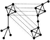
(a)          (b)

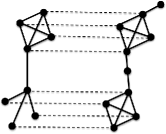
Figure 1: Illustration of (a) LNA and (b) GNA.

Given the different outputs of LNA and GNA, it is difficult to directly compare them. Hence, when a new NA method is proposed, it is compared only against existing methods from the same NA category. In this context, NA methods can be evaluated with measures of topological or biological alignment quality. An alignment is of good topological quality if it reconstructs the underlying true node mapping well (when this mapping is known) and if it conserves many edges. An alignment is of good biological quality if the mapped nodes perform similar function. LNA output is evaluated biologically but not topologically. This is because LNA outputs a many-to-many node mapping and thus it is not clear how to compute edge conservation that has been defined only for one-to-one mapping [23]. GNA is evaluated both topologically and biologically.

Despite the different output types of LNA and GNA, which makes their direct comparison difficult, the two NA categories have the same ultimate goal: to transfer functional knowledge from well- to poorly-studied species, thus redefining the traditional notion of sequence-based orthology to network-based orthology. For this reason, we introduce the first ever comparison of LNA and GNA.

1.2 Our approach and contributions

In the process of developing our novel framework for a fair comparison of LNA and GNA (Figure 2), we do the following.

1) We evaluate eight prominent LNA and GNA methods.

2) We evaluate the NA methods on both synthetic networks with known true node mapping and real-world networks with unknown true node mapping. For the latter, we explore the impact on the results of using different PPI types or PPIs of varying confidence.

3) We develop new alignment quality measures that allow for a fair comparison of LNA and GNA, since such measures do not exist. We measure both topological and biological alignment quality.

4) We study the effect on the results of using only network topological information versus including also protein sequence information into the alignment construction process.

5) Our LNA versus GNA evaluation reveals the following. When using only topological information during the alignment construction process, GNA outperforms LNA both topologically and biologically; when sequence information is also included, GNA is superior to LNA in terms of topological alignment quality, while LNA is superior to GNA in terms of biological quality. Different PPI types and confidence levels lead to consistent findings, which indicates the robustness of our approach to the choice of PPI data.

6) In addition to the thorough method evaluation, whose results provide guidelines for future NA method development, we apply the NA methods to predict novel protein functional knowledge. We find that LNA and GNA produce very different predictions, indicating their complementarity when learning new biological knowledge.

7) We provide a graphical user interface (GUI) for NA evaluation integrating the new and existing alignment quality measures.

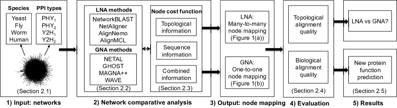
Figure 2: Summary of our LNA versus GNA evaluation framework, consisting of the following steps: (1) Input: networks from different species containing different types of PPIs. Note that for this network set, we do not know the true node mapping. Thus, we analyze an additional set of networks with known true node mapping. (2) Network comparative analysis: using prominent LNA or GNA methods (as listed) to align networks across different species. During the alignment construction process, we set each method’s node cost function (see Section 2.3) to use topological information only, sequence information only, or combined topological and sequence information. (3) Output: many-to-many node mapping for LNA or one-to-one node mapping for GNA. (4) Evaluation: measuring topological and biological quality of each alignment. (5) Results: fair comparison of LNA and GNA, and novel protein function prediction.

2 Methods

2.1 Data description

We analyze PPI networks with 1) known and 2) unknown true node mapping.

Networks with known true node mapping contain a high-confidence S. cerevisiae (yeast) PPI network with 1004 proteins and 8323 PPIs [4] and five noisy networks constructed by adding to the high-confidence network 5%, 10%, 15%, 20%, or 25% of lower-confidence PPIs from the same dataset [4]; the higher-scoring lower-confidence PPIs are added first. We align the high-confidence network with each of the noisy networks. Since all networks contain the same nodes, we know the true node mapping. The high-confidence network is an exact subgraph of each noisy yeast network. This popular evaluation test has been adopted by many existing NA studies [14, 18, 15, 17, 22, 23, 29].

Networks with unknown true node mapping are PPI data from BioGRID (downloaded in November 2014) of four species: S. cerevisiae (yeast), D. melanogaster (fly), C. elegans (worm), and H. sapiens (human). For each species, we extract four PPI networks containing different interaction types and confidence levels: 1) all physical PPIs, where each PPI is supported by at least one publication (PHY₁), 2) all physical PPIs, where each PPI is supported by at least two publications (PHY₂), 3) only yeast two-hybrid physical PPIs, where each PPI is supported by at least one publication (Y2H₁), and 4) only yeast two-hybrid physical PPIs, where each PPI is supported by at least two publications (Y2H₂). We vary the PPI type (all physical interactions, most of which are obtained by AP/MS, versus Y2H only) to test the robustness of our approach to this parameter. We vary PPI confidence levels because PPIs supported by multiple publications are more reliable than those supported by only a single publication [6]. For each network, we extract and use its largest connected component (Supplementary Section S1 and Supplementary Table S1).

2.2 Network aligners evaluated in our study

To evaluate LNA against GNA, we choose four prominent (pairwise) NA methods from each of the LNA and GNA category. More recent methods are favored since they were shown to improve upon earlier methods. Only methods with publicly available and relatively user-friendly software are considered. As a result, we choose NetworkBLAST [25], NetAligner [21], AlignNemo [3], and AlignMCL [19] from the LNA category, and we choose NETAL [20], GHOST [22], MAGNA++ [29], and WAVE [27] from the GNA category. An exception to the above guidelines is NetworkBLAST – despite being an early LNA method, NetworkBLAST still remains a popular LNA baseline. All methods are described in Supplementary Section S2 and their parameters that we use are shown in Supplementary Table S2.

2.3 Aligners’ node cost functions

All considered NA methods construct their alignments by first computing pairwise similarities between nodes from different networks via a node cost function (NCF). One can compute node similarities by accounting for: 1) topological information only (T) in order to measure how well the (extended) network neighborhoods of two nodes match, 2) sequence information only (S) in order to measure the extent of sequence conservation between the nodes, or 3) combined topological and sequence information (T&S). We study the effect on alignment quality of using only topological information versus also using sequence information in NCF.

We evaluate each aligner for each of the three above cases. The exceptions are NetworkBLAST, NetAligner, and NETAL, for the following reasons. Regarding NetworkBLAST and NetAligner, they only allow for using sequence information within NCF. The two methods require E-value scores as input and it is unclear how to convert topological information into values that are at the same scale as the E-values. Regarding NETAL, its implementation failed to run when we tried to include sequence information into its NCF. Topology- and sequence-based NCFs that we use within the different NA methods are discussed in Supplementary Section S3 and Supplementary Table S3. Given topology- and sequence-based NCFs for two nodes from different networks, we compute the nodes’ combined (T&S) NCF as the linear combination of the individual NCFs: $NCF(T\&S)=\alpha\times NCF(T)+(1-\alpha)\times NCF(S)$. We choose $\alpha=0.5$ to equally balance between T and S.

2.4 Evaluation of alignment quality

Next, we discuss measures that we use to evaluate topological (Section 2.4.1) and biological (Section 2.4.2) alignment quality. We introduce the following definitions. Let $f$ be an alignment between two graphs $G_{1}(V_{1},E_{1})$ and $G_{2}(V_{2},E_{2})$. Given a node $u$ from one graph, let $f(u)$ be the set of nodes from the other graph that are aligned under $f$ to $u$. Given a node set $V$, let $f(V)=\underset{v\in V}{\bigcup}f(v)$. Let $G^{\prime}_{1}(V^{\prime}_{1},E^{\prime}_{1})$ and $G^{\prime}_{2}(V^{\prime}_{2},E^{\prime}_{2})$ be subgraphs of $G_{1}$ and $G_{2}$ that are induced on node sets $f(V_{2})$ and $f(V_{1})$, respectively. We define conserved and non-conserved edges as follows. A conserved edge is formed by two edges from different networks such that each end node of one edge is aligned under $f$ to a unique end node of the other edge. In other words, a conserved edge is composed of two edges from different networks that are aligned under $f$ (Figure 3 (a)). A non-conserved edge is formed by an edge from one network and a pair of nodes from the other network that do not form an edge (i.e., that form a non-edge) such that each end node of the edge is aligned under $f$ to a unique node of the non-edge (Figure 3 (b)-(c)).

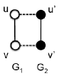
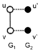
(a)          (b)          (c)

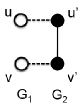
Figure 3: Illustration of conserved and non-conserved edges. (a) A conserved edge is formed by two edges $(u,v)\in G_{1}$ and $(u^{\prime},v^{\prime})\in G_{2}$ such that $u$ is aligned to $u^{\prime}$ and $v$ is aligned to $v^{\prime}$. A non-conserved edge is formed by (b) an edge $(u,v)\in G_{1}$ and a non-edge $(u^{\prime},v^{\prime})\in G_{2}$ , or by (c) a non-edge $(u,v)\in G_{1}$ and an edge $(u,v)\in G_{2}$, such that $u$ is aligned to $u^{\prime}$ and $v$ is aligned to $v^{\prime}$. Nodes of the same color come from the same network. A solid line represents an edge. Nodes linked by a dashed line are aligned under $f$.

2.4.1 Topological evaluation

First, we describe existing topological alignment quality measures, along with their drawbacks. Next, we propose new measures that are motivated by the drawbacks of the existing measures.

Existing measures. Recall that intuitively an alignment is of high topological quality if it reconstructs the underlying true node mapping well (when such mapping is known) and if it conserves many edges.

To evaluate how well an alignment reconstructs the true node mapping, node correctness ($NC$) has been widely used [14, 18, 15]. To date, $NC$ has been defined only for GNA, as the fraction of nodes from the smaller network that are correctly aligned (under injective mapping $f$) to nodes from the larger network with respect to the true node mapping. The reason that $NC$ has not been defined for LNA is that with LNA, a node from the smaller network can be mapped to multiple nodes from the larger network, and thus, it is not clear how to measure the percentage of nodes from the smaller network that are correctly aligned. Hence, below, we generalize $NC$ for both LNA and GNA. $NC$ can only be used when the true node mapping is known.

To measure how well edges are conserved under an alignment, three measures have been used to date: edge correctness ($EC$) [14], induced conserved structure ($ICS$) [22], and symmetric substructure score ($S^{3}$) [23]. $S^{3}$ has been shown to be superior to $EC$ and $ICS$, since intuitively it not only penalizes alignments from sparse graph regions to dense graph regions (as $EC$ does), but also, it penalizes alignments from dense graph regions to sparse graph regions (as $ICS$ does). Hence, we only focus on $S^{3}$. Like $NC$, $S^{3}$ has been only defined in the context of GNA, as $\frac{|E^{*}_{1}|}{|E_{1}|+|E^{{}^{\prime}}_{2}|-|E^{*}_{1}|}$, where $|E^{*}_{1}|$ is the number of edges from $G_{1}$ that are conserved by $f$ (in this case, $G_{1}$ is the smaller of the two networks in terms of the number of nodes). The reason that $S^{3}$ has not been defined for LNA is that with LNA that allows for many-to-many node mapping, it is not clear how to count conserved edges, since an edge from one network could be aligned to multiple edges from the other network. Hence, below, we generalize $S^{3}$ to both LNA and GNA.

New measures. To address the above issues, we propose new measures.

1) Precision, recall, and F-score of node correctness (P-NC, R-NC, and F-NC, respectively). NC, defined only for GNA, measures how well an alignment reconstructs the true node mapping. As such, NC evaluates the precision of the alignment – the percentage of the aligned node pairs that are also present in the true node mapping. However, the corresponding recall – the percentage of all node pairs from the true node mapping that are aligned under $f$ – is not measured explicitly. This is because for GNA, recall has the same value as precision. On the other hand, with LNA, precision and recall could have different values. In order to generalize $NC$ for both GNA and LNA, we propose P-NC, R-NC, and F-NC. Let $M$ be the set of node pairs that are mapped under the true node mapping. Let $N$ be the set of node pairs that are aligned under $f$. P-NC is defined as $\frac{|M\cap N|}{|M|}$. R-NC is defined as $\frac{|M\cap N|}{|N|}$. F-NC, which combines P-NC and R-NC, is the harmonic mean of the two individual measures. Like $NC$, our three new measures can only be used when the true node mapping is known.

2) Generalized S³ (GS³). To generalize S³ for both GNA and LNA, we propose GS³ to count edge conservation under $f$, independent on whether $f$ is injective or many-to-many. We define GS³ as the percentage of conserved edges out of the total of both conserved and non-conserved edges. Let $N_{c}$ and $N_{n}$ be the number of conserved and non-conserved edges, respectively. That is, $N_{c}=\sum_{uv\in E^{\prime}_{1}}|\{(u^{\prime},v^{\prime})|u^{\prime}\in f(u),v^{\prime}\in f(v),(u^{\prime},v^{\prime})\in E^{\prime}_{2}\}|$. $N_{n}$ is the sum of $N^{1}_{n}$ (i.e., the number of non-conserved edges formed by aligning an edge from $G_{1}$ and a non-edge from $G_{2}$; Figure 3b)) and $N^{2}_{n}$ (i.e., the number of non-conserved edges formed by aligning a non-edge from $G_{1}$ and an edge from $G_{2}$; Figure 3c)). In other words, $N_{n}=N^{1}_{n}+N^{2}_{n}$, where $N^{1}_{n}$ and $N^{2}_{n}$ can be computed as follows. $N^{1}_{n}=N^{1^{\prime}}_{n}-N_{c}$ and $N^{2}_{n}=N^{2^{\prime}}_{n}-N_{c}$, where $N^{1^{\prime}}_{n}=\sum_{uv\in E^{{}^{\prime}}_{1}}|\{(u^{\prime},v^{\prime})|u^{\prime}\in f(u),v^{\prime}\in f(v),u^{\prime}\neq v^{\prime}\}|$ and $N^{2^{\prime}}_{n}=\sum_{u^{\prime}v^{\prime}\in E^{{}^{\prime}}_{2}}|\{(u,v)|u\in f(u^{\prime}),v\in f(v^{\prime}),u\neq v\}|$. Then, $GS^{3}$ can be computed as: $GS^{3}=\frac{N_{c}}{N_{c}+N_{n}}=\frac{N_{c}}{N_{c}+N^{1}_{n}+N^{2}_{n}}=\frac{N_{c}}{N_{c}+(N^{1^{\prime}}_{n}-N_{c})+(N^{2^{\prime}}_{n}-N_{c})}=\frac{N_{c}}{N^{1^{\prime}}_{n}+N^{2^{\prime}}_{n}-N_{c}}$. Clearly, for GNA, this formula for $GS^{3}$ is $S^{3}$ itself.

3) NCV combined with GS³ (NCV-GS³). Recall that GS³ measures how well edges are conserved between $G^{\prime}_{1}$ and $G^{\prime}_{2}$. LNA could produce small conserved subgraphs, which could result in high $GS^{3}$ score. This would mistakenly imply high alignment quality if we only rely on $GS^{3}$. But if we adopt an additional criterion of what a good alignment is, namely high node coverage (NCV), which is the percentage of nodes from $G_{1}$ and $G_{2}$ that are also in $G^{\prime}_{1}$ and $G^{\prime}_{2}$ (i.e., $\frac{|V^{{}^{\prime}}_{1}|+|V^{{}^{\prime}}_{2}|}{|V_{1}|+|V_{2}|}$), then small conserved subgraphs with high $GS^{3}$ would actually have low alignment quality with respect to NCV. Thus, we combine NCV and GS³ into NCV-G$S^{3}$ to get a more complete picture of the actual alignment quality. We define NCV-G$S^{3}$ as the geometric mean of the two individual measures, because we want at least one low alignment quality score to imply low combined score.

2.4.2 Biological evaluation

To evaluate the biological quality of LNA and GNA, we use Gene Ontology (GO) correctness [14, 15, 20] and the accuracy of known protein function prediction [25, 15, 22]. Many GO annotations are obtained via sequence comparison [5]. Using such data to evaluate alignments of NA methods that already use sequence information in NCF would lead to biased results [15]. Therefore, we only use GO annotations that have been obtained experimentally.

1) GO correctness (GC). This measure quantifies the extent to which protein pairs that are aligned under $f$ are annotated with the same GO terms (Supplementary Section S4) [14].

2) Precision, recall, and F-score of known protein function prediction (P-PF, R-PF, and F-PF, respectively). We make GO term prediction(s) for each protein from $G_{1}$ or $G_{2}$ that is annotated with at least one GO term [8] through a multi-step process. First, we hide the protein’s true GO term(s). Second, we predict its GO term(s) based the GO term(s) of its aligned counterpart(s) under $f$. After we make predictions for all proteins, we evaluate the precision, recall, and F-score of the prediction results with respect to the true GO terms of the predicted proteins (Supplementary Section S4).

2.5 Application to novel protein function prediction

One application of NA is to predict novel function of proteins based on the annotations of their aligned counterparts under $f$. We use LNA and GNA in this context to find statistically significant alignments and make novel protein function predictions from such alignments (Supplementary Section S5).

3 Results and discussion

We evaluate LNA against GNA on networks with known (Section 3.1) and unknown (Section 3.2) true node mapping.

3.1 Networks with known true node mapping

3.1.1 Relationships between different alignment quality measures

To fairly evaluate different NA methods, we first study relationships and potential redundancies of different alignment quality measures in order to select only non-redundant measures to fairly evaluate LNA against GNA (Supplementary Section S6.1).

For networks with known true node mapping, we use the six topological measures: P-NC, R-NC, F-NC, NCV, GS³, and NCV-GS³ (Section 2.4.1). That is, we do not use biological measures (which are approximate measures of similarity or correspondence between aligned nodes; Section 2.4.2) because we know the true node mapping, i.e., the actual correspondence between nodes that a good aligner should be able to reconstruct well. For a given alignment quality measure, we compute the score of aligning each of the five pairs of networks with known true node mapping (Section 2.1) with each of the eight NA methods (Section 2.2). Then, for each pair of measures, we compute the Pearson correlation coefficient across all of their $5\times 8=40$ alignment quality scores. We do this for each type of information used within NCF during alignment construction process, namely T, T&S, and S (Section 2.3).

Since all six measures are topological, we expect them to be highly correlated with each other. Indeed, this is what we observe: all pairs of measures are significantly correlated independent of the type of information used in NCF ($p$-values $<10^{-3}$; Figure 4 (a) and Supplementary Figure S1). At the same time, since the six measures naturally cluster into two groups based on their definitions (one group consisting of P-NC, R-NC, and F-NC, measures that quantify how well the alignment captures the true node mapping, and the other group consisting of NCV, GS³, and NCV-GS³, measures that capture the size of the alignment), we expect within-group correlations to be higher than across-group correlations. Indeed, this is what we observe (Figure 4 (a), Supplementary Section S6.1, and Supplementary Figure S1). Since the two groups of measures evaluate alignment quality from different perspectives, since within each group the measures are redundant (Supplementary Section S6.1), and since in the first group F-NC combines P-NC and R-NC while in the second group NCV-GS³ combines NCV and GS³, henceforth, we focus on F-NC and NCV-GS³ as the most representative non-redundant measures.

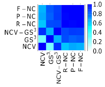
(a) (b)

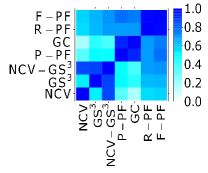
Figure 4: Pairwise relationships (Pearson correlations) between the six topological alignment quality measures over all alignments of (a) networks with known true node mapping and (b) networks with unknown true node mapping from four different species (i.e., yeast, fly, worm and human) containing four different types of PPIs (i.e., Y2H₁, Y2H₂, PHY₁, and PHY₂), for T. For T&S and S, see Supplementary Figures S1 and S5.

3.1.2 Comparison of LNA and GNA

To fairly evaluate LNA against GNA, we perform “all methods” and “best method” comparisons of the NA methods. By “all methods” comparison, we mean the following: to claim that LNA is better than GNA, each of the four LNA methods has to beat all four of the GNA methods. Analogously, to claim that GNA is better than LNA, each of the four GNA methods has to beat all four of the LNA methods. If none of the two conditions are met, then we say that neither LNA nor GNA is superior. By “best method” comparison, we mean the following: to claim that LNA is better than GNA, at least one LNA method has to beat all four of the GNA methods. Analogously, to claim that GNA is better than LNA, at least one GNA method has to beat all four of the LNA methods. If none of the two conditions are met, then we say that neither LNA nor GNA is superior. We perform each of the “all methods” and “best method” comparisons with respect to each of T, T&S, S, and B, where B is the best-case scenario, i.e., the best of T, T&S, and S. Namely, given two networks and a NA method, three alignments will be produced, one for each of T, T&S, and S. Then, B is the best of the three alignments with respect to the given alignment quality measure (different alignment quality measures might identify different alignments as B out of T, T&S, and S).

Overall, for both “all methods” and “best method” comparisons, we observe that GNA is superior to LNA in most of the cases for each of T, T&S, S, and B (Figure 5 and Supplementary Figure S2).

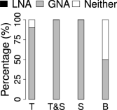
(a)           (b)

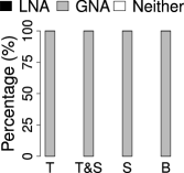
Figure 5: Overall comparison of LNA and GNA for networks with known true node mapping with respect to (a) “all methods” and (b) “best method” comparison, for T, T&S, S, and B. Each bar shows the percentage of the aligned network pairs (over both considered alignment quality measures combined) for which LNA is superior (black), GNA is superior (grey), or neither LNA nor GNA is superior (white). For detailed results, see Figure 6 and Supplementary Figures S3 and S4.

Next, we zoom into the results (Figure 6 and Supplementary Figures S3 and S4) to identify the best method(s). Recall that for LNA, NetworkBlast and NetAligner do not allow for using topological information in NCF. Thus, we cannot consider these methods for T and T&S. Given this, the results for LNA are as follows. For T and T&S, the remaining methods, AlignNemo and AlignMCL, are comparable (Figure 6 (a) and (b)). For S and B, of all four methods, AlignMCL is superior (Figure 6 (c) and (d)). Hence, we conclude AlignMCL to be the best LNA method. Recall that for GNA, NETAL does not allow for using sequence information in NCF. So, we cannot consider this method for T&S and S. (For this method, B is the same as T). Given this, the results for GNA are as follows. For all of T, T&S, S, and B, WAVE and MAGNA++ are the best methods. GHOST also performs well whenever sequence is used in NCF, i.e., for T&S, S, and B. However, for T, GHOST is inferior to all other methods. Hence, we conclude WAVE and MAGNA++ to be the best GNA methods. For both LNA and GNA, the choice of aligned networks impacts the results less for T&S and S than for T (as supported by smaller standard deviations in Figure 6 (b) and (c) compared to Figure 6 (a)).

(a) (b) (c) (d)

Figure 6: Detailed comparison of LNA and GNA for networks with known true node mapping with respect to F-NC and NCV-GS³ alignment quality measures, for (a) T, (b) T&S, (c) S, and (d) B. Each point represents alignment quality of the given NA method averaged over all network pairs, and each bar represents the corresponding standard deviation. A missing point indicates that the given NA method cannot use the corresponding type of information in NCF and thus no result is produced.

3.1.3 Summary

For networks with known true node mapping, GNA is superior to LNA. AlignMCL is superior of all LNA methods. WAVE and MAGNA++ are superior of all GNA methods.

3.2 Networks with unknown true node mapping

3.2.1 Relationships of different alignment quality measures

Similar to our analysis for networks with known true node mapping (Section 3.1.1), our first goal for four sets of networks with unknown true node mapping (Y2H₁, Y2H₂, PHY₁, and PHY₂, which encompass different species, PPI types, and PPI confidence levels; Section 2.1) is to understand potential redundancies of different alignment quality measures and choose the best and most representative of all redundant measures for fair evaluation of LNA and GNA. All reported results are for all four sets of networks combined, unless otherwise noted. In Section 3.2.3, we break down the results per network set, in order to evaluate their robustness to the choice of network data in terms of PPI type and confidence level.

For the networks with unknown node mapping, we use all seven measures: three topological (NCV, GS³, and NCV-GS³; Section 2.4.1) and four biological (P-PF, R-PF, F-PF, and GC; Section 2.4.2). For a given measure, we compute the score of aligning each of the 14 pairs of networks with known true node mapping (Section 2.1) with each of the eight NA methods (Section 2.2). Then, for each pair of measures, we compute the Pearson correlation coefficient across all of their $14\times 8=112$ alignment quality scores. We do this for each type of information used within NCF during alignment construction process, namely T, T&S, and S (Section 2.3).

Since the seven measures naturally cluster into two groups (one group consisting of the three topological measures that capture the size of the alignment in terms of the number of nodes or edges, and the other group consisting of the four biological measures that quantify the extent of functional similarity of the aligned nodes), we expect within-group correlations to be higher than across-group correlations. Indeed, this is what we observe overall for all of T, T&S, and S (Figure 4 (b) and Supplementary Figure S5; also, see Supplementary Section S6.2 for more details). Thus, since the two groups of measures evaluate alignment quality from different perspectives, since within each group the measures are redundant (Supplementary Section S6.2), and since in the first group NCV-GS³ combines NCV and GS³ (Section 2.4.1) while in the second group F-PF combines P-PF and R-PF (and is also redundant to the remaining GC measure), henceforth, we focus on NCV-GS³ as the most representative non-redundant topological measure and on F-PF as the most representative non-redundant biological measure.

3.2.2 Comparison of LNA and GNA

As in our analysis from Section 3.1.2, here we perform “all methods” and “best method” comparisons. For both comparison types, with respect to topological alignment quality, GNA is always superior to LNA for each of T, T&S, S, and B (Figure 7 (a), Supplementary Figure S6 (a), and Supplementary Figure S7). With respect to biological alignment quality, GNA is superior to LNA for T, while LNA is comparable or superior to GNA for T&S, S, and B (Figure 7 (b), Supplementary Figure S6 (b), and Supplementary Figure S7).

Next, we zoom into the above results (Figure 8 and Supplementary Figures S8-S12) in order to identify the best NA method(s). Recall that for LNA, NetworkBlast and NetAligner do not allow for using topological information in NCF. So, we cannot consider these methods for T and T&S. Given this, the results for LNA are as follows. With respect to topological alignment quality: for T and T&S, and B, AlignNemo is the best method; for S, AlignMCL is the best method. With respect to biological alignment quality: for T, AlignNemo is the best method; for T&S, AlignNemo and AlignMCL are the best methods and are comparable, with slight superiority of AlignNemo; for S and B, AlignMCL is the best method. Hence, we conclude AlignNemo and AlignMCL to be the best of all analyzed LNA methods, of which under the best-case scenario (B) AlignMCL is superior. Recall that for GNA, NETAL does not allow for using sequence information in NCF. So, we cannot consider this method for T&S and S. (Clearly, for this method, B is the same as T). Given this, the results for GNA are as follows. With respect to topological alignment quality: for T, NETAL is the best method; for T&S, WAVE is superior; for S, MAGNA++ is the best method; for B, NETAL is superior. With respect to biological alignment quality: for T, NETAL and GHOST are the best methods, with slight superiority of NETAL over GHOST; for T&S, GHOST is superior; for S and B, WAVE is the best method. Hence, we conclude that for GNA, in this analysis, the best method varies depending on whether we are measuring topological versus biological alignment quality and depending on the type of information used in NCF.

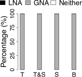
(a)      (b)

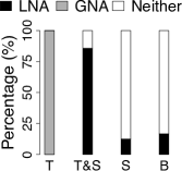
Figure 7: Overall comparison of LNA and GNA for networks with unknown true node mapping from four different species (i.e., yeast, fly, worm and human) containing four different types of PPIs (i.e., Y2H₁, Y2H₂, PHY₁, and PHY₂) with respect to (a) “all methods” comparison and the topological NCV-GS³ measure and (b) “all methods” comparison and the biological F-PF measure. Results are shown for T, T&S, S, and B. Each bar shows the percentage of the aligned network pairs for which LNA is superior (black), GNA is superior (grey), or neither LNA or GNA is superior (white). For “best methods” comparison results, see Supplementary Figure S6.

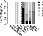
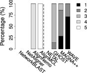
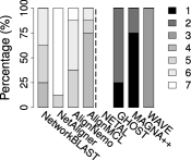
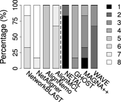
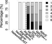
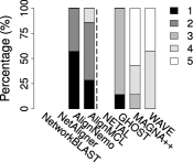
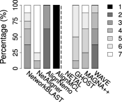
(a) (b) (c) (d) (e) (f) (g) (h)

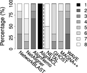
Figure 8: Detailed comparison of LNA and GNA for networks with unknown true node mapping from four different species (i.e., yeast, fly, worm and human) containing four different types of PPIs (i.e., Y2H₁, Y2H₂, PHY₁, and PHY₂) with respect to the topological NCV-GS³ measure (panels (a)-(d)) and the biological F-PF measure (panels (e) - (h)), for T (panels (a) and (e)), T&S (panels (b) and (f)), S (panels (c) and (g)), and B (panels (d) and (h)). Each bar shows the percentage of the aligned network pairs for which the given NA method performs as the $1^{st}$ best (1), $2^{nd}$ best (2), $3^{rd}$ best (3), etc. among all of the NA (LNA or GNA) methods with respect to the corresponding type of information used in NCF and the corresponding alignment quality measure. A missing bar indicates that the given NA method cannot use the corresponding type of information in NCF and thus no result is produced.

3.2.3 Robustness to the choice of network data

We aim to study the effect on results of using different network sets (PHY₁, PHY₂, Y2H₁, and Y2H₂), in order to test the robustness of the results to the choice of PPI type and confidence level. We find that for each of the “all methods” and “best method” comparisons, topological and biological alignment quality, and T, T&S, S and B, results are consistent across the different network sets (Supplementary Figure S13), and they are consistent with the above reported results for all four network sets combined (Figure 7). Thus, our NA evaluation framework is robust to the choice of network data.

3.2.4 Summary

Overall, when using only topological information in NCF, GNA outperforms LNA in terms of both topological and biological alignment quality. When adding sequence information to NCF, GNA is superior in terms of topological alignment quality, while LNA is superior in terms of biological quality. The best of all LNA methods are AlignMCL and AlignNemo. The best of all GNA methods varies depending on whether one is measuring topological versus biological alignment quality and on the type of information used in NCF. Importantly, our evaluation framework is robust to the choice of network data to be aligned.

The reason why GNA outperforms LNA in terms of topological alignment quality (meaning that GNA identifies larger amount of conserved edges and larger conserved subgraphs that LNA), irrespective of the type of NCF information used during the alignment construction process, could be due to the following key difference between the design goals of LNA and GNA. Namely, LNA aims to find small (on the order of a dozen nodes) but highly-conserved subnetworks, irrespective of the overall similarity between the compared networks. On the other hand, GNA aims to find a large conserved subgraph (though at the expense of matching local regions suboptimally), and typically it does so by directly optimizing edge conservation (and possibly other measures) while producing alignments. As such, simply by design, GNA might have an advantage over LNA in terms of the expected topological alignment quality, which our results confirm.

In terms of biological alignment quality, GNA again outperforms LNA for T. This indicates that when using within NCF only biological information encoded into network topology (i.e., when not using any biological information external to network topology, such as sequence information), GNA leads to better biological predictions than LNA. Also, in this case, the topological alignment quality results correlate well with the biological alignment quality results (as GNA is superior to LNA in both cases). However, when some amount of sequence information is included into NCF (corresponding to T&S and S), the topological alignment quality results do not correlate with the biological alignment quality results (as GNA is superior in the first case, while LNA is superior in the second case). The reason behind LNA’s superiority over GNA in terms of biological alignment quality for T&S and S could again be due to differences in their key design goals. Namely, unlike GNA, LNA uses the notion of the alignment graph to search for highly conserved subnetworks (Supplementary Section S2). When sequence information is used within NCF, nodes in this graph contain sequence-based orthologs, i.e., highly sequence-similar proteins from different networks. Since high sequence similarity often corresponds to high functional similarity, and since our measures of biological alignment quality are based on the notion of functional similarity between aligned proteins, by design LNA is “biased” towards resulting in high biological quality whenever sequence information is used in NCF. However, LNA fails to produce biologically as good alignments as GNA when only topological information is used in NCF, as discussed above.

3.3 Running time method comparison

The results from Sections 3.1 and 3.2 compare the different methods in terms of alignment accuracy. It is also important to compare the methods in terms of computational complexity, which is the goal of this section.

We run all NA methods on the same Linux machine with 64 CPU cores (AMD Opteron(tm) Processor 6378) and 512 GB of RAM. Since some NA methods (all LNA methods, as well as NETAL and WAVE GNA methods) can only run on one core while the others (GHOST and MAGNA++ GNA methods) can run on multiple cores, for fair comparison, we run all methods on a single CPU core. An exception is GHOST, as its implementation still uses two threads even when its code is configured to use one core. We analyze the methods’ entire running times, both for computing node similarities and for constructing alignments. Also, we measure only running times needed to construct alignments, ignoring the time needed to precompute node similarities. We do the above when aligning worm and yeast PPI networks of Y2H₁ type (Table 1). We choose these networks because both are relatively small, and thus, the execution time for the slowest of all methods on a single core is reasonable (within one day). For any other network pair, running the slowest method on a single core would take much longer.

Our findings are as follows. For the entire running time, overall, for T, GNA is faster than LNA; for T&S, GNA methods run similarly to LNA methods. For S, LNA is faster than GNA. For only the time needed to construct alignments, overall, LNA methods run faster than GNA methods for each of T, T&S, and S (Table 1 and Supplementary Section S6.3).

In addition to the above single-core analysis, we give each method the best-case advantage, by running the parallelizable methods (GHOST and MAGNA++ GNA methods) on multiple cores; we use as many cores as possible with the given method implementation, where 64 cores is the maximum imposed by our machine. We show these results also in Table 1, in parentheses. As expected, running the two NA methods on multiple cores indeed speeds up the methods’ running times. We do not necessarily see a linear decrease in running time with the increase in the number of cores, as not all parts of the given method are parallelizable.

Our results for the best-case, multi-core analysis are as follows. For the entire running time, for T, GNA remains faster than LNA. However, for T&S and S, unlike in the above single-core analysis where LNA is comparable or superior to GNA, GNA is now always comparable (if not even superior) to LNA. For only the time needed to construct alignments, LNA mostly remains faster than GNA (Table 1 and Supplementary Section S6.3).

Type	Method	Entire time (min)			Only time needed to
					construct alignments (min)
		T	T&S	S	T	T&S	S
LNA	NetworkBLAST	-	-	372.6	-	-	7.3
	NetAligner	-	-	368.2	-	-	2.35
	AlignNemo	375.5	450.3	370.0	4.9	0.4	0.4
	AlignMCL	377.0	452.1	365.2	1.6	1.75	1.7
GNA	NETAL	0.4	-	-	0.4	-	-
	GHOST	78.2	438.5	435.3	7.5	9.5	10.7
		(16.8)	(381.8)	(378.1)	(4.2)	(6.5)	(6.4)
	MAGNA++	287.8	768.9	690.7	224.6	225.2	221.7
		(31.6)	(474.4)	(383.4)	(14.7)	(14.3)	(14.1)
	WAVE	17.15	450.8	369.7	2.9	3.1	2.8

Table 1: Representative running time comparison of the different NA methods, for each of T, T&S, and S. Both the entire running times and only the running times for computing alignments are shown. Values outside parentheses are for the single-core analysis, while values in parentheses are for the multi-core analysis (when applicable). The ‘-’ character indicates that the given method cannot use the corresponding type of information in NCF and thus no result is produced.

3.4 Novel protein function predictions

Finally, we contrast LNA against GNA in the context of learning novel protein functional knowledge. We identify alignments in which the aligned network regions are significantly functionally similar according to known functional knowledge. Then, from such alignments, we predict novel functional knowledge in currently unannotated network regions whenever such regions are aligned to functionally annotated network regions (Section 2.5).

We find that LNA and GNA produce very different predictions, indicating their complementarity when learning new knowledge. Of the predictions made by all (LNA or GNA) methods for all of T, T&S, and S, significant portion come from LNA only or GNA only, and only 9.1% come from both LNA and GNA (Figure 9 (a)).

We zoom into the above results for each of LNA (Supplementary Figure S14) and GNA (Figure 9 (b)) to study the effect on the prediction results of using different types of information in NCF. We aim to test whether using some amount of topological information in NCF (corresponding to T or T&S) can yield unique predictions that are not captured when using only sequence information in NCF (corresponding to S). If so, this would confirm that additional biological knowledge is encoded in network topology compared to sequence data. Indeed, this is what we observe, for each of LNA and GNA: most predictions are unique to the different types of NCF information. Thus, network topology and sequence information complement each other when learning new biological knowledge.

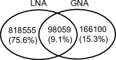
(a) (b)

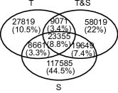
Figure 9: Overlap of unique novel protein function predictions between (a) LNA and GNA over all of T, T&S, and S combined, (b) T, T&S, and S for GNA. See Supplementary Figure S14 for overlap of unique novel protein function predictions between T, T&S, and S for LNA.

4 Conclusions

In this paper, we systematically evaluate LNA against GNA. Our findings provide guidelines for researchers to properly demonstrate the superiority of a newly proposed NA (LNA or GNA) method. That is, we recommend that researchers evaluate the topological quality of a new NA method against state-of-the-art GNA (rather than only LNA) methods, irrespective of the type of information used in NCF, and that they evaluate the biological alignment quality of the new NA method against state-of-the-art GNA (rather than only LNA) methods when only T is used in NCF and against LNA (rather than only GNA) methods when S is also used in NCF. NA can be used to complement the across-species transfer of functional knowledge that has traditionally relied on sequence alignment.

References

- [1] B. J. Breitkreutz et al. The BioGRID Interaction Database: 2008 update. Nucleic Acids Research, 36:D637–D640, 2008.
- [2] K R Brown and I Jurisica. Unequal evolutionary conservation of human protein interactions in interologous networks. Genome Biology, 8(5):R95, 2007.
- [3] Giovanni Ciriello et al. AlignNemo: a local network alignment method to integrate homology and topology. PLOS ONE, 7(6):e38107, 2012.
- [4] S.R. Collins et al. Toward a comprehensive atlas of the physical interactome of saccharomyces cerevisiae. Molecular Cell Proteomics, 6(3):439–450, 2007.
- [5] Joseph Crawford, Yihan Sun, and Tijana Milenković. Fair evaluation of global network aligners. Algorithms for Molecular Biology, 10(1):1–17, 2015.
- [6] Michael E Cusick et al. Literature-curated protein interaction datasets. Nature Methods, 6(1):39–46, 2009.
- [7] F. Faisal, L. Meng, J. Crawford, and T. Milenković. The post-genomic era of biological network alignment. EURASIP Journal on Bioinformatics and Systems Biology, 2015(1):1–19, 2015.
- [8] F.E. Faisal, H. Zhao, and T. Milenković. Global network alignment in the context of aging. IEEE/ACM Transactions on Computational Biology and Bioinformatics, 12(1):40–52, Jan 2015.
- [9] Matthias Gstaiger and Ruedi Aebersold. Applying mass spectrometry-based proteomics to genetics, genomics and network biology. Nature Reviews Genetics, 10:617–627, 2009.
- [10] Somaye Hashemifar and Jinbo Xu. HubAlign: an accurate and efficient method for global alignment of protein–protein interaction networks. Bioinformatics, 30(17):i438–i444, 2014.
- [11] Jialu Hu and Knut Reinert. LocalAli: an evolutionary-based local alignment approach to identify functionally conserved modules in multiple networks. Bioinformatics, 31(3):363–372, 2015.
- [12] Rashid Ibragimov, Maximilian Malek, Jiong Guo, and Jan Baumbach. GEDEVO: An evolutionary graph edit distance algorithm for biological network alignment. German Conference on Bioinformatics (GCB), 34:68–79, 2013.
- [13] M. Kanehisa et al. Data, information, knowledge and principle: back to metabolism in KEGG. Nucleic Acids Research, 42:D199 –D205, 2014.
- [14] O. Kuchaiev, T. Milenković, V. Memišević, W. Hayes, and N. Pržulj. Topological network alignment uncovers biological function and phylogeny. Journal of the Royal Society Interface, 7:1341–1354, 2010.
- [15] O. Kuchaiev and N. Pržulj. Integrative network alignment reveals large regions of global network similarity in yeast and human. Bioinformatics, 27(10):1390–1396, 2011.
- [16] Noël Malod-Dognin and Nataša Pržulj. L-GRAAL: Lagrangian graphlet-based network aligner. Bioinformatics, 31:2182–2189, 2015.
- [17] Vesna Memišević and Nataša Pržulj. C-GRAAL: Common-neighbors-based global graph alignment of biological networks. Integrative Biology, 4(7):734–743, 2012.
- [18] T. Milenković, W.L. Ng, W. Hayes, and N. Pržulj. Optimal network alignment with graphlet degree vectors. Cancer Informatics, 9:121–137, 2010.
- [19] Marco Mina and Pietro Hiram Guzzi. AlignMCL: Comparative analysis of protein interaction networks through markov clustering. In Proceedings of the 2012 IEEE International Conference on Bioinformatics and Biomedicine Workshops (BIBMW), pages 174–181, 2012.
- [20] Behnam Neyshabur, Ahmadreza Khadem, Somaye Hashemifar, and Seyed Shahriar Arab. NETAL: a new graph-based method for global alignment of protein-protein interaction networks. Bioinformatics, 29(13):1654–1662, 2013.
- [21] Roland A Pache and Patrick Aloy. A novel framework for the comparative analysis of biological networks. PLOS ONE, 7(2):e31220, 2012.
- [22] R Patro and C Kingsford. Global network alignment using multiscale spectral signatures. Bioinformatics, 28(23):3105–3114, 2012.
- [23] V. Saraph and T. Milenković. MAGNA: Maximizing Accuracy in Global Network Alignment. Bioinformatics, 30(20):2931–2940, 2014.
- [24] Boon-Siew Seah, Sourav S Bhowmick, and C Forbes Dewey. DualAligner: a dual alignment-based strategy to align protein interaction networks. Bioinformatics, 30:2619–2626, 2014.
- [25] R. Sharan et al. Conserved patterns of protein interaction in multiple species. Proceedings of the National Academy of Sciences of the United States of America, 102(6):1974–1979, 2005.
- [26] R. Singh, J. Xu, and B. Berger. Pairwise global alignment of protein interaction networks by matching neighborhood topology. In Research in Computational Molecular Biology, pages 16–31, 2007.
- [27] Yihan Sun, Joseph Crawford, Jie Tang, and Tijana Milenković. Simultaneous optimization of both node and edge conservation in network alignment via WAVE. In Workshop on Algorithms in Bioinformatics (WABI), pages 16–39, 2015.
- [28] Andrei Todor, Alin Dobra, and Tamer Kahveci. Probabilistic biological network alignment. IEEE/ACM Transactions on Computational Biology and Bioinformatics, 10(1):109–121, January 2013.
- [29] V Vijayan, V Saraph, and T Milenković. MAGNA++: Maximizing accuracy in global network alignment via both node and edge conservation. Bioinformatics, 31(14):2409–2411, 2015.
- [30] H. Yu et al. High-quality binary protein interaction map of the yeast interactome networks. Science, 322:104–110, 2008.