A circumbinary disc model for the variability of the eclipsing binary CoRoT 223992193

Abstract

We calculate the flux received from a binary system obscured by a circumbinary disc. The disc is modelled using two dimensional hydrodynamical simulations, and the vertical structure is derived by assuming it is isothermal. The gravitational torque from the binary creates a cavity in the disc’s inner parts. If the line of sight along which the system is observed has a high inclination $I$, it intersects the disc and some absorption is produced. As the system is not axisymmetric, the resulting light curve displays variability. We calculate the absorption and produce light curves for different values of the dust disc aspect ratio $H/r$ and mass of dust in the cavity $M_{\rm dust}$. This model is applied to the high inclination ($I=85\degr$) eclipsing binary CoRoT 223992193, which shows 5–10% residual photometric variability after the eclipses and a spot model are subtracted. We find that such variations for $I\sim 85\degr$ can be obtained for $H/r=10^{-3}$ and $M_{\rm dust}\geq 10^{-12}$ M_☉. For higher $H/r$, $M_{\rm dust}$ would have to be close to this lower value and $I$ somewhat less than $85\degr$. Our results show that such variability in a system where the stars are at least 90% visible at all phases can be obtained only if absorption is produced by dust located inside the cavity. If absorption is dominated by the parts of the disc located close to or beyond the edge of the cavity, the stars are significantly obscured.

1 Introduction

In the course of CSI 2264, an international photometric monitoring campaign of several hundred young stars located in the NGC2264 star forming region (Cody et al. 2014), Gillen et al. (2014) reported the discovery of CoRoT 223992193, a double–lined eclipsing binary consisting of two M–type pre–main sequence (PMS) stars. The analysis of the CoRoT 223992193 light curves completed by radial velocity measurements yielded a complete characterisation of the orbit of the tight system (P=3.8745745 days) as well as a precise determination of the mass and radius of each component. At an age of 3.5–6 Myr, this eclipsing system provides strong constraints on the validity of low–mass PMS evolutionary models (Gillen et al. 2014, Stassun et al. 2014).

Interestingly, the CoRoT 223992193 light curve also reveals significant variability outside of the eclipses. Part of the large amplitude (10–15%) and rapidly evolving out–of–eclipse variations can be accounted for by surface spots, but there is a residual variability with an amplitude of 5–10% (Gillen et al. 2015). Based on the high system’s inclination ($I$=85$\degr$) and the presence of significant near/mid–infrared excess, it was suggested that at least part of the observed variability could be due to hot dust orbiting the inner system and, as it rotates, partially occults the central stellar components (Gillen et al. 2014, 2015).

Here, we investigate this possibility further by running numerical simulations of a binary system, whose properties are those of CoRoT 223992193, and which is surrounded by a circumbinary dusty disc. Similar models of discs around binaries have been published previously (e.g., Hanawa et al. 2010, de Val–Borro et al.  2011, Shi et al. 2012, Shi & Krolik 2015), but our numerical modelling specifically aims to reproduce the out–of–eclipse variability of CoRoT 223992193. Assuming that the system is seen along a line of sight with a given inclination angle $I$, we calculate the mass of dust that the line of sight intersects from the disc, and the resulting light curve.

The plan of the paper is as follows. In section 2, we present two dimensional numerical simulations of the circumbinary disc around a binary system like CoRoT 223992193. In section 3, we explain how the light curves are calculated and derive the parameters that give the best fit to the CoRoT 223992193 system. Finally, in section 4, we summarise and discuss our results.

2 Numerical simulations of circumbinary discs

We consider a binary system and a circumbinary disc which lies in the orbital plane. The angular velocity of the binary is $\Omega_{\rm bin}=\sqrt{G(M_{1}+M_{2})/a^{3}}$, where $G$ is the gravitational constant, $M_{1}$ and $M_{2}$ are the masses of the stars and $a$ is the separation. The binary is assumed to have a circular orbit. In the frame corotating with the binary and with origin at the centre of mass, in two dimensions, the equation of motion for a fluid element in the disc with position vector ${\bf r}$ and velocity ${\bf v}$ is:

$$\frac{\partial{\bf v}}{\partial t}+\left({\bf v}\cdot\mbox{\boldmath$\nabla$}\right){\bf v}=-\frac{1}{\Sigma}\mbox{\boldmath$\nabla$}P-\mbox{\boldmath$\nabla$}\Phi-\mbox{\boldmath$\Omega$}_{\rm bin}\mbox{\boldmath$\times$}\left(\mbox{\boldmath$\Omega$}_{\rm bin}\mbox{\boldmath$\times$}{\bf r}\right)-2\mbox{\boldmath$\Omega$}_{\rm bin}\mbox{\boldmath$\times$}{\bf v},$$ (1)

where $P$ is the pressure averaged over the disc scale height, $\Sigma$ is the surface mass density, $\mbox{\boldmath$\Omega$}_{\rm bin}=\Omega_{\rm bin}\hat{\bf z}$, with $\hat{\bf z}$ being the unit vector perpendicular to the disc plane, and $\Phi$ is the gravitational potential due to the stars. We assume that the disc’s mass is small compared to that of the stars, so that self–gravity can be neglected. We have:

$$\Phi=-\frac{GM_{1}}{\left|{\bf r}-{\bf r}_{1}\right|}-\frac{GM_{2}}{\left|{\bf r}-{\bf r}_{2}\right|},$$ (2)

where ${\bf r}_{1}$ and ${\bf r}_{2}$ are the position vectors of the stars with masses $M_{1}$ and $M_{2}$, respectively.

The surface mass density also has to satisfy the mass conservation equation:

$$\frac{\partial{\Sigma}}{\partial t}+\mbox{\boldmath$\nabla$}\cdot\left(\Sigma{\bf v}\right)=0.$$ (3)

Finally, we adopt an isothermal equation of state for the gas:

$$P=\Sigma c_{s}^{2},$$ (4)

where $c_{s}$ is the isothermal sound speed.

2.1 Initial conditions

In the corotating frame with origin at the centre of mass, we note $(x,y,z)$ the cartesian coordinates, where $x$ is the axis passing through the centres of the stars and $z$ is perpendicular to the orbital plane, and $(r,\theta,z)$ the associated polar coordinates. The coordinate of the primary star, of mass $M_{1}$, is $x_{1}=-aM_{2}/(M_{1}+M_{2})$, whereas the coordinate of the secondary star, of mass $M_{2}$, is $x_{2}=aM_{1}/(M_{1}+M_{2})$. Initially, the disc extends from an inner radius $R_{\rm in}$ to some outer radius.

Following Hanawa et al. (2010), we take the initial density profile to be:

$$\Sigma_{\rm init}=\Sigma_{0}\left(0.55+0.45\tanh\frac{r-\mbox{$R_{\rm in}$}}{h}\right)+\Sigma_{\rm min}.$$ (5)

The constant $\Sigma_{0}$ is related to the total mass of the disc and $\Sigma_{\rm min}$, which we choose to be very small compared to $\Sigma_{0}$, is added to ensure that the mass density does not become smaller than some threshold to avoid numerical problems. The above equation is such that $\Sigma_{\rm init}\simeq 0$ at the disc’s inner edge, increases to $\Sigma_{0}$ over a scale $h$ and is uniform equal to $\Sigma_{0}$ beyond.

As the binary perturbs significantly the disc only over a very limited region near its inner edge, over which the surface density is not expected to vary much, we will only consider models with an initial uniform surface density, as given by equation (5).

The initial velocity in the disc is set to be the Keplerian velocity in the rotating frame:

$${\bf v}_{\rm init}=r\left(\Omega_{\rm K}-\Omega_{\rm bin}\right)\hat{\mbox{\boldmath$\theta$}},$$ (6)

with $\Omega_{\rm K}=\sqrt{G(M_{1}+M_{2})/r^{3}}$ and $\hat{\mbox{\boldmath$\theta$}}$ is the unit vector in the azimuthal direction.

2.2 Units

In the numerical simulations, we take $G=1$, $a=1$, $M_{1}=0.7$ and $M_{2}=0.5$. Therefore, all the lengths will be given in units of the binary separation. In this unit system, the timescale $\Omega_{\rm bin}^{-1}$ is approximately $0.91$ and the orbital period is $2\pi/\Omega_{\rm bin}\simeq 5.74$.

With the equation of state (4), the pressure term in equation (1) does not depend on $\Sigma_{0}$. Since, in addition, the disc is non self–gravitating, its mass does not enter the equations. Therefore we can take $\Sigma_{0}=1$.

2.3 Numerical set up and boundary conditions

Equations (1), (3) and (4) are solved with the initial conditions (5) and (6) using version 4.0 of the PLUTO code (Mignone et al. 2007). No explicit viscosity is used.

Although a polar coordinate system would be a natural choice to describe the evolution of the disc, it would involve a singularity at the origin and therefore would not be numerically tractable. Therefore, we set up a cartesian grid. We use three consecutive adjacent grids in the $x$ and $y$ directions. They extend from $-15$ to $-2$, $-2$ to $2$ and $2$ to $15$ and each has 1024 zones in both directions. The outer radius of the disc does not need to be specified as long as it is beyond the edge of the grid.

To prevent the gravitational potential from becoming infinite when a particle approaches one of the stars very closely, we soften it by replacing $\left|{\bf r}-{\bf r}_{1,2}\right|$ by ${\rm max}\left(\left|{\bf r}-{\bf r}_{1,2}\right|,d_{\rm soft}\right)$ in equation (2), where $d_{\rm soft}$ is the softening parameter. We take $d_{\rm soft}=0.07$.

When the surface density becomes very small, the code does not perform very well. Therefore, we fix a threshold $\Sigma_{\rm min}=10^{-3}$ and replace the density by this value wherever it becomes smaller. Following Hanawa et al. (2010), we also fix $h=0.144$ in equation (5).

To prevent wave reflection at the outer edge of the grid, we use the wave killing condition described in de Val–Borro et al. (2006). This procedure forces the variables to relax toward their initial values on some prescribed timescale in a region close to the outer edge of the grid.

The wave killing procedure is used when waves would otherwise be reflected at the grid outer boundary. Therefore, this boundary stays close to its initial state and has little effect on the dynamics of the flow in the disc’s inner parts. Therefore, our boundary conditions are:

$$F=F_{\rm init},$$ (7)

at the edge of the grid, where $F$ is either $\rho$, $P$, $v_{x}$ or $v_{y}$.

2.4 Results

Figure 1 shows the surface density $\Sigma$ in the $x$–$y$ plane in a disc that has reached a steady–state for a sound speed $c_{s}=0.3$.

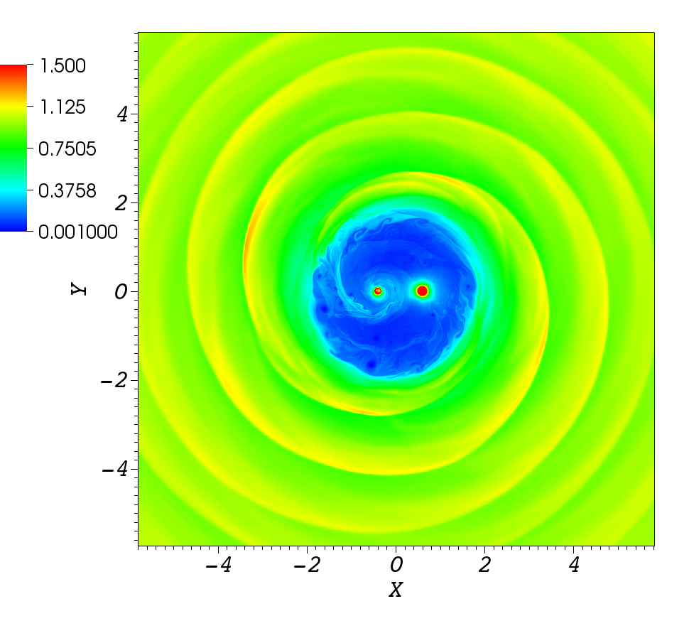
Figure 1: Pseudocolor plot of the surface density $\Sigma$ in the $x$–$y$ plane for a sound speed $c_{s}=0.3$. The primary and secondary stars are located at $(-0.42,0)$ and $(0.58,0)$, respectively. The mapping of data to color values is linear.

The circumbinary disc is set up with an inner edge at $\mbox{$R_{\rm in}$}=2.5$. As can be seen from figure 1, the material near this edge is pushed inward by pressure forces. The gravitational torque exerted by the binary opposes pressure forces, so that a cavity with a radius of about 2 is created. This is consistent with theory, which predicts a disc’s inner radius of roughly twice the binary separation (Lin & Papaloizou 1979). Some mass though does penetrate inside the cavity, as seen in previous simulations.

The maximum value of $\Sigma$ along the density waves launched at the inner edge of the disc is about 1.5. Circumstellar discs form around the stars. Their radius is about 0.3–0.4 for the primary star and 0.2–0.3 for the secondary star (as seen in figure 1, the disc around the secondary is denser but actually not as extended). Again, this is consistent with theory, as tidal truncation of the circumstellar discs by the other star is expected to limit their outer radii to about one third of the binary separation (Paczynski 1977, Papaloizou & Pringle 1977). In the inner parts of these circumstellar discs, $\Sigma$ becomes large as material piles up. In figure 1, $\Sigma$ in the inner parts of the circumstellar discs is saturated. In reality though, mass from these discs would be accreted onto the stars and/or launched into jets. As we will see below, since dust in the inner parts of the circumstellar discs is sublimated by stellar radiation, the detailed structure of these discs does not affect the results presented in this paper.

As this map of the surface density around a binary system is very typical, and is similar to that obtained in many previous studies (see, e.g., Hanawa et al. 2010, Shi & Krolik 2015), we will focus on this single particular case in this paper. We have run models with different sound speeds but they all give similar results.

3 Binary light curve

3.1 Disc vertical structure

The numerical simulations we have performed are two dimensional, and therefore we only calculate the surface mass density:

$$\Sigma(x,y)=\int_{-\infty}^{\infty}\rho(x,y,z)dz,$$ (8)

where $\rho$ is the density per unit volume. To generate the third dimension, we assume that the disc is isothermal in the vertical direction with a scale–height $H$, so that:

$$\rho(x,y,z)=\rho_{0}(x,y)\;{\rm e}^{-z^{2}/(2H^{2})},$$ (9)

where $\rho_{0}$ is the density in the disc midplane (at $z=0$). Then equation (8) yields:

$$\Sigma(x,y)=\sqrt{2\pi}\rho_{0}(x,y)H(x,y),$$ (10)

where $H$ may depend on $x$ and $y$. Then equation (9) becomes:

$$\rho(x,y,z)=\frac{\overline{\rho}\Sigma(x,y)}{\sqrt{2\pi}H}\;{\rm e}^{-z^{2}/(2H^{2})},$$ (11)

where $\overline{\rho}$ is a constant factor by which we scale the density obtained in the simulations (it can be chosen by requiring a given total mass for the disc). Equation (11) is used to construct $\rho$ from $\Sigma$.

The simulations presented in section 2 were done for a constant sound speed $c_{s}=0.3$ in code units. When hydrostatic equilibrium is reached in the vertical direction, this corresponds to a gas disc scale height $H=c_{s}/\Omega_{\rm K}=0.27r^{3/2}$. For the calculation to be self–consistent, this is the value that should be used when calculating the binary light curve. However, the gas is completely transparent to stellar radiation, and absorption is due solely to dust grains which are mixed with the gas. The dust disc scale height might differ significantly from the gas scale height if, for example, dust grains are not well mixed all the way up with the gas. Therefore, in the following section, we will allow $H$ to depart from the value given above. For simplicity, we will consider $H/r={\rm const}$, and will vary this value until we obtain a light curve which matches that of the system which is being modelled. The implications of the value of $H/r$ found below will be discussed in section 4.

3.2 Light curve modelling

To obtain the light curve of the system, we calculate, for each star, the amount of energy that comes out of a cylinder whose base is the projected surface of the star and whose axis is the line of sight (see figure 2). Part of the flux emitted by the stars is absorbed by the disc if the cylinders intersect it. Each cylinder is split into multiple line of sights in the z–direction and sliced up into a number of bins $j=1,\dotsc,n$ along each line of sight. The total mass $m_{j}$ in each bin is the mass in the part of the disc which is intersected by the bin. To obtain this mass, we integrate each density datapoint over its volume element, assign a weight to the volume elements in the disc depending on how far they are from the axis of the cylinder, and sum up over all these points. We calculate a mean density $\rho_{j}$ in the bin by dividing the mass $m_{j}$ by the volume of the bin. The intensity transferred from the bin $j$ to the bin $j+1$ (going away from the star) is therefore $I_{j+1}=I_{j}{\rm e}^{-\tau_{j}}$, where $\tau_{j}=\kappa\rho_{j}\Delta l_{j}$ is the optical depth, with $\kappa$ being the opacity and $\Delta l_{j}$ being the length of the bin along the axis of the cylinder. In the calculations presented below, we will take $\kappa=5$ cm² g^-1 (Jensen & Mathieu 1997). This assumes that gas and dust are well mixed and that the gas to dust ratio is 100.

In this paper, we calculate the light curve of a system which has the characteristics of CoRoT 223992193 (Gillen et al. 2014). The primary star has a mass $M_{1}=0.7$ M_⊙ and a radius $R_{1}=1.3$ R_⊙, the secondary has a mass $M_{2}=0.5$ M_⊙ and a radius $R_{2}=1.1$ R_⊙ and their separation is $a=0.05$ au. So the unit of distance $a$ that we have used in the previous section corresponds to a physical distance of 0.05 au. Using the effective temperatures $T_{1}=3700$ K and $T_{2}=3600$ K estimated by Gillen et al. (2014), we infer the luminosities $L_{1}=0.28$ L_⊙ and $L_{2}=0.18$ L_⊙ (which corresponds to $L_{2}/L_{1}=0.64$, as observed).

The sublimation radii are 3.9 and 3.2 solar radii for the primary and secondary stars, respectively (Gillen et al. 2014). It means that no obscuration of the stars can come from material within a distance of 0.37 and 0.30 from the primary and secondary stars, respectively. To calculate the emergent stellar intensities, we therefore exclude the parts of the disc within $\mbox{$r_{\rm min}$}={\rm max}\left(0.42+0.37,0.58+0.30\right)\simeq 0.9=0.045$ au (the primary and secondary stars are located at $x=-0.42$ and $x=0.58$, respectively).

In the simulations presented in the previous section, the disc is only modelled up to some outer radius given by the boundary of the grid. For the range of line of sight inclinations we consider, we find that absorption of the stellar fluxes is due to the parts of the disc which are much smaller than this outer radius. Therefore the finite size of the grid is not a limitation of the model.

Figure 2 gives a schematic view of the system. In this sketch, the disc has been represented as though it had a finite thickness, but there is actually mass at all altitudes above the midplane as the density varies according to equation (9). Therefore, there is always some mass in every bin along the cylinders, even if only a tiny amount.

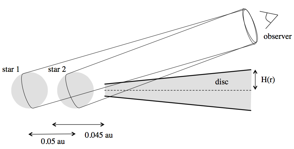
Figure 2: Schematic view of the system for which we calculate light curves.

We define the viewing angle $\theta$ as the angle between the projection of the line of sight in the $(x,y)$ plane and the $x$–axis. A viewing angle $\theta=0$ means that the observer looks at the system along the line joining the centres of the stars and with the secondary being in front (primary eclipse), i.e. from the right on figures 1 and 2. This angle increases when the line of sight rotates clockwise for a fixed binary, as in figure 1, which is equivalent to rotating the binary anti–clockwise for a fixed line of sight (as in the realistic situation). We also define the inclination angle $I$ between the line of sight and the perpendicular to the orbital plane ($I=0$ means that the system is seen pole–on).

The light curve is the amount of flux received from the system as a function of time for a fixed line of sight. If the disc is in quasi–steady state, as is the case here, rotating the disc for a fixed line of sight is equivalent to varying the viewing angle $\theta$. Therefore, the light curve of the system is obtained by calculating the flux as a function of $\theta$.

3.3 Results

As mentioned in the introduction, the light curve of CoRoT 223992193 displays out–of–eclipse variations which have a peak–to–peak amplitude of about 15% (Gillen et al 2014). Part of this variability can be explained by a spot model, but the residuals show extra variability with an amplitude of about 5-10% (Gillen et al. 2015). The system is seen with $I=85\degr$ and the visual extinction is estimated to be between 0 and 0.1 (Gillen et al. 2014), which means that there could be an extinction of the stars of up to 10% at all orbital phases.

Here, we investigate whether the residual variability can be explained by obscuration of the stars by the circumbinary and/or circumstellar discs.

We calculate the light curve of the system in the way described in the previous section, and vary $H/r$ and $\overline{\rho}$ (see eq. [11]) until we obtain a curve which displays 5–10% variations for values of $I$ close to 85$\degr$. We define the disc’s inner cavity as the region between $r=\mbox{$r_{\rm min}$}=0.9$ and $r=2$. We present results for $H/r=10^{-3}$ and 0.05, and for values of $\overline{\rho}$ corresponding to a mass of dust in the disc’s inner cavity $M_{\rm dust}=10^{-12}$ and $10^{-11}$ M_☉.

The largest value of $H/r$ we consider would be expected in a disc in which the sound speed is about 10% of the Keplerian velocity and the dust is well mixed with the gas all the way through the disc’s thickness, whereas the smallest value would be typical of a disc with very small pressure forces and/or dust not well mixed with the gas. Note that in this calculation we assume that the mass of dust is about one hundredth of the mass of gas, and the two components are well mixed. This assumption will be discussed in section 4.

The flux versus viewing angle is displayed in figure 3 for $H/r=10^{-3}$ and $M_{\rm dust}=10^{-12}$ and $10^{-11}$ M_☉, and in figure 4 for $H/r=0.05$ and the same values of $M_{\rm dust}$. Note that the flux has been divided by the value it would have if the stars were unobscured (i.e. if there were no disc).

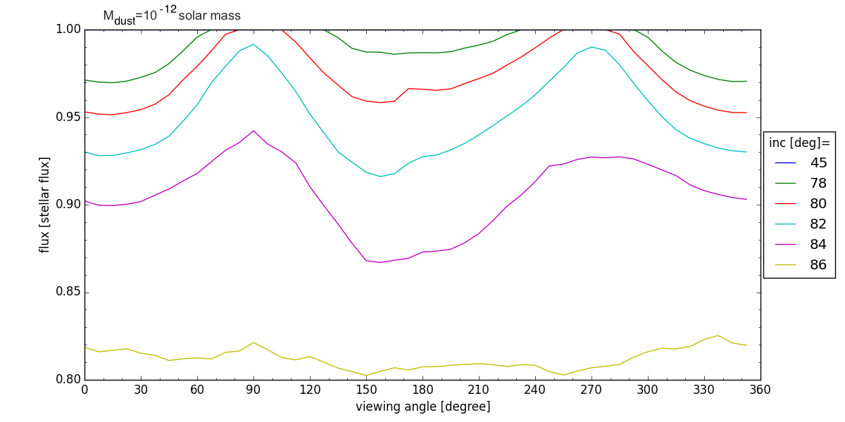
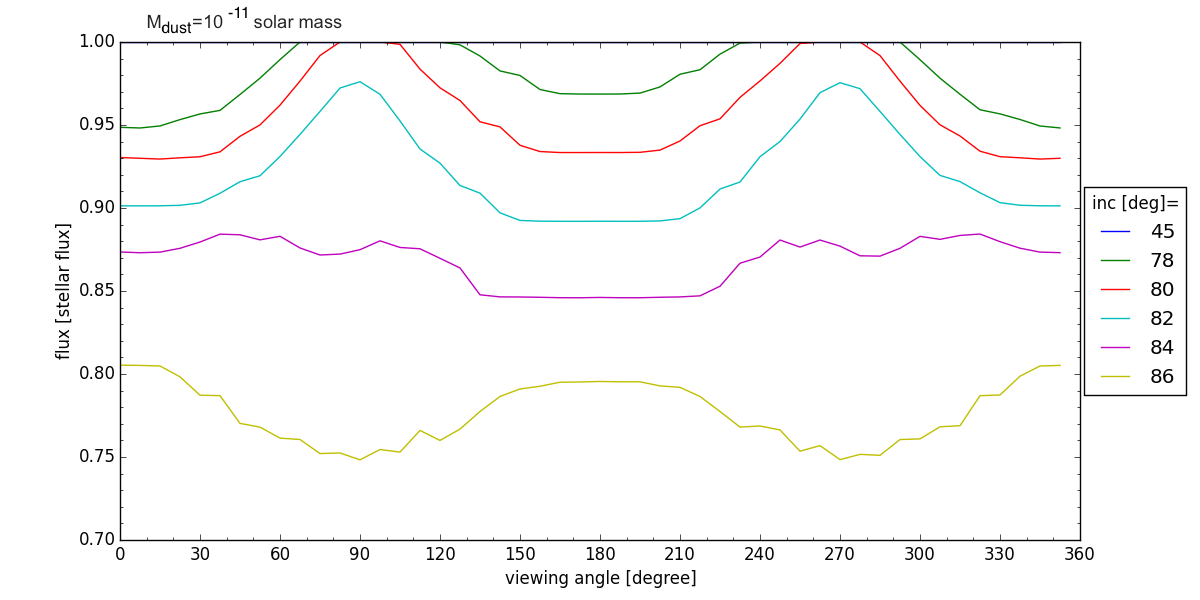
Figure 3: Flux divided by the unobscured value versus viewing angle (in degrees) for $H/r=10^{-3}$. The upper and lower plots correspond to $M_{\rm dust}=10^{-12}$ and $10^{-11}$ M_☉, respectively. The curves have been calculated for different inclination angles $I=45$, 78, 80, 82, 84 and 86$\degr$. The curve corresponding to $I=45\degr$ is flat and corresponds to a flux equal to 1. The curves which ressemble most that of CoRoT 223992193 are the one corresponding to $I=78$–$82\degr$. In the case of $M_{\rm dust}=10^{-12}$ M_☉, $I=84\degr$ would also give a good fit.

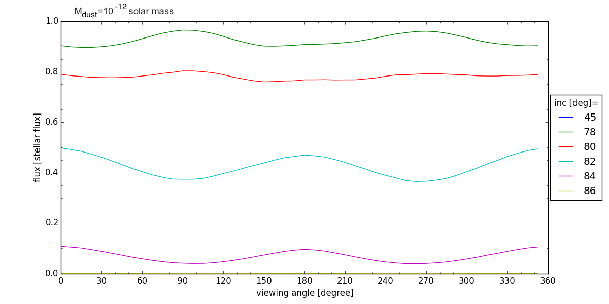
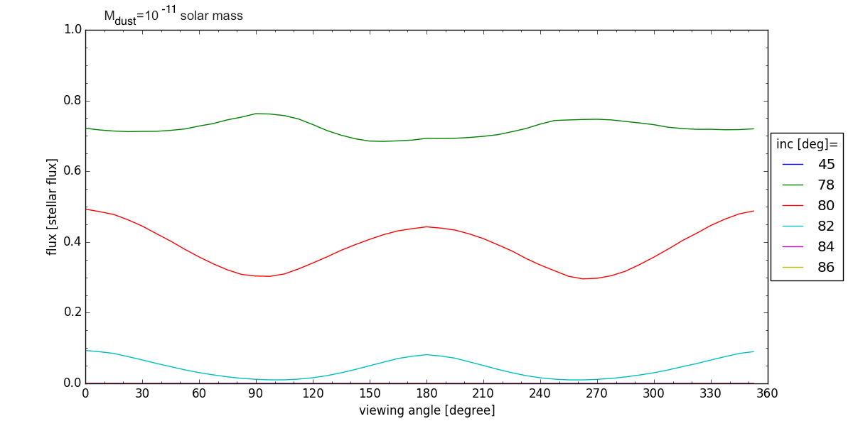
Figure 4: Same as figure 3 but for $H/r=0.05$. Here, only $I=78\degr$ for $M_{\rm dust}=10^{-12}$ M_☉ would match the CoRoT 223992193 light curve.

The eclipses of the stars by each other have not been taken into account in the calculation of the light curves, i.e. the emergent stellar fluxes have been calculated separately for the two cylinders represented in figure 2 and then added. The curves therefore show the out–of–eclipse variations. The eclipses would produce additional narrow “dips” in the light curves at $\theta=0$ and 180$\degr$.

When $\theta=0$, the cylinder based on the secondary star intersects a larger portion of the disc than the cylinder based on the primary star (see figure 2). Therefore, the secondary star is at least partially hidden for the inclinations $I$ we have considered (except 45$\degr$), while the primary may still be fully visible. If the secondary star is completely hidden and the primary star fully visible, the emergent flux divided by the unobscured value is $L_{1}/(L_{1}+L_{2})=0.6$. We can see that, for $H/r=0.05$, the flux becomes smaller than 0.6 for the largest values of $I$, indicating that the primary star is also partially hidden. For $\theta=180\degr$, it is the same situation except that it is now the primary star which is at least partially hidden. When $\theta$ is around 90 or 270$\degr$, the stars are further away from the edge of the disc located at $r=\mbox{$r_{\rm min}$}$, and therefore the cylinders intersect less mass from the disc than when $\theta=0$ or 180$\degr$. As a result, both stars are (almost) fully visible (within 10%) for $H/r=10^{-3}$ and $I\leq 80$–$82\degr$ for both values of $M_{\rm dust}$ considered. For $H/r=0.05$, this only happens for $I=78\degr$ and the lowest value of $M_{\rm dust}$.

We have checked that, when $M_{\rm dust}$ is further increased above $10^{-11}$ M_☉, the curves corresponding to $H/r=10^{-3}$ do not change (they stay the same as for $M_{\rm dust}=10^{-11}$ M_☉), whereas for $H/r=0.05$ the flux becomes smaller.

Figure 3 shows that variations with an amplitude on the order of 5%–10% for $I$ close to $85\degr$ can be obtained for $H/r=10^{-3}$ and a mass of dust in the cavity above $\sim 10^{-12}$ M_☉. Figure 4 indicates that such variations can also be obtained for $H/r=0.05$, but only for the smallest values of $M_{\rm dust}$ and for rather low values of the inclination angles $I$.

Note that Gillen et al. (2014) had estimated that a mass of dust of at least $10^{-13}$ M_☉ was needed in the disc inner cavity to produce the observed out–of–eclipse variations of CoRoT 223992193.

To see which parts of the disc contribute most to the absorption of the stellar fluxes, we show the mass density of gas along the line of sight toward the stars for $H/r=10^{-3}$ and $H/r=0.05$ and for $M_{\rm dust}=10^{-12}$ M_☉ in figure 5. The density is plotted as a function of radius $r$ in the disc (i.e. the distance along the line of sight projected onto the disc’s plane). The different plots are for different inclination angles $I$, and in each plot the different curves correspond to different viewing angles $\theta$. The solid and dashed lines show absorption along the line of sight toward the primary and secondary stars, respectively. The curves corresponding to $M_{\rm dust}=10^{-11}$ M_☉ are exactly the same except for the density being 10 times larger.

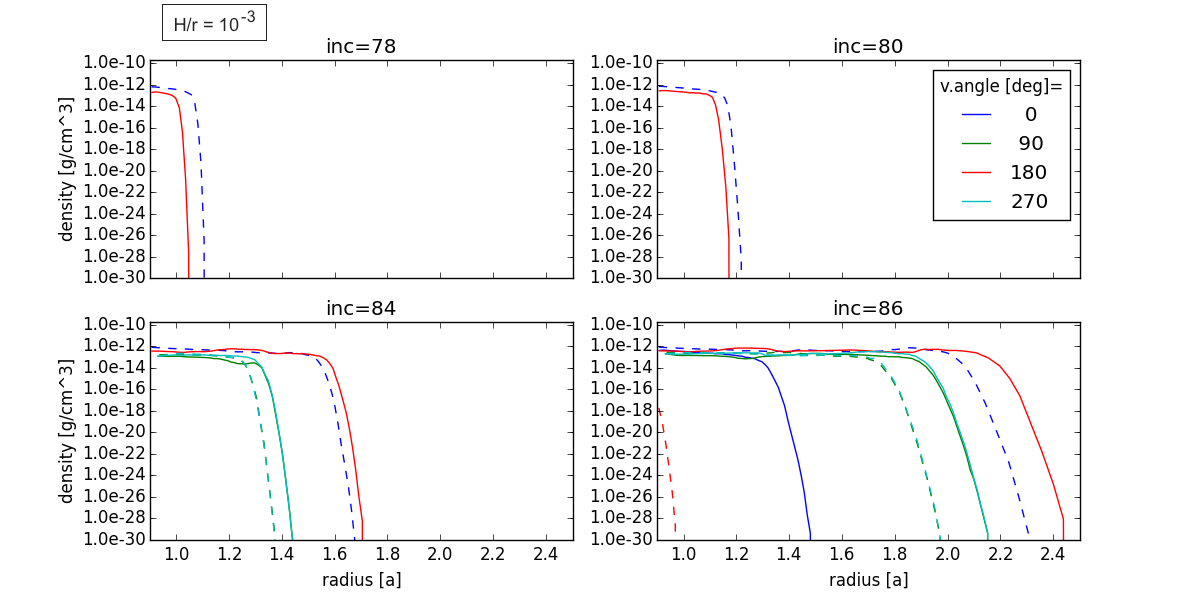
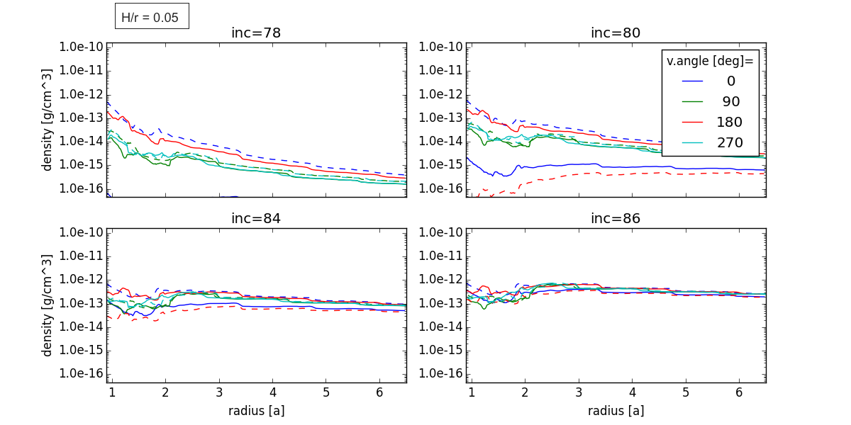
Figure 5: Mass density of gas (in g cm^-3 and in logarithmic scale) along the line of sight toward the primary (solid lines) and secondary (dashed lines) stars versus radius $r$ in the disc (in units of the binary separation $a$) for $M_{\rm dust}=10^{-12}$ M_☉. The four upper and four lower plots correspond to $H/r=10^{-3}$ and $H/r=0.05$, respectively. For each value of $H/r$, the four different plots correspond to $I=78$, $80$, $84$ and $86\degr$. In each case, the calculations are done for the viewing angles $\theta=0,90,180$ and $270\degr$. The corresponding curve is not shown when the density is too small. For the values of $H/r$ and $I$ for which the variations of the flux ressemble that of CoRoT 223992193, absorption is always produced by material located inside the disc’s inner cavity.

For the values of the parameters for which the curves displayed in figures 3 and 4 give a good fit to the CoRoT 223992193 light curve, absorption is always due to material inside the disc’s inner cavity.

In figure 6, we show the same density map as in figure 1, but with a zoom on the inner parts of the disc and with a logarithmic mapping of data to color values. The circle, of radius $r=\mbox{$r_{\rm min}$}$, shows the region which is excluded when calculating the light curves. As pointed out above, there are no dust grains in this region. It is clear from this figure that absorption comes from inside the circumbinary disc’s cavity, probably mainly from the edge of the circumstellar discs and from the streams of material which are being accreted by the stars. Figure 3 shows a “dip” in the light curves near $\theta=150\degr$. It is likely to be produced by the stream linking the circumbinary disc to the primary star, as seen in figure 6. Such a dip has been observed in CoRoT 223992193 light curve and does happen before secondary eclipse (Gillen et al. 2015), as observed here.

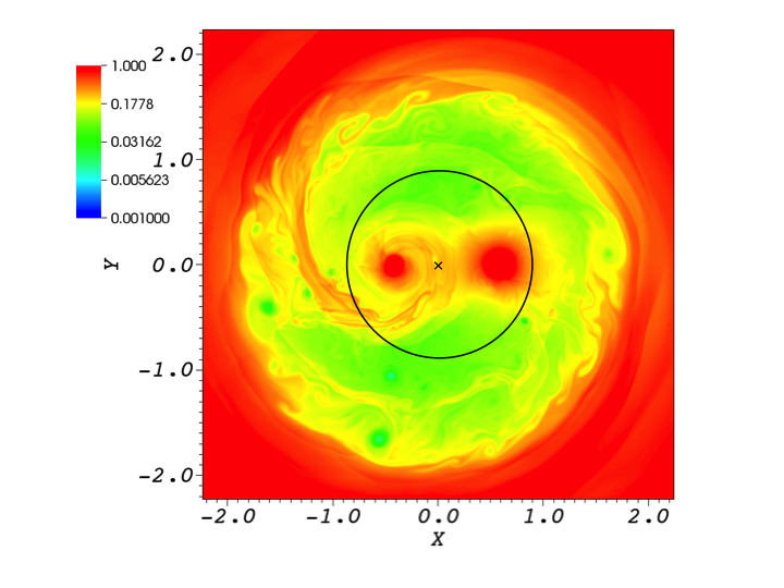
Figure 6: As in figure 1 but with a logarithmic mapping of data to color values. The cross is at the location of the centre of mass of the binary and the circle, of radius $r=\mbox{$r_{\rm min}$}=0.9$, shows the region which is excluded when calculating the light curves.

4 Summary and discussion

In this paper, we have calculated the flux received from a binary system surrounded by a circumbinary disc. The disc is modelled using two dimensional hydrodynamical simulations, and the vertical structure is derived by assuming it is isothermal. Because of the gravitational torque exerted by the binary, a cavity is created in the inner parts of the circumbinary disc. Apart from in the circumstellar discs around the stars, the surface density is much lower in this cavity than in the rest of the disc. As seen in all previous simulations of such systems, accretion streams linking the outer edge of the cavity and the circumstellar discs are present.

If the line of sight along which the system is observed has a high inclination $I$, it intersects the disc and some absorption is produced by the dust in the disc. As the system is not axisymmetric, the emergent flux varies depending on the angular coordinate in the disc along which the system is observed. We have found that variations on the order of 5–10% for $I$ close to 85$\degr$ could be obtained for a disc’s aspect ratio $H/r=10^{-3}$ and a mass of dust $M_{\rm dust}$ in the cavity above $\sim 10^{-12}$ M_☉. If $H/r=0.05$, we obtain a 5% variation only for $M_{\rm dust}=10^{-12}$ M_☉ and a rather low value of $I=78\degr$. For higher masses and/or higher values of $I$, the stars are significantly obscured. Our results show that 5–10% variability in a system where the stars are at least 90% visible at all phases can be obtained only if absorption is produced by dust located inside the disc’s inner cavity. If absorption is dominated by the parts of the disc located further away, close to or beyond the inner edge of the cavity, the stars are heavily obscured.

Although we have presented results for only one simulation of a circumbinary disc corresponding to a sound speed $c_{s}=0.3$, we have run cases with $c_{s}=0.2$ and 0.25 and checked that the light curves were very similar in all cases. When the sound speed is decreased, pressure forces are less efficient at smoothing out density enhancement, and regions of larger density become more extended. However, as we have found, the type of absorption which is observed in CoRoT 223992193 is produced in the disc’s inner cavity, and therefore the parameters that give the best fit to this system light curve do no depend on the disc’s sound speed.

To model the gas disc, we have fixed $c_{s}=0.3$, which corresponds to a gas scaleheight at hydrostatic equilibrium $H=c_{s}/\Omega_{\rm K}=0.27r^{3/2}$. However, our best fit for the CoRoT 223992193 light curve is obtained for a rather low value of $H/r=10^{-3}$. Although we have assumed in our calculation of the light curve that dust and gas were well mixed, the value of $H$ we constrain is that of the dust disc, as absorption is due solely to dust grains. In reality, the thickness of the gas and dust discs may be very different. Shi & Krolik (2015) have performed three dimensional MHD simulations of circumbinary discs, in which accretion results from the turbulence produced by the magnetorotational instability. They set up a disc with an isothermal equation of state with a sound speed $c_{s}=0.1$, corresponding to a gas disc scaleheight at hydrostatic equilibrium $H\sim 0.1r^{3/2}$. As pressure forces in the cavity are very small, the motion of the flow there is essentially ballistic and therefore particles move radially on the dynamical timescale. However, it was found that hydrostatic equilibrium still had time to be established in the vertical direction (J.–M. Shi & J. Krolik, private communication), so that the gas disc scale height in the cavity varies in the same way as in the rest of the disc. In that case, as the aspect ratio of discs around pre–main sequence stars is on the order of 0.1, the value of $H/r=10^{-3}$ needed to fit the lightcurve of CoRoT 223992193 would be that of the dust but could not be that of the gas, which would imply that dust and gas were not well mixed in the vertical direction. In the simulations performed by Shi & Krolik (2015), the flow is found to be laminar in the inner cavity. This is because the flow moves in too rapidly for magnetic instabilities to develop into turbulence (J. Krolik, private communication). In such a situation, dust grains would be expected to sedimente toward the disc midplane, which would lead to a dust disc much thinner than the gas disc (only when turbulence is present can dust grains diffuse all the way up to the disc surface and be well mixed with the gas). In that case, adopting a smaller value of $H/r$ when calculating the light curve than when modelling the disc simply amounts to ignoring the gas which is above the dust layer. It is not clear however that there would be enough time for the grains to sedimente while they are crossing the cavity. For the gas densities used in our modelling, the settling timescale is on the order of $10^{4}$–$10^{5}$ years (e.g., Dullemond & Dominik 2004). Therefore, if the particles are well mixed with the gas before entering the cavity, they would not have time to settle while flowing through the cavity. On the other hand, if the flow were not forced to be isothermal but instead proper cooling were used in the simulations, we may find that the very low density in the inner cavity enables the gas to cool down efficiently, thus reducing the scale height significantly, so that $H/r=10^{-3}$ could represent the scale height of the gas disc as well as that of the dust disc. If that were the case, our calculations would not be self–consistent, as we are using the same fixed value of $c_{s}$ in the disc and in the cavity. However, the overall $r$– and $\theta$–dependence of the gas surface density corresponding to a varying $c_{s}$ would probably not be very different from what we have been using, so that our conclusions should still be valid.

As the absorption comes almost entirely from the regions near $r_{\rm min}$, the variations of the light curves we are reproducing should have a period of about the orbital period at $r=\mbox{$r_{\rm min}$}$, which is 3.2 days. The light curves displayed in figures 3 and 4 are rather symmetric about $\theta=180\degr$, and in that case the period of the variations is actually half the orbital period. However, we have made the model symmetric by defining the inner edge of the region in which there are dust grains as a circle of radius $r=\mbox{$r_{\rm min}$}$. In reality, since the sublimation radius is different for the two stars, the geometry is more complicated and there may not be the symmetry observed in the calculations. In addition, the flow inside the cavity is likely to be very unstable with fluctuations which are not captured by our model (Shi & Krolik 2015).

References

- [2014] Cody A. M., et al., 2014, AJ, 147, 82
- [2006] de Val–Borro M., Edgar R. G., Artymowicz P. et al., 2006, MNRAS, 370, 529
- [2011] de Val–Borro M., Gahm G. F., Stempels H. C., Peplinski A., 2011, MNRAS, 413, 2679
- [2014] Gillen E. et al., 2014, A&A, 62, A50
- [2015] Gillen E. et al., 2015, submitted
- [2010] Hanawa T., Ochi Y., Ando K., 2010, ApJ, 708, 485
- [1997] Jensen E. L. N., Mathieu R. D., 1997, AJ, 114, 301
- [1979] Lin D. N. C., Papaloizou J., 1979, MNRAS, 188, 191
- [2007] Mignone A., Bodo G., Massaglia S., Matsakos T., Tesileanu O., Zanni C., Ferrari A., 2007, ApJS, 170, 228
- [1977] Paczynski B., 1977, ApJ, 216, 822
- [1977] Papaloizou J., Pringle J. E., 1977, MNRAS, 181, 441
- [2012] Shi J.–M., Krolik J. H., Lubow S. H., Hawley J. F., 2012, ApJ, 749, 118
- [2015] Shi J.–M., Krolik J. H., 2015, ApJ, 807, 131
- [2014] Stassun K. G., Feiden G. A., Torres G. 2014, NewAR, 60, 1