Volume Weighted Average Price Optimal Execution

Abstract

We study the problem of optimal execution of a trading order under Volume Weighted Average Price (VWAP) benchmark, from the point of view of a risk-averse broker. The problem consists in minimizing mean-variance of the slippage, with quadratic transaction costs. We devise multiple ways to solve it, in particular we study how to incorporate the information coming from the market during the schedule. Most related works in the literature eschew the issue of imperfect knowledge of the total market volume. We instead incorporate it in our model. We validate our method with extensive simulation of order execution on real NYSE market data. Our proposed solution, using a simple model for market volumes, reduces by $10\%$ the VWAP deviation RMSE of the standard “static” solution (and can simultaneously reduce transaction costs).

1 Introduction

Most literature on optimal execution focuses on the Implementation Shortfall (IS) objective, minimizing the execution price with respect to the market price at the moment the order is submitted. The seminal papers [BL98], [AC01] and [OW05] derive the optimal schedule for various risk preferences and market impact models. However most volume on the stock markets is traded with Volume Weighted Average Price (VWAP) orders, benchmarked to the average market price during the execution horizon [Mad02]. Using this benchmark makes the problem much more compelling from a stochastic control standpoint and prompts the development of a richer model for the market dynamics. The problem of optimal trade scheduling for VWAP execution has been studied originally [Kon02] in a static optimization setting (the schedule is fixed at the start of the day). This is intuitively suboptimal, since it ignores the new information coming as the schedule progresses. Some recent papers [HJ11] [MK12] [FW13] extend the model and incorporate the new information coming to the market but rely on the crucial assumption that the total market volume is known beforehand. Other works [BDLF08] take a different route and focus on the empirical modeling of the market volumes. A recent paper [GR13] studies the stochastic control problem including a market impact term, while the work by Li [Li13] takes a different approach and studies the optimal placement of market and limit orders for a VWAP objective. Our approach matches in complexity the most recent works in the literature ([FW13], [GR13]) with a key addition: we don’t assume that the total market volume is known and instead treat it as a random variable. We also provide extensive empirical results to validate our work.

We define the problem and all relevant variables in §2. In §3 we derive a “static” optimal trading solution. In §4 we develop a “dynamic” solution which uses the information coming from the market during the schedule in the best possible way: as our estimate of the total market volume improves we optimize our trading activity accordingly. In §5 we detail the simulations of trading we performed, on real NYSE market data, using our VWAP solution algorithms. We conclude in §6.

2 Problem formulation

We consider, from the point of view of a broker, the problem of executing a trading order issued by a client. The client decides to trade $C\in{\mbox{\bf Z}}_{+}$ shares of stock $k$ over the course of a market day. By assuming $C>0$ we restrict our analysis to “buy” orders. If we were instead interested in “sell” orders we would only need to change the appropriate signs. We don’t explore the reasons for the client’s order (it could be for rebalancing her portfolio, making new investments, etc.). The broker accepts the order and performs all the trades in the market to fulfill it. The broker has freedom in implementing the order (can decide when to buy and in what amount) but is constrained to cumulatively trade the amount $C$ over the course of the day. When the order is submitted client and broker agree on an execution benchmark price which regulates the compensation of the broker and the sharing of risk. The broker is payed by the client an amount equal to the number of shares traded times the execution benchmark, plus fees (which we neglect). In turn, the broker pays for his trading activity in the market. Some choices of benchmark prices are:

• stock price at the start of the trading schedule. This gives rise to implementation shortfall execution ([BL98], [AC01]), in which the client takes no risk (since the benchmark price is fixed);

• stock price at day close. This type of execution can misalign the broker and client objectives. The broker may try to profit from his executions by pushing the closing price up or down, using the market impact of his trades;

• Volume Weighted Average Price (VWAP), the average stock price throughout the day weighted by market volumes. This is the most common benchmark price. It encourages the broker to spread the execution evenly across the market day, minimizing market impact and detectability of the order. It assigns most risk associated with market price movements to the client, so that the broker can focus exclusively on optimizing execution.

In this paper we derive algorithms for optimal execution under the VWAP benchmark.

2.1 Definitions

We work for simplicity in discrete time. We consider a market day for a given stock, split in $T$ intervals of the same length. In the following $T$ is fixed to 390, so each interval is one minute long.

Volume

We use the word volume to denote an integer number of traded shares (either by the market as a whole or by a single agent). We define $m_{t}\in{\mbox{\bf R}}_{+}$ for $t=1,\ldots,T$, the number of shares of the stock traded by the whole market in interval $t$, which is non-negative. We note that in reality the market volumes $m_{t}$ are integer, not real numbers. This approximation is acceptable since the typical number of shares traded is much greater than 1 (if the interval length is 1 minute or more) so the integer rounding error is negligible. These market volumes are distributed according to a joint probability distribution

$$f_{m_{1:T}}(m_{1},\ldots,m_{T}).$$

In §5.2 we propose a model for this joint distribution. We also define the total daily volume

$$V=\sum_{t=1}^{T}m_{t}$$

We call $u_{t}\in{\mbox{\bf R}}_{+}$ the number of shares of the stock that our broker trades in interval $t$, for $t=1,\ldots,T$. (Again we assume that the volumes are large enough so the rounding error is negligible.) By regulations these must be non-negative, so that all trades performed by the broker as part of the order have the same sign.

Price

Let $p_{t}\in{\mbox{\bf R}}_{++}$ for $t=1,\ldots,T$ be the average market price for the stock in interval $t$. This is defined as the VWAP of all trades over interval $t$. (If during interval $t$ there are $N_{t}>0$ trades in the market, each one with volume $\omega_{i}\in{\mbox{\bf Z}}_{++}$ and price $\pi_{i}\in{\mbox{\bf R}}_{++}$, then $p_{t}={\sum_{i=1}^{N_{t}}\omega_{i}\pi_{i}}/{\sum_{i=1}^{N_{t}}\omega_{i}}.$) If there are no trades during interval $t$ then $p_{t}$ is undefined and in practice we set it equal to the last available period price. We model this price process as a geometric random walk with zero drift. The initial price $p_{0}$ is a known constant. Then the price increments $\eta_{t}\equiv\frac{p_{t}-p_{t-1}}{p_{t-1}}$ for $t=1,\ldots,T$ are independent and distributed as

$$\eta_{t}\sim\mathcal{N}(0,\sigma_{t}),$$

where $\mathcal{N}$ is the Gaussian distribution. The period volatilities $\sigma_{t}\in{\mbox{\bf R}}_{+}$ for $t=1,\ldots,T$ are constants known from the start of the market day. We define the market VWAP price as

$$p_{\text{VWAP}}=\frac{\sum_{t=1}^{T}m_{t}p_{t}}{V}.$$ (1)

Transaction costs

We model the transaction costs by introducing the effective price $\hat{p}_{t}$, defined so that the whole cost of the trade at interval $t$ is $u_{t}\hat{p}_{t}$. Our model captures instantaneous transaction costs, in particular the cost of the bid-ask spread, not the cost of long-term market impact. (For a detailed literature review on transaction costs and market impact see [BFL09].) Let $s_{t}\in{\mbox{\bf R}}_{++}$ be the average fractional (as ratio of the stock price) bid-ask spread in period $t$. We assume the broker trades the volume $u_{t}$ using an optimized trading algorithm that mixes optimally market and limit orders. The cost or proceeding per share of a buy market order is on average $p_{t}(1+{s_{t}}/{2})$ while for a limit order it is on average $p_{t}(1-{s_{t}}/{2})$. Let $u_{\text{LO}}$ and $u_{\text{MO}}$ be the portions of $u_{t}$ executed via limit orders and market orders, respectively, so that $u_{\text{LO}}+u_{\text{MO}}=u_{t}$. We require that the algorithm uses trades of the same sign, so $u_{\text{LO}}$, $u_{\text{MO}}$, and $u_{t}$ are all non-negative (consistently with the constraint we introduce in §2.3). We assume that the fraction of market orders over the traded volume is proportional to the participation rate, defined as ${u_{t}}/{m_{t}}$. So

$$\frac{u_{\text{MO}}}{u_{t}}=\frac{\alpha}{2}\frac{u_{t}}{m_{t}}$$

where the proportionality factor $\alpha\in{\mbox{\bf R}}_{+}$ depends on the specifics of the trading algorithm used. This is a reasonable assumption, especially in the limit of small participation rate. The whole cost or proceedings of the trade is

$$u_{t}\hat{p}_{t}=p_{t}\left(u_{\text{LO}}\left(1-\frac{s_{t}}{2}\right)+u_{\text{MO}}\left(1+\frac{s_{t}}{2}\right)\right)$$

which implies

$$\hat{p}_{t}=p_{t}\left(1-\frac{s_{t}}{2}+\alpha\frac{s_{t}}{2}\frac{u_{t}}{m_{t}}\right).$$ (2)

We thus have a simple model for the effective price $\hat{p}_{t}$, linear in $u_{t}$. This gives rise to quadratic transaction costs, a reasonable approximation for the stock markets ([BFL09], [LFM03]).

2.2 Problem objective

Consider the cash flow for the broker, equal to the payment he receives from the client minus the cost of trading

$$Cp_{\text{VWAP}}-\sum_{t=1}^{T}u_{t}\hat{p}_{t}.$$

In practice there would also be fees but we neglect them. The trading industry usually defines the slippage as the negative of this cash flow. It represents the amount by which the order execution price misses the benchmark. (The choice of sign is conventional so that the optimization problem consists in minimizing it). We instead define the slippage as

$$S\equiv\frac{\sum_{t=1}^{T}u_{t}\hat{p}_{t}-Cp_{\text{VWAP}}}{Cp_{\text{VWAP}}},$$ (3)

normalizing by the value of the order. We need this in order to compare the slippage between different orders. By substituting the expressions defined above we get

$$S=\left.\left(\sum_{t=1}^{T}\left[u_{t}p_{t}\left(1-\frac{s_{t}}{2}+\alpha\frac{s_{t}}{2}\frac{u_{t}}{m_{t}}\right)\right]-C\frac{\sum_{t=1}^{T}m_{t}p_{t}}{V}\right)\right/{Cp_{\text{VWAP}}}=\\ \sum_{t=1}^{T}\left[\frac{p_{t}}{p_{\text{VWAP}}}\left(\frac{u_{t}}{C}-\frac{m_{t}}{V}\right)\right]+\sum_{t=1}^{T}\frac{p_{t}s_{t}}{2p_{\text{VWAP}}}\left(\alpha\frac{u^{2}_{t}}{Cm_{t}}-\frac{u_{t}}{C}\right)\simeq\\ \sum_{t=1}^{T-1}\left[\eta_{t+1}\left(\frac{\sum_{\tau=1}^{t}m_{\tau}}{V}-\frac{\sum_{\tau=1}^{t}u_{\tau}}{C}\right)\right]+\sum_{t=1}^{T}\frac{s_{t}}{2}\left(\alpha\frac{u^{2}_{t}}{Cm_{t}}-\frac{u_{t}}{C}\right)$$ (4)

where we used the two approximations (both first order, reasonable on a trading horizon of one day)

$$\frac{p_{t}-p_{t-1}}{p_{\text{VWAP}}} \simeq \frac{p_{t}-p_{t-1}}{p_{t-1}}=\eta_{t}$$ (5)

$$\frac{p_{t}s_{t}}{p_{\text{VWAP}}} \simeq s_{t}.$$ (6)

We model the broker as a standard risk-averse agent, so that the objective function is to minimize

$$\mathop{\bf E{}}S+\lambda\mathop{\bf var}(S)$$

for a given risk-aversion parameter $\lambda\geq 0$. These expectation and variance operators apply to all sources of randomness in the system, i.e., the market volumes $m$ and market prices $p$, which are independent under our model. The expected value of the slippage is

$$\mathop{\bf E{}}_{m,p}S=\mathop{\bf E{}}_{m}\mathop{\bf E{}}_{p}S=\mathop{\bf E{}}_{m}\left[\sum_{t=1}^{T}\frac{{s}_{t}}{2}\left(\alpha\frac{u^{2}_{t}}{Cm_{t}}-\frac{u_{t}}{C}\right)\right]$$ (7)

since the price increments have zero mean. Note that we leave expressed the expectation over market volumes. The variance of the slippage is

$$\mathop{\bf var}_{m,p}S=\mathop{\bf E{}}_{m,p}\left[\left(S-\mathop{\bf E{}}_{m,p}S\right)^{2}\right]=\mathop{\bf E{}}_{m,p}S^{2}-\left(\mathop{\bf E{}}_{m,p}S\right)^{2}=\\ \mathop{\bf E{}}_{m}\mathop{\bf E{}}_{p}S^{2}-\left(\mathop{\bf E{}}_{m}\mathop{\bf E{}}_{p}S\right)^{2}-\mathop{\bf E{}}_{m}(\mathop{\bf E{}}_{p}S)^{2}+\mathop{\bf E{}}_{m}(\mathop{\bf E{}}_{p}S)^{2}=\mathop{\bf E{}}_{m}\mathop{\bf var}_{p}(S)+\mathop{\bf var}_{m}(\mathop{\bf E{}}_{p}S).$$ (8)

The first term is

$$\mathop{\bf E{}}_{m}\mathop{\bf var}_{p}(S)=\mathop{\bf E{}}_{m}\mathop{\bf E{}}_{p}\left[\left(\sum_{t=1}^{T-1}\eta_{t+1}\left(\frac{\sum_{\tau=1}^{t}m_{t}}{V}-\frac{\sum_{\tau=1}^{t}u_{t}}{C}\right)\right)^{2}\right]=\\ \mathop{\bf E{}}_{m}\left[\sum_{t=1}^{T-1}{\sigma}^{2}_{t+1}\left(\frac{\sum_{\tau=1}^{t}m_{t}}{V}-\frac{\sum_{\tau=1}^{t}u_{t}}{C}\right)^{2}\right]$$ (9)

which follows from independence of the price increment. The second term is

$$\mathop{\bf var}_{m}(\mathop{\bf E{}}_{p}S)=\mathop{\bf var}_{m}\left(\sum_{t=1}^{T}\frac{{s}_{t}}{2}\left(\alpha\frac{u^{2}_{t}}{Cm_{t}}-\frac{u_{t}}{C}\right)\right).$$ (10)

We drop the second term and only keep the first one, so that the resulting optimization problem is tractable. We motivate this by assuming, as in [FW13], that the second term of the variance is negligible when compared to the first. This is validated ex-post by our empirical studies in §5. We thus get

$$\mathop{\bf E{}}_{m,p}S+\lambda\mathop{\bf var}_{m,p}(S)\simeq\sum_{t=1}^{T}\mathop{\bf E{}}_{m}\left[\frac{{s}_{t}}{2}\left(\alpha\frac{u^{2}_{t}}{Cm_{t}}-\frac{u_{t}}{C}\right)+\lambda{\sigma}_{t}^{2}\left(\frac{\sum_{\tau=1}^{t-1}m_{t}}{V}-\frac{\sum_{\tau=1}^{t-1}u_{t}}{C}\right)^{2}\right].$$ (11)

We note that the objective function separates in a sum of terms per each time step, a key feature we will use to apply the dynamic programming optimization techniques in §4.

2.3 Constraints

We consider the constraints that apply to the optimization problem. The optimization variables are $u_{t}$ for $t=1,\ldots,T$. We require that the executed volumes sum to the total order size C

$$\sum_{t=1}^{T}u_{t}=C.$$ (12)

We then impose that all trades have positive sign (buys)

$$u_{t}\geq 0,\ \ t=1,\ldots,T.$$ (13)

(If we were executing a sell order, $C<0$, we would have all $u_{t}\leq 0$.) This is a regulatory requirement for institutional brokers in most markets, essentially as a precaution against market manipulation. It is a standard constraint in the literature about VWAP execution.

2.4 Optimization paradigm

The price increments $\eta_{t}$ and market volumes $m_{t}$ are stochastic. The volumes $u_{t}$ instead are chosen as the solution of an optimization problem. This problem can be cast in several different ways. We define the information set $I_{t}$ available at time $t$

$$I_{t}\equiv\{(p_{1},m_{1},u_{1}),\ldots,(p_{t-1},m_{t-1},u_{t-1})\}.$$ (14)

By causality, we know that when we choose the value of $u_{t}$ we can use, at most, the information contained in $I_{t}$. In §3 we formulate the optimization problem and provide an optimal solution for the variables $u_{t}$ in the case we do not access anything from the information set $I_{t}$ when choosing $u_{t}$. The $u_{t}$ are chosen using only information available before the trading starts. We call this a static solution (or open loop in the language of control). In §4 instead we develop an optimal policy which can be seen as a sequence of functions $\psi_{t}$ of the information set available at time $t$

$$u_{t}=\psi_{t}(I_{t}).$$

We develop it in the framework on dynamic programming and we call it dynamic solution (or closed loop).

3 Static solution

We consider a procedure to solve the problem described in §2 without accessing the information sets $I_{t}$. We call this solution static since it is fixed at the start of the trading period. (It is computed using only information available before the trading starts.) This is the same assumption of [Kon02] and corresponds to the approach used by many practitioners. Our model is however more flexible than [Kon02], it incorporates variable bid-ask spread and a sophisticated transaction cost model. Still, it has an extremely simple numericaly solution that leverages convex optimization [BV09] theory and software.

We start by the optimization problem with objective function (11) and the two constraints (12) and (13)

$$\begin{array}[]{ll}\text{minimize}_{u}&\mathop{\bf E{}}_{m,p}S+\lambda\mathop{\bf var}_{m,p}(S)\\ \mbox{s.t.}&\sum_{t=1}^{T}u_{t}=C\\ &u_{t}\geq 0,\quad t=1,\ldots,T.\\ \end{array}$$

We remove a constant term from the objective and write the problem in the equivalent form

$$\begin{array}[]{ll}\text{minimize}_{u}&\sum_{t=1}^{T}\left[\frac{{s}_{t}}{2C}\left(\alpha{u^{2}_{t}\kappa_{t}}-{u_{t}}\right)+\lambda{\sigma}_{t}^{2}\left({\left(\frac{\sum_{\tau=1}^{t-1}u_{t}}{C}\right)}^{2}-2M_{t}\frac{\sum_{\tau=1}^{t-1}u_{t}}{C}\right)\right]\\ \mbox{s.t.}&\sum_{t=1}^{T}u_{t}=C\\ &u_{t}\geq 0,\quad t=1,\ldots,T\\ \end{array}$$ (15)

where $M_{t}$ and $\kappa_{t}$ are the constants

$$M_{t}=\mathop{\bf E{}}_{m}\left[\frac{\sum_{\tau=1}^{t-1}m_{t}}{V}\right],\quad\kappa_{t}=\mathop{\bf E{}}_{m}\left[\frac{1}{m_{t}}\right]$$

for $t=1,\ldots,T$. In this form, the problem is a standard quadratic program [BV09] and can be solved efficiently by open-source solvers such as ECOS [DCB13] using a symbolic convex optimization suite like CVX [GB14] or CVXPY [DCB14].

3.1 Constant spread

We consider the special case of constant spread, $s_{1}=\cdots=s_{T}$, which leads to a great simplification of the solution. The convex problem (15) has the form

$$\begin{array}[]{ll}\text{minimize}_{u}&\sum_{t=1}^{T}\frac{{s}_{t}}{2C}\left(\alpha{u^{2}_{t}\kappa_{t}}-u_{t}\right)+\lambda\left(\sum_{t=1}^{T}{\sigma}_{t}^{2}\left(U_{t}^{2}-2M_{t}{U_{t}}/{C}\right)\right)\equiv\phi(u)+\lambda\psi(u)\\ \mbox{s.t.}&u\in\mathcal{C}\\ \end{array}$$

where $U_{t}={\sum_{\tau=1}^{t-1}u_{t}}/{C}$ for each $t=1,\ldots,T$, and $\mathcal{C}$ is the convex feasible set. We separate the problem into two subproblems considering each of the two terms of the objective. The first one is

$$\begin{array}[]{ll}\text{minimize}_{u}&\phi(u)\\ \mbox{s.t.}&u\in\mathcal{C}\\ \end{array}$$

which is equivalent to (since the spread is constant and $\alpha>0$)

$$\begin{array}[]{ll}\text{minimize}_{u}&\sum_{t=1}^{T}u^{2}_{t}\kappa_{t}\\ \mbox{s.t.}&u\in\mathcal{C}\\ \end{array}$$

The optimal solution is ([BV09], Lagrange duality)

$$u_{t}^{\star}=C\frac{1/\kappa_{t}}{\sum_{t=1}^{T}1/\kappa_{t}},\quad t=1,\ldots,T.$$

We approximate $\kappa_{t}=\mathop{\bf E{}}_{m}\left[{1}/{m_{t}}\right]\simeq{1}/{\mathop{\bf E{}}_{m}[m_{t}]}$ and thus

$$u_{t}^{\star}\simeq C\frac{\mathop{\bf E{}}_{m}[m_{t}]}{\sum_{t=1}^{T}\mathop{\bf E{}}_{m}[m_{t}]}\simeq C\mathop{\bf E{}}_{m}\left[\frac{m_{t}}{V}\right],\quad t=1,\ldots,T.$$

The second problem is

$$\begin{array}[]{ll}\text{minimize}_{u}&\psi(u)\equiv\sum_{t=1}^{T}{\sigma}_{t}^{2}\left(U_{t}^{2}-2M_{t}{U_{t}}/{C}\right)\\ &u\in\mathcal{C}\\ \end{array}$$

we choose the $U_{t}$ such that ${\sigma}_{t}^{2}\left(U_{t}-M_{t}\right)=0$ so $U_{t}=M_{t}$ for $t=1,\ldots,T$. The values of $u_{1},\ldots,u_{T-1}$ are thus fixed, and we choose the final volume $u_{T}$ so that $u_{T}=C-CU_{T}$. The first order condition of the objective function is satisfied, and these values of $u_{1},\ldots,u_{T}$ are feasible (since $M_{t}$ is non-decreasing in $t$ and $M_{T}\leq 1$). It follows that this is an optimal solution, it has values $u_{t}^{\star}=C\mathop{\bf E{}}_{m}\left[{m_{t}}/{V}\right]$ for $t=1,\ldots,T$.

Consider now the original problem. Its objective is a convex combination (apart from a constant factor) of the objectives of two convex problem above and all three have the same constraints set. Since the two subproblems share an optimal solution $u^{\star}$, it follows that $u^{\star}$ is also an optimal solution for the combined problem. Thus, an the optimal solution of (15) in the case of constant spread is

$$u_{t}^{\star}=C\mathop{\bf E{}}_{m}\left[\frac{m_{t}}{V}\right]\quad t=1,\ldots,T.$$ (16)

This is equivalent to the solution derived in [Kon02] and is the standard in the brokerage industry. In our model this solution arises as the special case of constant spread, in general we could derive more sophisticated static solutions. We also note that we introduced the approximation $\kappa_{t}=\mathop{\bf E{}}_{m}\left[{1}/{m_{t}}\right]\simeq{1}/{\mathop{\bf E{}}_{m}[m_{t}]}$. (In practice, estimating $\mathop{\bf E{}}_{m}\left[{1}/{m_{t}}\right]$ would require a more sophisticated model of market volumes than $\mathop{\bf E{}}_{m}\left[{m_{t}}/{V}\right]$). We thus expect to lose some efficiency in the optimization of the trading costs. However, with respect to the minimization of the variance of $S$ (if $\lambda\to\infty$ or $s=0$), this solution is indeed optimal. In the following we compare the performances of (16) and of the dynamic solution developed in §4.

4 Dynamic solution

We develop a solution of the problem that uses all the information available at the time each decision is made, i.e., a sequence of functions $\psi_{t}(I_{t})$ where $I_{t}$ is the information set available at time $t$ (as defined in (14)). We work in the framework of Dynamic Programming (DP) [Ber95], summarized in §4.1. In particular we fit our problem in the special case of linear dynamics and quadratic costs, described in §4.2. However we can’t apply standard DP because the random shocks affecting the system at different times are not conditionally independent (the market volumes have a joint distribution). We instead use the approximate procedure of [SBZ10], summarized in §4.3. In §4.4 we finally write our optimization problem, defining the state, action and costs, and in §4.5 we derive its solution.

4.1 Dynamic programming

We summarize here the standard formalism of dynamic programming, following [Ber95]. Suppose we have a state variable $x_{t}\in\mathcal{X}$ defined for $t=1,...,T+1$ with $x_{1}$ known. Our decision variables are $u_{t}\in\mathcal{U}$ for $t=1,...,T$ and each $u_{t}$ is chosen as a function of the current state, $u_{t}=\mu_{t}(x_{t})$. (We use the same symbol as the volumes traded at time $t$ since in the following they coincide.) The randomness of the system is modeled by a series of IID random variables $w_{t}\in\mathcal{W}$, for $t=1,...,T$. The dynamics is described by a series of functions

$$x_{t+1}=f_{t}(x_{t},u_{t},w_{t}),$$

at every stage we incur the cost

$$g_{t}(x_{t},u_{t},w_{t}),$$

and at the end of the decision process we have a final cost

$$g_{T+1}(x_{T+1}).$$

Our objective is to minimize

$$J=\mathop{\bf E{}}\left[\sum_{t=1}^{T}g_{t}(x_{t},u_{t},w_{t})+g_{T+1}(x_{T+1})\right].$$

We solve the problem by backward induction, defining the cost-to-go function $v_{t}$ at each time step $t$

$$v_{t}(x)=\min_{u}\mathop{\bf E{}}[g_{t}(x,u,w_{t})+v_{t+1}(f_{t}(x,u,w_{t}))],\quad t=1,\ldots,T.$$ (17)

This recursion is known as Bellman equation. The final condition is fixed by

$$v_{T+1}(\cdot)=g_{T+1}(\cdot).$$

It follows that the optimal action at time $t$ is given by the solution

$$u_{t}=\mathop{\rm argmin}_{u}\mathop{\bf E{}}[g_{t}(x_{t},u,w_{t})+v_{t+1}(f_{t}(x_{t},u,w_{t}))].$$ (18)

In general, these equations are not solvable since the iteration that defines the functions $v_{t}$ requires an amount of computation exponential in the dimension of the state space, action space, and number of time steps (curse of dimensionality). However some special forms of this problem have closed form solutions. We see one in the following section.

4.2 Linear-quadratic stochastic control

Whenever the dynamics functions $f_{t}$ are stochastic affine and the cost functions are stochastic quadratic, the problem of §4.1 has an analytic solution [BLR12]. We call this Linear-Quadratic Stochastic Control (LQSC). We define the state space $\mathcal{X}={\mbox{\bf R}}^{n}$, the action space $\mathcal{U}={\mbox{\bf R}}^{m}$ for some $n,m>0$. The disturbances are independent with known distributions and belong to a general set $\mathcal{W}$. For $t=1,\ldots,T$ the system dynamics is described by

$$x_{t+1}=f_{t}(x_{t},u_{t},w_{t})=A_{t}(w_{t})x_{t}+B_{t}(w_{t})u_{t}+c_{t}(w_{t}),\ \ t=1,...,T$$

with matrix functions $A_{t}(\cdot):\mathcal{W}\to{\mbox{\bf R}}^{n\times n}$, $B_{t}(\cdot):\mathcal{W}\to{\mbox{\bf R}}^{n\times m}$, and $c_{t}(\cdot):\mathcal{W}\to{\mbox{\bf R}}^{n}$. The stage costs are

$$g_{t}(x_{t},u_{t},w_{t})=x_{t}^{T}Q_{t}(w_{t})x_{t}+q_{t}(w_{t})^{T}x_{t}+u_{t}^{T}R_{t}(w_{t})u_{t}+r_{t}(w_{t})^{T}u_{t}$$

with matrix functions $Q_{t}(\cdot):\mathcal{W}\to{\mbox{\bf R}}^{n\times n}$, $q_{t}(\cdot):\mathcal{W}\to{\mbox{\bf R}}^{n}$, $R_{t}(\cdot):\mathcal{W}\to{\mbox{\bf R}}^{m\times m}$, and $r_{t}(\cdot):\mathcal{W}\to{\mbox{\bf R}}^{m}$. The final cost is a quadratic function of the final state

$$g_{T+1}(x_{T+1})=x_{T+1}^{T}Q_{T+1}x_{T+1}+q_{T+1}^{T}x_{T+1}.$$

The main result of the theory on linear-quadratic problems [Ber95] is that the optimal policy $\mu_{t}(x_{t})$ is a simple affine function of the problem parameters and can be obtained analytically

$$\mu_{t}(x_{t})=K_{t}x_{t}+l_{t},\ \ t=0,...,T-1,$$ (19)

where $K_{t}\in{\mbox{\bf R}}^{m\times n}$ and $l_{t}\in{\mbox{\bf R}}^{m}$ depend on the problem parameters. In addition, the cost-to-go function is a quadratic function of the state

$$v_{t}(x_{t})=x_{t}^{T}D_{t}x_{t}+d_{t}^{T}x_{t}+b_{t}$$ (20)

where $D_{t}\in{\mbox{\bf R}}^{n\times n}$, $d_{t}\in{\mbox{\bf R}}^{n}$, and $b_{t}\in{\mbox{\bf R}}$ for $t=1,\ldots,T$. We derive these results solving the Bellman equations (17) by backward induction. These are known as Riccati equations, reported in Appendix A.1.

4.3 Conditionally dependent disturbances

We now consider the case in which the disturbances are not independent, and we can’t apply the Bellman iteration of §4.1. Specifically, we assume that the disturbances have a joint distribution described by a density function

$$f_{w}(\cdot):\mathcal{W}\times\cdots\times\mathcal{W}\to[0,1].$$

One approach to solve this problem is to augment the state $x_{t}$, by including the disturbances observed up to time $t$. This causes the computational complexity of the solution to grow exponentially with the increased dimensionality (curse of dimensionality). Some approximate dynamic programming techniques can be used to solve the augmented problem [Ber95] [Pow07]. We take instead the approximate approach developed in [SBZ10], called shrinking-horizon dynamic programming (SHDP), which performs reasonably well in practice and leads to a tractable solution. (It can be seen as an extension of model predictive control, known to perform well in a variety of scenarios [Bem06] [KH06] [MWB11] [BMOW13]).

We now summarize the approach. Assume we know the density of the future disturbances $w_{t},\ldots,w_{T}$ conditioned on the observed ones

$$f_{w|{t}}(w_{t},\ldots,w_{T}):\mathcal{W}\times\cdots\times\mathcal{W}\to[0,1].$$

(If $t=1$ this is the unconditional density.) We derive the marginal density of each future disturbance, by integrating over all others,

$$\hat{f}_{w_{t}|t}(w_{t}),\ldots,\hat{f}_{w_{T}|t}(w_{T}).$$

We use the product of these marginals to approximate the density of the future disturbances, so they all are independent. We then compute the cost-to-go functions with backwards induction using the Bellman equations (17) and (18), where the expectations over each disturbance $w_{\tau}$ are taken on the conditional marginal density $\hat{f}_{w_{\tau}|t}$. The equations (17) for the cost-to-go function become (note the subscript ${\cdot|t}$)

$$v_{\tau|t}(x)=\min_{u}\mathop{\bf E{}}_{\hat{f}_{w_{\tau}|t}}[g_{\tau}(x,u,w_{\tau})+v_{\tau+1|t}(f_{\tau}(x,u,w_{\tau}))],$$ (21)

for all times $\tau=t,\ldots,T$, with the usual final condition. Similarly, the equations (18) for the optimal action become

$$u_{t}=\mathop{\rm argmin}_{u}\mathop{\bf E{}}_{\hat{f}_{w_{t}|t}}[g_{t}(x_{t},u,w_{t})+v_{t+1|t}(f_{t}(x_{t},u,w_{t}))]$$ (22)

for all times $\tau=t,\ldots,T$. We only use the solution $u_{t}$ at time $t$. In fact when we proceed to the next time step $t+1$ we rebuild the whole sequence of cost-to-go functions $v_{t+1|t+1}(x),\ldots,v_{T|t+1}(x)$ using the updated marginal conditional densities and then solve (22) to get $u_{t+1}$. With this framework we can solve the VWAP problem we developed in §2.

4.4 VWAP problem as LQSC

We now formulate the problem described in §2 in the framework of §4.2. For $t=1,\ldots,T+1$ we define the state as:

$$x_{t}=\left(\begin{array}[]{c}\sum_{\tau=1}^{t-1}u_{\tau}\\ \sum_{\tau=1}^{t-1}m_{\tau}\end{array}\right),$$ (23)

so that $x_{1}=(0,0)$. The action is $u_{t}$, the volume we trade during interval $t$, as defined in §2.

The disturbance is

$$w_{t}=\left(\begin{array}[]{c}m_{t}\\ V\end{array}\right)$$ (24)

where the second element is the total market volume $V=\sum_{t=1}^{T}m_{t}$. With this definition the disturbances are not conditionally independent. In §4.5 we study their joint and marginal distributions. We note that $V$, the second element of each $w_{t}$, is not observed after time $t$. (The theory we developed so far does not require the disturbances $w_{t}$ to be observed, the Bellman equations only need expected values of functions of $w_{t}$.) For $t=1,...,T$ the state transition consists in

$$x_{t+1}=x_{t}+\left(\begin{array}[]{c}{u_{t}}\\ {m_{t}}\end{array}\right).$$

So that the dynamics matrices are

$$A_{t}(w_{t}) = \left(\begin{array}[]{cc}1&0\\ 0&1\\ \end{array}\right)\equiv I,$$

$$B_{t}(w_{t}) = \left(\begin{array}[]{c}1\\ 0\\ \end{array}\right)\equiv e_{1},$$

$$c_{t}(w_{t}) = \left(\begin{array}[]{c}0\\ m_{t}\\ \end{array}\right).$$

The objective funtion (11) can be written as $\mathop{\bf E{}}_{m}\sum_{t=1}^{T}g_{t}(x_{t},u_{t},w_{t})$ where each stage cost is given by

$$g_{t}(x_{t},u_{t},w_{t})=\frac{{s}_{t}}{2}\left(\alpha\frac{u_{t}^{2}}{Cm_{t}}-\frac{u_{t}}{C}\right)+\lambda{\sigma}_{t}^{2}x_{t}^{T}\left(\begin{array}[]{cc}\frac{1}{C^{2}}&-\frac{1}{CV}\\ -\frac{1}{CV}&\frac{1}{V^{2}}\\ \end{array}\right)x_{t}.$$

The quadratic cost function terms are thus

$$Q_{t}(w_{t}) = \lambda\sigma_{t}^{2}\left(\begin{array}[]{cc}\frac{1}{C^{2}}&-{1}/{CV}\\ -{1}/{CV}&{1}/{V^{2}}\\ \end{array}\right)$$

$$q_{t}(w_{t}) = 0$$

$$R_{t}(w_{t}) = \frac{\alpha s_{t}}{2Cm_{t}}$$

$$r_{t}(w_{t}) = -\frac{s_{t}}{2C}$$

for $t=1,\ldots,T$. The constraint that the total executed volume is equal to $C$ imposes the last action

$$u_{T}=\mu_{T}(x_{T})=C-\sum_{t=1}^{T-1}u_{t},\equiv K_{T}x_{t}+l_{t}$$

with

$$K_{T} = -e_{1}^{T}$$

$$l_{T} = C.$$

This in turn fixes the value function at time $T$

$$v_{T}(x_{T})=\mathop{\bf E{}}g_{T}(x_{T},K_{T}x_{t}+l_{t},w_{t}),$$ (29)

so we can treat $x_{T}$ as our final state and only consider the problem of choosing actions up to $u_{T-1}$. We are left with the constraint $u_{t}\geq 0$ for $t=1,\ldots,T$. Unfortunately this can not be enforced in the LQSC formalism. We instead take the approximate dynamic programming approach of [KB14]. We allow $u_{t}$ to get negative sign and then project it on the set of feasible solutions. For every $t=1,\ldots,T$ we compute

$$\max(u_{t},0)$$

and use it, instead of $u_{t}$, for our trading schedule. This completes the formulation of our optimization problem into the linear-quadratic stochastic control framework. We now focus on its solution, using the approximate approach of §4.3.

4.5 Solution in SHDP

We provide an approximate solution of the problem defined in §4.4 using the framework of shinking-horizon dynamic programming (summarized in §4.3). Consider a fixed time $t=1,\ldots,T-1$. We note that (unlike the assumption of [SBZ10]) we do not observe the sequence of disturbances $w_{1},\ldots,w_{t-1}$, because the total volume $V$ is not known until the end of the day. We only observe the sequence of market volumes $m_{1},\ldots,m_{t-1}$.

If $f_{m}(m_{1},\ldots,m_{T})$ is the joint distribution of the market volumes, then the joint distribution of the disturbances is

$$f_{w}(w_{1},\ldots,w_{t})=f_{m}(e_{1}^{T}w_{1},\ldots,e_{1}^{T}w_{T})\times\mathbf{1}_{\{e_{2}^{T}w_{1}=V\}}\times\cdots\times\mathbf{1}_{\{e_{2}^{T}w_{T}=V\}}\times\mathbf{1}_{\{V=\sum_{\tau=1}^{T}e_{1}^{T}w_{\tau}\}}$$

where $e_{1}=(1,0)$, $e_{2}=(0,1)$, and the function $\mathbf{1}_{\{\cdot\}}$ has value 1 when the condition is true and 0 otherwise. We assume that our market volumes model also provides the conditional density $f_{m|t}(m_{t},\ldots,m_{T})$ of $m_{t},\ldots,m_{T}$ given $m_{1},\ldots,m_{t-1}$. The conditional distribution of $V$ given $m_{1},\ldots,m_{t-1}$ is

$$f_{V|t}(V)=\int\cdots\int f_{m|t}(m_{t},\ldots,m_{T})\mathbf{1}_{\{V=\sum_{\tau=1}^{T}m_{\tau}\}}dm_{t}\cdots dm_{T}$$

(where the first $t-1$ market volumes are constants and the others are integration variables). Let the marginal densities be

$$\hat{f}_{m_{t}|t}(m_{t}),\ldots,\hat{f}_{m_{T}|t}(m_{T}).$$

The marginal conditional densities of the disturbances are thus

$$\hat{f}_{w_{\tau}|t}(\cdot)=\hat{f}_{m_{\tau}|t}(\cdot)\times f_{V|t}(\cdot)$$ (30)

for $\tau=t,\ldots,T$.

We use these to apply the machinery of §4.3, solve the Bellman equations and obtain the suboptimal SHDP policy at time $t$. We compute the whole sequence of cost-to-go functions and policies at times $\tau=t,\ldots,T$. The cost-to-go functions are

$$v_{\tau|t}(x_{\tau})=x_{\tau}^{T}D_{\tau|t}x_{\tau}+d_{\tau|t}x_{\tau}+b_{\tau|t}$$ (31)

for $\tau=t,\ldots,T-1$. The only difference with equation (20) is the condition $|t$ in the subscript, because expected values are taken over the marginal conditional densities $\hat{f}_{w_{\tau}|t}(\cdot)$. Similarly, the policies are

$$\mu_{\tau|t}(x_{\tau})=K_{\tau|t}x_{\tau}+l_{\tau|t}$$ (32)

for $\tau=t,\ldots,T-1$. We report the equations for this recursion in Appendix A.2. At every time step $t$ we compute the whole sequence of cost-to-go and policies, in order to get the optimal action

$$u_{t}^{\star}=\mu_{t|t}(x_{t})=K_{\tau|t}x_{\tau}+l_{\tau|t}.$$ (33)

We then move to the next time step and repeat the whole process. If we are not interested in computing the cost-to-go $v_{t|t}(x_{t})$ the equations simplify somewhat (we disregard large part of the recursion and only compute what we need). We develop these simplified formulas in Appendix A.3.

5 Empirical results

We study the performance of the static solution of §3 versus the dynamic solution of §4 by simulating execution or stock orders, using real NYSE market price and volume data. We describe in §5.1 the dataset and how we process it. The dynamic solution requires a model for the joint distribution of market volumes, here we use a simple model, explained in §5.2. (We expect that a more sophisticated model for market volumes would improve the solution performance significantly.) In §5.3 we describe the “rolling testing” framework in which we operate. Our procedure is made up of two parts: the historical estimation of model parameters, explained in §5.4, and the actual simulation of order execution, in §5.5. Finally in §5.6 we show our aggregate results.

5.1 Data

We simulate execution on data from the NYSE stock market. Specifically, we use the $K=30$ different stocks which make up the Dow Jones Industrial Average (DJIA), on $N=60$ market days corresponding to the last quarter of 2012, from September 24 to December 20 (we do not consider the last days of December because the market was either closed or had reduced trading hours). The 30 symbols in that quarter are: MMM, AXP, T, BA, CAT, CVX, CSCO, KO, DD, XOM, GE, HD, INTC, IBM, JNJ, JPM, MCD, MRK, MSFT, PFE, PG, TRV, UNH, UTX, VZ, WMT, DIS, AA, BAC, HPQ. We use raw Trade and Quotes (TAQ) data from Wharton Research Data Services (WRDS) [TAQ]. We processe the raw data to obtain daily series of market volumes $m_{t}\in{\mbox{\bf Z}}_{+}$ and average period price $p\in{\mbox{\bf R}}_{++}$, for $t=1,\ldots,T$ where $T=390$, so that each interval is one minute long. We clean the raw data by filtering out trades meeting any of the following conditions:

• correction code greater than 1, trade data incorrect;

• sales condition “4”, “@4”, “C4”, “N4”, “R4”, derivatively priced, i.e., the trade was executed over-the-counter (or in an external facility like a Dark Pool);

• sales condition “T” or “U”, extended hours trades (before or after the official market hours);

• sales condition “V”, stock option trades (which are also executed over-the-counter);

• sales condition “Q”, “O”, “M”, “6”, opening trades and closing trades (the opening and closing auctions).

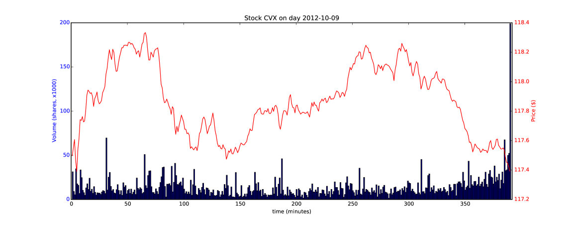
In other words we focus exclusively on the continuous trading activity without considering market opening and closing nor any over-the-counter trade. In Figure 1 we plot an example of market volumes and prices.

Figure 1: Example of a trading day. The blue bars are the market volumes traded every minute (in number of shares) and the red line is the period price $p_{t}$.

5.2 Market volumes model

We have so far assumed that the distribution of market volumes

$$f_{m}(m_{1},\ldots,m_{T})$$

is known from the start of the day. In reality a broker has a parametric family of distributions and each day (or less often) selects the parameters for the distribution with some statistical procedure. For simplicity, we assume such procedure is based on historical data. We found few works in the literature concerned with intraday market volumes modeling ([BDLF08]). We thus develop our own market volume model. This is composed of a parametric family of market volume distributions and an ad hoc procedure to choose the parameters with historical data.

For each stock we model the vector of market volumes as a multivariate log-normal. If the superscript $(k)$ refers to the stock $k$ (i.e., $m_{t}^{(k)}$ is the market volume for stock $k$ in interval $t$), we have

$$f_{m^{(k)}}(m^{(k)}_{1},\ldots,m^{(k)}_{T})\sim\ln\mathcal{N}(\mu+\mathbf{1}b^{(k)},\Sigma)$$ (34)

where $b^{(k)}\in{\mbox{\bf R}}$ is a constant that depends on the stock $k$ (each stock has a different typical daily volume), $\mu\in{\mbox{\bf R}}^{T}$ is an average “volume profile” (normalized so that $\mathbf{1}^{T}\mu=0$) and $\Sigma\in{\mbox{\bf S}}_{++}^{T}$ is a covariance matrix. The volume process thus separates into a per-stock deterministic component, modeled by the constant $b^{(k)}$, and a stochastic component with the same distribution for all stocks, modeled as a multivariate log-normal. We report in Appendix B the ad hoc procedure we use to estimate the parameters of this volume model on historical data and the formulas for the conditional expectations $\mathop{\bf E{}}_{t}\left[{1}/{V}\right]$, $\mathop{\bf E{}}_{t}[m_{\tau}]$, $\mathop{\bf E{}}_{t}\left[{1}/{m_{\tau}}\right]$ for $\tau=t,\ldots,T$ (which we need for the solution (33)). The procedure for estimating the volume model on past data requires us to provide a parameter, which we estimate with cross-validation on the initial section of the data. The details are explained in Appendix B.

5.3 Rolling testing

We organize our simulations according to a “rolling testing” or “moving window” procedure: for every day used to simulate order execution we estimate the various parameters on data from a “window” covering the preceding $W>0$ days. (It is commonly assumed that the most recent historical data are most relevant for model calibration since the systems underlying the observed phenomena change over time). We thus simulate execution on each day $i=W+1,\ldots,N$ using data from the days $i-W,\ldots,i-1$ for historical estimation.

In this way every time we test a VWAP solution algorithm, we use model parameters calibrated on historical data exclusively. In other words the performance of our models are estimated out-of-sample. In addition since all the order simulations use the same amount of historical data for calibration it is fair to compare them.

We fix the window lenght of the historical estimation to $W=20$, corresponding roughly to one month. We set aside the first $W_{CV}=10$ simulation days for cross-validating a feature of the volume model, as explained in Appendix B.2. In Figure 2 we describe the procedure. In the next two sections we explain how we perform the estimation of model parameters and simulation of orders execution.

Figure 2: Description of the rolling testing procedure. We iterate over the dataset, simulating execution on any day $i=W+1,\ldots,N$ and estimating the model parameters on the preceding $W=20$ days. The first $W_{CV}=10$ days used to simulate orders are reserved for cross validation (as explained in Appendix B.2). The aggregate results from the remaining $W+W_{CV}+1,\ldots,N$ days (30 days in total) are presented in §5.6.

5.4 Models estimation

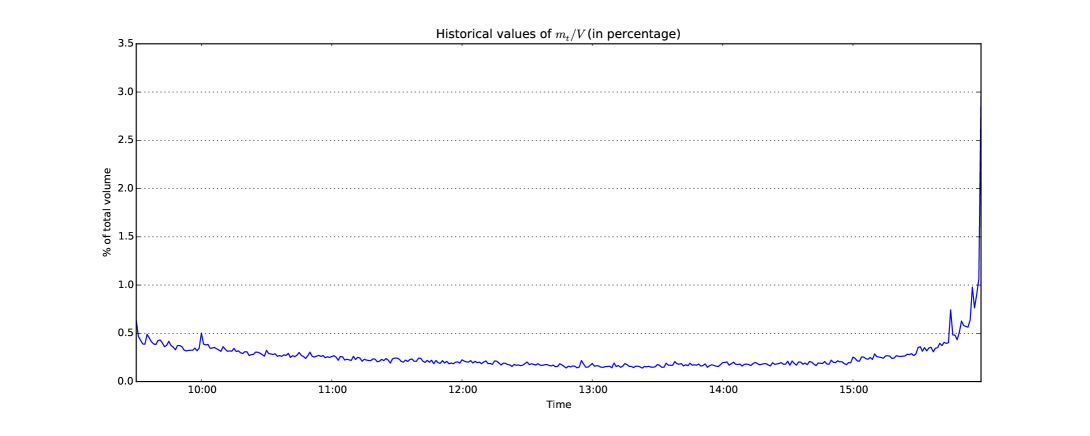
We describe the estimation, on historical data, of the parameters of all relevant models for our solution algorithms. We append the superscript $(i,k)$ to any quantity that refers to market day $i$ and stock $k$. We start by the market volumes per interval as a fraction of the total daily volume (which we need for (16)). We use the sample average

$$\mathop{\bf E{}}\left[\frac{m_{t}}{V}\right]\simeq\frac{\sum_{j=i-W}^{i-1}\sum_{k=1}^{K}{m_{t}^{(j,k)}}/{V^{(j,k)}}}{WK}$$

for every $t=1,\ldots,T$. An example of this estimation (on the first $W=20$ days of the dataset) is shown in Figure 3.

Figure 3: Estimated values of $\mathop{\bf E{}}\left[\frac{m_{t}}{V}\right]$ using the first $W=20$ days of our dataset, shown in percentage points.

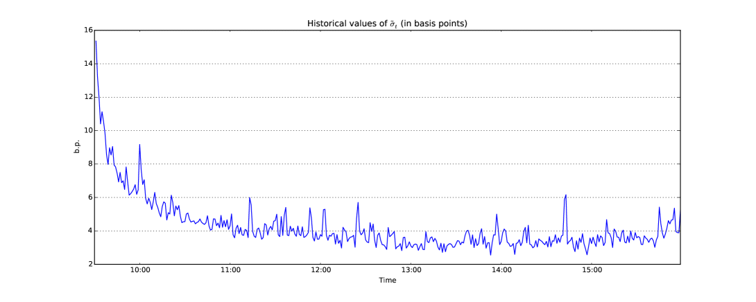
The dynamic solution (33) requires an estimate of the volatilites $\sigma_{t}$, we use the sample average of the squared price changes

$$\sigma_{t}^{2}\simeq\frac{\sum_{j=i-W}^{i-1}\sum_{k=1}^{K}{\left((p^{(j,k)}_{t+1}-p^{(j,k)}_{t})/p^{(j,k)}_{t}\right)}^{2}}{WK}$$

for every $t=1,\ldots,T$. In Figure 4 we show an example of this estimation (on the first $W$ days of the dataset).

Figure 4: Estimated values of the period volatilities, $\hat{\sigma}_{t}$ using the first $W=20$ days of our dataset. For each period of one minute these are the estimated standard deviation of the price increments, shown in basis points (one basis point is $0.0001$).

We then choose the volume distribution $f_{m}(m_{1},\ldots,m_{T})$ among the parametric family defined in §5.2 (using the ad hoc procedure described in Appendix B.1). We estimate the expected daily volume for each stock as the sample average

$$\mathop{\bf E{}}[V^{(i,k)}]\simeq\frac{\sum_{j=i-W}^{i-1}{V^{(j,k)}}}{W}$$

for every $k=1,\ldots,K$. We use this to choose the size of the simulated orders.

Finally, we consider the parameters $s_{1},\ldots,s_{T}$, and $\alpha$ of the transaction cost model (2). We do not estimate them empirically since we would need additional data, market quotes for the spread and proprietary data of executed orders for $\alpha$ (confidential for fiduciary reasons). We instead set them to exogenous values, kept constant across all stocks and days (to simplify comparison of execution costs). We assume for simplicity that the fractional spread is constant in time and equal to $2$ basis points, $s_{1}=\cdots=s_{T}=2\text{ b.p.}$ (one basis point is $0.0001$). That is reasonable for liquid stocks such as the ones from the DJIA. We choose the parameter $\alpha$ following a rule-of-thumb of transaction costs: trading one day’s volume costs approximately on day’s volatility [KGM03]. We estimate empirically over the first 20 days of the dataset the open-to-close volatility for our stocks, equal to approximately $90$ basis points, and thus from equation (2) we set $\alpha=90$.

5.5 Simulation of execution with VWAP solution algorithms

For each day $i=W+1,\ldots,N$ and each stock $k=1,\ldots,K$ we simulate the execution of a trading order. We fix the size of the order equal to $1\%$ of the expected daily volume for the given stock on the given day

$$C^{(i,k)}=\mathop{\bf E{}}[V^{(i,k)}]/100.$$

Such orders are small enough to have negligible impact on the price of the stock [BFL09], as we need for (2) to hold.

We repeat the simulation with different solution methods: the static solution (16) and the dynamic solution (33) with risk-aversion parameters $\lambda=0,1,10,100,1000,\infty$. We use the symbol $a$ to index the solution methods. For each simulation we solve the appropriate set of equations, setting all historically estimated parameters to the values obtained with the procedures of §5.4. For each solution method we obtain a simulated trading schedule

$$u_{t}^{(i,k,a)},\quad t=1,\ldots,T$$

where the superscript $a$ indexes the solution methods. We then compute the slippage incurred by the schedule using (4)

$$S^{(i,k,a)}=\frac{\sum_{t=1}^{T}p^{(i,k)}_{t}u_{t}^{(i,k,a)}-C^{(i,k)}p^{(i,k)}_{\text{VWAP}}}{C^{(i,k)}p^{(i,k)}_{\text{VWAP}}}+\sum_{t=1}^{T}\frac{s_{t}}{2}\left(\alpha\frac{{(u^{(i,k,a)}_{t})}^{2}}{C^{(i,k)}m^{(i,k)}_{t}}-\frac{u^{(i,k,a)}_{t}}{C^{(i,k)}}\right).$$ (35)

Note that we are simulating the transaction costs. Measuring them directly would require to actually execute $u_{t}^{(i,k,a)}$. This test of transaction costs optimization has value as a comparison between the static solution (16) and the dynamic solution (33). Our transaction costs model (2) is similar to the ones of other works in the literature (e.g., [FW13]) but involves the market volumes $m_{t}$. The static solution only uses the market volumes distribution known before the market opens, while the dynamic solution uses the SHDP procedure to incorporate real time information and improve modeling of market volumes. In the following we show that the dynamic solution achieves lower transaction costs than the static solution, such gains are due to the better handlng of information on market volumes.

In practice a broker would use a different model of transaction costs, perhaps more complicated than ours. We think that a good model should incorporate the market volumes $m_{t}$ as a key variable [BFL09]. Our test thus suggests that also in that setting the dynamic solution would perform better than the static solution.

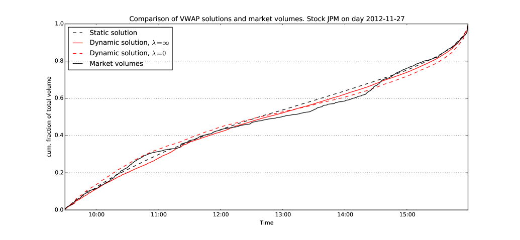
We show in Figure 5 the result of the simulation on a sample market day, using the static solution (16) and the dynamic solution (33) for $\lambda=0$ and $\infty$. We also plot the market volumes $m_{t}^{(i,k)}$.

Figure 5: Simulation of order execution on a sample market day. We report all volume processes as cumulative fraction of their total. At every time $\tau$ we plot $\sum_{t=1}^{\tau}\frac{m_{t}}{V}$ for the market volumes $m_{t}$ and $\sum_{t=1}^{\tau}\frac{u_{t}}{C}$ for the various solutions $u_{t}$. We only show the dynamic solution for $\lambda=0$ and $\lambda=\infty$ since for all other values of $\lambda$ the solution falls in between.

5.6 Aggregate results

We report the aggregate results from the simulation of VWAP execution on all the days reserved for orders simulation (minus the ones used for cross-validation). For any day $i=W+W_{CV}+1,\ldots,N$, stock $k=1,\ldots,K$, and solution method $a$ (either the static solution (16) or the dynamic solution (33) for various values of $\lambda$) we obtain the simulated slippage $S^{(i,k,a)}$ using (35). Then, for each solution method $a$ we define the empirical expected value of $S$ as

$$\mathop{\bf E{}}[S^{(a)}]=\frac{\sum_{i=W+W_{CV}+1}^{N}\sum_{k=1}^{K}S^{(i,k,a)}}{(N-W-W_{CV})K}$$

and the empirical variance

$$\mathop{\bf var}(S^{(a)})=\frac{\sum_{i=W+W_{CV}+1}^{N}\sum_{k=1}^{K}{(S^{(i,k,a)})}^{2}-\mathop{\bf E{}}[S^{(a)}]^{2}}{(N-W-W_{CV})K-1}.$$

In Figure 6 we show the values of these on a risk-reward plot. (We show the square root of the variance for simplicity, so that both axes are expressed in basis points).

Figure 6: Risk-reward plot of the aggregate results of our simulations on real market data. Each dot represents one solution method, either the static solution (16) or the dynamic solution (33) with risk-aversion parameters $\lambda=0,1,10,100,1000,\infty$. We show the sample average of the simulated slippages, which represents the execution costs, and the sample standard deviation, i.e., the root mean square error (RMSE) of tracking the VWAP. The orders have size equal to $1\%$ of the expected daily volume. The dynamic solution improves over the static solution in both dimensions, we can choose the preferred behaviour by fixing the risk-aversion parameter $\lambda$.

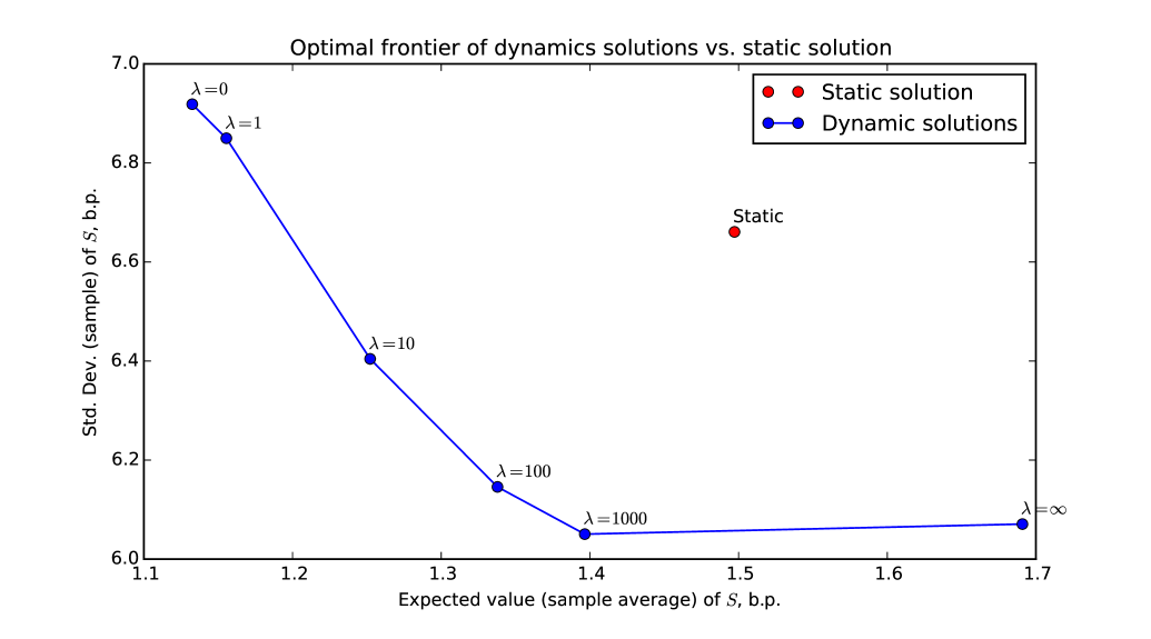
We observe that the dynamic solution improves over the static solution on both VWAP tracking (variance of $S$) and transaction costs (expected value of $S$), and we can select between the different behaviors by choosing different values of $\lambda$.

We introduced in §2.2 the approximation that the value of (10) is negligible when compared to (9). The empirical results validate this. For the static solution the empirical average value of (9) is $4.45e-07$ while (10) is $6.34e-09$, about $1\%$. For the dynamic solution with $\lambda=\infty$ the average value of (10) is $3.60e-07$ and (9) is $1.92e-08$, about $5\%$. For the dynamic solution with $\lambda=0$ instead the average value of (10) is $4.76e-07$ and (9) is $5.50e-09$, about $1\%$. The dynamic solutions for other values of $\lambda$ sit in between. Thus the approximation is generally valid, becoming less tight for high values of $\lambda$. In fact in Figure 6 we see that the empirical variance of $S$ for the dynamic solution with $\lambda=\infty$ is somewhat larger than the one with $\lambda=10000$, probably because of the contribution of (9). (We can interpret this as a bias-variance tradeoff since by going from $\lambda=\infty$ to $\lambda=10000$ we effectively introduce a regularization of the solution.)

6 Conclusions

We studied the problem of optimal execution under VWAP benchmark and developed two broad families of solutions.

The static solution of §3, although derived with similar assumptions to the classic [Kon02], is more flexible and can accommodate more sophisticated models (of bid-ask spread and volume) than the comparable static solutions in the literature. By formulating the problem as a quadratic program it is easy to add other convex constraints (see [MS12] for a good list) with a guaranteed straightforward fast solution [BV09].

The dynamic solution of §4 is the biggest contribution of this work. One one side, we manipulate the problem to fit it into the standard formalism of linear-quadratic stochastic control. On the other, we model the uncertainty on the total market volume (which is eschewed in all similar works we found in the literature) in a principled way, building on a recent result in optimal control [SBZ10].

The empirical tests of §5 are based on simulations with real data designed with good statistical practices (the rolling testing of §5.3 ensures that all results are obtained out-of-sample). We compare the performance of the static solution, standard in the trading industry, to our dynamic solution. The dynamic solution is built around a model for the joint distribution of market volumes, we provide a simple one in §5.2 (along with ad hoc procedures to use it). This is supposed to be a proof-of-concept since in practice a broker would have a more sophisticated market volume model, which would further improve performance of the dynamic solution. Even with our model for market volumes our dynamic solution improves the performance of the static solution significantly. The result validates all the approximations involved in the derivation of the dynamic solution and thus shows its value.

Our simulations quantify the improvements of our dynamic solution over the standard static solution. On one side we can reduce the RMSE of VWAP tracking by $10\%$. This is highly significant and could improve with a more sophisticated market volume model. On the other we can lower the execution costs by around $25\%$. In our test this corresponds to $\sim 50\$$ of savings for an order of a million dollars (the VWAP executions are worth billions of dollars each day).

Appendix A Dynamic programming equations

A.1 Riccati equations for LQSC

We derive the recursive formulas for (19) and (20). We know the final condition

$$v_{T+1}(x_{T+1})=g_{T+1}(x_{T+1}),$$

so $D_{T+1}=Q_{T+1}$, $d_{T+1}=d_{T+1}$, and $b_{T+1}=0$. Now for the inductive step, assume $v_{t+1}(x_{t+1})$ is in the form of (20) with known $D_{t+1}$, $d_{t+1}$, and $b_{t+1}$. Then the optimal action at time $t$ is, according to (18),

$$u_{t}=\mathop{\rm argmin}_{u}\mathop{\bf E{}}[g_{t}(x_{t},u,w_{t})+v_{t+1}(A_{t}(w_{t})x_{t}+B_{t}(w_{t})u+c_{t}(w_{t}))]=\\ K_{t}x_{t}+l_{t},$$

with

$$K_{t} = -\frac{\mathop{\bf E{}}[B_{t}(w_{t})^{T}D_{t+1}A_{t}(w_{t})]}{(\mathop{\bf E{}}R_{t}(w_{t})+\mathop{\bf E{}}[B_{t}(w_{t})^{T}D_{t+1}B_{t}(w_{t})]}$$

$$l_{t} = -\frac{\mathop{\bf E{}}r_{t}+2\mathop{\bf E{}}[B_{t}(w_{t})^{T}D_{t+1}c(w_{t})]+d_{t+1}^{T}\mathop{\bf E{}}B_{t}(w_{t})}{2(\mathop{\bf E{}}R_{t}(w_{t})+\mathop{\bf E{}}[B_{t}(w_{t})^{T}D_{t+1}B_{t}(w_{t})]}.$$

It follows that the value function at time $t$ is also in the form of (20), and it has value

$$v_{t}(x_{t})=\mathop{\bf E{}}\left[g_{t}(x_{t},K_{t}x_{t}+l_{t},w_{t})+v_{t+1}(A_{t}(w_{t})x_{t}+B_{t}(w_{t})(K_{t}x_{t}+l_{t})+c_{t}(w_{t}))\right]=\\ x_{t}^{T}D_{t}x_{t}+d_{t}^{T}x_{t}+b_{t}$$

with

$$D_{t} = \mathop{\bf E{}}Q_{t}(w_{t})+K_{t}^{T}\mathop{\bf E{}}\left[R_{t}(w_{t})+B_{t}(w_{t})^{T}D_{t+1}B_{t}(w_{t})\right]K_{t}+$$

$$\mathop{\bf E{}}[A_{t}(w_{t})^{T}D_{t+1}A_{t}(w_{t})]+K_{t}^{T}\mathop{\bf E{}}[B_{t}(w_{t})^{T}D_{t+1}A_{t}(w_{t})]+$$

$$\mathop{\bf E{}}[A_{t}(w_{t})^{T}D_{t+1}B_{t}(w_{t})]K_{t}$$

$$d_{t} = \mathop{\bf E{}}q_{t}(w_{t})+K^{T}_{t}\mathop{\bf E{}}r_{t}(w_{t})+2\mathop{\bf E{}}K^{T}_{t}R_{t}(w_{t})l_{t}+$$

$$\mathop{\bf E{}}[A_{t}(w_{t})+B_{t}(w_{t})K_{t})^{T}(d_{t+1}+2D_{t+1}(B_{t}(w_{t})l_{t}+\mathop{\bf E{}}c(w_{t}))]$$

$$b_{t} = b_{t+1}+\mathop{\bf E{}}R_{t}(w_{t})l_{t}^{2}+\mathop{\bf E{}}r_{t}(w_{t})l_{t}+$$

$$\mathop{\bf E{}}[(B_{t}(w_{t})l_{t}+c(w_{t}))^{T}D_{t+1}+d_{t+1}^{T})(B_{t}(w_{t})l_{t}+c(w_{t}))].$$

We thus completed the induction step, and so the value function is quadratic and the policy affine at every time step $t=1,\ldots,T$. The recursion can be solved as long as we know the functional form of the problem parameters and the distribution of the disturbances $w_{t}$.

A.2 SHDP Solution

We derive the recursive formulas for (31) and (32). These are equivalent to the Riccati equations we derived in Appendix A.1, but the expected values are taken over the marginal conditional densities $\hat{f}_{w_{\tau}|t}(\cdot)$. We write $\mathop{\bf E{}}_{t}$ to denote such expectation. In addition, these equations are somewhat simpler since our problem has $A_{t}(w_{t})=I$, $B_{t}(w_{t})=e_{1}$, $q_{t}=0$, and $r_{t}(w_{t})=r_{t}$ for $t=1,\ldots,T$. The final conditions are fixed by (29)

$$D_{T|t} = \mathop{\bf E{}}_{t}Q_{T}(w_{T})+e_{1}\mathop{\bf E{}}_{t}R_{T}(w_{T})e_{1}^{T}$$

$$d_{T|t} = -r_{T}e_{1}^{T}-2C\mathop{\bf E{}}_{t}R_{T}(w_{T})e_{1}^{T},$$

$$b_{T|t} = r_{T}C.$$

And the recursive equations are

$$K_{\tau|t} = -\frac{e_{1}^{T}D_{\tau+1|t}}{\mathop{\bf E{}}_{t}R_{\tau}(w_{\tau})+e_{1}^{T}D_{\tau+1}e_{1}}$$

$$l_{\tau|t} = -\frac{r_{\tau}+d_{\tau+1|t}^{T}e_{1}+2e_{1}^{T}D_{\tau+1|t}\mathop{\bf E{}}_{t}c(w_{\tau})}{2(\mathop{\bf E{}}_{t}R_{\tau}(w_{\tau})+e_{1}^{T}D_{\tau+1|t}e_{1})}$$

$$D_{\tau|t} = \mathop{\bf E{}}_{t}Q_{\tau}(w_{\tau})+K^{T}_{\tau|t}\left(\mathop{\bf E{}}_{t}[R_{\tau}(w_{\tau})]+e_{1}^{T}D_{\tau+1|t}e_{1}\right)K_{\tau|t}+$$

$$D_{\tau+1|t}+K_{\tau|t}^{T}e_{1}^{T}D_{\tau+1|t}+D_{\tau+1|t}e_{1}K_{\tau|t}=$$

$$\mathop{\bf E{}}_{t}Q_{\tau}(w_{\tau})+D_{\tau+1|t}+K_{\tau|t}^{T}e_{1}^{T}D_{\tau+1|t}$$

$$d_{\tau|t} = K_{\tau|t}^{T}r_{\tau}+2K_{\tau|t}^{T}\mathop{\bf E{}}_{t}R_{\tau}(w_{\tau})l_{\tau|t}+$$

$$(I+e_{1}K_{\tau|t})^{T}(d_{\tau+1|t}+2D_{\tau+1|t}(e_{1}l_{\tau|t}+\mathop{\bf E{}}_{t}c(w_{\tau})))=$$

$$d_{\tau+1|t}+2D_{\tau+1|t}(e_{1}l_{\tau|t}+\mathop{\bf E{}}_{t}c(w_{\tau}))$$

$$b_{\tau|t} = b_{\tau+1|t}+r_{\tau}l_{\tau|t}+\mathop{\bf E{}}_{t}R_{\tau}(w_{\tau})l_{\tau|t}^{2}+\mathop{\bf E{}}_{t}[c(w_{\tau})D_{\tau+1|t}c(w_{\tau})]+$$

$$d_{\tau+1|t}^{T}(e_{1}l_{\tau|t}+\mathop{\bf E{}}_{t}c(w_{\tau}))+l_{\tau|t}e_{1}^{T}D_{\tau+1|t}(e_{1}l_{\tau|t}+2\mathop{\bf E{}}_{t}c(w_{\tau}))=$$

$$b_{\tau+1|t}+\mathop{\bf E{}}_{t}[c(w_{\tau})D_{\tau+1|t}c(w_{\tau})]+d_{\tau+1|t}^{T}\mathop{\bf E{}}_{t}c(w_{\tau})$$

for $\tau=t,\ldots,T-1$.

A.3 SHDP simplied solution (without value function)

Parts of the equations derived in Appendix A.2 are superfluous in case we are not interested in the cost-to-go functions $v_{\tau|t}(x_{t})$ for $\tau=t,\ldots,T-1$. (In fact, we only want to compute the optimal action (33).) We disregard the constant term $b_{\tau|t}$, and we only compute the three scalar elements that we need from $D_{\tau|t}$ and $d_{\tau|t}$. For any $t=1,\ldots,T$ and $\tau=t,\ldots,T-1$ we define

$$e_{1}^{t}D_{\tau|t}e_{1} \equiv \beta_{\tau|t}$$

$$e_{1}^{t}D_{\tau|t}e_{2}=e_{2}^{t}D_{\tau|t}e_{1} \equiv \gamma_{\tau|t}$$

$$e_{1}^{t}d_{\tau|t} \equiv \delta_{\tau|t}$$

where $e_{1}=(1,0)$ and $e_{2}=(0,1)$ are the unit vectors. The final values are

$$\beta_{T|t} = \lambda\frac{\sigma_{T}^{2}}{C^{2}}+\frac{\alpha s_{T}}{2C}\mathop{\bf E{}}_{t}[{1}/{m_{T}}]$$

$$\gamma_{T|t} = -\lambda\frac{\sigma_{T}^{2}}{C}\mathop{\bf E{}}_{t}[1/V]$$

$$\delta_{T|t} = \frac{s_{T}}{2C}-{\alpha s_{T}}\mathop{\bf E{}}_{t}[{1}/{m_{T}}].$$

The policy

$$K_{\tau|t} = -\frac{(\beta_{\tau+1|t},\gamma_{\tau+1|t})}{({\alpha s_{\tau}}/{2C})\mathop{\bf E{}}_{t}[{1}/{m_{\tau}}]+\beta_{\tau+1|t}}$$

$$l_{\tau|t} = -\frac{-{s_{\tau}}/{(2C)}+\delta_{\tau+1|t}+2\gamma_{\tau+1|t}\mathop{\bf E{}}_{t}m_{\tau}}{2(({\alpha s_{\tau}}/{2C})\mathop{\bf E{}}_{t}[{1}/{m_{\tau}}]+\beta_{\tau+1|t})}.$$

We restrict the Riccati equations to these three scalars. They are independent from the rest of the recursion and we obtain

$$\beta_{\tau|t} = \lambda\frac{\sigma_{\tau}^{2}}{C^{2}}-\frac{\beta^{2}_{\tau+1|t}}{({\alpha s_{\tau}}/{2C})\mathop{\bf E{}}_{t}[{1}/{m_{\tau}}]+\beta_{\tau+1|t}}+\beta_{\tau+1|t}=$$

$$\lambda\frac{\sigma_{\tau}^{2}}{C^{2}}+\frac{({\alpha s_{\tau}}/{2C})\mathop{\bf E{}}_{t}[{1}/{m_{\tau}}]\beta_{\tau+1|t}}{({\alpha s_{\tau}}/{2C})\mathop{\bf E{}}_{t}[{1}/{m_{\tau}}]+\beta_{\tau+1|t}}$$

$$\gamma_{\tau|t} = -\lambda\frac{\sigma_{\tau}^{2}}{C}\mathop{\bf E{}}_{t}\left[1/{V}\right]-\frac{\beta_{\tau+1|t}\gamma_{\tau+1|t}}{({\alpha s_{\tau}}/{2C})\mathop{\bf E{}}_{t}[{1}/{m_{\tau}}]+\beta_{\tau+1|t}}+\gamma_{\tau+1|t}=$$

$$-\lambda\frac{\sigma_{\tau}^{2}}{C}\mathop{\bf E{}}_{t}\left[1/{V}\right]+\frac{({\alpha s_{\tau}}/{2C})\mathop{\bf E{}}_{t}[{1}/{m_{\tau}}]\gamma_{\tau+1|t}}{({\alpha s_{\tau}}/{2C})\mathop{\bf E{}}_{t}[{1}/{m_{\tau}}]+\beta_{\tau+1|t}}$$

$$\delta_{\tau|t} = \delta_{\tau+1|t}+2\beta_{\tau+1|t}l_{\tau|t}+2\gamma_{\tau+1|t}\mathop{\bf E{}}_{t}m_{t}.$$

A.3.1 Negligible spread

We study the case where $s_{t}=0$ for all $t=1,\ldots,T$, equivalent to the limit $\lambda\to\infty$. From the equations above we get that for all $t=1,\ldots,T$ and $\tau=t,\ldots,T$

$$\beta_{\tau|t} = \lambda\frac{\sigma_{\tau}^{2}}{C^{2}}$$

$$\gamma_{\tau|t} = -\lambda\frac{\sigma_{\tau}^{2}}{C}\mathop{\bf E{}}_{t}[1/V]$$

$$\delta_{\tau|t} = 0.$$

So for every $t=1,\dots,T$

$$\mu_{t|t}(x_{t})=K_{t|t}x_{t}+l_{t}=\frac{-(\beta_{\tau+1|t},\gamma_{\tau+1|t})x_{t}-\mathop{\bf E{}}_{t}m_{t}\gamma_{\tau+1|t}}{\beta_{t+1|t}}=\\ C\mathop{\bf E{}}_{t}\left[1/{V}\right]\left(\sum_{\tau=1}^{t-1}m_{\tau}+\mathop{\bf E{}}_{t}m_{t}\right)-\sum_{\tau=1}^{t-1}u_{\tau}.$$

In other words, at every point in time we look at the difference between the fraction of order volume we have executed and the fraction of daily volume the market has traded (using our most recent estimate of the total volume). We trade the expected fraction for next period $C\mathop{\bf E{}}_{t}\left[1/{V}\right]\mathop{\bf E{}}_{t}m_{t}$, plus this difference.

Appendix B Volume model

We explain here the details of the volume model (34), which we use for the dynamic VWAP solution. In §B.1 we describe the ad hoc procedure we use to estimate the parameters of the model on historical data. Then in §B.2 we detail the cross-validation of a particular feature of the model. Finally in §B.3 we derive formulas for the expected values of some functions of the volume, which we need for the solution (33).

B.1 Estimation on historical data

We consider estimation of the volume model parameters $b^{(k)}$, $\mu$ and $\Sigma$ using data from days $i-W,\ldots,i-1$ (we are solving the problem at day $i$). We append the superscript $(i,k)$ to any quantity that refers to market day $i$ and stock $k$.

Estimation of $b^{k}$

We first estimate the value of $b^{(k)}$ for each stock $k$, as:

$$\hat{b}^{(k)}=\frac{\sum_{j=i-W}^{i-1}\sum_{t=1}^{T}\log m_{t}^{(j,k)}}{TW}$$

We show in Table 1 the values of $\hat{b}^{(k)}$ obtained on the first $W$ days of our dataset.

Stock	$\hat{b}^{(k)}$	Stock	$\hat{b}^{(k)}$
AA	4.338	JPM	4.599
AXP	3.910	KO	4.312
BA	3.845	MCD	4.017
BAC	5.309	MMM	3.701
CAT	4.118	MRK	4.176
CSCO	4.693	MSFT	4.848
CVX	3.986	PFE	4.586
DD	3.990	PG	4.088
DIS	4.055	T	4.566
GE	4.784	TRV	3.546
HD	4.139	UNH	3.902
HPQ	4.577	UTX	3.782
IBM	3.788	VZ	4.225
INTC	4.860	WMT	3.992
JNJ	4.244	XOM	4.260

Table 1: Empirical estimate $\hat{b}^{(k)}$ of the per-stock component of the volume model, using data from the first $W=20$ days.

Estimation of $\mu$

Since each observation $\log m^{(j,k)}-\mathbf{1}b^{(j,k)}$ is distributed as a multivariate Gaussian we use this empirical mean as estimator of $\mu$:

$$\hat{\mu}_{t}=\frac{\sum_{j=i-W}^{i-1}\sum_{k=1}^{K}\log m^{(j,k)}_{t}-\hat{b}^{(k)}}{WK}.$$

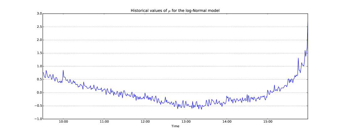
We plot in Figure (7) the value of $\hat{\mu}$ obtained on the first $W$ days of our dataset.

Figure 7: Empirical estimate $\hat{\mu}$ of the cross-time component of the volume model, using data from the first $W=20$ days.

Estimation of $\Sigma$

We finally turn to the estimation of the covariance matrix $\Sigma\in{\mbox{\bf S}}^{T}_{++}$, using historical data. In general, empirical estimation of covariance matrices is a complicated problem. Typically one has not access to enough data to avoid overfitting (a covariance matrix has $O(N^{2})$ degrees of freedom, where $N$ is the dimension of a sample). Many approximate approaches have been developed in the econometrics and statistics literature. We designed an ad hoc procedure, inspired by works such as [FLM11]. We look for a matrix of the form

$$\Sigma=ff^{T}+S,$$

where $f\in{\mbox{\bf R}}^{T}$ and $S\in{\mbox{\bf S}}^{T}_{++}$ is sparse. We first build the empirical covariance matrix. Let $X\in{\mbox{\bf R}}^{T\times{(WK)}}$ be the matrix whose columns are vectors of the form:

$$\log m^{(j,k)}-\mathbf{1}\hat{b}^{(k)}-\hat{\mu}$$

for each day $j=i-W,\ldots,i-1$ and stock $k=1,\ldots,K$. Then the empirical covariance matrix is

$$\hat{\Sigma}=\frac{1}{WK-1}XX^{T}.$$

We perform the singular value decomposition of $X$

$$X=U\cdot\mathop{\bf diag}({s_{1},s_{2},\ldots,s_{T}})\cdot V^{T},$$

where $s\in{\mbox{\bf R}}^{T}$, $s_{1}\geq s_{2}\geq...\geq s_{T}\geq 0$, $U\in{\mbox{\bf R}}^{T\times T}$, and $V\in{\mbox{\bf R}}^{(WK)\times T}$ (because in practice we have $WK>T$, since $W=20$, $K=30$, and $T=390$). We have

$$\hat{\Sigma}=\frac{1}{WK-1}U\cdot\mathop{\bf diag}(s_{1}^{2},s_{2}^{2},\ldots,s^{2}_{T})\cdot U^{T}.$$

We show in Figure 8 the first singular values $s_{1},s_{2},\ldots,s_{20}$ computed on data from the first $W$ days.

Figure 8: First 20 singular values of the matrix $X$ of observations $\log m^{(j,k)}-\mathbf{1}\hat{b}^{(k)}-\hat{\mu}$.

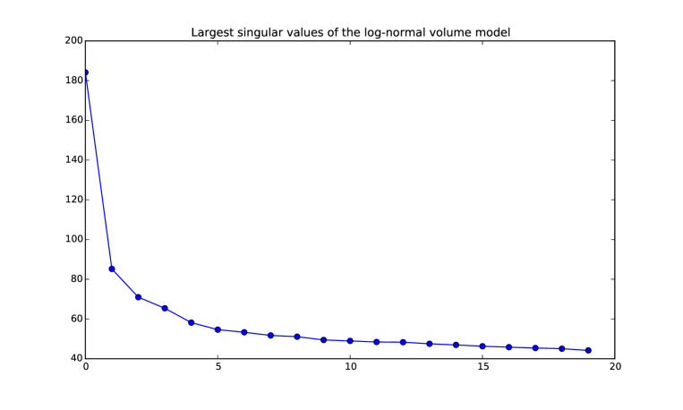
It is clear that the first singular value is much larger than all the others. We thus build the rank 1 approximation of the empirical covariance matrix by keeping the first singular value and first (left) singular vector

$$f=\frac{s_{1}U_{:,1}}{\sqrt{WK-1}},$$

so that $ff^{T}$ is the best (in Frobenius norm) rank-1 approximation of $\hat{\Sigma}$. We now need to provide an approximation for the sparse part $S$ of the covariance matrix. We assume that $S$ is a banded matrix of bandwidth $b>0$, which is non-zero only on the main diagonal and on $b-1$ diagonals above and below it (in total it has $2b-1$ non-zero diagonals). The value of $b$ is chosen by cross-validation, as explained in §B.2. The assumption that $S$ is banded is inspired by the intuition that elements of $\log m^{(j,k)}-\mathbf{1}b^{(k)}-\mu$ are correlated (in time) for short delays. We find $S$ by simply copying the diagonal elements of the empirical covariance matrix:

$$\cdot S_{i,j}=\begin{cases}(\hat{\Sigma}-ff^{T})_{i,j}&\mbox{ if }|j-i|\leq b\\ 0&\mbox{ otherwise. }\\ \end{cases}$$

We thus have built a matrix of the form ${\Sigma}=ff^{T}+S.$ Note that this procedure does not guarantee that ${\Sigma}$ is positive definite. However in our empirical tests we always got positive definite ${\Sigma}$ for any $b=1,2,\ldots$.

B.2 Cross validation

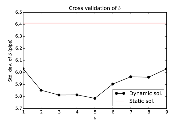
As explained in §B.1, we need to choose the value of the parameter $b\in\mathbb{N}$ (used for empirical estimation of the covariance matrix $\Sigma$). We choose it by cross-validation, reserving the first $W_{CV}=10$ testing days of the dataset. We show in Figure 2 the way we partition the data (so that the empirical testing is performed out-of-sample with respect to the cross-validation). We simulate trading according to the solution (33) with $\lambda=\infty$ (i.e., the special case of Appendix A.3.1), for various values of $b$. We then compute the empirical variance of $S$, and choose the value of $b$ which minimizes it. (We are mostly interested in optimizing the variance of $S$, rather than the transaction costs.) In Figure 9 we show the result of this procedure (we show the standard deviations instead of variances, for simplicity), along with the result using the static solution (16), for comparison. Since the difference in performance between $b=3$ and $b=5$ is small (and we want to avoid overfitting), we choose $b=3$.

Figure 9: To cross validate the volume model parameter $b$, we compute the empirical standard deviation of $S$ for the dynamic solution (33) with $\lambda=\infty$, changing the value of $b$ in the volume model. We also show the static solution (16), which does not use the volume model, for comparison. From this result we choose $b=3$ (to avoid overfitting).

B.3 Expected values of interest

We consider the problem at any fixed time $t=1,\ldots,T-1$, for a given stock $k$ and day $i$. (We have observed market volumes $m_{1},\ldots,m_{t-1}$.) We obtain the conditional distribution of the unobserved volumes $m_{t},\ldots,m_{T}$ and derive expressions for $\mathop{\bf E{}}_{t}m_{\tau}$, $\mathop{\bf E{}}_{t}\left[\frac{1}{m_{\tau}}\right]$, and $\mathop{\bf E{}}_{t}\left[\frac{1}{V}\right]$ for any $\tau=t,\ldots,T$. We need these for the numerical solution (33), as developed in Appendix A.3.1.

Conditional distribution

We divide the covariance matrix in blocks:

$$\Sigma=\left(\begin{array}[]{cc}\Sigma_{1:(t-1),1:(t-1)}&\Sigma_{1:(t-1),t:T}\\ \Sigma_{t:T,1:(t-1)}&\Sigma_{t:T,t:T}\end{array}\right).$$

Then we get the marginal distribution

$$m_{t:T}\sim\log\mathcal{N}(\nu{|{t}},\Sigma{|{t}})$$

by taking the Schur complement (e.g., [BV09]) of the covariance matrix

$$\nu{|{t}} \equiv \mu_{{t}:T}+b^{(k)}+\Sigma_{1:(t-1),t:T}^{T}\Sigma_{1:(t-1),1:(t-1)}^{-1}(\log m_{1:({t}-1)}-\mu_{1:({t}-1)}-b^{(k)})$$

$$\Sigma{|{t}} \equiv \Sigma_{t:T,t:T}-\Sigma_{1:(t-1),t:T}^{T}\Sigma_{1:(t-1),1:(t-1)}^{-1}\Sigma_{1:(t-1),t:T}.$$

Note that $\nu{|1}=\mu+b^{(k)}$ and $\Sigma{|1}=\Sigma$, i.e., the unconditional distribution of the market volumes. We now develop the conditional expectation expressions.

Volumes

The expected value of the remaining volumes $m_{\tau}$

$$\mathop{\bf E{}}_{t}m_{\tau}=\exp\left((\nu{|t})_{\tau-t+1}+\frac{(\Sigma|t)_{\tau-t+1,\tau-t+1}}{2}\right),\quad\tau=t,\ldots,T.$$

(Because the $(\tau-t+1)$-th element of $\nu{|t}$ corresponds to the $\tau$-th volume.)

Inverse volumes

The expected value of the inverse of the remaining volumes $m_{\tau}$

$$\mathop{\bf E{}}_{t}\left[\frac{1}{m_{\tau}}\right]=\exp\left({-(\nu{|t})_{\tau-t+1}+\frac{(\Sigma|t)_{\tau-t+1,\tau-t+1}}{2}}\right),\quad\tau=t,\ldots,T.$$

Total volume

We have, since we already observed $m_{1},\ldots,m_{t-1}$

$$\mathop{\bf E{}}_{t}V=\sum_{\tau=1}^{t-1}m_{\tau}+\sum_{\tau=t}^{T}\mathop{\bf E{}}_{t}m_{\tau}.$$

We also express its variance, which we need later

$$\mathop{\bf var}_{t}(V)=\mathop{\bf var}_{t}\sum_{\tau=t}^{T}m_{\tau}=\sum_{\tau=t}^{T}\sum_{\tau^{\prime}=t}^{T}\mathbf{cov}(m_{\tau},m_{\tau^{\prime}})=\\ \sum_{\tau=t}^{T}\sum_{\tau^{\prime}=t}^{T}\mathop{\bf E{}}_{t}m_{\tau}\mathop{\bf E{}}_{t}m_{\tau^{\prime}}\left(\exp((\Sigma|t)_{\tau-t+1,\tau^{\prime}-t+1})-1\right).$$

Inverse total volume

We use the following approximation, derived from the Taylor expansion formula. Consider a random variable $z$ and a smooth function $\phi(\cdot)$, then

$$\mathop{\bf E{}}\phi(z)\simeq\phi(\mathop{\bf E{}}z)+\frac{\phi^{\prime\prime}(\mathop{\bf E{}}z)}{2}\mathop{\bf var}z.$$

So the inverse total volume

$$\mathop{\bf E{}}_{t}\left[\frac{1}{V}\right]\simeq\frac{1}{\mathop{\bf E{}}_{t}{V}}+\frac{\mathop{\bf var}_{t}(V)}{\mathop{\bf E{}}_{t}[{V}]^{3}}.$$

References

- [AC01] Robert Almgren and Neil Chriss. Optimal execution of portfolio transactions. Journal of Risk, 3:5–40, 2001.
- [BDLF08] Jedrzej Białkowski, Serge Darolles, and Gaëlle Le Fol. Improving vwap strategies: A dynamic volume approach. Journal of Banking & Finance, 32(9):1709–1722, 2008.
- [Bem06] Alberto Bemporad. Model predictive control design: New trends and tools. In Decision and Control, 2006 45th IEEE Conference on, pages 6678–6683. IEEE, 2006.
- [Ber95] Dimitri P Bertsekas. Dynamic programming and optimal control, volume 1. Athena Scientific Belmont, MA, 1995.
- [BFL09] J.P. Bouchaud, J.D. Farmer, and F. Lillo. How markets slowly digest changes in supply and demand, volume 4 of Handbook of financial markets. North-Holland, San Diego, CA, 2009.
- [BL98] Dimitris Bertsimas and Andrew W Lo. Optimal control of execution costs. Journal of Financial Markets, 1(1):1–50, 1998.
- [BLR12] Stephen Boyd, Sanjay Lall, and Ben Van Roy. Ee365: Stochastic control. http://stanford.edu/class/ee365/lectures.html, 2012.
- [BMOW13] Stephen Boyd, Mark Mueller, Brendan ODonoghue, and Yang Wang. Performance bounds and suboptimal policies for multi-period investment. Foundations and Trends in Optimization, 1(1):1–69, 2013.
- [BV09] Stephen Boyd and Lieven Vandenberghe. Convex optimization. Cambridge university press, 2009.
- [DCB13] Alexander Domahidi, Eric Chu, and Stephen Boyd. Ecos: An socp solver for embedded systems. In Control Conference (ECC), 2013 European, pages 3071–3076. IEEE, 2013.
- [DCB14] Steven Diamond, Eric Chu, and Stephen Boyd. CVXPY: A Python-embedded modeling language for convex optimization, version 0.2. http://cvxpy.org/, May 2014.
- [FLM11] Jianqing Fan, Yuan Liao, and Martina Mincheva. High dimensional covariance matrix estimation in approximate factor models. Annals of statistics, 39(6):3320, 2011.
- [FW13] Christoph Frei and Nicholas Westray. Optimal execution of a vwap order: a stochastic control approach. Mathematical Finance, 2013.
- [GB14] Michael Grant and Stephen Boyd. CVX: Matlab software for disciplined convex programming, version 2.1. http://cvxr.com/cvx, March 2014.
- [GR13] Olivier Guéant and Guillaume Royer. Vwap execution and guaranteed vwap. arXiv preprint arXiv:1306.2832, 2013.
- [HJ11] Mark L Humphery-Jenner. Optimal vwap trading under noisy conditions. Journal of Banking & Finance, 35(9):2319–2329, 2011.
- [KB14] Arezou Keshavarz and Stephen Boyd. Quadratic approximate dynamic programming for input-affine systems. International Journal of Robust and Nonlinear Control, 24(3):432–449, 2014.
- [KGM03] R. Kissell, M. Glantz, and R. Malamut. Optimal Trading Strategies: Quantitative Approaches for Managing Market Impact and Trading Risk. AMACOM, New York, NY, 2003.
- [KH06] Wook Hyun Kwon and Soo Hee Han. Receding horizon control: model predictive control for state models. Springer Science & Business Media, 2006.
- [Kon02] Hizuru Konishi. Optimal slice of a vwap trade. Journal of Financial Markets, 5(2):197–221, 2002.
- [LFM03] F. Lillo, J.D. Farmer, and R.N. Mantegna. Master curve for price-impact function. Nature, 421(129):176–190, 2003.
- [Li13] Tianhui Michael Li. Dynamic Programming and Trade Execution. PhD thesis, PRINCETON UNIVERSITY, 2013.
- [Mad02] Ananth N Madhavan. Vwap strategies. Trading, 2002(1):32–39, 2002.
- [MK12] James McCulloch and Vlad Kazakov. Mean variance optimal vwap trading. Available at SSRN 1803858, 2012.
- [MS12] Ciamac C Moallemi and Mehmet Saglam. Dynamic portfolio choice with linear rebalancing rules. Available at SSRN 2011605, 2012.
- [MWB11] Jacob Mattingley, Yang Wang, and Stephen Boyd. Receding horizon control. Control Systems, IEEE, 31(3):52–65, 2011.
- [OW05] Anna Obizhaeva and Jiang Wang. Optimal trading strategy and supply/demand dynamics. NBER Working Papers, http://ideas.repec.org/p/nbr/nberwo/11444.html 11444, National Bureau of Economic Research, June 2005.
- [Pow07] Warren B Powell. Approximate Dynamic Programming: Solving the curses of dimensionality, volume 703. John Wiley & Sons, 2007.
- [SBZ10] Joëlle Skaf, Stephen Boyd, and Assaf Zeevi. Shrinking-horizon dynamic programming. International Journal of Robust and Nonlinear Control, 20(17):1993–2002, 2010.
- [TAQ] Wharton Research Data Services, TAQ Dataset. https://wrds-web.wharton.upenn.edu/wrds/.