Limiting SUSY compressed spectra scenarios

Abstract

Typical searches for supersymmetry cannot test models in which the two lightest particles have a small (“compressed”) mass splitting, due to the small momentum of the particles produced in the decay of the second-to-lightest particle. However, datasets with large missing transverse momentum ($E_{\rm T}^{\rm miss}$) can generically search for invisible particle production and therefore provide constraints on such models. We apply data from the ATLAS mono-jet (jet+$E_{\rm T}^{\rm miss}$) and vector-boson-fusion (forward jets and $E_{\rm T}^{\rm miss}$) searches to such models. The two datasets have complementary sensitivity, but in all cases experimental limits are at least five times weaker than theoretical predictions.

I Introduction

Models of supersymmetry (SUSY) remain leading candidates for new physics despite increasingly stringent constraints from collider searches. In particular, the lightest SUSY particle (LSP, also denoted as $\chi^{0}_{1}$) is a prototypical candidate for ‘weakly interacting massive particle’ (WIMP) dark matter. Conventional searches for SUSY require that the mass splitting between the invisible LSP and the next-to-lightest SUSY particle is large enough to produce a visible probe, such as a charged lepton. However, many interesting SUSY models have a splitting which is very small, known as compressed spectra, to which these limits do not apply.

In the minimal supersymmetric Standard Model (MSSM), the neutralino is an admixture of the neutral Higgsinos and gauginos. To obtain a realistic dark matter candidate, one must typically balance the large annihilation rates of the Higgsinos ($\tilde{h}_{u,d}$) or SU(2) gauginos (winos) against the small annihilation rates of the hypercharge gaugino (the bino, $\tilde{B}$) to yield the correct dark matter relic abundance through thermal freeze-out; this tuning of admixtures is called a ‘well-tempered neutralino’ Arkani-Hamed et al. (2006). This scenario is naturally associated with a compressed spectrum. In the case of a bino–Higgsino LSP, the tuning of the $\tilde{B}$ and $\tilde{h}_{u,d}$ masses typically gives a splitting between the LSP and the next-lightest states of $\mathcal{O}(M_{Z})$.

In this paper, we probe this experimentally challenging yet theoretically important region using two broadly powerful datasets from the ATLAS experiment: the “mono-jet”Aad et al. (2015a) final state (one or more jets with large missing transverse momentum) and the dataset used to search for vector-boson-fusion (VBF) production of a Higgs boson Aad et al. (2015b) which decays invisibly (two forward jets and large missing transverse momentum). Previously, analyses have applied the mono-jet limits to compressed spectra scenarios with electroweakinos Schwaller and Zurita (2014); Han et al. (2014, 2015), phenomenological MSSM Aad et al. (2015c), or simplified models of the MSSM Arbey et al. (2015); or calculated projected LHC sensitivity to VBF scenarios Giudice et al. (2010); Dutta et al. (2013); Delannoy et al. (2013a). To our knowlegde, this is the first application of the VBF dataset to these SUSY scenarios.

These data are applied to evaluate the constraints on supersymmetric models with compressed spectra in which all supersymmetric partners except the electroweak gauginos are very massive Arkani-Hamed et al. (2006); Giudice et al. (2010); Delannoy et al. (2013b). We do not impose that the thermal relic abundance of the LSP matches that of dark matter and allow the possibility of non-thermal production or multi-component dark matter Gelmini and Gondolo (2010); Cheung et al. (2013). Direct detection bounds are discussed in Cheung et al. (2013), where it is also noted that the well-tempering region considered in this work below overlaps with a blind spot in spin-independent direct detection constraints.

II Theory

We review the main features of bino–Higgsino dark matter in the well-tempered, blind-spot limit following the discussions in Arkani-Hamed et al. (2006) and Cheung et al. (2013). This is a region of the Minimal Supersymmetric Standard Model where we take the limit where the gluino and the scalar superpartners of Standard Model fermions are decoupled so that (1) they play no role in the dynamics of the dark matter and (2) the models are not excluded by colored sparticle searches from Run I. We shall further take the case where the SU(2) gaugino mass and CP-odd Higgs mass are taken very large compared to the other electroweak fermionic sparticle mass parameters, $M_{2},M_{A}\gg M_{1},|\mu|$ so that the winos and additional Higgses decouple. We are left with a theory that extends the Standard Model with two charged fermions $\chi_{1}^{\pm}$ of mass $M_{\chi_{1}^{\pm}}\approx|\mu|$ and three neutral fermion states, $\tilde{B}$, $\tilde{h}_{u,d}$ which mix into three mass eigenstates $\chi^{0}_{1,2,3}$, the lightest of which is identified with dark matter Feng et al. (2000, 2001); Baer et al. (2002); Giudice and Romanino (2004); Pierce (2004); Masiero et al. (2005); Arkani-Hamed et al. (2006); Baer et al. (2007). The parameters of this theory are assumed real and are the bino mass, $M_{1}>0$, the Higgsino mass, $\mu$ (taking either sign), and the ratio of the Higgs vacuum expectation values, $\tan\beta$. We further assume $M_{1},|\mu|>M_{Z}$.

II.1 Well Tempering and Compressing

The well-tempering condition in the bino–Higgsino theory described above is that $M_{1}\approx|\mu|$. It is useful to go to an intermediate basis of states,

$$\tilde{B} \tilde{h}_{-}\equiv\frac{\tilde{h}_{u}-\tilde{h}_{d}}{\sqrt{2}} \tilde{h}_{+}\equiv\frac{\tilde{h}_{u}+\tilde{h}_{d}}{\sqrt{2}}.$$ (1)

In this basis, the neutralino mass matrix is

$$\begin{pmatrix}M_{1}&-\frac{s_{\beta}+c_{\beta}}{\sqrt{2}}s_{W}M_{Z}&\frac{c_{\beta}-s_{\beta}}{\sqrt{2}}s_{W}M_{Z}\\ -\frac{s_{\beta}+c_{\beta}}{\sqrt{2}}s_{W}M_{Z}&\mu&0\\ \frac{s_{\beta}-c_{\beta}}{\sqrt{2}}s_{W}M_{Z}&0&-\mu\end{pmatrix}$$ (2)

up to higher order terms suppressed by $M_{W}^{2}/M_{2}\ll M_{Z}$ and where $s_{\beta}$ and $c_{\beta}$ are $\sin\beta$ and $\cos\beta$ respectively.

We are interested in the regime where the spectrum is compressed,

$$\left|M_{1}\pm\mu\right|<\frac{s_{\beta}\mp c_{\beta}}{\sqrt{2}}s_{W}M_{Z}$$ (3)

for $M_{1}\approx\mp\mu$. In this case, a pair of diagonal elements are nearly degenerate relative to their off-diagonal elements and and this $2\times 2$ block is maximally mixed giving an approximate spectrum

$$M_{\chi^{0}_{1}} \approx M_{1}-\frac{s_{\beta}\pm c_{\beta}}{\sqrt{2}}s_{W}M_{Z}+\mathcal{O}\left(\frac{M_{Z}^{2}}{M_{1}}\right)$$ (4)

$$M_{\chi^{0}_{2}} \approx M_{1}+\mathcal{O}\left(\frac{M_{Z}^{2}}{M_{1}}\right)$$ (5)

$$M_{\chi^{0}_{3}} \approx M_{1}+\frac{s_{\beta}\pm c_{\beta}}{\sqrt{2}}s_{W}M_{Z}+\mathcal{O}\left(\frac{M_{Z}^{2}}{M_{1}}\right).$$ (6)

This gives an LSP which is $\tilde{B}$–$\tilde{h}_{+}$ ($\tilde{B}$–$\tilde{h}_{-}$) for the case $\mu<0$ ($\mu>0$).

For the case $\mu<0$, observe that that as $\tan\beta\to 1$, (3) fails and the diagonal elements are split by more than the off-diagonal elements. In this case the mixing remains small and the mass eigenstates are dominantly those in (1). This may cause concern that the well-tempering is no longer effective since the LSP is no longer well-mixed between the ‘too small annihilation rate’ bino and the ‘too large annihilation rate’ Higgsinos. This is not the case, since even in the well-mixed case, the correct LSP relic abundance is obtained through coannihilation with the other neutralinos and charginos which are very close in mass to the LSP Griest and Seckel (1991). In other words, the well-tempering for the LSP relic abundance and compressed spectra go hand-in-hand.

II.2 Blind Spotting

Thus far $\tan\beta$ has been a free parameter that controls the relative mixing of the bino with the different Higgsinos in (6). It was pointed out in Cheung et al. (2013) that $\tan\beta$ controls slices of parameter space where the direct detection experiments are blind to the LSP. The LSP–Higgs coupling is uniquely responsible for spin-independent direct detection since Majorana particles like the neutralinos have no vector current. We consider a slice of parameter space where this LSP–Higgs coupling vanishes, focusing specifically on the case where

$$M_{1}+\mu\sin 2\beta=0.$$ (7)

The vanishing of the LSP coupling to the Higgs is simple to see heuristically: in this case $\mu<0$ so that the LSP is a $\tilde{B}$–$\tilde{h}_{+}$ mixture, following the analysis above. The relevant coupling to the Higgs comes from the $\tilde{B}\tilde{h}_{u,d}h_{u,d}$ gauge interactions. Thus the LSP–Higgs coupling comes from $\tilde{B}(\tilde{h}_{u}+\tilde{h}_{d})h$ and is diagrammatically

(8)

where $c_{u}$ and $c_{d}$ are the bino–Higgsino–Higgs gauge couplings for the up- and down-type neutral Higgsinos respectively. Recalling that the up-type and down-type Higgs supermultiplets have opposite hypercharge, $c_{u}=-c_{d}$ so that the LSP–Higgs coupling vanishes. Taking the full mixing into account, the position of the blind spot is controlled by $\tan\beta$ through the $\sin 2\beta$ in (7).

In the case where $\tan\beta\to 1$, $\sin 2\beta\to 1$ and (7) is compatible with to the well-tempered condition $M_{1}\approx|\mu|$. Indeed, this also aligns with a blind spot for spin-dependent direct detection since in this limit, left-right parity is restored between the $\tilde{h}_{u,d}$ so that the parity-violating spin-dependent cross section vanishes.

II.3 Sketched Phenomenology

We thus consider the scenario where $\mu\to-M_{1}$ and $\tan\beta\to 1$ in which we live in a double-blind spot against spin-independent and spin-dependent direct detection experiments. As remarked above, there is a qualitative difference depending on which condition is more closely met: either the LSP is very well mixed between $\tilde{B}$ and $\tilde{h}_{+}$ or it is a pure $\tilde{h}_{+}$ state, depending on which of $M_{1}$ or $|\mu|$ is smaller. As noted, this has a small effect on the relic abundance since this is well-tempered through coannihilations with the nearly-degenerate states. This also affects the specific couplings of the electroweakinos at colliders, though we do not expect this to affect the searches we present here. The smallness of $\tan\beta$ (combined with the decoupling of scalar superpartners) also avoids the most stringent bounds flavor-changing neutral currents such as $B_{s}\to\mu\mu$ Gogoladze et al. (2011).

We remark that it there is conventional wisdom that LEP excludes the MSSM with $\tan\beta\lesssim\mathcal{O}(\text{few})$ so that one may question the $\tan\beta\to 1$ limit taken here. This statement, however, depends on the conventional assumption that the scale of the scalar superpartners of the Standard Model fermions, $M_{S}$, is close to the TeV scale. This assumption is tied to the naturalness of the MSSM. In the absence of new physics, it is perhaps useful to relax any bias about the form of naturalness and instead search more broadly. This approach has recently been advocated in Djouadi et al. (2015, 2013); Djouadi and Quevillon (2013) where it is pointed out that the low-$\tan\beta$ regime re-opens for decoupled scalar superparters—the limit we take here. The $\tan\beta\sim$ few limit is qualitatively similar and relaxes the lower limit on $M_{S}$.

We do not perform a detailed phenomenological study of this slice of the MSSM, such as checking precise values of the relic abundance or bounds from indirect detection, and leave this to future work. See Cheung et al. (2013) for a detailed study and parameter scan which validates the existence of phenomenologically viable models along this region. We focus on the specific slice $\mu=-M_{1}$ and $\tan\beta=1$, noting that theories that are nearby behave qualitatively the same. We also present results for $\tan\beta=15$ as a benchmark for how the model behaves for more moderate $\tan\beta$ values. See, for example Masiero et al. (2005); Bernal et al. (2007) for further phenomenological considerations as one deviates from the doubly-blind spot, and Cahill-Rowley et al. (2015) for a more general status report in the phenomenological MSSM.

Finally, we note we treat the MSSM as a framework for models that populate this bino–Higgsino regime that are themselves UV complete but also span a range of phenomenology that is applicable to a broad range of models beyond the MSSM. An alternative approach is to consider minimal simplified models that can populate the analogous phenomenology, such as singlet–doublet models Cohen et al. (2012). In the remainder of this document, we explore the ability of collider searches to expose this difficult-to-probe region of the bino–Higgsino parameter space despite its compressed spectra.

III Signal generation

The parameters $M_{1}$, $M_{2}$, $\mu$ and $\tan\beta$ control the mixings, couplings, and masses of the gauginos. These parameters are generated along a line

$$M_{1}=-\mu,$$ (9)

with $\tan\beta=$ 1 and 15 and decoupled wino, $M_{2}=4000~{}\text{GeV}\gg M_{1}$. This gives a well-tempered bino-Higgsino LSP. Multi-jet final states produced in association with two gauginos are generated at $\sqrt{s}=8$ TeV. Samples are generated with zero, one, and two additional hard partons using MadGraph5 Alwall et al. (2011) and the underlying event and particle showering is modeled with Pythia 8 Sjostrand et al. (2006). The VBF and Drell-Yan components are generated simultaneously. Drell-Yan dominates the production cross section.

The kinematics of the jets in VBF events depend on the mass of the sparticles produced. As heavier sparticles are produced by vector boson fusion, more of the energy from the bosons must go into the sparticle mass, providing them with less momenta. Therefore, the $\Delta R$ between the two jets in the final state increases as the mass of the particles in the final state increases.

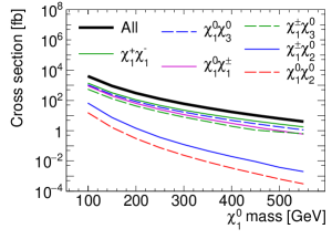
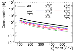
The production cross sections are shown in Figure 1.

(a) $\tan\beta$=1.

(b) $\tan\beta$=15.

Figure 1: Production cross sections in $pp$ collisions at $\sqrt{s}=8$ TeV at leading order for models of compressed spectra as a function of the mass of the lightest SUSY particle, $\chi_{1}^{0}$, for various combinations of gaugino modes. Other gaugino modes in which the cross sections are significantly smaller are not considered.

IV Analysis

Two ATLAS datasets are reinterpreted to constrain the models described above. The first is a broad ATLAS search for new phenomena in events with one or more jet and large missing transverse momentum (“mono-jet”) Aad et al. (2015a). The second is a search for vector-boson fusion (VBF) production of a Higgs boson which subsequenetly decays invisibly, giving two forward jets and large missing transverse momentum Aad et al. (2015b).

IV.1 Mono-jet Selection

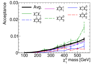
The mono-jet search Aad et al. (2015a) defines accepted jets as those with $p_{\rm T}>30$ GeV and $|\eta|<4.5$. The leading jet must satisfy $p_{\rm T}>120$ GeV and $|\eta|<2$. The ratio of the leading jet transverse momentum and the missing transverse momentum must be greater than 0.5. No jet may be within $\Delta\phi=1$ of the missing transverse momentum. There are nine signal regions characterized by their increasingly tighter requirements on the missing transverse momentum, $E_{\rm T}^{\rm miss}>$ 150, 200, 250, 300, 350, 400, 500, 600, 700 GeV. Events with leptons are vetoed.

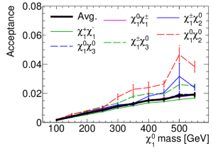
The acceptance, the fraction of events which survive this selection, is shown for each production case in Figure 2. The cross-section-weighted average is also shown.

(a) $\tan\beta$=1.

(b) $\tan\beta$=15.

Figure 2: Acceptance of the mono-jet selection for $E_{\rm T}^{\rm miss}>$ 400 GeV is measured with simulated events at $\sqrt{s}=8$ TeV at leading order for models of compressed spectra as a function of the mass of the lightest SUSY particle, $\chi_{1}^{0}$, for various combinations of gaugino modes. Also shown is the cross-section weighted average.

IV.2 VBF Selection

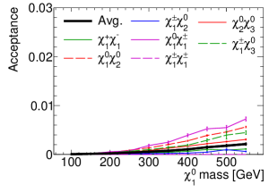
The VBF analysis Aad et al. (2015b) requires missing transverse momentum be greater than 150 GeV, the leading and sub-leading jet $p_{\rm T}$ be greater than 75 and 50 GeV, respectively. The product of the leading and sub-leading jets’ $\eta$ must be less than zero. The absolute value of the difference in the leading and sub-leading jets’ $\eta$ and $\phi$ must be greater than 4.8 and less than 2.5, respectively. The mass of the jet pair must be greater than 1 TeV. No jet may be within $\Delta\phi=1$ of the missing transverse momentum. Any events with more than 2 jets with $p_{\rm T}>30$ GeV and $|\eta|<4.5$ are vetoed. Events with leptons are vetoed.

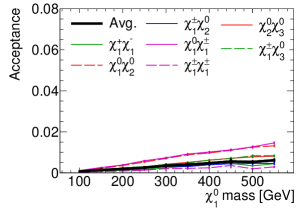
The acceptance, the fraction of events which survive this selection, is shown for each production case in Figure 3. The cross-section-weighted average is also shown.

(a) $\tan\beta$=1.

(b) $\tan\beta$=15.

Figure 3: Acceptance of the VBF selection measured with simulated events at $\sqrt{s}=8$ TeV at leading order for models of compressed spectra as a function of the mass of the lightest SUSY particle, $\chi_{1}^{0}$, for various combinations of gaugino modes. Also shown is the cross-section weighted average.

V Model reinterpretation

V.1 Procedure

In both the mono-jet and VBF cases, ATLAS provides model-independent upper limits on the visible production cross section:

$$\sigma_{\textrm{vis}}=\sigma\times\epsilon\times\cal{A}$$

where the acceptance $\cal{A}$ is the fraction of generated events which fall into the specified fiducial region and $\epsilon$ is the reconstruction efficiency inside the fiducial region. Typically the model dependence is captured by $\cal{A}$ and can be measured at the parton-level, while $\epsilon$ is fairly model-independent and reported by the experiment. Applying the dataset to our models therefore only requires measuring $\cal{A}_{\rm SUSY}$ so that one can calculate:

$$\sigma^{\rm limit}_{\rm SUSY}=\frac{\sigma_{\rm vis}}{\cal{A}_{\rm SUSY}\times\epsilon}.$$

V.2 Mono-jet Dataset

The mono-jet analysis reports limits for nine different signal regions defined by different $E^{\rm miss}_{\rm T}$ requirements; see Tab. 1. The reconstruction efficiency $\epsilon$ is reported for four different signal regions and ranges from 81% to 88%. We use a linear interpolation to calculate the efficiencies for the intermediate regions. We choose the signal region which gives the tightest expected limits in each case. See Tab. 3 for details.

Table 1: Observed and expected upper limits on $\sigma_{\textrm{vis}}$ at 95% CL from the ATLAS mono-jet dataset Aad et al. (2015a).

	Observed	Expected
$E^{\rm miss}_{\rm T}>$	limit [fb]	limit [fb]
$150$ GeV	726	935
$200$ GeV	194	271
$250$ GeV	90	106
$300$ GeV	45	51
$350$ GeV	21	29
$400$ GeV	12	17
$500$ GeV	7.2	7.2
$600$ GeV	3.8	3.6
$700$ GeV	3.4	1.8

V.3 VBF Dataset

An expected (observed) upper limit on $\sigma_{\textrm{vis}}$ at 95% confidence level is reported as 4.8 (3.9) fb from the VBF dataset. The reconstruction efficiency $\epsilon$ is 94% Aad et al. (2015b). Together with $\cal{A}_{\textrm{SUSY}}$ this allows calculation of upper limits on the SUSY models described above.

V.4 Results

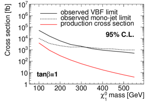
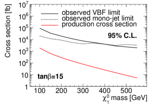
Upper limits on the pair-production of gauginos in association with jets from the mono-jet and VBF datasets are shown in Fig 4 and Table 3 along with the theoretical production cross-section at leading order.

Table 2: For $\tan\beta=$1, details of the theory production cross section $\sigma_{\textrm{Theory}}$, and for both the mono-jet and VBF datasets: the acceptance $\cal{A}$, reconstruction efficiency $\epsilon$, and 95% CL upper limit $\sigma^{\textrm{Limit}}$ for various choices of the $\chi_{1}^{0}$ mass. In the mono-jet case, the selected signal region (see Tab. 1) is also indicated.

$m_{\chi^{0}_{1}}$	$\sigma_{\textrm{Theory}}$	mono-jet				VBF
(GeV)	(fb)	SR${}_{\textrm{mono-jet}}$	$\cal{A}_{\textrm{mono-jet}}$	$\epsilon_{\textrm{mono-jet}}$	$\sigma^{\textrm{Limit}}_{\textrm{mono-jet}}$ (fb)	$\cal{A}_{\textrm{VBF}}$	$\epsilon_{\textrm{VBF}}$	$\sigma^{\textrm{Limit}}_{\textrm{VBF}}$ (fb)
100	4010	4	0.0053	0.83	10000	$8.2\times 10^{-5}$	0.94	51000
150	908	6	0.0040	0.83	3600	$2.6\times 10^{-4}$	0.94	16000
200	305	6	0.0064	0.83	2300	$6.8\times 10^{-4}$	0.94	6200
250	127	6	0.0085	0.83	1700	$1.4\times 10^{-3}$	0.94	2900
300	60.2	7	0.0048	0.82	1800	$2.1\times 10^{-3}$	0.94	2000
350	31.6	7	0.0056	0.82	1600	$3.3\times 10^{-3}$	0.94	1300
400	17.4	7	0.0069	0.82	1300	$4.3\times 10^{-3}$	0.94	970
450	10.3	7	0.0073	0.82	1200	$5.4\times 10^{-3}$	0.94	770
500	6.3	7	0.0089	0.82	990	$6.7\times 10^{-3}$	0.94	630
550	4.0	7	0.0090	0.82	970	$8.2\times 10^{-3}$	0.94	510

Table 3: For $\tan\beta$=15, details of the theory production cross section $\sigma_{\textrm{Theory}}$, and for both the mono-jet and VBF datasets: the acceptance $\cal{A}$, reconstruction efficiency $\epsilon$, and 95% CL upper limit $\sigma^{\textrm{Limit}}$ for various choices of the $\chi_{1}^{0}$ mass. In the mono-jet case, the selected signal region (see Tab. 1) is also indicated.

$m_{\chi^{0}_{1}}$	$\sigma_{\textrm{Theory}}$	mono-jet				VBF
(GeV)	(fb)	SR${}_{\textrm{mono-jet}}$	$\cal{A}_{\textrm{mono-jet}}$	$\epsilon_{\textrm{mono-jet}}$	$\sigma^{\textrm{Limit}}_{\textrm{mono-jet}}$ (fb)	$\cal{A}_{\textrm{VBF}}$	$\epsilon_{\textrm{VBF}}$	$\sigma^{\textrm{Limit}}_{\textrm{VBF}}$ (fb)
100	1890	3	0.0054	0.83	20000	$4.5\times 10^{-5}$	0.94	93000
150	630	3	0.0092	0.83	12000	$1.2\times 10^{-4}$	0.94	35000
200	286	4	0.0061	0.83	8900	$2.1\times 10^{-4}$	0.94	20000
250	144	5	0.0046	0.83	5600	$3.6\times 10^{-4}$	0.94	12000
300	78.8	6	0.0035	0.82	4200	$5.6\times 10^{-4}$	0.94	7500
350	44.4	7	0.0018	0.82	5000	$7.5\times 10^{-4}$	0.94	5600
400	25.5	7	0.0022	0.82	4000	$1.0\times 10^{-3}$	0.94	4000
450	14.9	7	0.0028	0.82	3100	$1.5\times 10^{-3}$	0.94	2800
500	8.8	7	0.0023	0.82	3800	$1.8\times 10^{-3}$	0.94	2300
550	5.3	7	0.0027	0.82	3300	$2.1\times 10^{-3}$	0.94	2000

(a) $\tan\beta$=1.

(b) $\tan\beta$=15.

Figure 4: Limits at 95% confidence level on the production cross section of compressed spectra models as a function of the mass of the lightest SUSY particle using the ATLAS VBF and mono-jet datasets.

VI Discussion

This is the first application of the VBF dataset to these SUSY scenarios. Neither dataset provides limits within an order of magnitude of the theoretical prediction, highlighting the challenge of probing these SUSY scenarios. However, we note that the mono-jet and VBF datasets have complementary sensitivity, as mono-jet dominates at lower $\chi_{0}$ mass and the VBF dataset is more powerful for more massive $\chi_{0}$. In the case of $\tan\beta=1$, the limits are within a factor of five of the theoretical prediction. Similar searches at $\sqrt{s}=13$ TeV will yield considerably more stringent limits.

References

- Csaki (1996) C. Csaki, Mod. Phys. Lett. A11, 599 (1996), arXiv:hep-ph/9606414 [hep-ph] .
- Rosiek (1990) J. Rosiek, Phys. Rev. D41, 3464 (1990).
- Arkani-Hamed et al. (2006) N. Arkani-Hamed, A. Delgado, and G. Giudice, Nucl.Phys. B741, 108 (2006), arXiv:hep-ph/0601041 [hep-ph] .
- Aad et al. (2015a) G. Aad et al. (ATLAS), Eur. Phys. J. C75, 299 (2015a), arXiv:1502.01518 [hep-ex] .
- Aad et al. (2015b) G. Aad et al. (ATLAS), (2015b), arXiv:1508.07869 [hep-ex] .
- Schwaller and Zurita (2014) P. Schwaller and J. Zurita, JHEP 03, 060 (2014), arXiv:1312.7350 [hep-ph] .
- Han et al. (2014) C. Han, A. Kobakhidze, N. Liu, A. Saavedra, L. Wu, and J. M. Yang, JHEP 02, 049 (2014), arXiv:1310.4274 [hep-ph] .
- Han et al. (2015) C. Han, L. Wu, J. M. Yang, M. Zhang, and Y. Zhang, Phys. Rev. D91, 055030 (2015), arXiv:1409.4533 [hep-ph] .
- Aad et al. (2015c) G. Aad et al. (ATLAS), (2015c), arXiv:1508.06608 [hep-ex] .
- Arbey et al. (2015) A. Arbey, M. Battaglia, and F. Mahmoudi, (2015), arXiv:1506.02148 [hep-ph] .
- Giudice et al. (2010) G. F. Giudice, T. Han, K. Wang, and L.-T. Wang, Phys.Rev. D81, 115011 (2010), arXiv:1004.4902 [hep-ph] .
- Dutta et al. (2013) B. Dutta, A. Gurrola, W. Johns, T. Kamon, P. Sheldon, and K. Sinha, Phys. Rev. D87, 035029 (2013), arXiv:1210.0964 [hep-ph] .
- Delannoy et al. (2013a) A. G. Delannoy, B. Dutta, A. Gurrola, W. Johns, T. Kamon, E. Luiggi, A. Melo, P. Sheldon, K. Sinha, K. Wang, and S. Wu, Phys. Rev. Lett. 111, 061801 (2013a), arXiv:1304.7779 [hep-ph] .
- Delannoy et al. (2013b) A. G. Delannoy, B. Dutta, A. Gurrola, W. Johns, T. Kamon, et al., (2013b), arXiv:1308.0355 [hep-ph] .
- Gelmini and Gondolo (2010) G. Gelmini and P. Gondolo, (2010), arXiv:1009.3690 [astro-ph.CO] .
- Cheung et al. (2013) C. Cheung, L. J. Hall, D. Pinner, and J. T. Ruderman, JHEP 05, 100 (2013), arXiv:1211.4873 [hep-ph] .
- Feng et al. (2000) J. L. Feng, K. T. Matchev, and F. Wilczek, Phys. Lett. B482, 388 (2000), arXiv:hep-ph/0004043 [hep-ph] .
- Feng et al. (2001) J. L. Feng, K. T. Matchev, and F. Wilczek, Phys. Rev. D63, 045024 (2001), arXiv:astro-ph/0008115 [astro-ph] .
- Baer et al. (2002) H. Baer, C. Balazs, and A. Belyaev, JHEP 03, 042 (2002), arXiv:hep-ph/0202076 [hep-ph] .
- Giudice and Romanino (2004) G. F. Giudice and A. Romanino, Nucl. Phys. B699, 65 (2004), [Erratum: Nucl. Phys.B706,65(2005)], arXiv:hep-ph/0406088 [hep-ph] .
- Pierce (2004) A. Pierce, Phys. Rev. D70, 075006 (2004), arXiv:hep-ph/0406144 [hep-ph] .
- Masiero et al. (2005) A. Masiero, S. Profumo, and P. Ullio, Nucl. Phys. B712, 86 (2005), arXiv:hep-ph/0412058 [hep-ph] .
- Baer et al. (2007) H. Baer, A. Mustafayev, E.-K. Park, and X. Tata, JCAP 0701, 017 (2007), arXiv:hep-ph/0611387 [hep-ph] .
- Griest and Seckel (1991) K. Griest and D. Seckel, Phys. Rev. D43, 3191 (1991).
- Gogoladze et al. (2011) I. Gogoladze, R. Khalid, Y. Mimura, and Q. Shafi, Phys. Rev. D83, 095007 (2011), arXiv:1012.1613 [hep-ph] .
- Djouadi et al. (2015) A. Djouadi, L. Maiani, A. Polosa, J. Quevillon, and V. Riquer, JHEP 06, 168 (2015), arXiv:1502.05653 [hep-ph] .
- Djouadi et al. (2013) A. Djouadi, L. Maiani, G. Moreau, A. Polosa, J. Quevillon, and V. Riquer, Eur. Phys. J. C73, 2650 (2013), arXiv:1307.5205 [hep-ph] .
- Djouadi and Quevillon (2013) A. Djouadi and J. Quevillon, JHEP 10, 028 (2013), arXiv:1304.1787 [hep-ph] .
- Bernal et al. (2007) N. Bernal, A. Djouadi, and P. Slavich, JHEP 07, 016 (2007), arXiv:0705.1496 [hep-ph] .
- Cahill-Rowley et al. (2015) M. Cahill-Rowley, J. L. Hewett, A. Ismail, and T. G. Rizzo, Phys. Rev. D91, 055002 (2015), arXiv:1407.4130 [hep-ph] .
- Cohen et al. (2012) T. Cohen, J. Kearney, A. Pierce, and D. Tucker-Smith, Phys. Rev. D85, 075003 (2012), arXiv:1109.2604 [hep-ph] .
- Alwall et al. (2011) J. Alwall, M. Herquet, F. Maltoni, O. Mattelaer, and T. Stelzer, JHEP 1106, 128 (2011), arXiv:1106.0522 [hep-ph] .
- Sjostrand et al. (2006) T. Sjostrand, S. Mrenna, and P. Z. Skands, JHEP 0605, 026 (2006), arXiv:hep-ph/0603175 [hep-ph] .